Equilibria, periodic orbits and computing them.
EPSRC Summer School on Modal decompositions in fluid mechanics.
DAMTP, Cambridge, 5-8 August 2019.
Ashley P. Willis,
School of Mathematics and Statistics,
University of Sheffield, U.K.
a.p.willis@sheffield.ac.uk, openpipeflow.org.
In this short exposition, we describe equilibria and periodic orbits in terms of the flow map, , and discuss the essentials of the Jacobian-free Newton–Krylov (JFNK) method that can be used to find them. This method requires little more than calls to an existing time stepping code, which can be considered to represent. Fortran90 / MATLAB code is available to try it out for yourself, where, in the template/example the method is applied to the Lorenz system. This code is problem-independent and can be applied to large systems, having initially been developed to find periodic orbits in simulations of pipe flow.
1 Using the flow-map
Let the point be an -vector representing the state of a system. For a dynamical system, as time progresses, the point traces out a trajectory, a one-dimensional curve, in an -dimensional phase space .
We can describe the trajectory for using the flow-map denoted , which takes a point and evolves it by a time period : i.e.
| (1.1) |
More generally, the flow-map simply advances a point along its trajectory:
| (1.2) |
1.1 Example: Lorenz’s model for convection
Lorenz 1963 derived the following system for three-time dependent amplitudes, , and :
| (1.3) | |||||
At each instant in time, the current state is a point in the phase space . As time progresses, traces out a trajectory, i.e. a curve, in . Lorenz focussed on parameter values , , , which result in chaotic trajectories. The flow-map takes us along this trajectory, see figure 1.
(a)
 (b)
(b)
We should not forget that each point in phase-space corresponds to a whole convection flow pattern! Here it corresponds to a two-dimensional flow between two flat plates a distance apart, with a temperature difference between the top and bottom plates (figure 2).
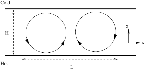
The amplitudes , , correspond to modulated variations in the temperature and velocity fields:
where the are scalar constants.
1.2 Invariant solutions
Equilibria and periodic orbits are topological features of the phase space . Irrespective of the coordinates and measure of distance used to visualise the phase space, an equilibrium remains a point, and a periodic orbit remains a closed loop. Properties, such as their eigenvalues, are also invariant to the measure of distance used.
An equilibrium is a fixed point of the flow-map that satisfies
| (1.4) |
for any time . A point on a periodic orbit satisfies
| (1.5) |
where is the period of the orbit. In terms of solutions of the flow-map, we can consider an equilibrium to be a special case of a periodic orbit where may be arbitrarily chosen.
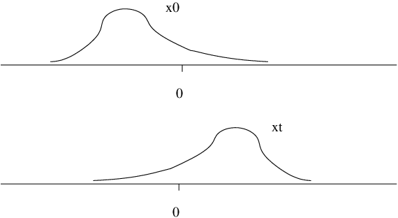
If a system has a homogeneous dimension, , then it can have travelling wave solutions. (See figure 3a.) In a frame moving at some phase speed , the solution looks steady. Equivalently, we can keep shifting the solution so that it looks steady. Let be an operator that shifts a state by a distance in the direction. Then, a travelling wave satisfies
| (1.6) |
for any time . The state is an equilibrium solution of the slightly modified map for any , hence we also call a travelling wave a relative equilibrium. Similarly, a periodic solution that recurs up to a spatial shift,
| (1.7) |
for some , we call a relative periodic orbit.
Suppose the dimension has a mirror symmetry about . Let be the flip operator: . The second half of an orbit satisfying (1.5) might just be a reflection of the first half:
| (1.8) |
(See figure 3b.) Such orbits are called pre-periodic orbits. The shortest/simplest periodic orbits of a system with discrete symmetries are typically pre-periodic. Figure 4 shows the shortest periodic orbit of the Lorenz system, where the second half of the orbit is related to the first half by the 180 degree rotation symmetry .
(a)
 (b)
(b)

1.3 Poincaré sections
Let be a point and be a normal vector that together define a hypersurface . Crossings of can be defined by times when . (See figure 5a.) We might restrict to when crossings occur in a particular direction, say when the inner product goes from negative to positive.
We can now let be the map that takes one point on to the next crossing point on . If a periodic orbit has a point on , then it satisfies
| (1.9) |
The advantage is that we no longer need to worry about the period for periodic orbits. The disadvantage is that we know nothing about what happens to the orbit off , and in general, not all periodic orbits cross a single .
(a) (b)
(b)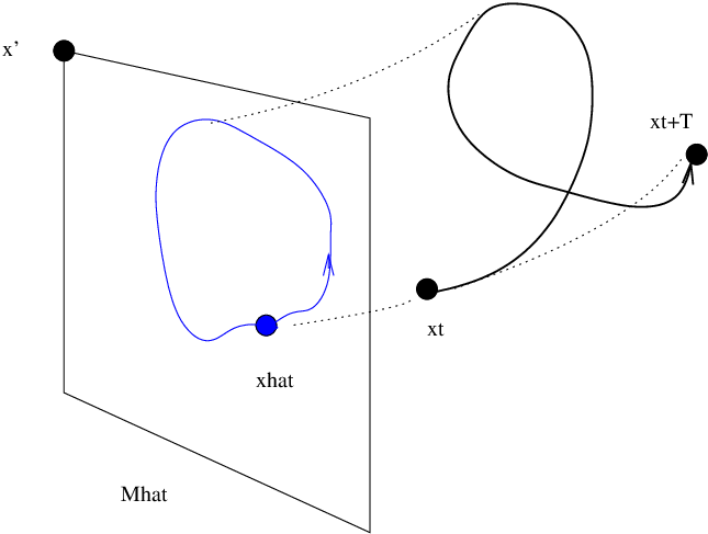
1.4 Slicing
For a homogeneous spatial dimension , the freedom of a pattern to appear at any location is awkward when we want to compare states. Slicing is an automatic shifting procedure that removes this degree of freedom.
Here we will discuss the simplest form of slicing – ‘Fourier’ slicing. (Budanur et al. 2015; Willis et al. 2016, See) When a system has a homogeneous dimension, it is commonplace to work with a periodic domain of length . In this case, construct where and are arbitrary states independent of ; they must not both be zero.
Any state may be projected onto a plane via and . (See figure 6a.) In this projection, the set of shifted states lie on a circle centred on the origin. By shifting the states, we can rotate all points on the circle to the unique point on the circle where it crosses the positive axis. All possible shifted versions of are then mapped to the unique version , where and is the polar angle to .
This operation is a symmetry-reduction, and we say that the symmetry-reduced state , indicated by the hat, lies on a slice. Arbitrary shifts have been eliminated, so the slice has dimension one less than that of the original system. The slice is a hypersurface within the original space of states .
The slice is different from a Poincaré section because the symmetry reduction can be applied to for all times . We can compute sliced dynamics with trajectories that lie within the slice. (See figure 5b.) Meanwhile, trajectories only pierce a Poincaré section.
Relative equilibria (travelling waves) are reduced to equilibria automatically:
| (1.10) |
All possible shifts of a state are reduced by shifting to one particular version on the slice , i.e. the travelling wave is ‘pinned’ by the shifting. (See figure 6b.) Here, is the flow-map of the symmetry reduced dynamics. Note that all travelling waves of the system are reduced to equilibria, even though they typically will have a range of different phase speeds .
Similarly, a relative periodic orbit becomes a closed periodic orbit, because the start and end point are shifted to a single point on . The relative periodic orbit now satisfies the simpler form:
| (1.11) |
for any symmetry-reduced point on the orbit.
(a)
 (b)
(b)

2 Periodic orbits
All periodic orbits (POs) in a chaotic attractor must be unstable, otherwise the behaviour would eventually be attracted to the orbit and become periodic, not chaotic. So why is it useful to find POs when they’re all unstable!?
2.1 Why periodic orbits?
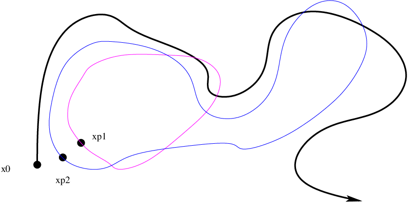
Firstly, the dynamics is always very close to a PO! A chaotic attractor is dense in POs: For any chaotic point and , there exists a periodic point within of . See figure 7. Also…
- •
Unlike equilibria, POs exhibit dynamics! — they capture the time-dependent dynamic processes of the system and organise the chaotic set.
- •
The chaotic dynamics tends to follow the least unstable POs.
- •
A PO is a closed loop in state space. It will appear as a closed loop irrespective of the coordinates used to visualise the state space.
- •
The shortest, most fundamental, POs provide an alphabet for symbolic dynamics.
- •
Statistical properties of a chaotic attractor can be calculated in terms of sums over the POs, using their relative stability.
2.2 Examples of periodic orbits
- •
The logistic map is chaotic for the case but has the (unstable) period- orbit
- •
In a remarkable methodical and computational feat, Viswanath 2003 calculated 111011 periodic orbits of the Lorenz attractor, that is all periodic orbits with itineraries of up to length 20 (number of windings around the left/right ‘wings’), with an accuracy of 14 decimal digits. A few of them are shown in figure 8. The periodic orbit was found to be the least unstable among all orbits calculated. (It is the periodic orbit with the smallest Lyapunov/Floquet exponent.)


Figure 8: A few of the shortest periodic orbits of the Lorenz system. (Viswanath 2003, Reproduction of figure 3 of) - •
For an 154755-dimensional model of turbulent flow in a pipe, Willis et al. 2016 calculated periodic orbits and travelling wave solutions. Travelling waves are stationary in a moving frame, so they correspond to fixed points in the sliced phase space. Two ‘clouds’ of solutions were observed, shown in figure 9, and the relationship between them found to be the reflection symmetry. The phase-space visualisation reveals that trajectories don’t like to switch orientation with respect to the symmetry, due to the presence of a strongly repelling (unstable) fixed point, marked ‘A’, that lives between the two clouds. For beautiful examples from Couette flow, see Cvitanović and Gibson 2010.


Figure 9: (left) Visualisation of pipe flow with slow streaks (blue) and vortices (yellow). (right) Periodic orbits of pipe flow. Inset is view from bottom left side of box. (Willis et al. 2016, Reproduction of figure 4 of)
2.3 Searching for recurrences
At present, the standard approach to finding near-recurrences is pretty crude. It involves recurrence plots, with distance measures tailored for the case at hand, and, if not automated, visual inspection of the plot for close recurrences. Nevertheless, this is the usual means to find points close to periodic orbits that can be refined to exact recurrences using the Newton method (described in the next section).

We then look for local minima in the plot that provide candidate recurrent points, and . The normalisation factor might be chosen to depend on both and , or might not be necessary at all. A complication is that we might need to minimise over discrete symmetries, such as the flip operator , or over shifts (section 1.2) e.g.
| (2.2) |
Minimisation over shifts can be avoided if slicing is applied (section 1.4).
The norm itself might need tinkering with. For example, in the sheared flow of fluid, perturbations in the streamwise dimension are typically an order of magnitude larger than the crossflow components. A ‘compensatory’ norm helps in this case, where the components are scaled to be more similar in magnitude.
3 The Newton–Krylov method
The Jacobian-free Newton–Krylov (JFNK) method is a variant of the Newton–Raphson method. In its raw form, the Newton–Raphson method for an -dimensional system involves an Jacobian matrix, which can be tricky to evaluate. It is possible to avoid this evaluation using a Krylov-subspace method (Knoll and Keyes 2004).
3.1 The Newton–Raphson method
To find roots such that in one dimension, given an initial guess , the Newton-Raphson method generates improvements using the iteration
| (3.1) |
Re-arranging, we may re-express the iteration as
| (3.2) |
Our task is to find fixed points of the map such that , i.e.
| (3.3) |
(The fixed points could correspond to equilibria, periodic orbits, or their relative equivalents. Augmentations, if necessary, to find a period or spatial shift are delayed to section 3.4.) The extension of Newton’s method (3.2) to an -dimensional system is then
| (3.4) |
In order to apply the update (3.4a), the linear system (3.4b) needs to be solved for the unknown .
In (3.4b), the matrix part is given by
| (3.5) |
where is the Jacobian matrix for and is the identity matrix. For the case ,
| (3.6) |
3.2 Jacobian-Free method
The Jacobian matrix is usually difficult to evaluate. We might not even have sufficient computer memory to store it for a high dimensional system. The problem (3.4b), however, is in the form
| (3.7) |
where is an matrix and and are -vectors. This can be solved for using the Krylov-subspace method GMRES(m). The GMRES algorithm does not need to know the matrix itself, only the result of multiplying a given vector by . The method seeks a solution for in , i.e. . It is common to start with . The next vector is generated by evaluating , then is obtained by orthonormalising against the previous () using the Gram-Schmidt method. Next, is minimised over the coefficients () and the process repeated if is too large.
Iterations of the GMRES algorithm for the problem (3.4b) involve calculating matrix-vector products with given that may be approximated:
| (3.8) |
is a small scalar value; a typical value is such that . The important point is that we do not need to know the Jacobian — only a routine for evaluating is required.
Note that provided that each step of the Newton method, , takes in approximately the correct direction, the method is expected to converge. Therefore the tolerance specified in the accuracy of the solution for in each Newton step (calculated via the GMRES method) typically need not be so stringent as the tolerance placed on the Newton method itself for the solution . For example, we might seek a relative error for the Newton solution , but a relative error for the GMRES solution is likely to be sufficient for calculation of the steps .
3.3 Hookstep approach
To improve the domain of convergence of the Newton method, it is commonplace to limit the size of the step taken. One approach is simply to take a ‘damped’ step in the direction of the solution to 3.4(b), i.e. step by , where . In the ”’hookstep approach”’, we minimise subject to the condition that the magnitude of the Newton step is limited, , where is the size of the ”’trust region”’:
| (3.9) |
Given the minimisation, the hookstep is expected to produce a better result than a simple damped step of the same size. It is also expected to perform much better in ’valleys’, where it produces a bent/hooked step to a point along the valley, rather than jumping from one side of the valley to the other; see figure 11.
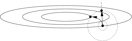
The hookstep can be calculated with little extra work to the GMRES method, provided that the size of Krylov-subspace, m, is chosen sufficiently large to solve to the desired accuracy within m GMRES iterations; for details see Viswanath 2007 [particularly v1 on arxiv.org].
For a given , the reduction in error predicted by the linearisation (3.9) can be compared with the actual reduction in . According to the accuracy of the prediction, the size of the trust region can be adjusted automatically; see Dennis and Schnabel 1996.
3.4 Adding constraints
3.4.1 Time constraint
When looking for a periodic orbit, the period is an extra unknown. One way to eliminate needing to find is to work within a Poincaré section, as described in section 1.3. We can then attempt to solve the function as it stands to find a point on the Poincaré section that corresponds to a periodic orbit.
We might not want to restrict ourselves to Poincaré sections. We must then solve
| (3.10) |
for . We augment the whole system. Let
| (3.11) |
We now want to solve a system of the form
| (3.12) |
for , but need an extra constraint because we have an extra unknown. We choose that the update has no component that points along the trajectory, i.e. . Following the ethos of matrix-free methods, that we do not need to know the matrix itself, we only need to state the result of multiplication by :
| (3.13) |
We use the approximation (3.8) to evaluate the first part of the result. The augmented system (3.12) can be solved for using the GMRES algorithm by applying multiplications (3.13). The update for both the state and the period is then .
3.4.2 Shift constraints
For relative equilibria (travelling waves) and relative periodic periodic orbits we need to solve
| (3.14) |
where is an unknown spatial shift in the homogeneous -dimension.
One way to avoid the extra unknown is to work with the sliced dynamics (section 1.4) so that arbitrary shifts are automatically eliminated. Alternatively, we can augment the system again. Let
| (3.15) |
We now want to solve a system of the form
| (3.16) |
for , but need another constraint to match the extra unknown. This time we choose that the update has no component that just corresponds to a spatial shift, i.e. . We assert that multiplication by is:
| (3.17) |
3.5 Preconditioning
The good news is that you can ignore preconditioning and skip this section if you are combining Newton–Krylov with timestepping to evaluate the flow-map .
3.5.1 Exponentiation and timestepping
The GMRES algorithm is closely related to another Krylov-subspace method, the Arnoldi method, which is used to calculated eigenvalues of a matrix . It tends to find the eigenvalues most separated in the complex plane first, but those might be of little interest. For example, the Laplacian has a spectrum of very negative eigenvalues corresponding to high frequency oscillations that rapidly decay. Basically, we do not wish to build a Kyrlov-subspace involving such modes.
It may be better to work with , corresponding to the eigenproblem . This problem shares the same eigenvectors as the problem , but has more suitable eigenvalues, . The negative eigenvalues then correspond to eigenvalues bunched close to the origin. The Arnoldi method then favours the most distant from the origin, corresponding to the with largest real parts.
Note that for the system , time integration corresponds to exponentiation: Taking eigenvector with growth rate as an initial condition, the result of time integration from to is . We therefore have that , which can be written where is the eigenvalue of the time integration operator .
3.5.2 Explicit preconditioning
GMRES is likely to find it easier to solve than the original system, if is an approximate inverse for . For example, if is dominated by its diagonal elements, we might take to be the banded matrix consisting of the diagonal and the first sub- and super-diagonals of . Each GMRES iteration applied to the modified system now requires a muliplication by then by . This is fine, as, for a banded matrix, it is quick and easy to solve for . Like , we don’t need to know the matrix itself, only the result of multiplication by the matrix.
4 Try it yourself! Application of the Newton–Krylov method to the Lorenz system
Given that the Newton–Krylov method is designed to cope with
high-dimensional systems (the same code has been used to find
travelling waves in pipe flow), this is somewhat overkill,
but it helps illustrates how we can use the solver as a
black box…
Please cite openpipeflow.org (Willis 2017) if you use this
code in your research. Thanks!
- •
Download the Template/Example (Fortran90 / MATLAB / Octave)
http://www.openpipeflow.org/index.php?title=Newton-Krylov_method - •
For MATLAB, the unpacked tgz/zip file has separate .m files for each function.
Take a look at- –
Lorenz_f.m: Lorenz evolution rule .
- –
steporbit.m: Evaluate , i.e. step by ndts_ timesteps, where the input x(1), and x(2:4). The timestep size is dtndts_.
- –
saveorbit.m: Output at end of each Newton iteration. relative_err.
- –
MAIN.m: Set up initial guess and call the black box NewtonHook.m.
- –
- •
Other functions are called by NewtonHook.m, and are unlikely to need changing for a problem of this type, where shifts and other spatial symmetries are ignored:
- –
getrhs.m: Evaluate right-hand side (3.11) i.e. .
- –
multJ.m : Evaluate multiplication (3.13), i.e. multiplication by the Jacobian.
- –
multJp.m: Preconditioner for multiplication (here an empty function).
- –
dotprd.m: Evaluate inner product .
- –
GMRESm.m: Method of section 3.2.
- –
GMREShook.m: Calculate hookstep, section 3.3.
- –
- •
The following data are points on the periodic orbits of figure 8, taken from Viswanath 2003. in call cases.
AB −13.763610682134 −19.578751942452 1.5586522107162 AAB −12.595115397689 −16.970525307084 2.3059072639399 AAAB −11.998523280062 −15.684254096883 3.0235837034339 AABB −12.915137970311 −17.673100172646 3.0842767758221 () - •
In MATLAB, call MAIN. It will plot the result of timestepping the initial guess for the AB orbit (green), call the NewtonHook subroutine, then plot the converged solution (blue). Scroll back through the output, and compare relative_err for the initial guess at iteration 0 with the final relative error.
- •
Comment/uncomment other initial guesses new_x, or experiment with your own. How do they affect the number of Newton iterations taken?
[Typically convergence takes iterations, otherwise it will never converge.] - •
Uncomment the initial guess for an equilibrium. Here we assume a short fixed , too short for a PO; is not permitted to change, otherwise could be reduced by simply taking . Check that MAIN can find the analytic equilibrium solution , where .
4.1 Adapting the code for your own use
- •
For a very large system, for which you might consider parallelization (see final comment), you should probably use the Fortran90 version.
- •
Experiment with the Template/Example first, to get used to how the code is set up. The initial guess is put in new_x.
- •
Note that at present, new_x(1) (the period), and new_x(2:end) (the state).
- •
The place to start is then steporbit. If you already have an existing timestepping code, it could do something as simple as call it externally via system calls:
function y = steporbit(ndts_,x) persistent dt if ndts_ ~= 1 % Set timestep size dt=T/ndts_ dt = x(1) / ndts_ ; % If only doing one step to calc \dot{x}, end % then use previously set dt. a = x(2:end) ; WRITE DATA TO FILES: dt timestep size ndts_ number of steps to take a initial condition LOAD STATE, TIMESTEP, SAVE STATE: system(’run_my_code.exe’) LOAD TIMESTEPPED STATE: --> a y = zeros(size(x)) ; y(2:end) = a ; end - •
saveorbit is called at the end of each Newton iteration. Add code here to save the current state new_x.
- •
If your inner product corresponds to where is a diagonal matrix of positive weights, and here is the transpose, then pass to the code. The existing functions that take inner products then need no modification.
- •
For parallel use with MPI+Fortran, the NewtonHook and GMRES codes do not need changing: Split vectors over threads and let each thread pass its section to NewtonHook. The only place where an MPI call is required is an MPI_Allreduce in the dotprod function. To avoid all threads outputting information, set info=1 on rank 0, and info=0 on all other ranks.
- •
Further information at openpipeflow.org.
Acknowledgements
AW would like to thank Rich Kerswell, Predrag Cvitanović (chaosbook.org), John Gibson (channelflow.org), Marc Avila and many others for their generous support in many forms. Developed under EPSRC grants EP/K03636X/1, EP/P000959/1.
References
- Budanur et al. (2015) Budanur, N. B., P. Cvitanović, R. L. Davidchack, and E. Siminos (2015). Reduction of the SO(2) symmetry for spatially extended dynamical systems. Phys. Rev. Lett. 114, 084102.
- Cvitanović and Gibson (2010) Cvitanović, P. and J. F. Gibson (2010). Geometry of turbulence in wall-bounded shear flows: Periodic orbits. Phys. Scr. T 142, 014007.
- Dennis and Schnabel (1996) Dennis, J. and R. Schnabel (1996). Numerical Methods for Unconstrained Optimization and Nonlinear Equations. SIAM.
- Knoll and Keyes (2004) Knoll, D. A. and D. E. Keyes (2004). Jacobian-free Newton–Krylov methods: a survey of approaches and applications. Journal of Computational Physics 193(2), 357–397.
- Lorenz (1963) Lorenz, E. N. (1963). Deterministic nonperiodic flow. J. Atmos. Sci. 20, 130–141.
- Viswanath (2003) Viswanath, D. (2003). Symbolic dynamics and periodic orbits of the Lorenz attractor. Nonlinearity 16, 1035–1056.
- Viswanath (2007) Viswanath, D. (2007). Recurrent motions within plane Couette turbulence. J. Fluid Mech. 580, 339–358.
- Willis (2017) Willis, A. (2017). The Openpipeflow Navier–Stokes solver. SoftwareX 6, 124–127.
- Willis et al. (2013) Willis, A. P., P. Cvitanović, and M. Avila (2013). Revealing the state space of turbulent pipe flow by symmetry reduction. J. Fluid Mech. 721, 514–540.
- Willis et al. (2016) Willis, A. P., K. Y. Short, and P. Cvitanović (2016). Symmetry reduction in high dimensions, illustrated in a turbulent pipe. Phys. Rev. E 93, 022204.