跳到论文正文
W Papers独立论文阅读器 arXiv:1908.06634 论文正文 计算阅读时间 · 0%
引用这篇论文根据当前论文元数据生成,正式投稿前建议核对。


License: arXiv.org perpetual non-exclusive license
arXiv:1908.06634v4 [cs.MA] 02 Apr 2021

Cluster-based Distributed Augmented Lagrangian Algorithm for a Class of Constrained Convex Optimization Problems footnoteinfo

Hossein Moradian Email: hmoradia@uci.edu    Solmaz S. Kia Email: solmaz@uci.edu
Abstract

We propose a distributed solution for a constrained convex optimization problem over a network of clustered agents each consisted of a set of subagents. The communication range of the clustered agents is such that they can form a connected undirected graph topology. The total cost in this optimization problem is the sum of the local convex costs of the subagents of each cluster. We seek a minimizer of this cost subject to a set of affine equality constraints, and a set of affine inequality constraints specifying the bounds on the decision variables if such bounds exist. We design our distributed algorithm in a cluster-based framework which results in a significant reduction in communication and computation costs. Our proposed distributed solution is a novel continuous-time algorithm that is linked to the augmented Lagrangian approach. It converges asymptotically when the local cost functions are convex and exponentially when they are strongly convex and have Lipschitz gradients. Moreover, we use an ϵ\epsilon-exact penalty function to address the inequality constraints and derive an explicit lower bound on the penalty function weight to guarantee convergence to ϵ\epsilon-neighborhood of the global minimum value of the cost. A numerical example demonstrates our results.

keywords
distributed constrained convex optimization, augmented Lagrangian, primal-dual solutions, optimal resource allocation, penalty function methods
††thanks: [††thanks: [††address: Department of Mechanical and Aerospace Engineering, University of California, Irvine

footnoteinfo]Corresponding author: H. Moradian  footnoteinfo]This work was supported by NSF, United States of America, CAREER award ECCS-1653838. A preliminary version of this paper is presented in [1].

1 Introduction

We consider a group of NN clustered agents 𝒱={1,⋯,N}\mathcal{V}=\{1,\cdots,N\} with communication and computation capabilities, whose communication range is such that they can form a connected undirected graph topology, see Fig. 1. These agents aim to solve, in a distributed manner, the optimization problem

𝘅⋆\displaystyle\boldsymbol{\mathbf{\mathsf{x}}}^{\star} =argmin𝐱∈m∑i=1Nfi(𝐱i),subject to\displaystyle=\arg\min_{\boldsymbol{\mathbf{x}}\in\real^{m}}\,\,\sum\nolimits_{i=1}^{N}f^{i}(\boldsymbol{\mathbf{x}}^{i}),~~\text{subject~to~} (1a)
[𝘄1]j​𝐱1+⋯+[𝘄N]j​𝐱N−𝖻j=0,j∈{1,⋯,p},\displaystyle\!\!\!\!\!\!\![\boldsymbol{\mathbf{\mathsf{w}}}^{1}]_{j}\boldsymbol{\mathbf{x}}^{1}\!\!+\cdots+[\boldsymbol{\mathbf{\mathsf{w}}}^{N}]_{j}\boldsymbol{\mathbf{x}}^{N}\!\!-\mathsf{b}_{j}\!=\!0,\,\,j\in\{1,\cdots,p\}, (1b)
𝗑¯li≤xli,l∈ℬ¯i⊆{1,⋯,ni},i∈𝒱,\displaystyle\underline{\mathsf{x}\mkern-2.0mu}\mkern 2.0mu^{i}_{l}\leq{x}^{i}_{l},\quad\,\,\,l\in\underline{\mathcal{B}}^{i}\subseteq\{1,\cdots,n^{i}\},\quad i\in\mathcal{V}, (1c)
xli≤𝗑¯li,l∈ℬ¯i⊆{1,⋯,ni},i∈𝒱,\displaystyle{x}^{i}_{l}\leq\bar{\mathsf{x}}^{i}_{l},\quad\,\,\,l\in\bar{\mathcal{B}}^{i}\subseteq\{1,\cdots,n^{i}\},\quad i\in\mathcal{V}, (1d)

where fi​(𝐱i)=∑l=1nifli​(xli).f^{i}(\boldsymbol{\mathbf{x}}^{i})=\sum\nolimits_{l=1}^{n^{i}}f_{l}^{i}(x_{l}^{i}). In this setting, each agent i∈𝒱i\in\mathcal{V} is a cluster of local ‘subagents’ l∈{1,…,ni}l\in\{1,\dots,n^{i}\} whose decision variable is 𝐱i=[x1i,⋯,xnii]⊤∈ni\boldsymbol{\mathbf{x}}^{i}=[x^{i}_{1},\cdots,{x}^{i}_{n^{i}}]^{\top}\in\real^{n^{i}}. The weighting factor matrix 𝘄i∈p×ni\boldsymbol{\mathbf{\mathsf{w}}}^{i}\in\real^{p\times n^{i}} of each agent i∈𝒱i\in\mathcal{V} is only known to the agent ii itself. Moreover, 𝗑¯li,𝗑¯li∈\underline{\mathsf{x}\mkern-2.0mu}\mkern 2.0mu^{i}_{l},\bar{\mathsf{x}}^{i}_{l}\in\real, with 𝗑¯li<𝗑¯li\underline{\mathsf{x}\mkern-2.0mu}\mkern 2.0mu^{i}_{l}<\bar{\mathsf{x}}^{i}_{l}, are respectively the lower and upper bounds on the lthl^{\text{th}} decision variable of agent i∈𝒱i\in\mathcal{V}, if such a bound exists. In a distributed solution, each agent i∈𝒱i\in\mathcal{V} should obtain its respective component of 𝘅⋆=[𝘅1⋆⊤,⋯,𝘅N⋆⊤]⊤\boldsymbol{\mathbf{\mathsf{x}}}^{\star}=[{\boldsymbol{\mathbf{\mathsf{x}}}^{1\star\top}},\cdots,{\boldsymbol{\mathbf{\mathsf{x}}}^{N\star\top}}]^{\top} by interacting only with the agents that are in its communication range. Problem (1) explicitly or implicitly, captures various in-network optimization problems. One example is the optimal in-network resource allocation, which appears in many optimal decision making tasks such as economic dispatch over power networks [2, 3], optimal routing [4, 5] and network resource allocation for wireless systems [6, 7]. In such problems, a group of agents with limited resources, e.g., a group of generators in a power network, add up their local resources to meet a demand in a way that the overall cost is optimum for the entire network. Another family of problems that can be modeled as (1) is the in-network model predictive control over a finite horizon for a group of agents with linear dynamics [8, 9].

In recent years, there has been a surge in the design of distributed algorithms for large-scale in-network optimization problems. The major developments have been in the unconstrained convex optimization setting where the global cost is the sum of local costs of the agents (see e.g. [10, 11]for algorithms in discrete-time, and [12, 13, 14] for algorithms in continuous-time). In-network constrained convex optimization problems have also been studied in the literature. For example, in the context of the power generator economic dispatch problem, [15, 16, 17] offer distributed solutions that solve a special case of (1) with local quadratic costs subject to bounded decision variables and a single demand equation, p=1p=1 and 𝗐i=1\mathsf{w}^{i}=1 for i∈𝒱i\in\mathcal{V}. Distributed algorithm design for special cases of (1) with non-quadratic costs are presented in [18, 19, 8] in discrete-time form, and [20, 21, 22, 23, 24] in continuous-time form. Except for [19], all these algorithms consider the case that the local decision variable of each agent i∈𝒱i\in\mathcal{V} is a scalar. Moreover, with the exception of [21, 19, 8], these algorithms only solve (1) when the equality constraint is the unweighted sum of local decision variables, i.e., p=1p=1 and 𝗐i=1\mathsf{w}^{i}=1 for i∈𝒱i\in\mathcal{V}. Also, only  [23] and [24] consider local inequality constraints, which are in the form of local box inequality constraints on all the decision variables of the problem. Lastly, the algorithms in [18, 23, 24] require the agents to communicate the gradient of their local cost functions to their neighbors. Such a requirement can be of concern for privacy-sensitive applications.

Refer to caption
Figure 1: A group of clustered agents (generators) with undirected connected graph topology aim to solve 𝘅⋆=arg⁡min⁡∑i=16𝐱∈ℝ12⁡fi​(𝐱i)\boldsymbol{\mathbf{\mathsf{x}}}^{\star}=\arg\min_{\boldsymbol{\mathbf{x}}\in{\mathbb{R}}^{12}}\sum\nolimits_{i=1}^{6}f^{i}(\boldsymbol{\mathbf{x}}^{i}), subject to [1​1]​𝐱1+𝐱2+[0.5​0.5​0.5]​𝐱3+[1  1  1]​𝐱4=450[1~1]\boldsymbol{\mathbf{x}}^{1}+\,\boldsymbol{\mathbf{x}}^{2}+[0.5~0.5~0.5]\boldsymbol{\mathbf{x}}^{3}+\,[1\,\,1\,\,1]\boldsymbol{\mathbf{x}}^{4}=450, [0.5​0.5​0.5]​𝐱3+[1​1]​𝐱5+𝐱6=700[0.5~0.5~0.5]\boldsymbol{\mathbf{x}}^{3}+[1~1]\,\boldsymbol{\mathbf{x}}^{5}+\boldsymbol{\mathbf{x}}^{6}=700, and 𝗑¯li≤xli≤𝗑¯li,i∈ℤ16,l∈ℤ1ni\underline{\mathsf{x}\mkern-2.0mu}\mkern 2.0mu^{i}_{l}\!\leq\!x^{i}_{l}\!\leq\!\bar{\mathsf{x}}^{i}_{l},\hskip 8.19447pt\hskip 8.19447pti\!\in\!\mathbb{Z}_{1}^{6},\hskip 8.19447ptl\!\in\!\mathbb{Z}_{1}^{n^{i}} in a distributed manner. Here, fi​(𝐱i)=∑l=1nifli​(xli)f^{i}(\boldsymbol{\mathbf{x}}^{i})=\sum_{l=1}^{n^{i}}f^{i}_{l}(x^{i}_{l}), where fli(xli)=αlixli+2βlixli+γlif^{i}_{l}(x^{i}_{l})=\alpha^{i}_{l}x^{i}_{l}\,\!{}^{2}+\beta^{i}_{l}x^{i}_{l}+\gamma^{i}_{l}. In the physical layer plot, a cluster agent can communicate with another cluster if it is inside the other cluster’s communication disk. To solve this optimal resource allocation problem in a distributed manner, we form subgraphs 𝒢1​(𝒱1,ℰ1)\mathcal{G}_{1}(\mathcal{V}_{1},\mathcal{E}_{1}) and 𝒢2​(𝒱2,ℰ2)\mathcal{G}_{2}(\mathcal{V}_{2},\mathcal{E}_{2}), which are associated, respectively, with the first and the second equality constraints. Here, 𝒱1={1,2,3,4}\mathcal{V}_{1}=\{1,2,3,4\} and 𝒱2={3,4,5,6}\mathcal{V}_{2}=\{3,4,5,6\}. Agent 44 acts as a connectivity helper node in 𝒢2\mathcal{G}_{2}. A solution to this problem using our proposed algorithm is given in section 4.

In this paper, we propose a novel distributed algorithm to solve the optimization problem (1). We start by considering the case that ℬ¯i=ℬ¯i={}\underline{\mathcal{B}}^{i}=\bar{\mathcal{B}}^{i}=\{\} for i∈𝒱i\in\mathcal{V}, i.e., when there is no inequality constraint. For this problem, we propose a continuous-time distributed primal-dual algorithm. To induce robustness and also to yield convergence without strict convexity of the local cost functions, we adapt an augmented Lagrangian framework [25]. The augmented Lagrangian method has been used in [26], [27], and [19] to improve the transient response of the distributed algorithms for, respectively, an unconstrained convex optimization, an online optimization, and a discrete-time constrained optimization problems. Different than the customary practice of using a common augmented Lagrangian penalty parameter as in [19, 27, 26], in our design to reduce the coordination overhead among the agents we allow each agent to choose its own penalty parameter locally. The structure of our distributed solution is inspired by the primal-dual centralized solution of [28] (see (6)), where the coupling in the differential solver is in the dual state dynamics. In decentralized primal-dual algorithms, e.g. [29, 22, 30], the adopted practice is to give every agent a copy of the dual variables and use a consensus mechanism to make the agents arrive eventually at the same dual variable. We follow the same approach but in our design, we pay particular attention to computation and communication resource management by adopting a cluster-based approach. First, we consider the sparsity in the equality constraints and give only a copy of a dual variable to an agent if a decision variable of that agent is involved in the equality constraint corresponding to that dual variable. Then, only the cluster of the agents that have a copy of the dual variable need to form a connected graph and use a consensus mechanism to arrive at agreement on their dual variable, see Fig. 1. Next, in our design, we only assign a single copy of the dual variable to an agent ii regardless of how many subagents it has. We note that if we use the algorithms in [18, 19, 8, 20, 21, 22, 23, 24] to solve problems where 𝐱i∈ni\boldsymbol{\mathbf{x}}^{i}\in\real^{n^{i}} of an agent i∈𝒱i\in\mathcal{V} is a vector (ni>1n^{i}>1), we need to treat each component of the ii as an agent and assign a copy of a dual variable to it. Such a treatment increases the local storage, computation and communication costs of agent ii. Our convergence analysis, is based on the Lyapunov and the LaSalle invariant set methods, and also the semistability analysis [31] to show that our algorithm is guaranteed to converge to a point in the set of optimal decision values when the local costs are convex. When the local cost functions are strongly convex and their local gradients are globally Lipschitz the convergence guarantees of our proposed algorithm over connected graphs is exponential and can also be extended to dynamic graphs.

To address scenarios where all or some of the decision variables are bounded in (1), we use a variation of exact penalty function method [32], called ϵ\epsilon-exact penalty function method [33]. Unlike the exact penalty method, this method uses a smooth differentiable penalty function to converge to the ϵ\epsilon-neighborhood of the global minimum value of the cost. The advantage of exact penalty function methods is in the possibility of using a finite penalty weight to arrive at a practical and numerically well-posed optimization solution. However, as shown in [32, 33], the penalty function weight is lower bounded by the bounds on the Lagrange multipliers. Since generally, the Lagrange multipliers are unknown, the bound on the penalty function weight is not known either. Many literature that use penalty function methods on distributed optimization framework generally state that a large enough value for the weight is used [34, 35], with no guarantees on the feasibility of their choice. [36], [37], [24, Lemma 5.1] and [30, Proposition 4],, and are among few results in literature that address the problem of establishing an exact upper-bound on the size of the Lagrange multipliers, which can be used to obtain a lower bound on the size of the valid penalty function weight. However, [36] only considers problems with inequality constraints only, while [24, Lemma 5.1], [30, Proposition 4] are developed for the resource allocation problem described by (1) when there exists only one equality constraint (p=1p=1) with 𝗐i=1\mathsf{w}^{i}=1, i∈𝒱i\in\mathcal{V} and all the decision variables have boxed inequality. on the other hand [37] proposes a numerical procedure. As part of our contribution in this paper, we obtain an explicit closed-form upper-bound on the Lagrange multipliers of problem (1), which enables determining the size of the suitable penalty function weight for both exact and ϵ\epsilon-exact penalty function methods.

In summary, the contribution of this paper is twofold. (a) We propose a novel distributed algorithm to solve problem (1). This design uses an augmented Lagrangian approach, which, similar to the case of centralized solvers, extends the convergence guarantees of our proposed distributed algorithm to convex cost functions, as well. Our design also incorporates a cluster-based approach to reduce computational and communication costs. (b) We establish a well-defined upper-bound on the Lagrange multipliers of problem (1). This result is of fundamental importance and its impact is beyond our proposed algorithm. It is useful in identifying the value of the weight factor of exact and ϵ\epsilon-exact penalty functions that are used to address inequality constraints.

2 Preliminaries

Let ℝ{\mathbb{R}}, ≥0, ℤ\mathbb{Z}, and ℤ>0{\mathbb{Z}}_{>0} be, respectively, the set of real, nonnegative real, integer, and positive integer numbers. For a given i,j∈ℤi,j\in\mathbb{Z}, i<ji<j, we define ℤij={x∈ℤ|i≤x≤j}\mathbb{Z}_{i}^{j}=\{x\in\mathbb{Z}\,|\,i\leq x\leq j\}. We denote the cardinality of a set 𝒜\mathcal{A} by |𝒜||\mathcal{A}|. For a matrix 𝐀=[𝖺i​j]∈n×m\boldsymbol{\mathbf{A}}=[\mathsf{a}_{ij}]\in\real^{n\times m}, we denote its transpose matrix by 𝐀⊤\boldsymbol{\mathbf{A}}^{\top}, kt​hk^{th} row by [𝐀]k[\boldsymbol{\mathbf{A}}]_{k}, kt​hk^{th} column by [𝐀]k[\boldsymbol{\mathbf{A}}]^{k}, and its element wise max-norm with ‖𝐀‖max\|\boldsymbol{\mathbf{A}}\|_{\max}. We let 𝟏n\boldsymbol{\mathbf{1}}_{n} (resp. 𝟎n\boldsymbol{\mathbf{0}}_{n}) denote the vector of nn ones (resp. nn zeros), 𝗜n\boldsymbol{\mathbf{\mathsf{I}}}_{n} denote the n×nn\times n identity matrix and 𝝥n=𝗜n−1n​𝟏n​𝟏n⊤\boldsymbol{\mathbf{\mathsf{\Pi}}}_{n}=\boldsymbol{\mathbf{\mathsf{I}}}_{n}-\frac{1}{n}\boldsymbol{\mathbf{1}}_{n}\boldsymbol{\mathbf{1}}_{n}^{\top}. When clear from the context, we do not specify the matrix dimensions. For a vector 𝐱∈ℝn\boldsymbol{\mathbf{x}}\in{\mathbb{R}}^{n} we denote the standard Euclidean and infinity norms by, respectively, ‖𝐱‖=𝐱⊤​𝐱\|\boldsymbol{\mathbf{x}}\|\!=\!\sqrt{\boldsymbol{\mathbf{x}}^{\top}\boldsymbol{\mathbf{x}}} and ‖𝐱‖∞=max⁡|xi|i=1n\|\boldsymbol{\mathbf{x}}\|_{\infty}\!=\!\max{|x_{i}|}_{i=1}^{n}. Given a set of vectors, we use [{𝐩i}i∈ℳ][\{\boldsymbol{\mathbf{p}}^{i}\}_{i\in\mathcal{M}}] to indicate the aggregate vector obtained from staking the set of the vectors {𝐩i}i∈ℳ\{\boldsymbol{\mathbf{p}}_{i}\}_{i\in\mathcal{M}} whose indices belong to the ordered set ℳ⊂ℤ>0\mathcal{M}\subset\mathbb{Z}_{>0}. In a network of NN agents, to distinguish and emphasize that a variable is local to an agent i∈ℤ1Ni\in\mathbb{Z}_{1}^{N}, we use superscripts, e.g., fi​(𝐱i)f^{i}(\boldsymbol{\mathbf{x}}^{i}) is the local function of agent i∈ℤ1Ni\in\mathbb{Z}_{1}^{N} evaluated at its own local value 𝐱i∈ni\boldsymbol{\mathbf{x}}^{i}\in\real^{n^{i}}. The lt​hl^{th} element of a vector 𝐱i∈ni\boldsymbol{\mathbf{x}}^{i}\in\real^{n^{i}} at agent i∈ℤ1Ni\in\mathbb{Z}_{1}^{N} is denoted by xlix_{l}^{i}. Moreover, if 𝐩i∈ℝdi\boldsymbol{\mathbf{p}}^{i}\in{\mathbb{R}}^{d^{i}} is a variable of agent i∈𝒱={1,⋯,N}i\in\mathcal{V}=\{1,\cdots,N\}, the aggregated 𝐩i\boldsymbol{\mathbf{p}}^{i}’s of the network is the vector 𝐩=[{𝐩i}i∈𝒱]=[𝐩1⊤,⋯,𝐩N⊤]⊤∈ℝd¯\boldsymbol{\mathbf{p}}=[\{\boldsymbol{\mathbf{p}}^{i}\}_{i\in\mathcal{V}}]=[{\boldsymbol{\mathbf{p}}^{1}}^{\top},\cdots,{\boldsymbol{\mathbf{p}}^{N}}^{\top}]^{\top}\in{\mathbb{R}}^{\bar{d}}and Blkdiag(𝐩)=[𝐩1𝟎𝟎𝟎⋯𝟎𝟎𝟎𝐩N]∈d¯×N\text{Blkdiag}(\boldsymbol{\mathbf{p}})=\Big[\begin{smallmatrix}\boldsymbol{\mathbf{p}}^{1}&\boldsymbol{\mathbf{0}}&\boldsymbol{\mathbf{0}}\\ \boldsymbol{\mathbf{0}}&\cdots&\boldsymbol{\mathbf{0}}\\ \boldsymbol{\mathbf{0}}&\boldsymbol{\mathbf{0}}&\boldsymbol{\mathbf{p}}^{N}\end{smallmatrix}\Big]\in\real^{\bar{d}\times N}, with d¯=∑i=1Ndi\bar{d}=\sum\nolimits_{i=1}^{N}d^{i}. For a differentiable function f:ℝd→ℝf:{\mathbb{R}}^{d}\to{\mathbb{R}}, ∇f​(𝐱)\nabla f(\boldsymbol{\mathbf{x}}) represents its gradient. A differentiable function f:ℝd→ℝf:{\mathbb{R}}^{d}\to{\mathbb{R}} is convex (resp. α\alpha-strongly convex, α∈ℝ>0\alpha\in{\mathbb{R}}_{>0}) over a convex set C⊆ℝdC\subseteq{\mathbb{R}}^{d} if and only if (𝘇−𝘅)⊤​(∇f​(𝘇)−∇f​(𝘅))≥0(\boldsymbol{\mathbf{\mathsf{z}}}-\boldsymbol{\mathbf{\mathsf{x}}})^{\top}(\nabla f(\boldsymbol{\mathbf{\mathsf{z}}})-\nabla f(\boldsymbol{\mathbf{\mathsf{x}}}))\geq 0 (resp. α​‖𝘇−𝘅‖2≤(𝘇−𝘅)⊤​(∇f​(𝘇)−∇f​(𝘅))\alpha\|\boldsymbol{\mathbf{\mathsf{z}}}-\boldsymbol{\mathbf{\mathsf{x}}}\|^{2}\leq(\boldsymbol{\mathbf{\mathsf{z}}}-\boldsymbol{\mathbf{\mathsf{x}}})^{\top}(\nabla f(\boldsymbol{\mathbf{\mathsf{z}}})-\nabla f(\boldsymbol{\mathbf{\mathsf{x}}})), or equivalently α​‖𝘇−𝘅‖≤‖∇f​(𝘇)−∇f​(𝘅)‖\alpha\|\boldsymbol{\mathbf{\mathsf{z}}}-\boldsymbol{\mathbf{\mathsf{x}}}\|\leq\|\nabla f(\boldsymbol{\mathbf{\mathsf{z}}})-\nabla f(\boldsymbol{\mathbf{\mathsf{x}}})\|) for all 𝘅,𝘇∈C\boldsymbol{\mathbf{\mathsf{x}}},\boldsymbol{\mathbf{\mathsf{z}}}\in C. Moreover, it is strictly convex over a convex set C⊆ℝdC\subseteq{\mathbb{R}}^{d} if and only if (𝘇−𝘅)⊤​(∇f​(𝘇)−∇f​(𝘅))>0(\boldsymbol{\mathbf{\mathsf{z}}}-\boldsymbol{\mathbf{\mathsf{x}}})^{\top}(\nabla f(\boldsymbol{\mathbf{\mathsf{z}}})-\nabla f(\boldsymbol{\mathbf{\mathsf{x}}}))>0.

Next, we briefly review basic concepts from algebraic graph theory following [38]. A weighted graph, is a triplet 𝒢=(𝒱,ℰ,𝗔)\mathcal{G}=(\mathcal{V},\mathcal{E},\boldsymbol{\mathbf{\sf{A}}}), where 𝒱={1,…,N}\mathcal{V}=\{1,\dots,N\} is the node set, ℰ⊆𝒱×𝒱\mathcal{E}\subseteq\mathcal{V}\times\mathcal{V} is the edge set, and 𝗔=[𝖺i​j]∈N×N\boldsymbol{\mathbf{\sf{A}}}=[\mathsf{a}_{ij}]\in\real^{N\times N} is a weighted adjacency matrix such that 𝖺i​j>0\mathsf{a}_{ij}>0 if (i,j)∈ℰ(i,j)\in\mathcal{E} and 𝖺i​j=0\mathsf{a}_{ij}=0, otherwise. An edge from ii to jj, denoted by (i,j)(i,j), means that agent jj can send information to agent ii. A graph is undirected if (i,j)∈ℰ(i,j)\in\mathcal{E} anytime (j,i)∈ℰ(j,i)\in\mathcal{E}. An undirected graph whose weights satisfy 𝖺i​j=𝖺j​i\mathsf{a}_{ij}=\mathsf{a}_{ji} for all i,j∈𝒱i,j\in\mathcal{V} is called a connected graph if there is a path from every node to every other node in the network. The (out-)Laplacian matrix of a graph is 𝗟=Diag⁡(𝗔​𝟏N)−𝗔\boldsymbol{\mathbf{\mathsf{L}}}=\operatorname{Diag}(\boldsymbol{\mathbf{\mathsf{A}}}\boldsymbol{\mathbf{1}}_{N})-\boldsymbol{\mathbf{\mathsf{A}}}. Note that 𝗟​𝟏N=𝟎\boldsymbol{\mathbf{\mathsf{L}}}\boldsymbol{\mathbf{1}}_{N}=\boldsymbol{\mathbf{0}}. A graph is connected if and only if 𝟏N⊤​𝗟=𝟎\boldsymbol{\mathbf{1}}_{N}^{\top}\boldsymbol{\mathbf{\mathsf{L}}}=\boldsymbol{\mathbf{0}}, and rank⁡(𝗟)=N−1\operatorname{rank}(\boldsymbol{\mathbf{\mathsf{L}}})=N-1. Therefore, for a connected graph zero is a simple eigenvalue of 𝗟\boldsymbol{\mathbf{\mathsf{L}}}. For a connected graph, we denote the eigenvalues of 𝗟\boldsymbol{\mathbf{\mathsf{L}}} by λ1,…,λN\lambda_{1},\dots,\lambda_{N}, where λ1=0\lambda_{1}=0 and λi≤λj\lambda_{i}\leq\lambda_{j}, for i<ji<j.

3 Distributed Continuous-Time Solvers

In this section, we present our distributed algorithm to first solve the constrained optimization problem (1) when there is no inequality constraint, i.e., ℬ¯i=ℬ¯i={}\underline{\mathcal{B}}^{i}=\bar{\mathcal{B}}^{i}=\{\} for i∈𝒱i\in\mathcal{V}. Then, we extend our results to solve the constrained optimization problem (1) with inequality constraints. Our standing assumptions are given below.

Assumption 3.1

(Problem specifications): The cost function fli:→f_{l}^{i}:\real\to\real of the subagent l∈ℤ1nil\in\mathbb{Z}_{1}^{n^{i}} of each agent i∈𝒱i\in\mathcal{V} is convex and differentiable. Moreover, ∇fi:ni→ni\nabla f^{i}:\real^{n^{i}}\to\real^{n^{i}} of each agent i∈𝒱i\in\mathcal{V} is locally Lipschitz. Also,

𝗪=[𝘄1,…,𝘄N]∈p×m\displaystyle\boldsymbol{\mathbf{\mathsf{W}}}=[\boldsymbol{\mathbf{\mathsf{w}}}^{1},\dots,\boldsymbol{\mathbf{\mathsf{w}}}^{N}]\in\real^{p\times m} (2)

is full row rank and the feasible set

𝐗fe={𝐱∈m|(1b),(1c),(1d) hold}\displaystyle\boldsymbol{\mathbf{X}}_{\text{fe}}=\left\{\boldsymbol{\mathbf{x}}\in\real^{m}\,|\,\eqref{eq::prob_def-equal},\eqref{eq::prob_def-box1},\eqref{eq::prob_def-box2}\text{~hold}\,\right\} (3)

is non-empty for local inequalities (1c) and (1d). Lastly, the optimization problem (1) has a finite optimum f⋆=f(𝘅⋆)=∑i=1Nfi(𝘅i⋆)f^{\star}=f(\boldsymbol{\mathbf{\mathsf{x}}}^{\star})=\sum\nolimits_{i=1}^{N}f^{i}(\boldsymbol{\mathbf{\mathsf{x}}}^{i\star}). □\Box

Local Lipschitzness of ∇fi\nabla f^{i}, i∈𝒱i\in\mathcal{V}, guarantees existence and uniqueness of the solution of our proposed algorithm (7), which is a differential equation.

To solve problem (1) subject to only the equality constraints, we consider the augmented cost function with a penalty term on violating the affine constraint, i.e.,

𝘅⋆\displaystyle\boldsymbol{\mathbf{\mathsf{x}}}^{\star} =argmin𝐱∈ℝm​∑i=1Nfi​(𝐱i)+ρ2​‖𝗪​𝐱−𝐛‖2,\displaystyle=\underset{\boldsymbol{\mathbf{x}}\in{\mathbb{R}}^{m}}{\operatorname{argmin}}\sum\nolimits_{i=1}^{N}f^{i}(\boldsymbol{\mathbf{x}}^{i})+\frac{\rho}{2}\,\|\boldsymbol{\mathbf{\mathsf{W}}}\boldsymbol{\mathbf{x}}-\boldsymbol{\mathbf{b}}\|^{2}\!, (4a)
[𝘄1]k​𝐱1+⋯+[𝘄N]k​𝐱N=𝖻k,k∈ℤ1p,\displaystyle~~~[\boldsymbol{\mathbf{\mathsf{w}}}^{1}]_{k}\boldsymbol{\mathbf{x}}^{1}+\cdots+[\boldsymbol{\mathbf{\mathsf{w}}}^{N}]_{k}\boldsymbol{\mathbf{x}}^{N}=\mathsf{b}_{k},\quad k\in\mathbb{Z}_{1}^{p}, (4b)

where ρ∈≥0\rho\in\real_{\geq 0} is the penalty parameter. This augmentation results in the so-called augmented Lagrangian formulation of iterative optimization algorithms. As stated in [10], augmented Lagrangian methods were developed in part to bring robustness to the dual ascent method, and in particular, to yield convergence without assumptions like strict convexity or finiteness of the cost function (see also [25]). As shown below, such positive effects are valid also for the continuous-time algorithms we study. Augmenting the cost with the penalty function as in (4a) however presents a challenge in design of distributed solutions as the total cost in (4a) is no longer separable. Nevertheless, we are able to address this challenge in our distributed solution.

Lemma 3.1

(KKT conditions to characterize solution set of (4) [39]): Consider the constrained optimization problem (4). Let Assumption 3.1 hold and fi:ℝni→ℝf^{i}:\mathbb{R}^{n^{i}}\to\mathbb{R}, i∈𝒱i\in\mathcal{V}, be a differentiable and convex function on ni\real{}^{n^{i}}. For any ρ∈ℝ≥0\rho\in{\mathbb{R}}_{\geq 0}, a point 𝘅⋆∈m\boldsymbol{\mathbf{\mathsf{x}}}^{\star}\in\real^{m} is a solution of (4) if and only if there exists a 𝝂⋆∈p{\boldsymbol{\mathbf{\mathsf{\nu}}}}^{\star}\in\real^{p}, such that, for i∈𝒱i\in\mathcal{V},

∇fi(𝘅i⋆)+𝘄i⊤𝝂⋆=𝟎,\displaystyle\nabla f^{i}(\boldsymbol{\mathbf{\mathsf{x}}}^{i\star})+\boldsymbol{\mathbf{\mathsf{w}}}^{i\top}\!{\boldsymbol{\mathbf{\mathsf{\nu}}}}^{\star}=\boldsymbol{\mathbf{0}}, (5a)
[𝘄1]k𝘅1⋆+⋯+[𝘄N]k𝘅N⋆=𝖻k,k∈ℤ1p.\displaystyle[\boldsymbol{\mathbf{\mathsf{w}}}^{1}]_{k}\boldsymbol{\mathbf{\mathsf{x}}}^{1\star}+\cdots+[\boldsymbol{\mathbf{\mathsf{w}}}^{N}]_{k}\boldsymbol{\mathbf{\mathsf{x}}}^{N\star}=\mathsf{b}_{k},\quad k\in\mathbb{Z}_{1}^{p}. (5b)

Moreover, 𝝂⋆{\boldsymbol{\mathbf{\mathsf{\nu}}}}^{\star} corresponding to every 𝘅⋆\boldsymbol{\mathbf{\mathsf{x}}}^{\star} is unique and finite. If the local cost functions are strongly convex, then for any ρ∈ℝ≥0\rho\in{\mathbb{R}}_{\geq 0} the KKT equation (5) has a unique solution (𝝂⋆,𝘅⋆)({\boldsymbol{\mathbf{\mathsf{\nu}}}}^{\star},\boldsymbol{\mathbf{\mathsf{x}}}^{\star}), i.e., (4) has a unique solution. □\Box

Let L⁡(𝝂,𝐱)=f⁡(𝐱)+ρ2​‖𝘄1​𝐱1+⋯+𝘄N​𝐱N−𝗯‖2+𝝂⊤​(𝘄1​𝐱1+⋯+𝘄N​𝐱N−𝗯)L(\boldsymbol{\mathbf{\nu}},\boldsymbol{\mathbf{x}})\!=\!f(\boldsymbol{\mathbf{x}})+\frac{\rho}{2}\|\boldsymbol{\mathbf{\mathsf{w}}}^{1}\boldsymbol{\mathbf{x}}^{1}\!+\!\cdots\!+\!\boldsymbol{\mathbf{\mathsf{w}}}^{N}\boldsymbol{\mathbf{x}}^{N}\!\!-\!\boldsymbol{\mathbf{\mathsf{b}}}\|^{2}+\boldsymbol{\mathbf{\nu}}^{\top}(\boldsymbol{\mathbf{\mathsf{w}}}^{1}\boldsymbol{\mathbf{x}}^{1}\!+\!\cdots\!+\!\boldsymbol{\mathbf{\mathsf{w}}}^{N}\boldsymbol{\mathbf{x}}^{N}\!\!-\!\boldsymbol{\mathbf{\mathsf{b}}}) be the augmented Lagrangian of the optimization problem (4). Following [28], a central solver for the optimal resource allocation problem (4) is

ν˙k\displaystyle\dot{\nu}_{k} =∂L⁡(𝝂,𝐱)∂νk=[𝘄1]k​𝐱1+⋯+[𝘄N]k​𝐱N−𝖻k,\displaystyle=\frac{\partial L(\boldsymbol{\mathbf{\nu}},\boldsymbol{\mathbf{x}})}{\partial{\nu}_{k}}=[\boldsymbol{\mathbf{\mathsf{w}}}^{1}]_{k}\boldsymbol{\mathbf{x}}^{1}\!\!+\!\cdots\!+\![\boldsymbol{\mathbf{\mathsf{w}}}^{N}]_{k}\boldsymbol{\mathbf{x}}^{N}\!\!-\!\mathsf{b}_{k}, (6a)
𝐱˙i\displaystyle\dot{\boldsymbol{\mathbf{x}}}^{i} =−∂L⁡(𝝂,𝐱)∂𝐱i=−∇fi​(𝐱i)−∑j=1p[𝘄i]j⊤​νj−\displaystyle=-\frac{\partial L(\boldsymbol{\mathbf{\nu}},\boldsymbol{\mathbf{x}})}{\partial\boldsymbol{\mathbf{x}}^{i}}=-\nabla f^{i}(\boldsymbol{\mathbf{x}}^{i})-\sum\nolimits_{j=1}^{p}[\boldsymbol{\mathbf{\mathsf{w}}}^{i}]_{j}^{\top}\,\nu_{j}\,-
ρ​𝐰i⊤​(𝘄1​𝐱1+⋯+𝘄N​𝐱N−𝗯),\displaystyle~\qquad\quad\qquad\qquad\rho\,{\boldsymbol{\mathbf{w}}^{i\top}}(\boldsymbol{\mathbf{\mathsf{w}}}^{1}\boldsymbol{\mathbf{x}}^{1}\!\!+\!\cdots\!+\!\boldsymbol{\mathbf{\mathsf{w}}}^{N}\boldsymbol{\mathbf{x}}^{N}\!\!-\!\boldsymbol{\mathbf{\mathsf{b}}}), (6b)

where k∈ℤ1pk\in\mathbb{Z}_{1}^{p}, and i∈𝒱i\in\mathcal{V}. The algorithm studied in [28] is for un-augmented Lagrangian, i.e., ρ=0\rho=0, and the guaranteed convergence holds only for strictly convex cost function f⁡(𝐱)f(\boldsymbol{\mathbf{x}}). However, we can show that the central solver (6) with ρ>0\rho>0 is guaranteed to converge for convex cost function f⁡(𝐱)f(\boldsymbol{\mathbf{x}}), as well (the details are omitted for brevity). A numerical example demonstrating this positive role is presented in Appendix B.

The source of coupling in (4) is the set of the equality constraints (4b), which appear in the central solver (6), as well. To design our distributed algorithm, we adapt the structural constitution of (6), but aim to create the coupling terms [𝘄1]k​𝐱1+⋯+[𝘄N]k​𝐱N−𝖻k[\boldsymbol{\mathbf{\mathsf{w}}}^{1}]_{k}\boldsymbol{\mathbf{x}}^{1}\!\!+\!\cdots\!+\![\boldsymbol{\mathbf{\mathsf{w}}}^{N}]_{k}\boldsymbol{\mathbf{x}}^{N}\!-\mathsf{b}_{k}, k∈ℤ1pk\in\mathbb{Z}_{1}^{p}, in a distributed manner. We note that for every equality constraint k∈ℤ1pk\in\mathbb{Z}_{1}^{p}, the coupling is among the set of agents 𝒞k={i∈𝒱|[𝘄i]k≠𝟎}\mathcal{C}_{k}=\{i\in\mathcal{V}\,|\,[\boldsymbol{\mathbf{\mathsf{w}}}^{i}]_{k}\neq\boldsymbol{\mathbf{0}}\}. To have an efficient communication and computation resource management, we seek an algorithm that handles every coupled equality constraint among only those agents that are involved. In this regards, for every equality constraint k∈ℤ1pk\in\mathbb{Z}_{1}^{p}, we let 𝒢k​(𝒱k,ℰk)\mathcal{G}_{k}(\mathcal{V}_{k},\mathcal{E}_{k}) be a connected undirected subgraph of 𝒢\mathcal{G} that contains the set of agents 𝒞k\mathcal{C}_{k} (see Fig. 1 for an example). We assume that 𝒱k⊂𝒱\mathcal{V}_{k}\subset\mathcal{V} is a monotonically increasing ordered set. It is very likely that the agents coupled through an equality constraint are geographically close, and thus in the communication range of each other. Nevertheless, 𝒱k\mathcal{V}_{k}, k∈ℤ1pk\in\mathbb{Z}_{1}^{p}, may contain agents i∈𝒱i\in\mathcal{V} that have [𝘄i]k=𝟎[\boldsymbol{\mathbf{\mathsf{w}}}^{i}]_{k}=\boldsymbol{\mathbf{0}} but are needed to make 𝒢k\mathcal{G}_{k} connected (see Fig. 1 for an example). We let Nk=|𝒱k|N_{k}=|\mathcal{V}_{k}|, k∈ℤ1pk\in\mathbb{Z}_{1}^{p}. In our distributed solution for (4), we also seek an algorithm that allows each agent to use a local penalty parameter ρi∈>0\rho^{i}\in\real_{>0}, so we can eliminate the need to coordinate among the agents to choose the penalty parameter ρ\rho. In what follows, we define 𝒯i={j∈ℤ1p|i∈𝒱j}\mathcal{T}^{i}=\{j\in\mathbb{Z}_{1}^{p}|i\in\mathcal{V}_{j}\}, i∈𝒱i\in\mathcal{V}, and {𝖻¯kl}l∈𝒱k\{\bar{\mathsf{b}}_{k}^{l}\}_{l\in\mathcal{V}_{k}} such that ∑l∈𝒱k𝖻¯kl=𝖻k\sum_{l\in\mathcal{V}_{k}}{\bar{\mathsf{b}}}_{k}^{l}=\mathsf{b}_{k}, for k∈ℤ1pk\in\mathbb{Z}_{1}^{p} (possible options include 𝖻¯kl=𝖻k/|𝒞k|\bar{\mathsf{b}}_{k}^{l}=\mathsf{b}_{k}/|\mathcal{C}_{k}|, l∈𝒞kl\in\mathcal{C}_{k} while 𝖻¯kj=0\bar{\mathsf{b}}_{k}^{j}=0, j∈𝒱\𝒞kj\in\mathcal{V}\backslash\mathcal{C}_{k}, or 𝖻¯kj=𝖻k\bar{\mathsf{b}}^{j}_{k}=\mathsf{b}_{k} for a particular agent j∈𝒱kj\in\mathcal{V}_{k} and 𝖻¯kl=0\bar{\mathsf{b}}^{l}_{k}=0 for any l∈𝒱\{j}l\in\mathcal{V}\backslash\{j\}).

With the right notation at hand, our proposed distributed algorithm to solve optimization problem (4) is

y˙kl=\displaystyle\dot{y}^{l}_{k}=\, βk​∑j∈𝒱k𝖺l​j​(vkl−vkj),\displaystyle\beta_{k}\sum\nolimits_{j\in\mathcal{V}_{k}}\mathsf{a}_{lj}(v^{l}_{k}-v_{k}^{j}), (7a)
v˙kl=\displaystyle\dot{v}^{l}_{k}=\, ([𝘄l]k​𝐱l−𝖻¯kl)−βk​∑j∈𝒱k𝖺l​j​(vkl−vkj)−ykl,\displaystyle([\boldsymbol{\mathbf{\mathsf{w}}}^{l}]_{k}\boldsymbol{\mathbf{x}}^{l}-\bar{\mathsf{b}}^{l}_{k})\!-\!\beta_{k}\!\,\sum\nolimits_{j\in\mathcal{V}_{k}}\!\!\mathsf{a}_{lj}(v^{l}_{k}-v^{j}_{k})-y_{k}^{l}, (7b)
𝐱˙i=\displaystyle\dot{\boldsymbol{\mathbf{x}}}^{i}= −(1+ρi)∇fi(𝐱i)−ρi∑k∈𝒯i[𝘄i]k⊤([𝘄i]k𝐱i−𝖻¯ki)\displaystyle-(1+\rho^{i})\nabla f^{i}(\boldsymbol{\mathbf{x}}^{i})\!-\!\rho^{i}\sum\nolimits_{k\in\mathcal{T}^{i}}\!{[\boldsymbol{\mathbf{\mathsf{w}}}^{i}]_{k}^{\top}}([\boldsymbol{\mathbf{\mathsf{w}}}^{i}]_{k}\boldsymbol{\mathbf{x}}^{i}\!-\!\bar{\mathsf{b}}^{i}_{k})
+ρi\displaystyle+\rho^{i}\, ∑k∈𝒯i([𝘄i]k⊤​yki)−(1+ρi)​∑k∈𝒯i([𝘄i]k⊤​vki),\displaystyle\sum\limits_{k\in\mathcal{T}^{i}}{([\boldsymbol{\mathbf{\mathsf{w}}}^{i}]^{\top}_{k}}y^{i}_{k})\!-\!(1+\rho^{i})\!\,\sum\limits_{k\in\mathcal{T}^{i}}({[\boldsymbol{\mathbf{\mathsf{w}}}^{i}]^{\top}_{k}}v^{i}_{k}), (7c)

with βk∈>0\beta_{k}\!\in\!\real_{>0} and ρi∈≥0\rho^{i}\!\in\!\real_{\geq 0} for i∈𝒱i\!\in\!\mathcal{V}, k∈ℤ1pk\in\mathbb{Z}_{1}^{p} and l∈𝒱kl\in\mathcal{V}_{k}. To comprehend the connection with the centralized dynamical solver (6), take summation of (7a) and (7b) over every connected 𝒢k,k∈ℤ1p\mathcal{G}_{k},\,k\in\mathbb{Z}_{1}^{p} to obtain

∑l∈𝒱ky˙kl=0⟹∑l∈𝒱kykl​(t)=∑l∈𝒱kykl​(0),\displaystyle\sum\nolimits_{l\in\mathcal{V}_{k}}\!\!\dot{y}^{l}_{k}=0\Longrightarrow\sum\nolimits_{l\in\mathcal{V}_{k}}\!\!{y}^{l}_{k}(t)=\sum\nolimits_{l\in\mathcal{V}_{k}}\!\!{y}^{l}_{k}(0), (8a)
∑l∈𝒱kv˙kl=[𝘄1]k​𝐱1+⋯+[𝘄N]k​𝐱N−𝖻k,\displaystyle\sum\nolimits_{l\in\mathcal{V}_{k}}\!\!\dot{v}^{l}_{k}=[\boldsymbol{\mathbf{\mathsf{w}}}^{1}]_{k}\boldsymbol{\mathbf{x}}^{1}\!\!+\!\cdots\!+\![\boldsymbol{\mathbf{\mathsf{w}}}^{N}]_{k}\boldsymbol{\mathbf{x}}^{N}\!\!-\!\mathsf{b}_{k}, (8b)

which shows that for any k∈ℤ1pk\in\mathbb{Z}_{1}^{p}, the dynamics of the sum of vklv^{l}_{k}s duplicates the Lagrange multiplier dynamics (6a) of the central Augmented Lagrangian method. Therefore, in a convergent (7), ultimately for each k∈ℤ1pk\in\mathbb{Z}^{p}_{1}, all the vklv^{l}_{k}s converge to the same value indicating that ultimately every agent obtains a local copy of (6a) for any k∈ℤ1pk\in\mathbb{Z}^{p}_{1}. On the other hand, if we factor out (1+ρi)(1+\rho^{i}) from the right hand side of (7c) and exclude the third component, which is a technical term added to induce agreement between the agents, (7c) mimics the dynamics (6) of the central Augmented Lagrangian solver.

Remark 3.1

(Benefits of cluster-based approach) First we note that regardless of the size of nin^{i}, in algorithm (7) we associate at most one copy of the Lagrange multiplier generator dynamics, i.e., (7a) and (7b), to every agent i∈𝒱i\in\mathcal{V}. Specifically, every agent i∈𝒱i\in\mathcal{V}, maintains |𝒯i|≤p|\mathcal{T}^{i}|\leq p number of (7a) and (7b) pair dynamics and consequently has to broadcast the same number of variables to the network. In comparison, if we use the algorithms in [18, 19, 8, 20, 21, 22, 23, 24], when ni>1n^{i}>1, for any i∈𝒱i\in\mathcal{V}, we need to treat each component of the ii as an agent and assign a copy of a dynamics that generates the dual variable to every subagent l∈ℤ1nil\in\mathbb{Z}_{1}^{n^{i}}. This results in a storage, computation and communication cost of order ni×pn^{i}\times p per agent i∈𝒱i\in\mathcal{V}. See our numerical examples for a comparison. Next, notice that algorithm (7) can always be implemented by using 𝒢k=𝒢\mathcal{G}_{k}=\mathcal{G}, k∈ℤ1pk\in\mathbb{Z}_{1}^{p}, where 𝒢=(𝒱,ℰ)\mathcal{G}=(\mathcal{V},\mathcal{E}) is the connected interaction topology that all the agents form. However, the flexibility to use a smaller cyber-layer formed by only the cluster of agents that are coupled by an equality constraint reduces the communication and computational cost of implementing Algorithm (7). Moreover, in some problems, similar to our numerical example in Section 4, the coupling equation is between the neighboring agents. In such cases, subgraphs 𝒢k\mathcal{G}_{k} can be easily formed. Moreover, as one can expect and our numerical example also highlights, using a smaller subgraph 𝒢k\mathcal{G}_{k} can results in a faster convergence for (7a) and  (7b) dynamics and as a result a faster convergence for algorithm (7). □\Box

The equilibrium points of algorithm (7) when every 𝒢k\mathcal{G}_{k}, k∈ℤ1pk\in\mathbb{Z}_{1}^{p} is a connected graph is given by

𝒮e={\displaystyle\!\!\!\mathcal{S}_{e}\!=\!\Big\{ ({𝐯k}k=1p,{𝐲k}k=1p,{𝐱i}i=1N)∈∏k=1p×Nk∏k=1p×Nk\displaystyle(\{\!\boldsymbol{\mathbf{v}}_{k}\}_{k=1}^{p},\{\boldsymbol{\mathbf{y}}_{k}\}_{k=1}^{p},\{\boldsymbol{\mathbf{x}}^{i}\}_{i=1}^{N})\in\!\prod_{k=1}^{p}\real{}^{N_{k}}\!\times\prod_{k=1}^{p}\real{}^{N_{k}}\!\times
∏i=1N|ni𝐯k=θk𝟏Nk,θk∈,∇fi(𝐱i)+∑j∈𝒯i[𝘄i]j⊤θj=𝟎,\displaystyle\!\!\!\!\!\!\!\!\!\!\!\!\!\!\prod_{i=1}^{N}\real{}^{n^{i}}\Big|\boldsymbol{\mathbf{v}}_{k}=\theta_{k}\boldsymbol{\mathbf{1}}_{N_{k}},\theta_{k}\in\real,\,\nabla f^{i}(\boldsymbol{\mathbf{x}}^{i})\!+\!\!\!\sum_{j\in\mathcal{T}^{i}}[\boldsymbol{\mathbf{\mathsf{w}}}^{i}]^{\top}_{j}\theta_{j}\!=\!\boldsymbol{\mathbf{0}},
∑j=1N[𝘄j]k​𝐱j=𝖻k+∑j∈𝒱kykj,ykl=[𝘄l]k​𝐱l−𝖻¯kl,\displaystyle\!\!\!\!\!\!\!\!\!\!\!\!\sum\nolimits_{j=1}^{N}[\boldsymbol{\mathbf{\mathsf{w}}}^{j}]_{k}\boldsymbol{\mathbf{x}}^{j}\!=\!\mathsf{b}_{k}+\!\!\sum\nolimits_{j\in\mathcal{V}_{k}}y_{k}^{j},~y_{k}^{l}=[\boldsymbol{\mathbf{\mathsf{w}}}^{l}]_{k}\boldsymbol{\mathbf{x}}^{l}-\bar{\mathsf{b}}^{l}_{k},
i∈𝒱,l∈𝒱k,k∈ℤ1p}.\displaystyle~~\,\,\quad\qquad\qquad\qquad\quad~i\in\mathcal{V},l\in\mathcal{V}_{k},k\in\mathbb{Z}_{1}^{p}\Big\}. (9)

Due to (8a), if algorithm (7) is initialized such that ∑l∈𝒱kykl​(0)=0\sum\nolimits_{l\in\mathcal{V}_{k}}y_{k}^{l}(0)=0, we have ∑l∈𝒱kykl​(t)=∑l∈𝒱kykl​(0)\sum\nolimits_{l\in\mathcal{V}_{k}}{y}^{l}_{k}(t)=\sum\nolimits_{l\in\mathcal{V}_{k}}{y}^{l}_{k}(0) for t∈≥0t\in\real_{\geq 0}. In that case, if algorithm (7) converges to an equilibrium point ({𝐯¯k}k=1p,{𝐲¯k}k=1p,{𝐱¯i}i=1N)∈𝒮e(\{\bar{\boldsymbol{\mathbf{v}}}_{k}\}_{k=1}^{p},\{\bar{\boldsymbol{\mathbf{y}}}_{k}\}_{k=1}^{p},\{\bar{\boldsymbol{\mathbf{x}}}^{i}\}_{i=1}^{N})\in\mathcal{S}_{e}, we have ({𝐯¯k}k=1p,{𝐲¯k}k=1p,{𝐱¯i}i=1N)=({[{[𝘄l]k𝘅l⋆−𝖻¯kl}l∈𝒱k]}k=1p,{νk⋆𝟏Nk}k=1p,{𝘅i⋆}i=1N)(\{\bar{\boldsymbol{\mathbf{v}}}_{k}\}_{k=1}^{p},\{\bar{\boldsymbol{\mathbf{y}}}_{k}\}_{k=1}^{p},\{\bar{\boldsymbol{\mathbf{x}}}^{i}\}_{i=1}^{N})\!=\!(\{[\{[\boldsymbol{\mathbf{\mathsf{w}}}^{l}]_{k}\boldsymbol{\mathbf{\mathsf{x}}}^{l\star}-\bar{\mathsf{b}}^{l}_{k}\}_{l\in\mathcal{V}_{k}}]\}_{k=1}^{p},\,\{\nu^{\star}_{k}\boldsymbol{\mathbf{1}}_{N_{k}}\}_{k=1}^{p},\{\boldsymbol{\mathbf{\mathsf{x}}}^{i\star}\}_{i=1}^{N}), where ({𝘅i⋆}i=1N,{νk⋆}k=1p)(\{\boldsymbol{\mathbf{\mathsf{x}}}^{i\star}\}_{i=1}^{N},\\ \{\nu^{\star}_{k}\}_{k=1}^{p}) satisfies the KKT equation (5). The following theorem shows that indeed under the stated initialization, the algorithm (7) converges to a minimizer of optimization problem (4). To establish the proof of this theorem we use the following notations. We let 𝗔∈N×N\boldsymbol{\mathbf{\mathsf{A}}}\in\real^{N\times N} be the adjacency matrix of 𝒢\mathcal{G}. Then, the the adjacency matrix of 𝒢k⊂𝒢\mathcal{G}_{k}\subset\mathcal{G}, k∈ℤ1pk\in\mathbb{Z}_{1}^{p}, is 𝗔k\boldsymbol{\mathbf{\mathsf{A}}}_{k}, which is the submatrix of 𝗔\boldsymbol{\mathbf{\mathsf{A}}} corresponding to the rows and the columns associated with the agents in 𝒱k\mathcal{V}_{k}, i.e., 𝗔k=𝐌k⊤​𝗔​𝐌k\boldsymbol{\mathbf{\mathsf{A}}}_{k}=\boldsymbol{\mathbf{M}}_{k}^{\top}\,\boldsymbol{\mathbf{\mathsf{A}}}\,\boldsymbol{\mathbf{M}}_{k} where 𝐌k∈N×Nk\boldsymbol{\mathbf{M}}_{k}\in\real^{N\times N_{k}} is defined such that [𝐌k]l=[𝗜]𝒱k​(l)[\boldsymbol{\mathbf{M}}_{k}]^{l}=[\boldsymbol{\mathbf{\mathsf{I}}}]^{\mathcal{V}_{k}(l)}, l∈{1,…,Nk}l\in\{1,\dots,N_{k}\} with 𝒱k​(l)\mathcal{V}_{k}(l) being the lt​hl^{th} element of the ordered set 𝒱k\mathcal{V}_{k}. Then, 𝗟k=Diag⁡(𝗔k​𝟏Nk)−𝗔k\boldsymbol{\mathbf{\mathsf{L}}}_{k}=\operatorname{Diag}(\boldsymbol{\mathbf{\mathsf{A}}}_{k}\boldsymbol{\mathbf{1}}_{N_{k}})-\boldsymbol{\mathbf{\mathsf{A}}}_{k} is the Laplacian matrix of 𝒢k\mathcal{G}_{k}, k∈ℤ1pk\in\mathbb{Z}_{1}^{p}. Next, we define 𝗿k=1Nk​𝟏Nk\boldsymbol{\mathbf{\mathsf{r}}}_{k}=\frac{1}{\sqrt{N_{k}}}\boldsymbol{\mathbf{1}}_{N_{k}} and 𝗥k=[𝐯2​k,⋯,𝐯Nk​k]\boldsymbol{\mathbf{\mathsf{R}}}_{k}=[\boldsymbol{\mathbf{v}}_{2k},\cdots,\boldsymbol{\mathbf{v}}_{N_{k}k}] with (𝗿k,{𝐯j​k}j=2Nk)(\boldsymbol{\mathbf{\mathsf{r}}}_{k},\{\boldsymbol{\mathbf{v}}_{jk}\}_{j=2}^{N_{k}}) being the normalized eigenvectors of 𝗟k\boldsymbol{\mathbf{\mathsf{L}}}_{k}. Note here that we have

𝗿k⊤​𝗥k=𝟎,𝗥k⊤​𝗥k=𝗜Nk−1,𝗥k​𝗥k⊤=𝝥Nk,\displaystyle\boldsymbol{\mathbf{\mathsf{r}}}_{k}^{\top}\boldsymbol{\mathbf{\mathsf{R}}}_{k}\!=\!\boldsymbol{\mathbf{0}},~\boldsymbol{\mathbf{\mathsf{R}}}_{k}^{\top}\boldsymbol{\mathbf{\mathsf{R}}}_{k}=\boldsymbol{\mathbf{\mathsf{I}}}_{N_{k}-1},~\boldsymbol{\mathbf{\mathsf{R}}}_{k}\boldsymbol{\mathbf{\mathsf{R}}}_{k}^{\top}\!=\!\boldsymbol{\mathbf{\mathsf{\Pi}}}_{N_{k}},~ (10a)
[𝗿k​𝗥k]⊤​𝗟k​[𝗿k​𝗥k]=Diag⁡([0,λ2​k,⋯,λNk​k]).\displaystyle[\boldsymbol{\mathbf{\mathsf{r}}}_{k}\,\,\boldsymbol{\mathbf{\mathsf{R}}}_{k}]^{\top}\boldsymbol{\mathbf{\mathsf{L}}}_{k}[\boldsymbol{\mathbf{\mathsf{r}}}_{k}\,\,\boldsymbol{\mathbf{\mathsf{R}}}_{k}]=\operatorname{Diag}([0,\lambda_{2k},\cdots,\lambda_{N_{k}k}]). (10b)

The eigenvectors are ordered such that λ2​k\lambda_{2k} and λNk​k\lambda_{N_{k}k} are, respectively, the smallest and the largest non-zero eigenvalues of 𝗟k\boldsymbol{\mathbf{\mathsf{L}}}_{k}. The next two theorems whose proofs are given in Appendix A examine the stability and convergence of (7) over connected graphs.

Theorem 3.1

(Asymptotic convergence of (7) over connected graphs when the local costs are convex): Let every 𝒢k\mathcal{G}_{k}, k∈ℤ1pk\in\mathbb{Z}_{1}^{p}, be a connected graph and Assumption 3.1 hold. For every k∈ℤ1pk\in\mathbb{Z}_{1}^{p}, suppose {𝖻¯kl}l∈𝒱k⊂\{\bar{\mathsf{b}}_{k}^{l}\}_{l\in\mathcal{V}_{k}}\subset\real is defined such that ∑l∈𝒱k𝖻¯kl=𝖻k\sum_{l\in\mathcal{V}_{k}}{\bar{\mathsf{b}}}_{k}^{l}=\mathsf{b}_{k}. Then, for each i∈𝒱i\in\mathcal{V}, l∈𝒱kl\in\mathcal{V}_{k}, starting from 𝐱i(0)∈ni\boldsymbol{\mathbf{x}}^{i}(0)\in\real^{n^{i}} and ykl​(0),vkl​(0)∈y^{l}_{k}(0),v^{l}_{k}(0)\in\real with ∑l∈𝒱kykl​(0)=0\sum_{l\in\mathcal{V}_{k}}y^{l}_{k}(0)\!=\!0, the algorithm (7) for any ρi∈ℝ>0\rho^{i}\in{\mathbb{R}}_{>0}, makes t↦({𝐯k​(t)}k=1p,{𝐱i​(t)}i=1N)t\mapsto(\{\boldsymbol{\mathbf{v}}_{k}(t)\}_{k=1}^{p},\{\boldsymbol{\mathbf{x}}^{i}(t)\}_{i=1}^{N}) converge asymptotically to ({νk⋆𝟏Nk}k=1p,{𝘅i⋆}i=1N)(\,\{{{\nu}}_{k}^{\star}\boldsymbol{\mathbf{1}}_{N_{k}}\}_{k=1}^{p},\{{\boldsymbol{\mathbf{\mathsf{x}}}^{i\star}}\}_{i=1}^{N}), where ({νk⋆}k=1p,{𝘅i⋆}i=1N)(\{{\nu}_{k}^{\star}\}_{k=1}^{p},\{{\boldsymbol{\mathbf{\mathsf{x}}}^{i\star}}\}_{i=1}^{N}) is a point satisfying the KKT conditions (5) of problem (4). □\Box

The initialization condition ∑l∈𝒱kykl​(0)=0\sum_{l\in\mathcal{V}_{k}}y^{l}_{k}(0)=0 of Theorem 3.1 is trivially satisfied by every agent l∈𝒱kl\in\mathcal{V}_{k}, k∈ℤ1pk\in\mathbb{Z}_{1}^{p}, using ykl​(0)=0y^{l}_{k}(0)=0. The asymptotic convergence guarantee for algorithm (7) in Theorem 3.1 is established for local convex cost functions. For such cost functions, similar to the centralized algorithm (6), (7) fails to converge when ρi=0\rho^{i}=0 for all i∈𝒱i\in\mathcal{V}. Next, we show that if the local costs are strongly convex and have Lipschitz gradients then the convergence is in fact exponentially fast for ρi∈>0\rho^{i}\in\real_{>0} i∈𝒱i\in\mathcal{V}. Recall that for strongly convex local cost functions, the minimizer of (4) is unique.

Theorem 3.2

(Exponential convergence of (7) over connected graphs when the local costs are strongly convex and have Lipschitz gradients ): Let every 𝒢k\mathcal{G}_{k}, k∈ℤ1pk\!\in\!\mathbb{Z}_{1}^{p} be connected and Assumption 3.1 hold. Also, assume each cost function flif^{i}_{l}, l∈ℤ1nil\!\in\!\mathbb{Z}_{1}^{n^{i}}, i∈𝒱i\!\in\!\mathcal{V}, is mlim^{i}_{l}-strongly convex and has MliM^{i}_{l}-Lipschitz gradient. Let m=max{{mli}l=1ni}i=1N∈>0m\!=\!\max\{\{m^{i}_{l}\}_{l=1}^{n^{i}}\}_{i=1}^{N}\in\real_{>0} and M=max⁡{{Mli}l=1ni}i=1N∈ℝ>0M\!=\!\max\{\{M^{i}_{l}\}_{l=1}^{n^{i}}\}_{i=1}^{N}\in{\mathbb{R}}_{>0}. Then, starting from 𝐱i(0)∈ni\boldsymbol{\mathbf{x}}^{i}(0)\!\in\!\real^{n^{i}} and ykl​(0),vkl​(0)∈y_{k}^{l}(0),v^{l}_{k}(0)\!\in\!\real for each i∈𝒱i\!\in\!\mathcal{V}, l∈𝒱kl\in\mathcal{V}_{k}, and given ∑l∈𝒱kykl​(0)=0\sum_{l\in\mathcal{V}_{k}}y^{l}_{k}(0)\!=\!0 and ∑l∈𝒱kb¯kl=𝖻k\sum\nolimits_{l\in\mathcal{V}_{k}}\bar{b}_{k}^{l}\!=\!\mathsf{b}_{k} in (7), the algorithm (7) makes t↦({𝐯k​(t)}k=1p,{𝐱i​(t)}i=1N)t\mapsto(\{\boldsymbol{\mathbf{v}}_{k}(t)\}_{k=1}^{p},\{\boldsymbol{\mathbf{x}}^{i}(t)\}_{i=1}^{N}) converge exponentially fast to ({νk⋆𝟏Nk}k=1p,{𝘅i⋆}i=1N)(\,\{{{\nu}}_{k}^{\star}\boldsymbol{\mathbf{1}}_{N_{k}}\}_{k=1}^{p},\{{\boldsymbol{\mathbf{\mathsf{x}}}^{i\star}}\}_{i=1}^{N}) for any ρi∈>0\rho^{i}\in\real_{>0}, where ({νk⋆}k=1p,{𝘅i⋆}i=1N)(\{{\nu}_{k}^{\star}\}_{k=1}^{p},\{{\boldsymbol{\mathbf{\mathsf{x}}}^{i\star}}\}_{i=1}^{N}) is the unique solution of the KKT conditions (5) of problem (4). Moreover, when ρi=0\rho^{i}=0 for an i∈𝒱i\in\mathcal{V}, the convergence to the unique solution of the KKT conditions (5) is asymptotic. □\Box

The proof of Theorem 3.2 is given in Appendix A.

Remark 3.2

(The convergence of (7) over dynamically changing connected graphs) The proof of Theorem 3.2 relies on a Lyapunov function that is independent of the systems parameters, and its derivative for ρi∈>0\rho^{i}\in\real_{>0}, i∈𝒱i\in\mathcal{V}, is negative definite with a quadratic upper bound. Hence, we can also show that the algorithm (7), when ρi∈>0\rho^{i}\in\real_{>0} for i∈𝒱i\in\mathcal{V}, converges exponentially fast to a unique solution of the KKT conditions (5) of problem (4) over any time-varying topology 𝒢k\mathcal{G}_{k}, k∈ℤ1pk\in\mathbb{Z}_{1}^{p} that is connected at all times and its adjacency matrix is uniformly bounded and piece-wise constant.

3.1 Problem subject to both equality and inequality constraints

To address inequality constraints, we use a penalty function method to eliminate the local inequality constraints (1c) and (1d). That is, we seek solving

𝘅p⋆=\displaystyle\boldsymbol{\mathbf{\mathsf{x}}}_{p}^{\star}= argmin𝐱∈m∑i=1Nfpi(𝐱i),subject to\displaystyle\arg\min_{\boldsymbol{\mathbf{x}}\in\real^{m}}\,\,\sum\nolimits_{i=1}^{N}f_{p}^{i}(\boldsymbol{\mathbf{x}}^{i}),~~\text{subject~to~} (11a)
[𝘄1]j​𝐱1+⋯+[𝘄N]j​𝐱N=𝖻j,j∈ℤ1p,\displaystyle~[\boldsymbol{\mathbf{\mathsf{w}}}^{1}]_{j}\boldsymbol{\mathbf{x}}^{1}+\cdots+[\boldsymbol{\mathbf{\mathsf{w}}}^{N}]_{j}\boldsymbol{\mathbf{x}}^{N}=\mathsf{b}_{j},\quad j\in\mathbb{Z}_{1}^{p}, (11b)

with

fpi​(𝐱i)=fi​(𝐱i)+γ⁡(∑l∈ℬ¯ipϵ​(𝗑¯li−xli)+∑l∈ℬ¯ipϵ​(xli−𝗑¯li)),\displaystyle\!\!\!f^{i}_{\text{p}}(\boldsymbol{\mathbf{x}}^{i})\!=\!\!f^{i}(\boldsymbol{\mathbf{x}}^{i})\!+\!\gamma\big(\!\sum_{l\in\underline{\mathcal{B}}^{i}}\!p_{\epsilon}(\underline{\mathsf{x}\mkern-2.0mu}\mkern 2.0mu^{i}_{l}\!-\!x^{i}_{l})\!+\!\!\sum_{l\in\bar{\mathcal{B}}^{i}}\!p_{\epsilon}(x^{i}_{l}\!-\!\bar{\mathsf{x}}^{i}_{l})\big), (12)

i∈𝒱i\in\mathcal{V}, where γ∈>0\gamma\in\real_{>0} is the weight of the smooth penalty function pϵ={0,y≤0,12​ϵ​y2,0≤y≤ϵ,(y−12​ϵ),y≥ϵ,p_{\epsilon}=\begin{cases}0,&y\leq 0,\\ \,\frac{1}{2\epsilon}y^{2},&0\leq y\leq\epsilon,\\ (y-\frac{1}{2}\epsilon),&y\geq\epsilon,\end{cases} for some ϵ∈ℝ>0\epsilon\in\!{\mathbb{R}}_{>0}. This approach allows us to use algorithm (7) to solve the optimization (1) by using fpi​(𝐱i)f^{i}_{\text{p}}(\boldsymbol{\mathbf{x}}^{i}) in place of fi​(𝐱i)f^{i}(\boldsymbol{\mathbf{x}}^{i}) in (7c). We note that fpi​(𝐱i)f^{i}_{\text{p}}(\boldsymbol{\mathbf{x}}^{i}) is convex and differentiable if fi​(𝐱i)f^{i}(\boldsymbol{\mathbf{x}}^{i}) is a convex function in ni\real{}^{n^{i}}. Following this penalty method approach, when the global cost function of (1) is evaluated at the limit point of algorithm (7), it is in ϵ\epsilon-order neighborhood of the global optimal value of the optimization problem (1) (see Proposition 3.1 below). In what follows, we investigate when the penalty function weight γ\gamma has a finite value and give a well-defined admissible range for it.

Given Assumption 3.1, the Slater condition [39] is satisfied. Thus, the KKT conditions below give a set of necessary and sufficient conditions that characterize the solution set of the convex optimization problem (1).

Lemma 3.2

(Solution set of (1) [39]): Consider the constrained optimization problem (1) under Assumptions 3.1. A point 𝘅⋆∈m\boldsymbol{\mathbf{\mathsf{x}}}^{\star}\in\real^{m} is a solution of (1) if and only if there exists 𝝂⋆∈p{\boldsymbol{\mathbf{\mathsf{\nu}}}}^{\star}\in\real^{p} and {μ¯li⋆}l∈ℬ¯i⊂≥0\{\underline{{\mu}\mkern-2.0mu}\mkern 2.0mu_{l}^{i\star}\}_{l\in\underline{\mathcal{B}}^{i}}\subset\real_{\geq 0} {μ¯li⋆}l∈ℬ¯i⊂≥0\{\bar{{\mu}}_{l}^{i\star}\}_{l\in\bar{\mathcal{B}}^{i}}\subset\real_{\geq 0}, i∈𝒱i\in\mathcal{V}, such that

∇fi(𝘅i⋆)+𝘄i⊤𝝂⋆−𝝁¯i⋆+𝝁¯i⋆=𝟎,\displaystyle\nabla f^{i}({\boldsymbol{\mathbf{\mathsf{x}}}}^{i\star})\!+\!\boldsymbol{\mathbf{\mathsf{w}}}^{i\top}{\boldsymbol{\mathbf{\mathsf{\nu}}}}^{\star}-\underline{\boldsymbol{\mathbf{\mu}}\mkern-2.0mu}\mkern 2.0mu^{i\star}+\bar{\boldsymbol{\mathbf{\mu}}}^{i\star}=\boldsymbol{\mathbf{0}}, (13a)
𝗪𝘅⋆−𝗯=𝟎,\displaystyle\boldsymbol{\mathbf{\mathsf{W}}}\boldsymbol{\mathbf{\mathsf{x}}}^{\star}-\boldsymbol{\mathbf{\mathsf{b}}}=\boldsymbol{\mathbf{0}}, (13b)
μ¯li⋆(𝗑¯li−𝗑li⋆)=0,𝗑¯li−𝗑li⋆≤0,μ¯li⋆≥0,l∈ℬ¯i,\displaystyle\underline{\mu\mkern-2.0mu}\mkern 2.0mu^{i\star}_{l}(\underline{\mathsf{x}\mkern-2.0mu}\mkern 2.0mu_{l}^{i}\!-\!\mathsf{x}_{l}^{i\star})\!=\!0,~\underline{\mathsf{x}\mkern-2.0mu}\mkern 2.0mu^{i}_{l}\!-\!\mathsf{x}^{i\star}_{l}\leq\!0,~\underline{\mu\mkern-2.0mu}\mkern 2.0mu_{l}^{i\star}\!\geq\!0,~~l\!\in\!\underline{\mathcal{B}}^{i}, (13c)
μ¯li⋆(𝗑li⋆−𝗑¯li)=0,𝗑li⋆−𝗑¯li≤0,μ¯li⋆≥0,l∈ℬ¯i,\displaystyle\bar{\mu}_{l}^{i\star}(\mathsf{x}_{l}^{i\star}\!-\!\bar{\mathsf{x}}_{l}^{i})\!=\!0,~\mathsf{x}^{i\star}_{l}\!-\!\bar{\mathsf{x}}^{i}_{l}\leq\!0,~\bar{\mu}_{l}^{i\star}\!\geq\!0,\,\,~l\!\in\!\bar{\mathcal{B}}^{i}, (13d)

where 𝝁¯i⋆=[μ¯1i⋆,⋯,μ¯nii⋆]⊤\underline{\boldsymbol{\mathbf{\mu}}\mkern-2.0mu}\mkern 2.0mu^{i\star}=[\underline{\mu\mkern-2.0mu}\mkern 2.0mu_{1}^{i\star},\cdots,\underline{\mu\mkern-2.0mu}\mkern 2.0mu_{n^{i}}^{i\star}]^{\top} with μ¯li⋆=0\underline{\mu\mkern-2.0mu}\mkern 2.0mu_{l}^{i\star}=0 for l∈ℤ1ni\ℬ¯il\in\mathbb{Z}_{1}^{n^{i}}\backslash\underline{\mathcal{B}}^{i} and 𝝁¯i⋆=[μ¯1i⋆,⋯,μ¯nii⋆]⊤\bar{\boldsymbol{\mathbf{\mu}}}^{i\star}=[\bar{\mu}_{1}^{i\star},\cdots,\bar{\mu}_{n^{i}}^{i\star}]^{\top} with μ¯li⋆=0\bar{\mu}_{l}^{i\star}=0 for l∈ℤ1ni\ℬ¯il\in\mathbb{Z}_{1}^{n^{i}}\backslash\bar{\mathcal{B}}^{i}. If the local cost functions are strongly convex, then the optimization problem (1) has a unique solution. □\Box

Let XfeϵX^{\epsilon}_{\text{fe}} be the ϵ\epsilon-feasible set of optimization problem (1),

Xfeϵ={𝐱∈m|\displaystyle X^{\epsilon}_{\text{fe}}=\big\{\boldsymbol{\mathbf{x}}\in\real^{m}\,|\, 𝗪​𝐱=𝗯,𝗑¯li−xli≤ϵ,l∈ℬ¯i\displaystyle\boldsymbol{\mathbf{\mathsf{W}}}\boldsymbol{\mathbf{x}}=\boldsymbol{\mathbf{\mathsf{b}}},~~\underline{\mathsf{x}\mkern-2.0mu}\mkern 2.0mu^{i}_{l}\!-\!{x}^{i}_{l}\leq\!\epsilon,~l\!\in\!\underline{\mathcal{B}}^{i}
xji−𝗑¯ji≤ϵ,j∈ℬ¯i,i∈𝒱}.\displaystyle~\qquad{x}^{i}_{j}\!-\!\bar{\mathsf{x}}^{i}_{j}\leq\!\epsilon,~j\!\in\!\bar{\mathcal{B}}^{i},~i\in\mathcal{V}\big\}. (14)

The result below states that for some admissible values of γ\gamma, the minimizer of problem (11) belongs to ϵ\epsilon-feasible set XfeϵX^{\epsilon}_{\text{fe}} and optimal value of optimization problem (1) is in ϵ\epsilon order neighborhood of the optimal value of the original optimization problem (1).

Proposition 3.1

(relationship between the solution of (1) and (11) [33]): Let (𝘅⋆,𝝂⋆,{μ¯li⋆}l∈ℬ¯i,{μ¯li⋆}l∈ℬ¯i)(\boldsymbol{\mathbf{\mathsf{x}}}^{\star},{\boldsymbol{\mathbf{\mathsf{\nu}}}}^{\star},\{\underline{{\mu}\mkern-2.0mu}\mkern 2.0mu_{l}^{i\star}\}_{l\in\underline{\mathcal{B}}^{i}},\{\bar{{\mu}}_{l}^{i\star}\}_{l\in\bar{\mathcal{B}}^{i}}) be any solution of the KKT equations (5). Let 𝘅p⋆{\boldsymbol{\mathbf{\mathsf{x}}}}_{\text{p}}^{\star} be a minimizer of optimization problem (11) for some γ,ϵ∈ℝ>0\gamma,\epsilon\in{\mathbb{R}}_{>0}. If γ=1−N1−N​γ⋆\gamma=\frac{1-N}{1-\sqrt{N}}\gamma^{\star}, where γ⋆>max{max{μ¯li⋆}l∈ℬ¯i,max{μ¯li⋆}l∈ℬ¯i}i=1N\gamma^{\star}>\max\big\{\max\{\underline{\mu\mkern-2.0mu}\mkern 2.0mu_{l}^{i\star}\}_{l\in\underline{\mathcal{B}}^{i}},\max\{\bar{\mu}_{l}^{i\star}\}_{l\in\bar{\mathcal{B}}^{i}}\big\}_{i=1}^{N}, then

𝘅p⋆∈Xfeϵ,0≤f⋆−f⁡(𝘅p⋆)≤ϵ​γ​N,\displaystyle{\boldsymbol{\mathbf{\mathsf{x}}}}_{\text{p}}^{\star}\in X^{\epsilon}_{\text{fe}},\quad 0\leq f^{\star}-f({\boldsymbol{\mathbf{\mathsf{x}}}}_{\text{p}}^{\star})\leq\epsilon\,\gamma N, (15)

where f⋆=f⁡(𝘅⋆)f^{\star}=f(\boldsymbol{\mathbf{\mathsf{x}}}^{\star}) is the optimal value of (1). □\Box

We note that if ϵ→0\epsilon\!\to\!0, we have pϵ​(y)→p⁡(y)=max⁡{0,y}p_{\epsilon}(y)\!\to\!p(y)=\max\{0,y\}, where p⁡(y)p(y) is the well-known non-smooth penalty function [32] with exact equivalency guarantees when γ>γ⋆\gamma\!>\!\gamma^{\star} in Proposition 3.1.

Remark 3.3

(comment on the feasibility of solution of (11)) Use of ϵ−\epsilon-exact penalty function approach is motivated by keeping the cost smooth and differentiable, which is of desire from practical perspective compared to exact penalty method which is a non-smooth function. Using an ϵ\epsilon-exact penalty function we have the grantees that the approximated solution 𝘅p⋆\boldsymbol{\mathbf{\mathsf{x}}}^{\star}_{p} is in (3.1). Therefore only the inequality constrains may be violated by ϵ\epsilon amount. Since the value of ϵ\epsilon can be selected very small, the possible violation of the inequality constraints will be small too. One may select the value of ϵ\epsilon in accordance to the expected accuracy of the algorithm. Note that by slight tightening of the inequality constraints according to xli≤𝗑¯li−ϵ{x}^{i}_{l}\leq\bar{\mathsf{x}}^{i}_{l}-\epsilon and 𝗑¯li+ϵ≤xli\underline{\mathsf{x}\mkern-2.0mu}\mkern 2.0mu^{i}_{l}+\epsilon\leq{x}^{i}_{l} and using these adjusted inequalities in the penalty function, we can guarantee that 𝘅p⋆∈Xfe{\boldsymbol{\mathbf{\mathsf{x}}}}_{\text{p}}^{\star}\in X_{\text{fe}}. But this may result in slight increase in the optimally gap in (15).

Considering Proposition 3.1, a practical and numerically well-posed solution via the penalty optimization method (11) is achieved when the Lagrange multipliers are bounded. Thus, in what follows we seek for μbound{\mu}_{\text{bound}} in

max{max{μ¯li⋆}l∈ℬ¯i,max{μ¯li⋆}l∈ℬ¯i}i=1N≤μbound,\displaystyle\max\!\big\{\!\max\{\underline{\mu\mkern-2.0mu}\mkern 2.0mu_{l}^{i\star}\}_{l\in\underline{\mathcal{B}}^{i}},\max\{\bar{\mu}_{l}^{i\star}\}_{l\in\bar{\mathcal{B}}^{i}}\big\}_{i=1}^{N}\leq{\mu}_{\text{bound}}, (16)

with the objective of choosing a penalty function weight γ\gamma that satisfies the condition set by Proposition 3.1 by setting γ≥1−N1−N​μbound\gamma\geq\frac{1-N}{1-\sqrt{N}}\,{\mu}_{\text{bound}}.

For any solution of the KKT conditions (5), we let 𝒜¯i⊂ℬ¯i\underline{\mathcal{A}\mkern-2.0mu}\mkern 2.0mu^{i}\subset\underline{\mathcal{B}\mkern-2.0mu}\mkern 2.0mu^{i} and 𝒜i¯⊂ℬi¯\bar{\mathcal{A}^{i}}\subset\bar{\mathcal{B}^{i}} respectively be the set of indices of the active lower bound and the active upper bound inequality constraints of agent i∈𝒱i\in\mathcal{V}. We note that 𝒜¯i∩𝒜¯i={}\underline{\mathcal{A}\mkern-2.0mu}\mkern 2.0mu^{i}\cap\bar{\mathcal{A}}^{i}=\{\}. Because for inactive inequalities μ¯i⋆l=0\bar{\mu}^{i\star}_{l}=0 (resp. μ¯i⋆l=0\underline{\mu\mkern-2.0mu}\mkern 2.0mu^{i\star}_{l}=0) for l∈ℬ¯i\𝒜i¯l\in\bar{\mathcal{B}}^{i}\backslash\bar{\mathcal{A}^{i}} and i∈𝒱i\in\mathcal{V} (resp. l∈ℬ¯i\𝒜¯il\in\underline{\mathcal{B}\mkern-2.0mu}\mkern 2.0mu^{i}\backslash\underline{\mathcal{A}\mkern-2.0mu}\mkern 2.0mu^{i}) [40], we obtain

max{max{μ¯li⋆}l∈ℬ¯i,max{μ¯li⋆}l∈ℬ¯i}i=1N=\displaystyle\max\big\{\max\{\underline{\mu\mkern-2.0mu}\mkern 2.0mu_{l}^{i\star}\}_{l\in\underline{\mathcal{B}}^{i}},\max\{\bar{\mu}_{l}^{i\star}\}_{l\in\bar{\mathcal{B}}^{i}}\big\}_{i=1}^{N}=
max{max{μ¯li⋆}l∈𝒜¯i,max{μ¯li⋆}l∈𝒜i¯}i=1N.\displaystyle\quad\quad\quad\max\big\{\max\{\underline{\mu\mkern-2.0mu}\mkern 2.0mu_{l}^{i\star}\}_{l\in\underline{\mathcal{A}}^{i}},\max\{\bar{\mu}_{l}^{i\star}\}_{l\in\bar{\mathcal{A}^{i}}}\big\}_{i=1}^{N}. (17)

Therefore, to find μbound{\mu}_{\text{bound}}, it suffices to find an upper bound on max{max{μ¯li⋆}l∈𝒜¯i,max{μ¯li⋆}l∈𝒜¯i}i=1N\max\big\{\max\{\underline{\mu\mkern-2.0mu}\mkern 2.0mu_{l}^{i\star}\}_{l\in\underline{\mathcal{A}}^{i}},\max\{\bar{\mu}_{l}^{i\star}\}_{l\in\bar{\mathcal{A}}^{i}}\big\}_{i=1}^{N}.

As known, the set of the Lagrange multipliers of an optimization problem of form (1) is nonempty and bounded if and only if the Mangasarian-Fromovitz constraint qualification (MFCQ) holds [41]. It is straight-forward to show that the MFCQ condition is satisfied for a resource allocation problem of form (1) with one equality constraint (i.e., p=1p=1) and upper and lower bounded decision variables (i.e., ℬ¯i=ℬ¯i=ℤ1ni\underline{\mathcal{B}}^{i}=\bar{\mathcal{B}}^{i}=\mathbb{Z}_{1}^{n_{i}}). For such a problem the following result specifies a μbound{\mu}_{\text{bound}} that satisfies (16).

Proposition 3.2

(μbound{\mu}_{\text{bound}} for the resource allocation problem with one equality constraint and bounded decision variables): Consider problem (1) under Assumption 3.1 when p=1p=1, 𝗐li>0\mathsf{w}^{i}_{l}>0 for l∈{1,⋯,ni}l\in\{1,\cdots,n^{i}\} and ℬ¯i=ℬ¯i=ℤ1ni\underline{\mathcal{B}}^{i}=\bar{\mathcal{B}}^{i}=\mathbb{Z}_{1}^{n_{i}}, i∈𝒱i\in\mathcal{V}. Let (𝘅⋆,ν⋆,{μ¯li⋆}l∈ℬ¯i,{μ¯li⋆}l∈ℬ¯i)(\boldsymbol{\mathbf{\mathsf{x}}}^{\star},\nu^{\star},\{\underline{{\mu}\mkern-2.0mu}\mkern 2.0mu_{l}^{i\star}\}_{l\in\underline{\mathcal{B}}^{i}},\{\bar{{\mu}}_{l}^{i\star}\}_{l\in\bar{\mathcal{B}}^{i}}) be an arbitrary solution of the KKT conditions (5) for this problem. Then, μbound{\mu}_{\text{bound}} in (16) satisfies

μbound≤(1+𝗐¯𝗐¯)​max⁡{max𝐱i∈Xineqi​‖∇fi​(𝐱i)‖∞}i=1N,\displaystyle{\mu}_{\text{bound}}\leq\!(1+\frac{\bar{\mathsf{w}}}{\underline{\mathsf{w}}})\max\big\{\underset{\boldsymbol{\mathbf{x}}^{i}\in X^{i}_{\text{ineq}}}{\max}\,{\|\nabla f^{i}(\boldsymbol{\mathbf{x}}^{i})\|_{\infty}}\big\}_{i=1}^{N}, (18)

where Xineqi={𝐱i∈ni|𝗑¯li≤xli≤𝗑¯li,l∈ℤ1ni}X^{i}_{\text{ineq}}=\{\boldsymbol{\mathbf{x}}^{i}\in\real^{n^{i}}|\,\underline{\mathsf{x}}^{i}_{l}\leq{x}^{i}_{l}\leq\bar{\mathsf{x}}^{i}_{l},l\in\mathbb{Z}_{1}^{n^{i}}\}, 𝗐¯=min⁡{{𝗐li}l=1ni}i=1N\underline{\mathsf{w}}=\min\{\{\mathsf{w}^{i}_{l}\}_{l=1}^{n_{i}}\}_{i=1}^{N} and 𝗐¯=max⁡{{𝗐li}l=1ni}i=1N\bar{\mathsf{w}}=\max\{\{\mathsf{w}^{i}_{l}\}_{l=1}^{n_{i}}\}_{i=1}^{N}.

PROOF.

For any given (𝘅⋆,ν⋆,{μ¯li⋆}l∈ℬ¯i,{μ¯li⋆}l∈ℬ¯i)(\boldsymbol{\mathbf{\mathsf{x}}}^{\star},\nu^{\star},\{\underline{{\mu}\mkern-2.0mu}\mkern 2.0mu_{l}^{i\star}\}_{l\in\underline{\mathcal{B}}^{i}},\{\bar{{\mu}}_{l}^{i\star}\}_{l\in\bar{\mathcal{B}}^{i}}), we note that the KKT conditions (5) can be written as

∇fli(𝗑li⋆)+𝗐liν⋆=0,l∈ℤ1ni\{𝒜¯i∪𝒜¯i},\displaystyle\nabla f^{i}_{l}(\mathsf{x}^{i\star}_{l})\!+\!\mathsf{w}^{i}_{l}\,\nu^{\star}=0,\,\quad\quad l\in\mathbb{Z}_{1}^{n^{i}}\backslash\{\bar{\mathcal{A}}^{i}\cup{\underline{\mathcal{A}\mkern-2.0mu}\mkern 2.0mu^{i}}\}, (19a)
∇fli(𝗑li⋆)+𝗐liν⋆+μ¯li⋆=0,l∈𝒜¯i,\displaystyle\nabla f^{i}_{l}(\mathsf{x}^{i\star}_{l})\!+\mathsf{w}^{i}_{l}\,\nu^{\star}+\bar{\mu}^{i\star}_{l}=0,\,\,\quad\quad l\in\bar{\mathcal{A}}^{i}, (19b)
∇fli(𝗑li⋆)+𝗐liν⋆−μ¯li⋆=0,l∈𝒜¯i.\displaystyle\nabla f^{i}_{l}(\mathsf{x}^{i\star}_{l})\!+\mathsf{w}^{i}_{l}\,\nu^{\star}-\underline{\mu\mkern-2.0mu}\mkern 2.0mu^{i\star}_{l}=0,\,\,~~~\quad l\in\underline{\mathcal{A}\mkern-2.0mu}\mkern 2.0mu^{i}. (19c)

Since {𝗐li}l=1ni⊂>0\{\mathsf{w}^{i}_{l}\}_{l=1}^{n^{i}}\subset\real_{>0}, it follows from Assumption 3.1, which states that the feasible set is non-empty for strict local inequalities, that the upper bounds (similarly the lower bounds) for all decision variable cannot be active simultaneously. Therefore, for any given minimizer, we have either (a) at least for one subagent k∈ℤ1nik\in\mathbb{Z}_{1}^{n^{i}} in an agent i∈𝒱i\in\mathcal{V} we have 𝗑¯ik<𝗑i⋆k<𝗑¯ik\underline{\mathsf{x}}^{i}_{k}<\mathsf{x}^{i\star}_{k}<\bar{\mathsf{x}}^{i}_{k} or (b) some of the decision variables are equal to their upper bound and the remaining others are equal to their lower bound. If case (a) holds, it follows from (19a) that ν⋆=−∇fik(𝗑i⋆k)𝗐ki\nu^{\star}=\frac{-\nabla f^{i}_{k}(\mathsf{x}^{i\star}_{k})}{\mathsf{w}^{i}_{k}}, which means that we have the guarantees that |ν⋆|≤max{∥∇fi(𝘅i⋆)∥∞}i=1N𝗐¯|\nu^{\star}|\leq\frac{\max\{\|\nabla f^{i}(\boldsymbol{\mathbf{\mathsf{x}}}^{i\star})\|_{\infty}\}_{i=1}^{N}}{\underline{\mathsf{w}}}. On the other hand, if (b) holds, then there exists at least an agent k∈𝒱k\in\mathcal{V} with 𝒜¯k≠{}\bar{\mathcal{A}}^{k}\neq\{\} and an agent j∈𝒱j\in\mathcal{V} with 𝒜¯j≠{}\underline{\mathcal{A}}^{j}\neq\{\} (k=jk=j is possible). Therefore, for l∈𝒜¯kl\in\bar{\mathcal{A}}^{k} it follows from (19b) that ν⋆=1𝗐lk(−∇flk(𝗑lk⋆)−μ¯lk⋆)\nu^{\star}=\frac{1}{\mathsf{w}^{k}_{l}}(-\nabla f^{k}_{l}(\mathsf{x}^{k\star}_{l})-\bar{\mu}^{k\star}_{l}), and for l¯∈𝒜¯j\bar{l}\in\underline{\mathcal{A}}^{j} it follows from (19c) that ν⋆=1𝗐l¯j(−∇fl¯j(𝗑l¯j⋆)+μ¯l¯j⋆)\nu^{\star}=\frac{1}{\mathsf{w}^{j}_{\bar{l}}}(-\nabla f^{j}_{\bar{l}}(\mathsf{x}^{j\star}_{\bar{l}})+\bar{\mu}^{j\star}_{\bar{l}}). Consequently, because μ¯k⋆l≥0\bar{\mu}^{k\star}_{l}\geq 0 and μ¯j⋆l¯≥0\bar{\mu}^{j\star}_{\bar{l}}\geq 0, we conclude that −1𝗐l¯j∇fl¯j(𝗑l¯j⋆)≤ν⋆≤−1𝗐lk∇flk(𝗑lk⋆)-\frac{1}{\mathsf{w}^{j}_{\bar{l}}}\nabla f^{j}_{\bar{l}}(\mathsf{x}^{j\star}_{\bar{l}})\leq\nu^{\star}\leq-\frac{1}{\mathsf{w}^{k}_{l}}\nabla f^{k}_{l}(\mathsf{x}^{k\star}_{l}), which leads to |ν⋆|≤max⁡{|∇fjl¯(𝗑j⋆l¯)𝗐l¯j|,|∇fkl(𝗑k⋆l)𝗐lk|}≤max{∥∇fi(𝘅i⋆)∥∞}i=1N𝗐¯|\nu^{\star}|\leq\max\{|\frac{\nabla f^{j}_{\bar{l}}(\mathsf{x}^{j\star}_{\bar{l}})}{{\mathsf{w}}^{j}_{\bar{l}}}|,|\frac{\nabla f^{k}_{l}(\mathsf{x}^{k\star}_{l})}{{\mathsf{w}}^{k}_{l}}|\}\leq\frac{\max\{\|\nabla f^{i}(\boldsymbol{\mathbf{\mathsf{x}}}^{i\star})\|_{\infty}\}_{i=1}^{N}}{\underline{\mathsf{w}}}. Therefore, we conclude that for any given (𝘅⋆,ν⋆,{μ¯li⋆}l∈ℬ¯i,{μ¯li⋆}l∈ℬ¯i)(\boldsymbol{\mathbf{\mathsf{x}}}^{\star},\nu^{\star},\{\underline{{\mu}\mkern-2.0mu}\mkern 2.0mu_{l}^{i\star}\}_{l\in\underline{\mathcal{B}}^{i}},\{\bar{{\mu}}_{l}^{i\star}\}_{l\in\bar{\mathcal{B}}^{i}}), we have |ν⋆|≤max{∥∇fi(𝘅i⋆)∥∞}i=1N𝗐¯≤max⁡{max𝐱i∈Xineqi​‖∇fi​(𝐱i)‖∞}i=1N𝗐¯|\nu^{\star}|\leq\frac{\max\{\|\nabla f^{i}(\boldsymbol{\mathbf{\mathsf{x}}}^{i\star})\|_{\infty}\}_{i=1}^{N}}{\underline{\mathsf{w}}}\leq\frac{\max\big\{\underset{\boldsymbol{\mathbf{x}}^{i}\in X^{i}_{\text{ineq}}}{\max}\,{\|\nabla f^{i}(\boldsymbol{\mathbf{x}}^{i})\|_{\infty}}\big\}_{i=1}^{N}}{{\underline{\mathsf{w}\mkern-2.0mu}\mkern 2.0mu}}. Consequently, it follows from (19b) that μ¯li⋆≤|∇fli(𝗑li⋆)|+|𝗐liν⋆|≤∥∇fli(𝗑li⋆)∥∞+𝗐¯|ν⋆|\bar{\mu}^{i\star}_{l}\leq|\nabla f^{i}_{l}(\mathsf{x}^{i\star}_{l})|\!+|\mathsf{w}^{i}_{l}\,\nu^{\star}|\leq\|\nabla f^{i}_{l}(\mathsf{x}^{i\star}_{l})\|_{\infty}+\bar{\mathsf{w}}|\nu^{\star}|, and from (19c) that μ¯li⋆≤∥∇fli(𝗑li⋆)∥∞+|𝗐liν⋆|≤∥∇fli(𝗑li⋆)∥∞+𝗐¯|ν⋆|\underline{\mu\mkern-2.0mu}\mkern 2.0mu^{i\star}_{l}\leq\|\nabla f^{i}_{l}(\mathsf{x}^{i\star}_{l})\|_{\infty}\!+|\mathsf{w}^{i}_{l}\,\nu^{\star}|\leq\|\nabla f^{i}_{l}(\mathsf{x}^{i\star}_{l})\|_{\infty}+\bar{\mathsf{w}}|\nu^{\star}|. Therefore, given (3.1), we have the guarantees that (18) holds.

To compute the upper-bound in (18) in a distributed manner, agents can run a set of max-consensus algorithms.

To demonstrate the tightness of the bound in (20), consider the following numerical example

𝘅⋆=argmin𝐱∈10∑i=110fi(xi),subject to\displaystyle\boldsymbol{\mathbf{\mathsf{x}}}^{\star}=\arg\min_{\boldsymbol{\mathbf{x}}\in\real^{10}}\,\,\sum\nolimits_{i=1}^{10}f^{i}({x}^{i}),~~\text{subject~to~}
w1​x1+w2​x2+⋯+w10​x10=b,0≤xi≤1​i∈ℤ110,\displaystyle~w_{1}x^{1}+w_{2}x^{2}+\cdots+w_{10}x^{10}=b,\quad 0\leq x^{i}\leq 1\,\,i\in\mathbb{Z}_{1}^{10},

in which the local cost functions are assumed quadratic as fi​(xi)=αi​xi​2+βi​xi+γif^{i}({x}^{i})=\alpha_{i}{x}^{i2}+\beta_{i}{x}^{i}+\gamma_{i} where the parameters chosen randomly according to αi∈(0,1]\alpha_{i}\in(0,1], βi∈(0,3]\beta_{i}\in(0,3], γi∈(0,4]\gamma_{i}\in(0,4], b∈(0,4]b\in(0,4]. The affine constraint weights are also chosen randomly according to wi∈(0,2]w_{i}\in(0,2] are randomly chosen. For this problem finding the exact value of the Lagrange multipliers is possible by solving the KKT equations. To do this calculation, we use fmincon function of MATLAB to obtain the optimum solution. Then, we compute the corresponding Lagrange multipliers by solving the KKT conditions. Table. 1 shows the values of μm​a​x\mu_{max}, the maximum of the Lagrange multipliers, and the values of μb​o​u​n​d\mu_{bound} in (18) for five different runs of the algorithm. As we can see, for this problem the values for μb​o​u​n​d\mu_{bound} at most are only one order of magnitude larger than μmax\mu_{\max}.

Table 1: The values of actual μb​o​u​n​d\mu_{bound} and the bound in (17)
case: 1 2 3 4 5
μm​a​x\mu_{max} 2.33 2.68 1.95 2.38 1.95
μb​o​u​n​d\mu_{bound} in (17) 13.34 17.91 11.6 52.1 18.48

Evaluating the MFCQ condition generally is challenging for other classes of optimization problems. A common sufficient condition for the MFCQ is the linear independence constraint qualification (LICQ), which also guarantees the uniqueness of the Lagrange multipliers for any solution of the optimization problem (1) [42] (see [12] and [43] for examples of the optimization solvers that are developed under the assumption that the LICQ holds). For a constrained optimization problem we say that the LICQ holds for the optimal solution 𝘅⋆∈m\boldsymbol{\mathbf{\mathsf{x}}}^{\star}\in\real^{m} if the gradient of the equality constraints and the active inequality constraints at 𝘅⋆\boldsymbol{\mathbf{\mathsf{x}}}^{\star} are linearly independent. The following result finds a μbound{\mu}_{\text{bound}} for problem (1) when LICQ condition holds at the minimizers.

Theorem 3.3

(Bounds on the Lagrange multipliers corresponding to inequality constraints when the LICQ holds at the minimizers): Consider problem (1) under Assumption 3.1. Assume also that the LICQ holds at the minimizers of (1). Let (𝘅⋆,𝝂⋆,{μ¯li⋆}l∈ℬ¯i,{μ¯li⋆}l∈ℬ¯i)(\boldsymbol{\mathbf{\mathsf{x}}}^{\star},{\boldsymbol{\mathbf{\mathsf{\nu}}}}^{\star},\{\underline{{\mu}\mkern-2.0mu}\mkern 2.0mu_{l}^{i\star}\}_{l\in\underline{\mathcal{B}}^{i}},\{\bar{{\mu}}_{l}^{i\star}\}_{l\in\bar{\mathcal{B}}^{i}}) be an arbitrary solution of the KKT conditions (5) for this problem. Then, the bound μbound{\mu}_{\text{bound}} in (16) satisfies

μbound≤(+𝗐¯ω)​max⁡{max𝐱i∈Xineqi​‖∇fi​(𝐱i)‖∞}i=1N.\displaystyle{\mu}_{\text{bound}}\!\leq\!\left(\!1\!+\!\frac{\bar{\mathsf{w}}}{\omega}\right)\!\max\big\{\underset{\boldsymbol{\mathbf{x}}^{i}\in X^{i}_{\text{ineq}}}{\max}\,{\|\nabla f^{i}(\boldsymbol{\mathbf{x}}^{i})\|_{\infty}}\big\}_{i=1}^{N}. (20)

where 𝗐¯=‖𝗪‖max=max⁡{‖𝘄i‖max}i=1N\bar{\mathsf{w}}\!=\!\|\boldsymbol{\mathbf{\mathsf{W}}}\|_{\max}=\max\{\|\boldsymbol{\mathbf{\mathsf{w}}}^{i}\|_{\max}\}_{i=1}^{N}, and ω=min⁡{σmin​(𝗪c)|𝗪c∈𝒬⁡(𝗪⊤)}\omega\!=\!\min\{\sigma_{\min}(\boldsymbol{\mathbf{\mathsf{W}}}_{c})\,\big|\,\boldsymbol{\mathbf{\mathsf{W}}}_{c}\!\in\!\mathpzc{Q}(\boldsymbol{\mathbf{\mathsf{W}}}^{\top})\,\}. Here, 𝒬⁡(𝗪⊤)\mathpzc{Q}(\boldsymbol{\mathbf{\mathsf{W}}}^{\top}) is the set of all the invertible p×pp\times p sub-matrices of 𝗪⊤∈m×p\boldsymbol{\mathbf{\mathsf{W}}}^{\top}\in\real^{m\times p} (recall (2)).

PROOF.

For any (𝘅⋆,𝝂⋆,{μ¯li⋆}l∈ℬ¯i,{μ¯li⋆}l∈ℬ¯i)(\boldsymbol{\mathbf{\mathsf{x}}}^{\star},{\boldsymbol{\mathbf{\mathsf{\nu}}}}^{\star},\{\underline{{\mu}\mkern-2.0mu}\mkern 2.0mu_{l}^{i\star}\}_{l\in\underline{\mathcal{B}}^{i}},\{\bar{{\mu}}_{l}^{i\star}\}_{l\in\bar{\mathcal{B}}^{i}}), we note that the KKT conditions (5) can be written as

∇fli(𝗑li⋆)+([𝘄i]l)⊤𝝂⋆=0,l∈ℤ1ni\{𝒜¯i∪𝒜¯i},\displaystyle\nabla f^{i}_{l}(\mathsf{x}^{i\star}_{l})\!+\!([\boldsymbol{\mathbf{\mathsf{w}}}^{i}]^{l})^{\top}{\boldsymbol{\mathbf{\mathsf{\nu}}}}^{\star}=0,\,\,\,l\in\mathbb{Z}_{1}^{n^{i}}\backslash\{\bar{\mathcal{A}}^{i}\cup{\underline{\mathcal{A}\mkern-2.0mu}\mkern 2.0mu^{i}}\}, (21a)
∇fli(𝗑li⋆)+([𝘄i]l)⊤𝝂⋆+μ¯li⋆=0,l∈𝒜¯i,\displaystyle\nabla f^{i}_{l}(\mathsf{x}^{i\star}_{l})\!+([\boldsymbol{\mathbf{\mathsf{w}}}^{i}]^{l})^{\top}{\boldsymbol{\mathbf{\mathsf{\nu}}}}^{\star}+\bar{\mu}^{i\star}_{l}=0,\,\,\quad\quad l\in\bar{\mathcal{A}}^{i}, (21b)
∇fli(𝗑li⋆)+([𝘄i]l)⊤𝝂⋆−μ¯li⋆=0,l∈𝒜¯i,\displaystyle\nabla f^{i}_{l}(\mathsf{x}^{i\star}_{l})\!+([\boldsymbol{\mathbf{\mathsf{w}}}^{i}]^{l})^{\top}{\boldsymbol{\mathbf{\mathsf{\nu}}}}^{\star}-\underline{\mu\mkern-2.0mu}\mkern 2.0mu^{i\star}_{l}=0,\,\,~~~\quad l\in\underline{\mathcal{A}\mkern-2.0mu}\mkern 2.0mu^{i}, (21c)
∑i=1N∑l=1ni[𝘄i]jl𝗑li⋆=𝖻j,j∈ℤ1p,\displaystyle\sum\nolimits_{i=1}^{N}\sum\nolimits_{l=1}^{n^{i}}\,[\boldsymbol{\mathbf{\mathsf{w}}}^{i}]^{l}_{j}\,\mathsf{x}_{l}^{i\star}=\mathsf{b}_{j},\quad\quad\quad\quad j\in\mathbb{Z}_{1}^{p}, (21d)
𝗑li⋆=𝗑¯li,l∈𝒜¯i,\displaystyle\mathsf{x}_{l}^{i\star}=\underline{\mathsf{x}\mkern-2.0mu}\mkern 2.0mu_{l}^{i},~\,\qquad\qquad\qquad\qquad\qquad\qquad\,\,\,l\in\underline{\mathcal{A}\mkern-2.0mu}\mkern 2.0mu^{i}, (21e)
𝗑li⋆=𝗑¯li,l∈𝒜¯i,\displaystyle\mathsf{x}_{l}^{i\star}=\bar{\mathsf{x}}_{l}^{i},\qquad\qquad\qquad\qquad\qquad\qquad\,\,\,\,~l\in\bar{\mathcal{A}}^{i}, (21f)

i∈𝒱i\in\mathcal{V}. Under the LICQ assumption, the gradients of the equality constraints (set of pp vectors in m) and the active inequality constraints (set of ∑i=1N|𝒜¯i∪𝒜¯i|\sum_{i=1}^{N}|\underline{\mathcal{A}}^{i}\cup\bar{\mathcal{A}}^{i}| vectors in m) at the minimizer should be linearly independent. This necessitates that ∑i=1N|𝒜¯i∪𝒜¯i|≤m−p\sum_{i=1}^{N}|\underline{\mathcal{A}}^{i}\cup\bar{\mathcal{A}}^{i}|\leq m-p. As a result, we can conclude that q=∑i=1N|ℤ1ni\(𝒜¯i∪𝒜¯i)|≥pq=\sum_{i=1}^{N}|\mathbb{Z}_{1}^{n^{i}}\backslash(\bar{\mathcal{A}}^{i}\cup{\underline{\mathcal{A}\mkern-2.0mu}\mkern 2.0mu^{i}})|\geq p. Thus, the number of KKT equations of the form (21a) is q≥pq\geq p. As a result, we can write all these qq equations as W_e^⊤ν^⋆=-[{{∇f^i_l(x^i⋆_l)}_l=1^n^i}_i=1^N] where 𝗪e∈p×q\boldsymbol{\mathbf{\mathsf{W}}}_{e}\in\real^{p\times q} is a sub-matrix of 𝗪∈p×m\boldsymbol{\mathbf{\mathsf{W}}}\in\real^{p\times m}. Recall that under the LICQ assumption (𝝂⋆∈p,{μ¯li⋆}l∈ℬ¯i,{μ¯li⋆}l∈ℬ¯i)({\boldsymbol{\mathbf{\mathsf{\nu}}}}^{\star}\in\real^{p},\{\underline{{\mu}\mkern-2.0mu}\mkern 2.0mu_{l}^{i\star}\}_{l\in\underline{\mathcal{B}}^{i}},\{\bar{{\mu}}_{l}^{i\star}\}_{l\in\bar{\mathcal{B}}^{i}}) corresponding to every 𝘅⋆\boldsymbol{\mathbf{\mathsf{x}}}^{\star} is unique. Thus, rank⁡(𝗪e⊤)=p\operatorname{rank}(\boldsymbol{\mathbf{\mathsf{W}}}_{e}^{\top})=p and there always exist a sub-matrix 𝗪s​e∈p×p\boldsymbol{\mathbf{\mathsf{W}}}_{se}\in\real^{p\times p} of 𝗪e⊤∈q×p\boldsymbol{\mathbf{\mathsf{W}}}_{e}^{\top}\in\real^{q\times p} such that

𝝂⋆=−𝗪s​e−1​𝐉,\displaystyle{\boldsymbol{\mathbf{\mathsf{\nu}}}}^{\star}=-\boldsymbol{\mathbf{\mathsf{W}}}_{se}^{-1}\boldsymbol{\mathbf{J}}, (22)

where 𝐉\boldsymbol{\mathbf{J}} is the components of [{{∇fli(𝗑li⋆)}l=1ni}i=1N][\{\{\nabla f^{i}_{l}(\mathsf{x}^{i\star}_{l})\}_{l=1}^{n_{i}}\}_{i=1}^{N}] associated with the rows of 𝗪s​e\boldsymbol{\mathbf{\mathsf{W}}}_{se}. Therefore, we can write

‖𝝂⋆‖∞≤\displaystyle\|{\boldsymbol{\mathbf{\mathsf{\nu}}}}^{\star}\|_{\infty}\!\leq 1σm​i​n​(𝗪s​e)​‖𝐉‖∞\displaystyle\frac{1}{\sigma_{min}(\boldsymbol{\mathbf{\mathsf{W}}}_{se})}\|\boldsymbol{\mathbf{J}}\|_{\infty}
≤\displaystyle\leq 1ω​max⁡{max𝐱i∈Xineqi​‖∇fi​(𝐱i)‖∞}i=1N,\displaystyle\frac{1}{\omega}\max\big\{\underset{\boldsymbol{\mathbf{x}}^{i}\in X^{i}_{\text{ineq}}}{\max}\,{\|\nabla f^{i}(\boldsymbol{\mathbf{x}}^{i})\|_{\infty}}\big\}_{i=1}^{N}, (23)

where ω\omega is defined in the statement. Here, we used |∇fli(𝗑i⋆)|≤max{max𝐱i∈Xineqi∥∇fi(𝐱i)∥∞}i=1N|\nabla f_{l}^{i}(\mathsf{x}^{i\star})|\!\leq\!\max\big\{\!\!\underset{\boldsymbol{\mathbf{x}}^{i}\in X^{i}_{\text{ineq}}}{\max}{\|\nabla f^{i}(\boldsymbol{\mathbf{x}}^{i})\|_{\infty}}\big\}_{i=1}^{N}, l∈ℤ1nil\!\in\!\mathbb{Z}_{1}^{n^{i}}, i∈𝒱i\!\in\!\mathcal{V}. On the other hand, given (21b) and (21c) we can write

max{max{μ¯li⋆}l∈𝒜¯i,max{μ¯li⋆}l∈𝒜¯i}i=1N≤\displaystyle\max\big\{\max\{\underline{\mu\mkern-2.0mu}\mkern 2.0mu_{l}^{i\star}\}_{l\in\underline{\mathcal{A}}^{i}},\max\{\bar{\mu}_{l}^{i\star}\}_{l\in\bar{\mathcal{A}}^{i}}\big\}_{i=1}^{N}\leq
max⁡{max𝐱i∈Xineqi​‖∇fi​(𝐱i)‖∞}i=1N+𝗐¯​‖𝝂⋆‖∞,\displaystyle\quad\qquad\max\big\{\underset{\boldsymbol{\mathbf{x}}^{i}\in X^{i}_{\text{ineq}}}{\max}\,{\|\nabla f^{i}(\boldsymbol{\mathbf{x}}^{i})\|_{\infty}}\big\}_{i=1}^{N}\!+\bar{\mathsf{w}}\,\|{\boldsymbol{\mathbf{\mathsf{\nu}}}}^{\star}\|_{\infty},

where 𝗐¯\bar{\mathsf{w}} is defined in the statement. Therefore, given (3.1) we have the guarantees that (20) holds.

4 Numerical examples

In what follows, we demonstrate the performance of algorithm (7) via two numerical examples.

As a first demonstrative example, we consider the in-network resource allocation problem described in Fig. 1. We choose the parameters of the costs and the limits of generation of the generators randomly from the table below, which lists the parameters of the generators of the IEEE 118 bus test model [44], located at buses (4,10,18,26,54,69)(4,10,18,26,54,69).

​IEEE α\alpha β\beta γ\gamma 𝗑¯\underline{\mathsf{x}} 𝗑¯\bar{\mathsf{x}}
bus number [mu/MW2] [mu/MW] [mu] [MW] [MW]
44 0.0696629 26.24382 031.67 5 30
1010 0.010875 12.8875 6.78 150 300
1818 0.0128 17.82 10.15 25 100
2626 0.003 10.76 32.96 100 350
5454 0.0024014 12.32989 28 50 250
6969 0.010875 12.8875 6.78 80 300

Figure 2 shows the time history of xlix^{i}_{l}’s generated by implementing the distributed optimization algorithm (7) (using fpi​(𝐱i)f^{i}_{\text{p}}(\boldsymbol{\mathbf{x}}^{i}) as defined in (12) in place of fi​(𝐱i)f^{i}(\boldsymbol{\mathbf{x}}^{i}) in (7c)) in comparison to the solution obtained using MATLAB’s constraint optimization solver ‘fmincon’. As expected the decision variable 𝐱i\boldsymbol{\mathbf{x}}^{i} of each agent i∈{1,…,6}i\in\{1,\dots,6\} converges closely to its corresponding minimizer, using ϵ=0.001\epsilon=0.001. Figure 3 depicts the equality constraint violation time history, which as shown vanishes over the time. For this problem to generate the dual dynamics, the agents {1,⋯,6}\{1,\cdots,6\}, maintain and communicate variables of order {1,1,2,2,1,1}\{1,1,2,2,1,1\}, respectively when we implement algorithm (7). Whereas, if we implement algorithms of [18, 19, 8, 20, 21, 22, 23, 24], the corresponding variables to generate the dual dynamics is of order {4,2,6,6,4,2}\{4,2,6,6,4,2\}.

Refer to caption
Figure 2: Execution of algorithm (7) over the network depicted in Fig. 1. The colored solid curved plots depicts the time history of decision variable of each agent. Horizontal dashed lines depict the centralized solution obtained using MATLAB’s constraint optimization solver ‘fmincon’.
Figure 3: Constraint violation error while solving the optimization problem described in Figure 1 using algorithm (7).

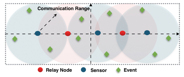
For second example, we consider a simple distributed self-localizing deployment problem concerned with optimal deployment of 33 sensors labeled Si\text{S}^{i}, i∈{1,3,5}i\in\{1,3,5\} on a line to monitor a set of events that are horizontally located at 𝐏=[{pi}i=110]=[12,11,9,3,2,−1,−2,−8,−11,−13]\boldsymbol{\mathbf{P}}\!=\![\{p_{i}\}_{i=1}^{10}]=[12,11,9,3,2,-1,-2,-8,-11,\\ -13] for t∈[0,100)t\in[0,100) , and 𝐏=[{pi}i=110]=[24,22,17,15,13,8,7,3,−2,−4]\boldsymbol{\mathbf{P}}\!=\![\{p_{i}\}_{i=1}^{10}]\!=\![24,22,17,15,\\ 13,8,7,3,-2,-4] for t∈[100,200)t\in[100,200), see Fig. 4. Agent 11 is monitoring {pi}i=13\{p_{i}\}_{i=1}^{3}, agent 33 is monitoring {pi}i=47\{p_{i}\}_{i=4}^{7}, and agent 55 is monitoring {pi}i=810\{p_{i}\}_{i=8}^{10}. Sensors should find their positions cooperatively to keep their position in the communication range of each other as well as stay close to the targets to improve the detection accuracy. Due to limited communication range, two relay nodes Ri\text{R}^{i}, i∈{2,4}i\in\{2,4\}, as shown in Fig. 4 are used to guarantee the connectivity of the sensors during the operation. The problem is formulated by

𝘅⋆=\displaystyle\boldsymbol{\mathbf{\mathsf{x}}}^{\star}= arg⁡min⁡∑i=15𝐱∈ℝ5⁡fi​(xi),subject to\displaystyle\arg\min_{\boldsymbol{\mathbf{x}}\in{\mathbb{R}}^{5}}\,\,\sum\nolimits_{i=1}^{5}f^{i}(x^{i}),~~\text{subject~to~} (24)
xj−xj+1≤5,j∈{1,⋯,4},\displaystyle~~~x^{j}-x^{j+1}\leq 5,\quad\quad j\in\{1,\cdots,4\},

where fi​(xi)=∑j∈Ei‖xi−pj‖2f^{i}(x^{i})=\sum_{j\in E^{i}}\|x^{i}-p_{j}\|^{2} for i∈{1,3,5}i\in\{1,3,5\} with E1={1,⋯,3}E^{1}=\{1,\cdots,3\}, E3={4,⋯,7}E^{3}=\{4,\cdots,7\} and E5={8,⋯,10}E^{5}=\{8,\cdots,10\} and fi​(xi)=0f^{i}(x^{i})=0 for i∈{2,4}i\in\{2,4\}. Here, xix^{i} with i∈{1,3,5}i\in\{1,3,5\} (resp. i∈{2,4}i\in\{2,4\}) is the horizontal position of sensor Si\text{S}^{i} (resp. relay node Ri\text{R}^{i}). To transform problem (24) to the standard form described in (1) we introduce slack variables x2i∈x^{i}_{2}\in\real with i∈{1,⋯,4}i\in\{1,\cdots,4\}, to rewrite (24) as

𝘅⋆=arg⁡min⁡∑i=15𝐱∈ℝ9⁡fi​(𝐱i),subject to\displaystyle\boldsymbol{\mathbf{\mathsf{x}}}^{\star}=\arg\min_{\boldsymbol{\mathbf{x}}\in{\mathbb{R}}^{9}}\,\,\sum\nolimits_{i=1}^{5}f^{i}(\boldsymbol{\mathbf{x}}^{i}),~~\text{subject~to~} (25)
x1j−x1j+1+x2j=5,x2j≥0,j∈{1,⋯,4},\displaystyle~x^{j}_{1}-x^{j+1}_{1}+x^{j}_{2}=5,~~x^{j}_{2}\geq 0,~~j\in\{1,\cdots,4\},

where 𝐱i∈2\boldsymbol{\mathbf{x}}^{i}\in\real^{2} for i∈{1,2,3,4}i\in\{1,2,3,4\}, 𝐱5∈\boldsymbol{\mathbf{x}}^{5}\in\real, and fi​(𝐱i)=fi​(x1i)f^{i}(\boldsymbol{\mathbf{x}}^{i})=f^{i}(x^{i}_{1}) for any i∈{1,⋯,5}i\in\{1,\cdots,5\}, i.e., fi​(x2i)=0f^{i}(x^{i}_{2})=0. We can run algorithm (7) by choosing the cyber layer equivalent to the physical connected topology between all the agent, i.e., 𝒢k=𝒢\mathcal{G}_{k}=\mathcal{G} for k∈{1,2,3,4}k\in\{1,2,3,4\}, where 𝒢\mathcal{G} is the line graph connecting all 55 agents. However, as stated earlier this configuration leads to extra computational and communication efforts. Here, instead, we form 44 cyber-layers 𝒢k\mathcal{G}_{k}, k∈{1,2,3,4}k\in\{1,2,3,4\}, where 𝒱1={1,2}\mathcal{V}_{1}=\{1,2\}, 𝒱2={2,3}\mathcal{V}_{2}=\{2,3\}, 𝒱3={3,4}\mathcal{V}_{3}=\{3,4\} and 𝒱4={4,5}\mathcal{V}_{4}=\{4,5\}. We note that our proposed approach to form the cyber-layers in correspondence to the equality constraints leads to an efficient communication topology here. More specifically, to generate the dual dynamics, the agents {1,⋯,5}\{1,\cdots,5\}, maintain and communicate variables of order {1,2,2,2,1}\{1,2,2,2,1\}, respectively. Whereas, if we implement algorithms of [19, 21], the corresponding variables to generate the dual dynamics is of order {8,8,8,8,4}\{8,8,8,8,4\}.

Refer to caption
Figure 4: Schematic representation of the events, sensors and relay nodes in the second example.

Figure 5 shows the trajectory of the distributed optimization algorithm (7) (using fpi​(𝐱1i)f^{i}_{\text{p}}(\boldsymbol{\mathbf{x}}_{1}^{i}) as defined in (12) in place of fi​(𝐱i)f^{i}(\boldsymbol{\mathbf{x}}^{i}) in (7c)) for problem (25). As shown the location of the sensors remain in their communication range and converge to optimum values during execution of the algorithm (the optimal solution is shown by the grey lines, and is obtained by MATLAB’s constraint optimization solver ‘fmincon’). Our choice of smooth penalty function (12) is obtained by γ=200\gamma=200 and ϵ=0.01\epsilon=0.01 which satisfies the condition of Proposition 3.1. What is interesting to note in Fig. 5 is how the convergence of the algorithm is slowed down when we use 𝒢k=𝒢\mathcal{G}_{k}=\mathcal{G} for k∈ℤ14k\in\mathbb{Z}_{1}^{4}. This is expected, as in this case the coordination to generate the dual variables has to happen over a larger graph.

Table 2 gives the global cost value and the inequality constraint evaluation at 𝘅p⋆\boldsymbol{\mathbf{\mathsf{x}}}_{p}^{\star} obtained by using our distributed algorithm with ϵ\epsilon-exact penalty function method for three simulation scenarios. The first and the second scenarios are respectively when we use ϵ=0.01\epsilon=0.01 and ϵ=0.001\epsilon=0.001. As we can see when ϵ=0.01\epsilon=0.01 only one of the inequalities is violated slightly (by 2.1​e−42.1\text{e}^{-4}). When a smaller ϵ=0.001\epsilon=0.001 is used this violation also is removed. Table 2 also shows that if we use the ’adjusted boxed inequalities’ that we introduced in Remark 3.3, the inequality constraints are all respected with only a negligible increase in the cost value.

Table 2: The global cost value and the inequality constraint evaluation at 𝘅p⋆\boldsymbol{\mathbf{\mathsf{x}}}_{p}^{\star} obtained by using ϵ\epsilon-exact penalty function method
x1−x2−5x^{1}-x^{2}-5 x2−x3−5x^{2}-x^{3}-5 x3−x4−5x^{3}-x^{4}-5 x4−x5−5x^{4}-x^{5}-5 f⁡(𝐱p⋆)f(\boldsymbol{\mathbf{x}}_{p}^{\star})
ϵ=0.01\epsilon=0.01 -5.8e-3 -2.06e-2 -2.63e-2 2.1e-4 680.4
ϵ=0.001\epsilon=0.001 -5.92-3 -3.46e-2 -3.75e-2 -3.5e-2 680.4
ϵ=0.01\epsilon=0.01 and adjusted bounds -1.25e-2 -1.3e-2 -3.92e-2 -8.2e-3 680.23
Figure 5: Trajectories of {x1i}i=15\{x_{1}^{i}\}_{i=1}^{5} generated by implementing distributed algorithm (7): The grey lines show the optimum positions of agents on the line obtained by using the Matlab’s fmincon. The thick curved lines show the trajectories when algorithm (7) is implemented over cluster-based cyber-layers. the thin lines show the trajectories when algorithm (7) is implemented with 𝒢k=𝒢\mathcal{G}_{k}=\mathcal{G}, k={1,2,3,4}k=\{1,2,3,4\}.

5 Conclusions

We proposed a novel cluster-based distributed augmented Lagrangian algorithm for a class of constrained convex optimization problem. In the design of our distributed algorithm, we paid special attention to the efficient communication and computation resource management and required only the agents that are coupled through an equality constraint to form a communication topology to address that coupling in a distributed manner. We showed that if the communication topology corresponding to each equality constraint is a connected graph, the proposed algorithm converges asymptotically when the local cost functions are convex, and exponentially when the local cost functions are strongly convex and have Lipschitz gradients. We invoked the ϵ\epsilon-exact penalty function method to address the inequality constraints and obtained an explicit lower bound on the penalty function weight to guarantee convergence to ϵ\epsilon-neighborhood of the global minimum value of the cost. Simulations demonstrated the performance of our proposed algorithm. As future work, we will study the event-triggered communication implementation of our algorithm.

References

  • [1] S. S. Kia, “An augmented lagrangian distributed algorithm for an in-network optimal resource allocation problem,” in American Control Conference, (WA, USA), 2017.
  • [2] A. J. Wood, F. Wollenberg, and G. B. Sheble, Power Generation, Operation and Control. New York: John Wiley, 3rd ed., 2013.
  • [3] A. Cherukuri and J. Cortés, “Initialization-free distributed coordination for economic dispatch under varying loads and generator commitment,” Automatica, vol. 74, pp. 183–193, 2016.
  • [4] L. Xiao, M. Johansson, and S. P. Boyd, “Simultaneous routing and resource allocation via dual decomposition,” IEEE Transactions on Communications, vol. 52, no. 7, pp. 1136–1144, 2004.
  • [5] R. Madan and S. Lall, “Distributed algorithms for maximum lifetime routing in wireless sensor networks,” IEEE Transactions on Wireless Communications, vol. 5, no. 8, pp. 2185–2193, 2006.
  • [6] J. Chen and V. K. N. Lau, “Convergence analysis of saddle point problems in time varying wireless systems – control theoretical approach,” IEEE Transactions on Signal Processing, vol. 60, no. 1, pp. 443–452, 2012.
  • [7] A. Ferragut and F. Paganini, “Network resource allocation for users with multiple connections: fairness and stability,” IEEE/ACM Transactions on Networking, vol. 22, no. 2, pp. 349–362, 2014.
  • [8] S. A. Alghunaim, K. Yuan, and A. H. Sayed, “Dual coupled diffusion for distributed optimization with affine constraints,” in IEEE Conf. on Decision and Control, (FL, USA), 2018.
  • [9] R. Rostami, G. Costantini, and D. Görges, “ADMM-based distributed model predictive control: Primal and dual approaches,” in IEEE Conf. on Decision and Control, (Melbourne, Australia), 2017.
  • [10] S. Boyd, N. Parikh, E. Chu, B. Peleato, and J. Eckstein, “Distributed optimization and statistical learning via the alternating direction method of multipliers,” Foundations and Trends in Machine Learning, vol. 3, pp. 1–122, 2010.
  • [11] J. Duchi, A. Agarwal, and M. Wainwright, “Dual averaging for distributed optimization: Convergence analysis and network scaling,” IEEE Transactions on Automatic Control, vol. 57, no. 3, pp. 592–606, 2012.
  • [12] J. Wang and N. Elia, “A control perspective for centralized and distributed convex optimization,” in IEEE Conf. on Decision and Control, (FL, USA), 2011.
  • [13] S. S. Kia, J. Cortés, and S. Martínez, “Distributed convex optimization via continuous-time coordination algorithms with discrete-time communication,” Automatica, vol. 55, pp. 254–264, 2014.
  • [14] D. Varagnolo, F. Zanella, A. Cenedese, G. Pillonetto, and L. Schenato, “Newton-raphson consensus for distributed convex optimization,” IEEE Transactions on Automatic Control, vol. 61, no. 4, pp. 994 – 1009, 2015.
  • [15] Z. Zhang and M. Chow, “Convergence analysis of the incremental cost consensus algorithm under different communication network topologies in a smart grid,” IEEE Transactions on Power Systems, vol. 27, no. 4, pp. 1761–1768, 2012.
  • [16] S. Kar and G. Hug, “Distributed robust economic dispatch in power systems: A consensus + innovations approach,” in Power & Energy Society General Meeting, (San Diego, CA), pp. 1–8, July 2012.
  • [17] A. D. Dominguez-Garcia, S. T. Cady, and C. N. Hadjicostis, “Decentralized optimal dispatch of distributed energy resources,” in IEEE Conf. on Decision and Control, (Hawaii, USA), pp. 3688–3693, Dec. 2012.
  • [18] L. Xiao and S. Boyd, “Optimal scaling of a gradient method for distributed resource allocation,” Journal of optimization theory and applications, vol. 129, no. 3, pp. 469–488, 2006.
  • [19] Y. Zhang and M. M. Zavlanos, “A consensus-based distributed augmented lagrangian method,” in IEEE Conf. on Decision and Control, (CA, USA), 2018.
  • [20] P. Yi, Y. Hong, and F. Liu, “Initialization-free distributed algorithms for optimal resource allocation with feasibility constraints and its application to economic dispatch of power systems,” Automatica, vol. 74, pp. 259–269, 2016.
  • [21] S. S. Kia, “Distributed optimal in-network resource allocation algorithm design via a control theoretic approach,” Systems and Control Letters, vol. 107, pp. 49–57, 2017.
  • [22] D. Ding and M. Jovanovic´, “A primal-dual Laplacian gradient flow dynamics for distributed resource allocation problems,” in American Control Conference, (WI, USA), 2018.
  • [23] A. Cherukuri and J. Cortés, “Initialization-free distributed coordination for economic dispatch under varying loads and generator commitment,” Automatica, vol. 74, pp. 183–193, 2016.
  • [24] A. Cherukuri and J. Cortés, “Distributed generator coordination for initialization and anytime optimization in economic dispatch,” IEEE Transactions on Control of Network Systems, vol. 2, no. 3, pp. 226–237, 2015.
  • [25] D. Bertsekas and J. Tsitsiklis, Parallel and Distributed Computation: Numerical Methods. 1997.
  • [26] D. Jakovetic, J. Moura, and J. Xavier, “Linear convergence rate of a class of distributed augmented lagrangian algorithms,” IEEE Transactions on Automatic Control, vol. 60, no. 4, pp. 922–936, 2015.
  • [27] M.Vaquero and J.Cortes, “Distributed augmentation-regularization for robust online convex optimization,” IFAC-PapersOnLine, vol. 51, no. 23, pp. 230–235, 2018.
  • [28] K. J. Arrow, L. Hurwicz, and H. Uzawa, Studies in linear and nonlinear programming. 1958.
  • [29] D. Ding, B. Hu, N. Dhingra, and M. Jovanovic´, “An exponentially convergent primal-dual algorithm for nonsmooth composite minimization,” in IEEE Conf. on Decision and Control, (FL, USA), 2018.
  • [30] S. S. Kia, “Distributed optimal resource allocation over networked systems and use of an epsilon-exact penalty function,” in IFAC Symposium on Large Scale Complex Systems, (CA, USA), 2016.
  • [31] W. Haddad and V. Chellaboina, Nonlinear Dynamical Systems and Control. Princeton University Press, 2008.
  • [32] D. P. Bertsekas, “Nondifferentiable optimization via approximation,” Mathematical Programing Study, vol. 3, pp. 1–25, 1975.
  • [33] M. Ç. Pinar and S. A. Zenios, “On smoothing exact penalty functions for convex constrained optimization,” IEEE Transactions on Communications, vol. 4, no. 3, pp. 1136–1144, 1994.
  • [34] W. Wei, J. Wang, N. Li, and S. Mei, “Optimal power flow of radial networks and its variations: A sequential convex optimization approach,” IEEE Transactions on Smart Grid, vol. 8, no. 6, pp. 2974–2987, 2017.
  • [35] M. Zholbaryssov, D. Fooladivanda, and A. D.Domínguez-García, “Resilient distributed optimal generation dispatch for lossy ac microgrids,” Systems and Control Letters, vol. 123, pp. 47–54, 2019.
  • [36] O. Mangasarian, “Computable numerical bounds for lagrange multipliers of stationary points of non-convex differentiable non-linear programs,” Operations Research Letters, vol. 4, no. 2, pp. 1757–1780, 1985.
  • [37] S. Richter, M. Morari, and C. Jones, “Towards computational complexity certification for constrained MPC based on Lagrange relaxation and the fast gradient method,” in IEEE Conf. on Decision and Control, (Orlando, Florida, USA), pp. 5223 – 5229, 2011.
  • [38] F. Bullo, J. Cortés, and S. Martínez, Distributed Control of Robotic Networks. Applied Mathematics Series, Princeton University Press, 2009.
  • [39] S. Boyd and L. Vandenberghe, Convex Optimization. Cambridge University Press, 2004.
  • [40] D. Bertsekas, Nonlinear Programming. 1999.
  • [41] O. L. Mangasarian and S. Fromovitz, “The fritz john necessary optimality conditions in the presence of equality and inequality constraints,” Operations Research Letters, vol. 17, pp. 37–47, 1967.
  • [42] G. Wachsmuth, “On LICQ and the uniqueness of Lagrange multipliers,” Operations Research Letters, vol. 41, no. 1, pp. 78–80, 2013.
  • [43] P. Srivastava and J. Cortes, “Distributed algorithm via continuously differentiable exact penalty method for network optimization,” in IEEE Conf. on Decision and Control, (FL, USA), 2018.
  • [44] 2004. http://motor.ece.iit.edu/data/JEAS\_IEEE118.doc.
  • [45] H. K. Khalil, Nonlinear Control. Prentice Hall, 2002.

Appendix A

PROOF.

[Proof of Theorem 3.1] Let ({𝘅i⋆}i=1N,𝝂⋆)(\{\boldsymbol{\mathbf{\mathsf{x}}}^{i\star}\}_{i=1}^{N},{\boldsymbol{\mathbf{\mathsf{\nu}}}}^{\star}) satisfy the KKT equation (5) and 𝐲k⋆=[{[𝘄l]k𝘅l⋆−𝖻¯kl}l∈𝒱k]\boldsymbol{\mathbf{y}}^{\star}_{k}=[\{[\boldsymbol{\mathbf{\mathsf{w}}}^{l}]_{k}\boldsymbol{\mathbf{\mathsf{x}}}^{l\star}-\bar{\mathsf{b}}^{l}_{k}\}_{l\in\mathcal{V}_{k}}]. For convenience in analysis, we apply the change of variables

𝐪k\displaystyle\!\!\boldsymbol{\mathbf{q}}_{k}\! =[𝗿k⊤𝗥k⊤](𝐲k−𝐲k⋆),𝐩k=𝐯k−νk⋆𝟏Nk,𝝌i=𝐱i−𝘅i⋆,\displaystyle=\!\begin{bmatrix}\boldsymbol{\mathbf{\mathsf{r}}}_{k}^{\top}\!\\ \boldsymbol{\mathbf{\mathsf{R}}}_{k}^{\top}\!\end{bmatrix}\!(\boldsymbol{\mathbf{y}}_{k}\!-\!\boldsymbol{\mathbf{y}}^{\star}_{k}),\,\,\boldsymbol{\mathbf{p}}_{k}\!=\!\boldsymbol{\mathbf{v}}_{k}\!-\!\nu^{\star}_{k}\boldsymbol{\mathbf{1}}_{N_{k}},\,\boldsymbol{\mathbf{\chi}}^{i}=\boldsymbol{\mathbf{x}}^{i}\!-\!\boldsymbol{\mathbf{\mathsf{x}}}^{i\star}, (A.26)

to write the algorithm (7), under the stated initialization conditions, in the equivalent form

q^˙k=\displaystyle\dot{\hat{q}}_{k}=  0,\displaystyle\,0, (A.27a)
𝐪¯.k=\displaystyle\overset{.}{\bar{\boldsymbol{\mathbf{q}}}}_{k}= βk​(𝗥k⊤​𝗟k​𝗥k)​𝗥k⊤​𝐩k,\displaystyle\,\beta_{k}\,(\boldsymbol{\mathbf{\mathsf{R}}}_{k}^{\top}\boldsymbol{\mathbf{\mathsf{L}}}_{k}\boldsymbol{\mathbf{\mathsf{R}}}_{k})\,\boldsymbol{\mathbf{\mathsf{R}}}_{k}^{\top}\boldsymbol{\mathbf{p}}_{k}, (A.27b)
𝐩˙k=\displaystyle\dot{\boldsymbol{\mathbf{p}}}_{k}= 𝝍k​𝝌k−βk​𝗟k​𝐩k−𝗥k​𝐪¯k−𝗿k​q^k,\displaystyle\,\boldsymbol{\mathbf{\mathsf{\psi}}}_{k}\boldsymbol{\mathbf{\chi}}_{k}-\beta_{k}\,\boldsymbol{\mathbf{\mathsf{L}}}_{k}\boldsymbol{\mathbf{p}}_{k}-\boldsymbol{\mathbf{\mathsf{R}}}_{k}\,\bar{\boldsymbol{\mathbf{q}}}_{k}-\boldsymbol{\mathbf{\mathsf{r}}}_{k}\,\hat{q}_{k}, (A.27c)
𝝌˙i=\displaystyle\dot{\boldsymbol{\mathbf{\chi}}}^{i}= −(ρi+1)(∇fi(𝝌i+𝘅i⋆)−∇fi(𝘅i⋆))+\displaystyle\,-(\rho^{i}+1)\,(\nabla f^{i}(\boldsymbol{\mathbf{\chi}}^{i}+{\boldsymbol{\mathbf{\mathsf{x}}}}^{i\star})-\nabla f^{i}({\boldsymbol{\mathbf{\mathsf{x}}}}^{i\star}))\,+\,
∑k∈𝒯i(−ρi​[𝘄i]k⊤​[𝘄i]k​𝝌i−(ρi+1)​[𝘄i]k⊤​pkiCLOSE\displaystyle\sum\nolimits_{k\in\mathcal{T}^{i}}\big(-\rho^{i}[\boldsymbol{\mathbf{\mathsf{w}}}^{i}]_{k}^{\top}[\boldsymbol{\mathbf{\mathsf{w}}}^{i}]_{k}\boldsymbol{\mathbf{\chi}}^{i}\,-(\rho^{i}+1)[\boldsymbol{\mathbf{\mathsf{w}}}^{i}]^{\top}_{k}p_{k}^{i}
OPEN+ρi​[𝘄i]k⊤​[𝗥k​𝐪¯k]i+ρi​[𝘄i]k⊤​q^k),\displaystyle+\rho^{i}{[\boldsymbol{\mathbf{\mathsf{w}}}}^{i}]^{\top}_{k}[\boldsymbol{\mathbf{\mathsf{R}}}_{k}\,\bar{\boldsymbol{\mathbf{q}}}_{k}]^{i}+\rho^{i}\,{[\boldsymbol{\mathbf{\mathsf{w}}}}^{i}]^{\top}_{k}\!\,\hat{q}_{k}\big), (A.27d)

where we used 𝐪k=(q^k,𝐪¯k)\boldsymbol{\mathbf{q}}_{k}=(\hat{q}_{k},\bar{\boldsymbol{\mathbf{q}}}_{k}) with q^k∈,𝐪¯k∈(Nk−1)\hat{q}_{k}\in\!\real,\,\bar{\boldsymbol{\mathbf{q}}}_{k}\in\!\real^{(N_{k}-1)}. Here, we also used 𝗥k​𝗥k⊤​𝗟k=𝗟k\boldsymbol{\mathbf{\mathsf{R}}}_{k}\boldsymbol{\mathbf{\mathsf{R}}}_{k}^{\top}\boldsymbol{\mathbf{\mathsf{L}}}_{k}=\boldsymbol{\mathbf{\mathsf{L}}}_{k}, 𝝍k=Blkdiag​({[𝘄i]k}i∈𝒱k)\boldsymbol{\mathbf{\mathsf{\psi}}}_{k}=\text{Blkdiag}(\{[\boldsymbol{\mathbf{\mathsf{w}}}^{i}]_{k}\}_{i\in\mathcal{V}_{k}}) and 𝝌k=[{𝝌i⊤}i∈𝒱k]⊤\boldsymbol{\mathbf{\chi}}_{k}=[\{\boldsymbol{\mathbf{\chi}}^{i\top}\}_{i\in\mathcal{V}_{k}}]^{\top}. Under the given initial condition, for any t∈ℝ≥0t\in{\mathbb{R}}_{\geq 0} we obtain

q^k​(t)=1Nk​(∑l∈𝒱kykl​(t)−([𝗪]k​𝘅⋆−𝖻k))=0.\displaystyle\hat{q}_{k}(t)=\!\frac{1}{\sqrt{N_{k}}}\big(\sum\nolimits_{l\in\mathcal{V}_{k}}\!\!y_{k}^{l}(t)\!-\!\!([\boldsymbol{\mathbf{\mathsf{W}}}]_{k}\boldsymbol{\mathbf{\mathsf{x}}}^{\star}\!-\!\mathsf{b}_{k})\big)\!=\!0. (A.28)

To study the stability in the other variables, we let q^k​(t)=0\hat{q}_{k}(t)=0 in (A.27c) and (A.27d), and consider the radially unbounded candidate Lyapunov function

V⁡({𝐪¯k}k=1p,{𝐩k}k=1p,{𝝌i}i=1N)=12​∑i=1N𝝌i⊤​𝝌i+\displaystyle V(\{\bar{\boldsymbol{\mathbf{q}}}_{k}\}_{k=1}^{p},\{\boldsymbol{\mathbf{p}}_{k}\}_{k=1}^{p},\{\boldsymbol{\mathbf{\chi}}^{i}\}_{i=1}^{N})=\frac{1}{2}\sum\nolimits_{i=1}^{N}\boldsymbol{\mathbf{\chi}}^{i\top}\boldsymbol{\mathbf{\chi}}^{i}\,+
12​∑k=1p(𝐪¯k⊤​(𝚪k+𝗜)​(βk​𝗥k⊤​𝗟k​𝗥k)−1​𝐪¯k+𝐩k⊤​𝐩kCLOSE\displaystyle\quad\frac{1}{2}\sum\nolimits_{k=1}^{p}\big(\bar{\boldsymbol{\mathbf{q}}}_{k}^{\top}(\boldsymbol{\mathbf{\Gamma}}_{k}+\boldsymbol{\mathbf{\mathsf{I}}})(\beta_{k}\boldsymbol{\mathbf{\mathsf{R}}}_{k}^{\top}\boldsymbol{\mathbf{\mathsf{L}}}_{k}\boldsymbol{\mathbf{\mathsf{R}}}_{k})^{-1}\bar{\boldsymbol{\mathbf{q}}}_{k}+\boldsymbol{\mathbf{p}}^{\top}_{k}\boldsymbol{\mathbf{p}}_{k}
OPEN+(𝐩k+𝗥k​𝐪¯k)⊤​𝚪k​(𝐩k+𝗥k​𝐪¯k)),\displaystyle\qquad+(\boldsymbol{\mathbf{p}}_{k}+\boldsymbol{\mathbf{\mathsf{R}}}_{k}\,\bar{\boldsymbol{\mathbf{q}}}_{k})^{\top}\boldsymbol{\mathbf{\Gamma}}_{k}\,(\boldsymbol{\mathbf{p}}_{k}+\boldsymbol{\mathbf{\mathsf{R}}}_{k}\,\bar{\boldsymbol{\mathbf{q}}}_{k})\big), (A.29)

where 𝚪k=Blkdiag​({ρi}i∈𝒱k)\boldsymbol{\mathbf{\Gamma}}_{k}\!=\!\text{Blkdiag}(\{\rho^{i}\}_{i\in\mathcal{V}_{k}}). Note that (βk​𝗥k⊤​𝗟k​𝗥k)−1(\beta_{k}\boldsymbol{\mathbf{\mathsf{R}}}_{k}^{\top}\boldsymbol{\mathbf{\mathsf{L}}}_{k}\boldsymbol{\mathbf{\mathsf{R}}}_{k})^{-1} and 𝚪k+𝗜\boldsymbol{\mathbf{\Gamma}}_{k}+\boldsymbol{\mathbf{\mathsf{I}}} are positive definite diagonal matrices, thus 𝐪¯k⊤​(𝚪k+𝗜)​(βk​𝗥k⊤​𝗟k​𝗥k)−1​𝐪¯k>𝟎\bar{\boldsymbol{\mathbf{q}}}_{k}^{\top}(\boldsymbol{\mathbf{\Gamma}}_{k}+\boldsymbol{\mathbf{\mathsf{I}}})(\beta_{k}\boldsymbol{\mathbf{\mathsf{R}}}_{k}^{\top}\boldsymbol{\mathbf{\mathsf{L}}}_{k}\boldsymbol{\mathbf{\mathsf{R}}}_{k})^{-1}\bar{\boldsymbol{\mathbf{q}}}_{k}\!>\!\boldsymbol{\mathbf{0}}. Taking the derivative of VV along the trajectories of (A.27b)-(A.27d) gives

V˙=−∑i=1N((ρi+1)𝝌i⊤(∇f(𝝌i+𝘅i⋆)−∇f(𝘅i⋆))\displaystyle\!\dot{V}\!=\!-\!\!\sum\nolimits_{i=1}^{N}\!\big((\rho^{i}+1)\boldsymbol{\mathbf{\chi}}^{i\top}(\nabla f(\boldsymbol{\mathbf{\chi}}^{i}+{\boldsymbol{\mathbf{\mathsf{x}}}}^{i\star})-\!\nabla f({\boldsymbol{\mathbf{\mathsf{x}}}}^{i\star})) (A.30)
−∑k=1p(βk𝐩k⊤𝗟k𝐩k+(𝝍k𝝌k−𝗥k𝐪¯k)⊤𝚪k(𝝍k𝝌k−𝗥k𝐪¯k)).\displaystyle\!-\!\sum_{k=1}^{p}\!\!\big(\beta_{k}\,\boldsymbol{\mathbf{p}}_{k}^{\top}\boldsymbol{\mathbf{\mathsf{L}}}_{k}\boldsymbol{\mathbf{p}}_{k}\!+\!(\boldsymbol{\mathbf{\mathsf{\psi}}}_{k}\,\boldsymbol{\mathbf{\chi}}_{k}\!-\!\boldsymbol{\mathbf{\mathsf{R}}}_{k}\bar{\boldsymbol{\mathbf{q}}}_{k})^{\top}\!\boldsymbol{\mathbf{\Gamma}}_{k}\!(\boldsymbol{\mathbf{\mathsf{\psi}}}_{k}\boldsymbol{\mathbf{\chi}}_{k}\!-\!\boldsymbol{\mathbf{\mathsf{R}}}_{k}\bar{\boldsymbol{\mathbf{q}}}_{k})\big).

Convexity of the local cost functions ensures 𝝌i(∇fi(𝝌i+𝘅i⋆)−∇fi(𝘅i⋆))=((𝝌i+𝘅i⋆)−𝘅i⋆)(∇fi(𝝌i+𝘅i⋆)−∇fi(𝘅i⋆))≥0\boldsymbol{\mathbf{\chi}}^{i}(\boldsymbol{\mathbf{\nabla}}f^{i}(\boldsymbol{\mathbf{\chi}}^{i}+{\boldsymbol{\mathbf{\mathsf{x}}}}^{i\star})-\boldsymbol{\mathbf{\nabla}}f^{i}({\boldsymbol{\mathbf{\mathsf{x}}}}^{i\star}))=((\boldsymbol{\mathbf{\chi}}^{i}+{\boldsymbol{\mathbf{\mathsf{x}}}}^{i\star})-{\boldsymbol{\mathbf{\mathsf{x}}}}^{i\star})(\boldsymbol{\mathbf{\nabla}}f^{i}(\boldsymbol{\mathbf{\chi}}^{i}+{\boldsymbol{\mathbf{\mathsf{x}}}}^{i\star})-\boldsymbol{\mathbf{\nabla}}f^{i}({\boldsymbol{\mathbf{\mathsf{x}}}}^{i\star}))\geq 0, i∈𝒱i\in\mathcal{V}. The connectivity of the sub-graph 𝒢k\mathcal{G}_{k}, k∈ℤ1pk\in\mathbb{Z}_{1}^{p} also ensures −𝐩k⊤​𝗟k​𝐩k≤0-\boldsymbol{\mathbf{p}}_{k}^{\top}\boldsymbol{\mathbf{\mathsf{L}}}_{k}\boldsymbol{\mathbf{p}}_{k}\leq 0. Thus, V˙≤0\dot{V}\leq 0, and consequently the trajectories of (A.27b)-(A.27d) starting from any initial condition are bounded.

Next, we invoke the invariant set stability results to prove that the trajectories of (A.27b)-(A.27d) converge to a point in its set of equilibrium points. Let 𝒮={({𝐪¯k}k=1p,{𝐩k}k=1p,{𝝌i}i=1N)∈∏k=1p×Nk−1∏k=1p×Nk∏i=1Nℝni|V˙≡0}\mathcal{S}=\{(\{\bar{\boldsymbol{\mathbf{q}}}_{k}\}_{k=1}^{p},\{\boldsymbol{\mathbf{p}}_{k}\}_{k=1}^{p},\{\boldsymbol{\mathbf{\chi}}^{i}\}_{i=1}^{N})\in\prod_{k=1}^{p}\!\real{}^{N_{k}-1}\times\prod_{k=1}^{p}\!\real{}^{N_{k}}\times\prod_{i=1}^{N}{\mathbb{R}}^{n^{i}}|\,\dot{V}\equiv 0\}. Given (A.30), we have 𝒮={{𝐪¯k}k=1p,{𝐩k}k=1p,{𝝌i}i=1N∈∏k=1p×Nk−1∏k=1p×Nk∏i=1Nℝni|𝐩k=𝟎,𝝍k𝝌k=𝗥k𝐪¯k,𝝌i⊤(∇fi(𝝌i+𝘅i⋆)−∇fi(𝘅i⋆))=0,i∈𝒱,k∈ℤ1p}\mathcal{S}=\Big\{\!\{\bar{\boldsymbol{\mathbf{q}}}_{k}\}_{k=1}^{p},\!\{\boldsymbol{\mathbf{p}}_{k}\}_{k=1}^{p},\!\{\boldsymbol{\mathbf{\chi}}^{i}\}_{i=1}^{N}\!\in\!\prod_{k=1}^{p}\real{}^{N_{k}-1}\!\times\!\prod_{k=1}^{p}\real{}^{N_{k}}\times\prod_{i=1}^{N}{\mathbb{R}}^{n^{i}}\Big|~\boldsymbol{\mathbf{p}}_{k}=\boldsymbol{\mathbf{0}},~\boldsymbol{\mathbf{\mathsf{\psi}}}_{k}\,\boldsymbol{\mathbf{\chi}}_{k}=\boldsymbol{\mathbf{\mathsf{R}}}_{k}\bar{\boldsymbol{\mathbf{q}}}_{k},\\ \boldsymbol{\mathbf{\chi}}^{i\top}(\nabla f^{i}(\boldsymbol{\mathbf{\chi}}^{i}+{\boldsymbol{\mathbf{\mathsf{x}}}}^{i\star})-\nabla f^{i}({\boldsymbol{\mathbf{\mathsf{x}}}}^{i\star}))=0,~i\in\mathcal{V},~k\in\mathbb{Z}_{1}^{p}\big\}. Since 𝝌i⊤(∇fi(𝝌i+𝘅i⋆)−∇fi(𝘅i⋆))=∑j=1niχji(∇fji(χji+𝗑ji⋆)−∇fji(𝗑ji⋆))\boldsymbol{\mathbf{\chi}}^{i\top}(\nabla f^{i}(\boldsymbol{\mathbf{\chi}}^{i}+{\boldsymbol{\mathbf{\mathsf{x}}}}^{i\star})-\nabla f^{i}({\boldsymbol{\mathbf{\mathsf{x}}}}^{i\star}))=\sum_{j=1}^{n^{i}}\chi^{i}_{j}(\nabla f^{i}_{j}({\chi^{i}_{j}}+\mathsf{x}^{i\star}_{j})-\nabla f^{i}_{j}(\mathsf{x}^{i\star}_{j})), due to convexity of the cost functions fjif^{i}_{j}, j∈ℤ1nij\in\mathbb{Z}_{1}^{n_{i}}, i∈𝒱i\in\mathcal{V}, from 𝝌i⊤(∇fi(𝝌i+𝘅i⋆)−∇fi(𝘅i⋆))=0\boldsymbol{\mathbf{\chi}}^{i\top}(\nabla f^{i}(\boldsymbol{\mathbf{\chi}}^{i}+{\boldsymbol{\mathbf{\mathsf{x}}}}^{i\star})-\nabla f^{i}({\boldsymbol{\mathbf{\mathsf{x}}}}^{i\star}))=0 we conclude that either χji=0{\chi}_{j}^{i}=0 or ∇fji(χji+𝗑ji⋆))−∇fji(𝗑ji⋆))=0\nabla f_{j}^{i}({\chi^{i}_{j}}+\mathsf{x}^{i\star}_{j}))-\nabla f_{j}^{i}(\mathsf{x}^{i\star}_{j}))=0. Consequently, the points in 𝒮\mathcal{S} satisfy ∇fi(𝝌i+𝘅i⋆)−∇fi(𝘅i⋆)=0\nabla f^{i}(\boldsymbol{\mathbf{\chi}}^{i}+{\boldsymbol{\mathbf{\mathsf{x}}}}^{i\star})-\nabla f^{i}({\boldsymbol{\mathbf{\mathsf{x}}}}^{i\star})=0. As a result, given (A.28), a trajectory t↦({𝐪¯k​(t)}k=1p,{𝐩k​(t)}k=1p,{𝝌i​(t)}i=1N)t\mapsto(\{\bar{\boldsymbol{\mathbf{q}}}_{k}(t)\}_{k=1}^{p},\{\boldsymbol{\mathbf{p}}_{k}(t)\}_{k=1}^{p},\{\boldsymbol{\mathbf{\chi}}^{i}(t)\}_{i=1}^{N}) of (A.27b)-(A.27d) belonging to 𝒮\mathcal{S} for all t≥0t\geq 0, must satisfy (𝐪¯.k≡𝟎,𝐩˙k≡𝟎,𝝌˙i≡𝟎)(\overset{.}{\bar{\boldsymbol{\mathbf{q}}}}_{k}\equiv\boldsymbol{\mathbf{0}},\dot{\boldsymbol{\mathbf{p}}}_{k}\equiv\boldsymbol{\mathbf{0}},\dot{\boldsymbol{\mathbf{\chi}}}^{i}\equiv\boldsymbol{\mathbf{0}}). Therefore, the largest invariant set in 𝒮\mathcal{S} is the set of equilibrium points of (A.27b)-(A.27d). Then, invoking the La Salle invariant theorem  [31, Theorem 3.4], we conclude that the trajectories of (A.27b)-(A.27d) converge asymptotically to the set of its equilibrium points.

Next, we show that the convergence is indeed to a point in the equlibia set. For that, by virtue of semi-stability theorem [31, Theorem 4.20], we show that every equilibrium point of  (A.27b)-(A.27d) is Lyapunov stable. Let ({𝐪¯¯k}k=1p,{𝐩¯k},{𝝌¯i)}i=1N(\{\underline{\boldsymbol{\mathbf{\bar{q}}}\mkern-2.0mu}\mkern 2.0mu_{k}\}_{k=1}^{p},\{\underline{\boldsymbol{\mathbf{p}}\mkern-2.0mu}\mkern 2.0mu_{k}\},\{\underline{\boldsymbol{\mathbf{\chi}}\mkern-2.0mu}\mkern 2.0mu^{i})\}_{i=1}^{N} be an equilibrium point of  (A.27b)-(A.27d) (recall that q^k​(t)=0\hat{q}_{k}(t)=0 due to (A.28)). Now, consider the change of variables 𝔮k=𝐪¯k−𝐪¯¯k\mathbf{\mathfrak{q}}_{k}=\bar{\boldsymbol{\mathbf{q}}}_{k}-\underline{\boldsymbol{\mathbf{\bar{q}}}\mkern-2.0mu}\mkern 2.0mu_{k} and 𝔭k=𝐩k−𝐩¯k\mathbf{\mathfrak{p}}_{k}=\boldsymbol{\mathbf{p}}_{k}-\underline{\boldsymbol{\mathbf{p}}\mkern-2.0mu}\mkern 2.0mu_{k} for k∈ℤ1pk\in\mathbb{Z}_{1}^{p}, and 𝔯i=𝝌i−𝝌¯i\mathbf{\mathfrak{r}}^{i}=\boldsymbol{\mathbf{\chi}}^{i}-\underline{\boldsymbol{\mathbf{\chi}}\mkern-2.0mu}\mkern 2.0mu^{i} for i∈𝒱i\in\mathcal{V}, to write (A.27b)-(A.27d) as

𝔮˙k=\displaystyle\dot{\mathbf{\mathfrak{q}}}_{k}= βk​(𝗥k⊤​𝗟k​𝗥k)​𝗥k⊤​𝔭k,\displaystyle\,\beta_{k}\,(\boldsymbol{\mathbf{\mathsf{R}}}_{k}^{\top}\boldsymbol{\mathbf{\mathsf{L}}}_{k}\boldsymbol{\mathbf{\mathsf{R}}}_{k})\,\boldsymbol{\mathbf{\mathsf{R}}}_{k}^{\top}\mathbf{\mathfrak{p}}_{k}, (A.31a)
𝔭˙k=\displaystyle\dot{\mathbf{\mathfrak{p}}}_{k}= 𝝍k​𝔯k−βk​𝗟k​𝔭k−𝗥k​𝔮k,\displaystyle\,\boldsymbol{\mathbf{\mathsf{\psi}}}_{k}\mathbf{\mathfrak{r}}_{k}-\beta_{k}\,\boldsymbol{\mathbf{\mathsf{L}}}_{k}\mathbf{\mathfrak{p}}_{k}-\boldsymbol{\mathbf{\mathsf{R}}}_{k}\,\mathbf{\mathfrak{q}}_{k}, (A.31b)
𝔯˙i=\displaystyle\dot{\mathbf{\mathfrak{r}}}^{i}= −(ρi+1)(∇fi(𝔯i+𝝌¯i+𝘅i⋆)−∇fi(𝘅i⋆))+\displaystyle\,-(\rho^{i}+1)\,(\nabla f^{i}(\mathbf{\mathfrak{r}}^{i}+\underline{\boldsymbol{\mathbf{\chi}}\mkern-2.0mu}\mkern 2.0mu^{i}+{\boldsymbol{\mathbf{\mathsf{x}}}}^{i\star})-\nabla f^{i}({\boldsymbol{\mathbf{\mathsf{x}}}}^{i\star}))\,+\,
∑k∈𝒯i(−ρi​[𝘄i]k⊤​[𝘄i]k​𝔯i−(ρi+1)​[𝘄i]k⊤​𝔭kiCLOSE\displaystyle\sum\nolimits_{k\in\mathcal{T}^{i}}\big(-\rho^{i}[\boldsymbol{\mathbf{\mathsf{w}}}^{i}]_{k}^{\top}[\boldsymbol{\mathbf{\mathsf{w}}}^{i}]_{k}\mathbf{\mathfrak{r}}^{i}\,-(\rho^{i}+1)[\boldsymbol{\mathbf{\mathsf{w}}}^{i}]^{\top}_{k}\mathfrak{p}_{k}^{i}
OPEN+ρi​[𝘄i]k⊤​[𝗥k​𝔮k]i).\displaystyle+\rho^{i}{[\boldsymbol{\mathbf{\mathsf{w}}}}^{i}]^{\top}_{k}[\boldsymbol{\mathbf{\mathsf{R}}}_{k}\,\mathbf{\mathfrak{q}}_{k}]^{i}\big). (A.31c)

Next, consider the Lyapunov function (PROOF.) where ({𝐪¯k}k=1p,{𝐩k}k=1p,{𝝌i}i=1N)(\{\bar{\boldsymbol{\mathbf{q}}}_{k}\}_{k=1}^{p},\{\boldsymbol{\mathbf{p}}_{k}\}_{k=1}^{p},\{\boldsymbol{\mathbf{\chi}}^{i}\}_{i=1}^{N}) is substituted by ({𝔮k}k=1p,{𝔭k}k=1p,{𝔯i}i=1N)(\{\mathbf{\mathfrak{q}}_{k}\}_{k=1}^{p},\\ \{\mathbf{\mathfrak{p}}_{k}\}_{k=1}^{p},\{\mathbf{\mathfrak{r}}^{i}\}_{i=1}^{N}). Following the same argument used to show V˙≤0\dot{V}\leq 0 in (A.30), we can show that the derivative of V⁡({𝔮k}k=1p,{𝔭k}k=1p,{𝔯i}i=1N)V(\{\mathbf{\mathfrak{q}}_{k}\}_{k=1}^{p},\{\mathbf{\mathfrak{p}}_{k}\}_{k=1}^{p},\{\mathbf{\mathfrak{r}}^{i}\}_{i=1}^{N}) along the trajectories of (A.27b)-(A.27d), when (A.28) holds, is also negative semi-definite. Thus, any equilibrium point ({𝐪¯¯k}k=1p,{𝐩¯k},{𝝌¯i}i=1N)(\{\underline{\bar{\boldsymbol{\mathbf{q}}}\mkern-2.0mu}\mkern 2.0mu_{k}\}_{k=1}^{p},\{\underline{\boldsymbol{\mathbf{p}}\mkern-2.0mu}\mkern 2.0mu_{k}\},\{\underline{\boldsymbol{\mathbf{\chi}}\mkern-2.0mu}\mkern 2.0mu^{i}\}_{i=1}^{N}) of (A.27b)-(A.27d) is Lyapunov stable (recall (A.28)). Therefore, since the trajectories of (A.27b)-(A.27d) are approaching to the set of stable equilibrium points, starting from any initial condition, the trajectories of (A.27b)-(A.27d) converge to a point in its equilibrium set. Consequently, given the change of variables (A.26), we conclude that starting from stated initial conditions in the statement, the trajectories of (7) converge, as t→∞t\to\infty, to a point in its set of equilibrium points (3), where ({v˙kl}l∈𝒱k=𝟎,{y˙kl}l∈𝒱k=𝟎,{𝐱˙i}i=1N=𝟎)(\{\dot{v}^{l}_{k}\}_{l\in\mathcal{V}_{k}}=\boldsymbol{\mathbf{0}},\{\dot{y}^{l}_{k}\}_{l\in\mathcal{V}_{k}}=\boldsymbol{\mathbf{0}},\{\dot{\boldsymbol{\mathbf{x}}}^{i}\}_{i=1}^{N}=\boldsymbol{\mathbf{0}}). Therefore, under the stated initial condition, as t→∞t\to\infty, the limit point ({vkl}k=1p,{ykl}k=1p,{𝐱i}i=1N)(\{{v}^{l}_{k}\}_{k=1}^{p},\{{y}^{l}_{k}\}_{k=1}^{p},\{\boldsymbol{\mathbf{x}}^{i}\}_{i=1}^{N}), i∈𝒱i\in\mathcal{V}, l∈𝒱kl\in\mathcal{V}_{k} that satisfies ({v˙kl}l∈𝒱k=𝟎,{y˙kl}l∈𝒱k=𝟎,{𝐱˙i}i=1N=𝟎)(\{\dot{v}^{l}_{k}\}_{l\in\mathcal{V}_{k}}=\boldsymbol{\mathbf{0}},\{\dot{y}^{l}_{k}\}_{l\in\mathcal{V}_{k}}=\boldsymbol{\mathbf{0}},\{\dot{\boldsymbol{\mathbf{x}}}^{i}\}_{i=1}^{N}=\boldsymbol{\mathbf{0}}) in (7) is equal to (νk⋆𝟏Nk,𝘆⋆,{𝘅i⋆}i=1N)(\nu^{\star}_{k}\boldsymbol{\mathbf{1}}_{N_{k}},\boldsymbol{\mathbf{\mathsf{y}}}^{\star},\{\boldsymbol{\mathbf{\mathsf{x}}}^{i\star}\}_{i=1}^{N}), where ({νk⋆}k=1p,𝘅i⋆)(\{\nu^{\star}_{k}\}_{k=1}^{p},\boldsymbol{\mathbf{\mathsf{x}}}^{i\star}), where ({νk⋆}k=1p,{𝘅i⋆}i=1N)(\{{\nu}_{k}^{\star}\}_{k=1}^{p},\{{\boldsymbol{\mathbf{\mathsf{x}}}^{i\star}}\}_{i=1}^{N}) is a point satisfying the KKT conditions (5) of problem (4) (this point is not necessarily the point used in the change of variable (A.26)).

PROOF.

[Proof of Theorem 3.2] Follow the proof of Theorem 3.1 until the choice of the candidate Lyapounv function where we use the candidate function below consisted of VV in (PROOF.) plus an extra positive quadratic term

V¯​({𝐪¯k}k=1p,{𝐩k}k=1p,{𝝌i}i=1N)=V+\displaystyle\bar{V}(\{\bar{\boldsymbol{\mathbf{q}}}_{k}\}_{k=1}^{p},\{\boldsymbol{\mathbf{p}}_{k}\}_{k=1}^{p},\{\boldsymbol{\mathbf{\chi}}^{i}\}_{i=1}^{N})=V+
∑k=1pϕk2​(𝝌k+𝝍k⊤​𝚪k​𝐩k)⊤​(𝝌k+𝝍k⊤​𝚪k​𝐩k)=𝜻⊤​𝐄​𝜻,\displaystyle\quad\sum\nolimits^{p}_{k=1}\frac{\phi_{k}}{2}(\boldsymbol{\mathbf{\chi}}_{k}+\boldsymbol{\mathbf{\mathsf{\psi}}}_{k}^{\top}\boldsymbol{\mathbf{\Gamma}}_{k}\boldsymbol{\mathbf{p}}_{k})^{\top}\!(\boldsymbol{\mathbf{\chi}}_{k}\!+\!\boldsymbol{\mathbf{\mathsf{\psi}}}_{k}^{\top}\boldsymbol{\mathbf{\Gamma}}_{k}\boldsymbol{\mathbf{p}}_{k})=\boldsymbol{\mathbf{\zeta}}^{\top}\boldsymbol{\mathbf{E}}\boldsymbol{\mathbf{\zeta}},

where ϕk∈ℝ>0\phi_{k}\in{\mathbb{R}}_{>0} satisfies ϕk<min⁡{2​(1+ρ¯)​mp⁡(M2​(ρ¯2+1)2+1),2​βk​λ2​k(βk2​λN​k2​ρ¯2+ρ¯+1)​‖𝝍k‖2},\phi_{k}<\min\{\frac{2(1+\underline{\rho})m}{p(M^{2}(\bar{\rho}^{2}+1)^{2}\!+1)},\\ \frac{2\beta_{k}\lambda_{2k}}{(\beta^{2}_{k}\lambda_{Nk}^{2}\bar{\rho}^{2}+\bar{\rho}+1)\|\boldsymbol{\mathbf{\psi}}_{k}\|^{2}}\}, with ρ¯=min⁡{ρi}i=1N\underline{\rho}=\min\{\rho^{i}\}_{i=1}^{N} and ρ¯=max⁡{ρi}i=1N\bar{\rho}=\max\{\rho^{i}\}_{i=1}^{N}. Here 𝜻=[{𝐪¯k⊤}k=1p,{𝐩k⊤}k=1p,{𝝌i⊤}i=1N]⊤\boldsymbol{\mathbf{\zeta}}=[\{\bar{\boldsymbol{\mathbf{q}}}_{k}^{\top}\}_{k=1}^{p},\{\boldsymbol{\mathbf{p}}_{k}^{\top}\}_{k=1}^{p},\{\boldsymbol{\mathbf{\chi}}^{i\top}\}_{i=1}^{N}]^{\top} and 𝐄>0\boldsymbol{\mathbf{E}}>0 is the obvious matrix describing the coefficients of the quadratic terms of V¯\bar{V}. When every 𝒢k\mathcal{G}_{k}, k∈ℤ1pk\in\mathbb{Z}_{1}^{p} is a connected graph, V¯\bar{V} is a radially unbounded and positive definite function. Then,

V¯˙=\displaystyle\dot{\bar{V}}= −∑i=1N(ρi+1)𝝌i⊤𝐡(𝝌i)+∑k=1p(−βk𝐩k⊤𝗟k𝐩k\displaystyle-\!\sum\nolimits_{i=1}^{N}(\rho^{i}+1){\boldsymbol{\mathbf{\chi}}^{i}}^{\top}\boldsymbol{\mathbf{h}}(\boldsymbol{\mathbf{\chi}}^{i})\!+\!\sum\nolimits_{k=1}^{p}\Big(\!-\beta_{k}\boldsymbol{\mathbf{p}}_{k}^{\top}\boldsymbol{\mathbf{\mathsf{L}}}_{k}\boldsymbol{\mathbf{p}}_{k}
−(𝝍k​𝝌k−𝗥k​𝐪¯k)⊤​𝚪k​(𝝍k​𝝌k−𝗥k​𝐪¯k)\displaystyle\,-(\boldsymbol{\mathbf{\mathsf{\psi}}}_{k}\,\boldsymbol{\mathbf{\chi}}_{k}-\boldsymbol{\mathbf{\mathsf{R}}}_{k}\bar{\boldsymbol{\mathbf{q}}}_{k})^{\top}\boldsymbol{\mathbf{\Gamma}}_{k}(\boldsymbol{\mathbf{\mathsf{\psi}}}_{k}\,\boldsymbol{\mathbf{\chi}}_{k}-\boldsymbol{\mathbf{\mathsf{R}}}_{k}\bar{\boldsymbol{\mathbf{q}}}_{k})
−ϕk2​‖𝝍k⊤​𝚪k​𝐩k+(𝚪k+𝗜)​𝐡​(𝝌k)‖2+ϕk2​𝝌k⊤​𝝌k\displaystyle-\frac{\phi_{k}}{2}\|\boldsymbol{\mathbf{\mathsf{\psi}}}_{k}^{\top}\boldsymbol{\mathbf{\Gamma}}_{k}\boldsymbol{\mathbf{p}}_{k}\!+\!(\boldsymbol{\mathbf{\Gamma}}_{k}\!+\!\boldsymbol{\mathbf{\mathsf{I}}})\boldsymbol{\mathbf{h}}(\boldsymbol{\mathbf{\chi}}_{k})\|^{2}+\frac{\phi_{k}}{2}\boldsymbol{\mathbf{\chi}}_{k}^{\top}\boldsymbol{\mathbf{\chi}}_{k}
−ϕk2∥𝝌k+βk𝝍k⊤𝚪k𝗟k𝐩k+𝝍k⊤(𝚪k+𝗜)𝐩k)∥2\displaystyle-\frac{\phi_{k}}{2}\|\boldsymbol{\mathbf{\chi}}_{k}+\beta_{k}\boldsymbol{\mathbf{\mathsf{\psi}}}_{k}^{\top}\boldsymbol{\mathbf{\Gamma}}_{k}\boldsymbol{\mathbf{\mathsf{L}}}_{k}\boldsymbol{\mathbf{p}}_{k}+\boldsymbol{\mathbf{\mathsf{\psi}}}_{k}^{\top}(\boldsymbol{\mathbf{\Gamma}}_{k}+\boldsymbol{\mathbf{\mathsf{I}}})\boldsymbol{\mathbf{p}}_{k})\|^{2}
−ϕk​𝝌k⊤​(𝚪𝐤+𝗜)​𝐡​(𝝌k)+ϕk2​𝐡⊤​(𝝌k)​(𝚪k+𝗜)2​𝐡​(𝝌k)\displaystyle-\phi_{k}\boldsymbol{\mathbf{\chi}}^{\top}_{k}(\boldsymbol{\mathbf{\Gamma_{k}}}+\boldsymbol{\mathbf{\mathsf{I}}})\boldsymbol{\mathbf{h}}(\boldsymbol{\mathbf{\chi}}_{k})+\frac{\phi_{k}}{2}\boldsymbol{\mathbf{h}}^{\top}(\boldsymbol{\mathbf{\chi}}_{k})(\boldsymbol{\mathbf{\Gamma}}_{k}+\boldsymbol{\mathbf{\mathsf{I}}})^{2}\boldsymbol{\mathbf{h}}(\boldsymbol{\mathbf{\chi}}_{k})
+β2​ϕk2​‖𝐩k⊤​𝗟k​𝚪k​𝝍k‖2+ϕk2​𝐩k⊤​𝝍k​(𝚪k+𝗜)​𝝍k⊤​𝐩k\displaystyle+\frac{\beta^{2}\phi_{k}}{2}\|\boldsymbol{\mathbf{p}}_{k}^{\top}\boldsymbol{\mathbf{\mathsf{L}}}_{k}\boldsymbol{\mathbf{\Gamma}}_{k}\boldsymbol{\mathbf{\mathsf{\psi}}}_{k}\|^{2}+\frac{\phi_{k}}{2}\boldsymbol{\mathbf{p}}_{k}^{\top}\boldsymbol{\mathbf{\mathsf{\psi}}}_{k}(\boldsymbol{\mathbf{\Gamma}}_{k}+\boldsymbol{\mathbf{\mathsf{I}}})\boldsymbol{\mathbf{\mathsf{\psi}}}_{k}^{\top}\boldsymbol{\mathbf{p}}_{k}
OPEN−β​ϕk2​𝐩k⊤​(𝚪k+𝗜)​𝝍k​𝝍k⊤​𝚪k​𝗟k​𝐩k),\displaystyle-\frac{\beta\phi_{k}}{2}\boldsymbol{\mathbf{p}}_{k}^{\top}(\boldsymbol{\mathbf{\Gamma}}_{k}+\boldsymbol{\mathbf{\mathsf{I}}})\boldsymbol{\mathbf{\mathsf{\psi}}}_{k}\boldsymbol{\mathbf{\mathsf{\psi}}}_{k}^{\top}\boldsymbol{\mathbf{\Gamma}}_{k}\boldsymbol{\mathbf{\mathsf{L}}}_{k}\boldsymbol{\mathbf{p}}_{k}\Big),

where 𝐡⁡(𝝌k)=∇f​(𝝌k+𝘅k⋆)−∇f​(𝘅k⋆)\boldsymbol{\mathbf{h}}(\boldsymbol{\mathbf{\chi}}_{k})=\nabla f(\boldsymbol{\mathbf{\chi}}_{k}+\boldsymbol{\mathbf{\mathsf{x}}}^{\star}_{k})-\nabla f(\boldsymbol{\mathbf{\mathsf{x}}}^{\star}_{k}). When ρi∈>0\rho^{i}\in\real_{>0} for all i∈𝒱i\in\mathcal{V}, we can write

V¯˙≤−(1+ρ¯)​m​𝝌⊤​𝝌+∑k=1p(−βk​λ2​k​𝐩k⊤​𝐩k−CLOSE\displaystyle\dot{\bar{V}}\leq-\,(1+\underline{\rho})m\,\boldsymbol{\mathbf{\chi}}^{\top}\boldsymbol{\mathbf{\chi}}+\sum\nolimits_{k=1}^{p}\Big(-\,\beta_{k}\,\lambda_{2k}\boldsymbol{\mathbf{p}}_{k}^{\top}\boldsymbol{\mathbf{p}}_{k}-
(𝝍k​𝝌k−𝗥k​𝐪¯k)⊤​𝚪k​(𝝍k​𝝌k−𝗥k​𝐪¯k)+ϕk2​(M2​(ρ¯+1)2+1)\displaystyle(\boldsymbol{\mathbf{\mathsf{\psi}}}_{k}\,\boldsymbol{\mathbf{\chi}}_{k}\!-\!\boldsymbol{\mathbf{\mathsf{R}}}_{k}\bar{\boldsymbol{\mathbf{q}}}_{k})^{\top}\boldsymbol{\mathbf{\Gamma}}_{k}(\boldsymbol{\mathbf{\mathsf{\psi}}}_{k}\boldsymbol{\mathbf{\chi}}_{k}\!-\!\boldsymbol{\mathbf{\mathsf{R}}}_{k}\bar{\boldsymbol{\mathbf{q}}}_{k})\!+\!\!\frac{\phi_{k}}{2}(M^{2}(\bar{\rho}+1)^{2}\!+\!1)
OPEN𝝌⊤​𝝌+ϕk2​(βk2​λN​k2​ρ¯2+ρ¯+1)​‖𝝍k‖2​𝐩k⊤​𝐩k).\displaystyle\boldsymbol{\mathbf{\chi}}^{\top}\!\boldsymbol{\mathbf{\chi}}\!+\frac{\phi_{k}}{2}(\beta_{k}^{2}\lambda_{Nk}^{2}\bar{\rho}^{2}\!+\!\bar{\rho}+1)\|\boldsymbol{\mathbf{\mathsf{\psi}}}_{k}\|^{2}\boldsymbol{\mathbf{p}}_{k}^{\top}\boldsymbol{\mathbf{p}}_{k}\!\Big).

Here, we used the MliM^{i}_{l}-Lipschitzness property of local gradients to write 𝐡(𝝌k)⊤(𝚪k+𝗜)2𝐡(𝝌k)≤∑i=1Nk(ρi+1)2M2χi≤2M2(ρ¯+1)2𝝌⊤𝝌\boldsymbol{\mathbf{h}}(\boldsymbol{\mathbf{\chi}}_{k})^{\top}(\boldsymbol{\mathbf{\Gamma}}_{k}+\boldsymbol{\mathbf{\mathsf{I}}})^{2}\boldsymbol{\mathbf{h}}(\boldsymbol{\mathbf{\chi}}_{k})\leq\sum\nolimits_{i=1}^{N_{k}}(\rho^{i}+1)^{2}\,M^{2}\chi^{i}\,\!{}^{2}\leq M^{2}(\bar{\rho}+1)^{2}\boldsymbol{\mathbf{\chi}}^{\top}\boldsymbol{\mathbf{\chi}} . We also used −∑i=1N(ρi+1)𝝌i⊤𝐡(𝝌i)≤−m(ρ¯+1)𝝌⊤𝝌-\sum_{i=1}^{N}(\rho^{i}+1)\boldsymbol{\mathbf{\chi}}_{i}^{\top}\boldsymbol{\mathbf{h}}(\boldsymbol{\mathbf{\chi}}_{i})\leq-m(\underline{\rho}+1)\boldsymbol{\mathbf{\chi}}^{\top}\boldsymbol{\mathbf{\chi}} due to the mlim^{i}_{l}-strong convexity of local cost function flif^{i}_{l}, and −𝐩k⊤​𝗟k​𝐩k≤𝟎-\boldsymbol{\mathbf{p}}^{\top}_{k}\boldsymbol{\mathbf{\mathsf{L}}}_{k}\boldsymbol{\mathbf{p}}_{k}\leq\boldsymbol{\mathbf{0}}, which is true because every 𝒢k\mathcal{G}_{k}, k∈ℤ1pk\in\mathbb{Z}_{1}^{p} is a connected graph. We also used ‖𝐩k⊤​𝗟k​𝚪k​𝝍k‖2≤λN​k2​ρ¯2​‖𝝍k‖2​𝐩k⊤​𝐩k\|\boldsymbol{\mathbf{p}}_{k}^{\top}\boldsymbol{\mathbf{\mathsf{L}}}_{k}\boldsymbol{\mathbf{\Gamma}}_{k}\boldsymbol{\mathbf{\mathsf{\psi}}}_{k}\|^{2}\leq\lambda_{Nk}^{2}\bar{\rho}^{2}\|\boldsymbol{\mathbf{\psi}}_{k}\|^{2}\boldsymbol{\mathbf{p}}_{k}^{\top}\boldsymbol{\mathbf{p}}_{k} where λN​k\lambda_{Nk} is the maximum eigenlavue of 𝗟k\boldsymbol{\mathbf{\mathsf{L}}}_{k}. We note that for 0<ϕk<min⁡{2​(1+ρ¯)​mp⁡(M2​(ρ¯2+1)2+1),2​βk​λ2​k(βk2​λN​k2​ρ¯2+ρ¯+1)​‖𝝍k‖2}0<\phi_{k}<\min\{\frac{2(1+\underline{\rho})m}{p(M^{2}(\bar{\rho}^{2}+1)^{2}+1)},\frac{2\beta_{k}\lambda_{2k}}{(\beta^{2}_{k}\lambda_{Nk}^{2}\bar{\rho}^{2}+\bar{\rho}+1)\|\boldsymbol{\mathbf{\psi}}_{k}\|^{2}}\}, we have V¯˙<0\dot{\bar{V}}<0. Next, note that we can bound V¯˙\dot{\bar{V}} by a negative definite quadratic upper bound as

V¯˙≤−((1+ρ¯)​m−p​ϕk2​(M2​(ρ¯+1)2​1)​𝝌⊤​𝝌+CLOSE\displaystyle\dot{\bar{V}}\leq-\,\big((1+\underline{\rho})m-\frac{p\phi_{k}}{2}(M^{2}(\bar{\rho}+1)^{2}\!1\big)\,\boldsymbol{\mathbf{\chi}}^{\top}\boldsymbol{\mathbf{\chi}}+ (A.32)
∑k=1p(−(βk​λ2​k−ϕk2​(βk2​λN2​ρ¯2+ρ¯+1)​‖𝝍k‖2)​𝐩k⊤​𝐩kCLOSE\displaystyle\sum\nolimits_{k=1}^{p}\Big(-(\beta_{k}\,\lambda_{2k}-\frac{\phi_{k}}{2}(\beta_{k}^{2}\lambda_{N}^{2}\bar{\rho}^{2}\!+\!\bar{\rho}\!+\!1)\|\boldsymbol{\mathbf{\mathsf{\psi}}}_{k}\|^{2})\boldsymbol{\mathbf{p}}_{k}^{\top}\boldsymbol{\mathbf{p}}_{k}
OPEN−(𝝍k​𝝌k−𝗥k​𝐪¯k)⊤​𝚪k​(𝝍k​𝝌k−𝗥k​𝐪¯k))=−𝜻⊤​𝐅​𝜻,\displaystyle-(\boldsymbol{\mathbf{\mathsf{\psi}}}_{k}\,\boldsymbol{\mathbf{\chi}}_{k}-\boldsymbol{\mathbf{\mathsf{R}}}_{k}\bar{\boldsymbol{\mathbf{q}}}_{k})^{\top}\boldsymbol{\mathbf{\Gamma}}_{k}(\boldsymbol{\mathbf{\mathsf{\psi}}}_{k}\boldsymbol{\mathbf{\chi}}_{k}-\boldsymbol{\mathbf{\mathsf{R}}}_{k}\bar{\boldsymbol{\mathbf{q}}}_{k})\Big)=-\boldsymbol{\mathbf{\zeta}}^{\top}\boldsymbol{\mathbf{F}}\boldsymbol{\mathbf{\zeta}},

where 𝐅>0\boldsymbol{\mathbf{F}}>0 is the obvious matrix describing the coefficients of the quadratic terms of the upper bound of V¯˙\dot{\bar{V}}. Because V¯\bar{V} is a quadratic positive definite function and the upper bound on V¯˙\dot{\bar{V}} is a quadratic negative definite quadratic function, by virtue of [45, Theorem 4.10], (A.27b)-(A.27d) is exponentially stable, and its trajectories converge to the origin with the rate no worse than λmin​(𝐅)2​λmax​(𝐄)\frac{\lambda_{\min}(\boldsymbol{\mathbf{F}})}{2\lambda_{\max}(\boldsymbol{\mathbf{E}})}, where λmin​(𝐅)\lambda_{\min}(\boldsymbol{\mathbf{F}}) is the minimum eigenvalue of 𝐅\boldsymbol{\mathbf{F}} and λmax​(𝐄)\lambda_{\max}(\boldsymbol{\mathbf{E}}) is the maximum eigenvalue of 𝐄\boldsymbol{\mathbf{E}}. Consequently, starting from any initial condition given in the statement, the trajectories t↦({𝐯k​(t)}k=1p,{𝐱i​(t)}i=1N)t\mapsto(\{\boldsymbol{\mathbf{v}}_{k}(t)\}_{k=1}^{p},\{\boldsymbol{\mathbf{x}}^{i}(t)\}_{i=1}^{N}) converge exponentially fast with the rate given above to (νk⋆𝟏Nk,{𝘅i⋆}i=1N)(\,{{\nu}}_{k}^{\star}\boldsymbol{\mathbf{1}}_{N_{k}},\{{\boldsymbol{\mathbf{\mathsf{x}}}^{i\star}}\}_{i=1}^{N}), as t→∞t\to\infty.

If ρi=0\rho^{i}\!=\!0 for any i∈𝒱i\in\mathcal{V}, we can only guarantee that V¯˙≤0\dot{\bar{V}}\leq 0 with 𝒮={({𝐪¯k}k=1p,{𝐩k}k=1p,{𝝌i}i=1N)∈∏k=1p×Nk−1∏k=1p×Nk∏i=1Nℝni|V¯˙≡0}={{𝐪¯k}k=1p,{𝐩k}k=1p,{𝝌i}i=1N∈∏k=1p×Nk−1∏k=1p×Nk∏i=1Nℝni|𝐩k=𝟎,𝝌i=𝟎,𝚪k𝗥k𝐪¯k=𝟎,i∈𝒱,k∈ℤ1p}\mathcal{S}=\{(\{\bar{\boldsymbol{\mathbf{q}}}_{k}\}_{k=1}^{p},\{\boldsymbol{\mathbf{p}}_{k}\}_{k=1}^{p},\{\boldsymbol{\mathbf{\chi}}^{i}\}_{i=1}^{N})\in\,\prod_{k=1}^{p}\real{}^{N_{k}-1}\times\,\prod_{k=1}^{p}{\real{}^{N_{k}}~\times}\,\,\,\prod_{i=1}^{N}{\mathbb{R}}^{n^{i}}|\,\dot{\bar{V}}\equiv 0\}=\Big\{\!\{\bar{\boldsymbol{\mathbf{q}}}_{k}\}_{k=1}^{p},\!\{\boldsymbol{\mathbf{p}}_{k}\}_{k=1}^{p},\!\{\boldsymbol{\mathbf{\chi}}^{i}\}_{i=1}^{N}\!\in\!\prod_{k=1}^{p}\real{}^{N_{k}-1}\!\times\!\prod_{k=1}^{p}\real{}^{N_{k}}\times\prod_{i=1}^{N}{\mathbb{R}}^{n^{i}}\Big|~\boldsymbol{\mathbf{p}}_{k}=\boldsymbol{\mathbf{0}},~\boldsymbol{\mathbf{\chi}}^{i}=\boldsymbol{\mathbf{0}},\boldsymbol{\mathbf{\Gamma}}_{k}\boldsymbol{\mathbf{\mathsf{R}}}_{k}\bar{\boldsymbol{\mathbf{q}}}_{k}=\boldsymbol{\mathbf{0}},~i\in\mathcal{V},k\in\mathbb{Z}_{1}^{p}\}. Next, we note that since 𝗥k\boldsymbol{\mathbf{\mathsf{R}}}_{k} is a full column rank matrix, given (A.28), the only trajectory t↦({𝐪¯k​(t)}k=1p,{𝐩k​(t)}k=1p,{𝝌i​(t)}i=1N)t\mapsto(\{\bar{\boldsymbol{\mathbf{q}}}_{k}(t)\}_{k=1}^{p},\{\boldsymbol{\mathbf{p}}_{k}(t)\}_{k=1}^{p},\{\boldsymbol{\mathbf{\chi}}^{i}(t)\}_{i=1}^{N}) of (A.27b)-(A.27d) that belongs to 𝒮\mathcal{S} for all t∈≥0t\in\real_{\geq 0} is ({𝐪¯k(t)≡𝟎}k=1p,{𝐩k(t)≡𝟎}k=1p,{𝝌i(t)≡𝟎}i=1N)(\{\bar{\boldsymbol{\mathbf{q}}}_{k}(t)\equiv\boldsymbol{\mathbf{0}}\}_{k=1}^{p},\{\boldsymbol{\mathbf{p}}_{k}(t)\equiv\boldsymbol{\mathbf{0}}\}_{k=1}^{p},\{\boldsymbol{\mathbf{\chi}}^{i}(t)\equiv\boldsymbol{\mathbf{0}}\}_{i=1}^{N}). Therefore, using a LaSalle invariant set analysis of [45, Corollary 4.1], and recalling the change of variable (A.26) and also (A.28), we can conclude that t↦({𝐯k​(t)}k=1p,{𝐱i​(t)}i=1N)t\mapsto(\{\boldsymbol{\mathbf{v}}_{k}(t)\}_{k=1}^{p},\{\boldsymbol{\mathbf{x}}^{i}(t)\}_{i=1}^{N}) of (7) converges exponentially fast to (νk⋆𝟏Nk,{𝘅i⋆}i=1N)(\,{{\nu}}_{k}^{\star}\boldsymbol{\mathbf{1}}_{N_{k}},\{{\boldsymbol{\mathbf{\mathsf{x}}}^{i\star}}\}_{i=1}^{N}).

Appendix B

Consider the optimization problem

𝘅⋆=arg⁡min⁡∑i=12𝐱∈ℝ2⁡fi​(xi)​subject to ​x1+x2=2,\displaystyle\!\!\boldsymbol{\mathbf{\mathsf{x}}}^{\star}\!=\arg\min_{\boldsymbol{\mathbf{x}}\in{\mathbb{R}}^{2}}\sum\nolimits_{i=1}^{2}f^{i}(x^{i})\,~\text{subject~to~}\,x^{1}+x^{2}=2, (B.1)

where fi​(xi)={0,|xi|≤2,12​α​(|xi|−2)2,2<|xi|≤2+α,(|xi|−2−12​α),|xi|>2+α,f^{i}(x^{i})\!=\!\begin{cases}0,&|x^{i}|\leq 2,\\ \,\frac{1}{2\alpha}(|x^{i}|-2)^{2},&2<|x^{i}|\leq 2+\alpha,\\ (|x^{i}|-2-\frac{1}{2}\alpha),&|x^{i}|>2+\alpha,\end{cases}
with α=0.01\alpha\!=\!0.01. Here, the cost function is convex.

Figure 6: Trajectories of algorithm (6) when it is used to solve optimization problem (B.1) with ρ=0\rho=0 and ρ=1\rho=1.

Note that the optimization problem (B.1) has infinite number of minimizers that correspond to the minimum cost of f⋆=0f^{\star}=0. One of these minimizers is (x1⋆,x2⋆)=(0,2)(x^{1\star},x^{2\star})=(0,2). Figure 6 shows the xix^{i} trajectories of central solver (6) over time. As shown, the algorithm does not converge when ρ=0\rho=0, while the convergence is achieved when we use the augmented Lagrangian with ρ=1\rho=1.