Modeling, Analysis, and Optimization of Caching in Multi-Antenna Small-Cell NetworksX. Xu and M. Tao are with the Department of Electronic Engineering, Shanghai Jiao Tong University, Shanghai, China (Emails: august.xxz@sjtu.edu.cn; mxtao@sjtu.edu.cn). Part of this work was presented in IEEE Globecom 2017 [1]. This work is supported by the National Natural Science Foundation of China under grant 61571299 and the Shanghai Key Laboratory Funding under grant STCSM18DZ2270700.
Abstract
In traditional cache-enabled small-cell networks (SCNs), a user can suffer strong interference due to content-centric base station association. This may degenerate the advantage of collaborative content caching among multiple small base stations (SBSs), including probabilistic caching and coded caching. In this work, we tackle this issue by deploying multiple antennas at each SBS for interference management. Two types of beamforming are considered. One is matched-filter (MF) to strengthen the effective channel gain of the desired signal, and the other is zero-forcing (ZF) to cancel interference within a selected SBS cooperation group. We apply these two beamforming techniques in both probabilistic caching and coded caching, and conduct performance analysis using stochastic geometry. We obtain exact and approximate compact integral expressions of system performances measured by average fractional offloaded traffic (AFOT) and average ergodic spectral efficiency (AESE). Based on these expressions, we then optimize the caching parameters for AFOT or AESE maximization. For probabilistic caching, optimal caching solutions are obtained. For coded caching, an efficient greedy-based algorithm is proposed. Numerical results show that multiple antennas can boost the advantage of probabilistic caching and coded caching over the traditional most popular caching with the proper use of beamforming.
Index Terms:
Zero-forcing beamforming, matched-filter beamforming, probabilistic caching, coded caching, small-cell networks, optimization, stochastic geometry.I Introduction
In recent decades, mobile data traffic has experienced an explosive growth due to the rapid development of smart devices. Caching popular files in small base stations (SBSs) during off-peak time is a promising way to alleviate the peak-time congestion and avoid repetitive backhaul transmissions in wireless networks[2, 3, 4, 5, 6, 7, 8]. Many recent works have studied cache-enabled wireless networks with various caching strategies and performance metrics. These cache strategies can be broadly divided into two categories, uncoded caching and coded caching. In uncoded caching, a file is cached either entirely or not at all without partitioning in each cache-enabled SBS. Uncoded caching further includes deterministic caching [9, 10, 11] and probabilistic caching [12, 13, 14, 15, 16, 17, 18, 19]. One typical deterministic cache strategy is the most popular caching (MPC), where each SBS only caches the most popular files until its cache size is full [9, 10]. Compared with MPC, probabilistic caching with optimized probabilities can achieve higher cache hit probability and higher successful transmission probability [12, 13]. In coded caching, each file is first partitioned into multiple segments, these segments after coding are then cached in different SBSs [20, 21, 22, 23, 24, 25]. In particular, the maximum distance separable (MDS) code is utilized in [20, 21] and random linear network coding (RLNC) is applied in [22]. The work [24] shows that coded caching outperforms probabilistic caching and MPC over a wide range of system parameters, but they all converge together when the content popularity is highly skewed or the decoding threshold at each user receiver is high. The aim of this work is to investigate the role of multiple antennas for interference management in cache-enabled small-cell networks (SCNs) for further exploiting the advantage of collaborative caching.
Several works have studied the caching design in multi-antenna wireless networks. The works [26, 27] focus on the physical-layer optimization of base station clustering and beamforming in cache-enabled multi-antenna networks, while their caching strategies are given and not optimized. In [28, 29], the authors investigate the fundamental limits of caching in MIMO interference networks and MIMO broadcast channel from information theory perspective. Therein, only small-scale fading is considered and thus the obtained MIMO gain cannot be directly extended to SCNs where distance-dependent large-scale fading is present. Using stochastic geometry, the authors in [30] optimize the caching probabilities in cache-enabled heterogeneous networks for maximizing the success probability and the area spectral efficiency, respectively, with zero-forcing (ZF) beamforming. However, in [30] only macro base stations (MBSs) that store all files have multiple antennas while each cache helper is still equipped with a single antenna. As a result, when the typical user is associated with the MBS tier, it is always served by the nearest MBS since all files are cached at MBSs and hence no cache-induced interference management gain is exploited. To our best knowledge, a comprehensive treatment of caching analysis and optimization in multi-antenna SCNs that allows each user to be served by any multiple nearby multi-antenna SBSs with specific beamforming structures is not available in the literature.
Note that to facilitate the optimization of cache strategies, one needs to obtain the coverage probability expressions. The works [31, 32, 33] analyze the performance of multi-antenna networks by using stochastic geometry. The authors in [31] analyze the coverage probability of the receiver connecting to a transmitter with fixed distance in ad hoc networks when ZF beamforming is utilized. The works [32, 33] also obtain the coverage probability of the typical user when it is served by the nearest SBS with random distance in ZF beamforming case. Then they approximate and simplify the expressions due to the high complexity, which is a common issue in multi-antenna networks by using stochastic geometry. Comparing with these existing works, we analyze the coverage probability of the typical user when it can be served by its multiple nearby SBSs in both ZF and matched-filter (MF) beamforming cases. The approximation and simplification in our work are much more challenging since each user can be served by multiple nearby SBSs and the joint distribution of their distances is much more complicated. Moreover, the interference of MF comes from all SBSs except the serving one, which is more complicated than the ZF case.
In this paper, we consider caching analysis and optimization in multi-antenna SCNs by taking two specific beamforming techniques into account. One is ZF where the multiple antennas in each SBS are used to cancel interference within a selected SBS cooperation group. The other is MF where the multiple antennas in each SBS are used to strengthen the effective channel gain of desired signals without SBS coordination. Utilizing tools from stochastic geometry, we analyze the performance of a typical user for both probabilistic caching and coded caching. Due to the high complexity of the analytical expressions, we approximate and simplify the results and obtain good approximations with much simpler structures and lower computational complexity. Based on the obtained analytical or approximate results, we then optimize the caching parameters. Our prior conference paper [1] considered the analysis and optimization for probabilistic caching with perfect channel state information (CSI) only. The main contributions and results of this journal version are summarized as follows.
We propose a user-centric SBS clustering and transmission framework where each user can only communicate with a certain number of nearby SBS. Specifically, in the probabilistic caching model, each user is associated with the nearest SBS within its cluster that has cached its requested file. The serving SBS adopts either ZF beamforming for intra-cluster interference cancellation if transmission coordination is allowed or MF beamforming otherwise. In the coded caching model, each user collects sufficient number of coded segments of its requested file from multiple SBSs within its cluster. These multiple serving SBSs can transmit sequentially in an orthogonal manner using ZF beamforming (O-ZF) if transmission coordination is allowed. Otherwise, they transmit concurrently in a non-orthogonal manner using MF beamforming (NO-MF) in conjunction with successive interference cancellation (SIC) at each user receiver.
We obtain tractable expressions of the coverage probabilities for all the considered caching and beamforming schemes. Due to the high computational complexity, we approximate and simplify the analytical expressions and derive a set of more compact forms for the (approximate) coverage probability bounds. Based on these expressions, we derive approximate and compact integral expressions for the average fractional offloaded traffic (AFOT) and the average ergodic spectral efficiency (AESE). We extend our analysis to the imperfect CSI case and obtain the corresponding expressions similarly.
In the probabilistic caching model, we formulate two optimization problems for the caching probabilities towards AFOT and AESE maximization, respectively. We show that these optimization problems are convex and also obtain the optimal solutions. In the coded caching model, we formulate a unified cache placement problem as a multiple-choice knapsack problem (MCKP) for AFOT and AESE maximization, respectively. By analyzing and exploiting the properties of the problem, we propose a greedy-based low-complexity algorithm to solve this NP-hard problem, which is shown to perform almost the same as the optimal exhaustive search algorithm.
Numerical results reveal that both probabilistic caching and coded caching can enjoy a higher performance gain from multiple antennas than MPC by allowing the collaborative caching among SBSs. Numerical results also show that ZF beamforming performs better than MF when the number of antennas in each SBS is larger than the cluster size. When the number of antennas in each SBS is the same as the cluster size, MF outperforms ZF in most cases. Moreover, MF is more robust than ZF when SBSs obtain quantized CSI via limited feedback.
The rest of the paper is organized as follows. The system model is introduced in Section II. In Section III and Section IV, we analyze AFOT and AESE with tools from stochastic geometry and optimize the caching strategy in probabilistic caching and coded caching, respectively. We then extend the analysis and optimization of caching to the imperfect CSI case in Section V. The numerical results are presented in Section VI. Finally, we conclude the paper in Section VII.
Notation: This paper uses bold-face lower-case for vectors and bold-face uppercase for matrices. is the conjugate transpose of and is the left pseudo-inverse of . implies the identity matrix and denotes the zero vector.
II System Model
We consider a cache-enabled multi-antenna SCN, where each SBS is equipped with transmit antennas as well as a local cache, and is located on a two-dimensional plane according to a homogenous Poisson point process (HPPP), denoted as with intensity . Each user has a single receive antenna and their locations are modeled as another independent HPPP with intensity . It is assumed that so that the network is fully loaded with all the SBSs being active at any given time instant. Each user can only choose its serving SBS or SBSs from a cluster of nearest SBSs to limit strong interference, where . We refer to the nearest SBSs of each user as a user-centric SBS cluster with size , which is formed by the central controller. As such, the plane is tesselated into -th order Voronoi cells[33]. The -th order Voronoi cell associated with a set of points is the region that all the points in this region are closer to these points than to any other point of , i.e., .
Without loss of generality, we focus on a typical user, denoted as , located at the origin. The typical user can connect to any of the SBSs in the -th order Voronoi cell that it belongs to, where the set of SBSs is denoted as . The distance between and the -th nearest SBS is denoted as , satisfying . The channel between and every SBS in the network consists of both Rayleigh-distributed small-scale fading, denoted as with , and distance-dependent large-scale fading, denoted as , with path-loss exponent [34].
II-A Cache Placement Model
We consider a file library , where is the total number of files. All files are assumed to have the same normalized size of . The popularity of file is denoted as , satisfying and . Without loss of generality, we assume . Each SBS can store up to files with to avoid the trivial case.
Two cache placement models are considered in this paper.
II-A1 Probabilistic Caching
In the probabilistic caching model, each SBS caches file with probability . Due to the cache size constraint and probability property, we have the constraints: and for 11 1 These are sufficient and necessary conditions for the existence of a probabilistic cache placement scheme meeting strictly the cache size constraint at each SBS. A practical placement approach can be found in [12]. We denote the cache strategy as a vector . With such probabilistic caching strategy, when the typical user requests for file , it will be associated with the nearest SBS that caches in . If the transmission fails or none of the SBSs in has cached , will be served by a macro base station (MBS) that can download the requested file from the core network at a much higher cost.
II-A2 Coded Caching
In the coded caching model, each file is split into disjoint fragments with size for each, where with . These fragments are then encoded into a large number of coded packets22 2 Note that the coded caching in this work is different from the coded caching scheme proposed in [35], where the cached contents are carefully designed to allow serving users via multicast transmissions.. Specifically, an MDS code is to generate encoded packets from input fragments, such that any subset of encoded packets is sufficient to recover the data. There are some well-known examples of MDS codes, such as Reed Solomon codes. Following the convention [24], we do not restrict to any specific coding scheme in this work and only require that each file can be successfully recovered from any set of coded packets. In the placement phase, each SBS caches one and only one distinct coded packet for each file and the user can recover the original file if it receives any coded packets 33 3 Similar to [24], the distinction between the coded packets stored in the SBSs within each -th order Voronoi cell can be ensured with a graph-coloring approach if MDS codes are used, or ensured with large probability if RLNC is used.. For the special case when , the file is not cached in any SBS. When , the file is cached entirely in each SBS. We denote the cache strategy as a vector with cache size constraint . With such coded caching strategy, when the typical user requests for file , it needs to collect coded packets of from the nearest SBSs in the cluster . These SBSs will transmit to either sequentially in an orthogonal manner or concurrently in a non-orthogonal manner as detailed in the next subsection. If fails to collect enough coded packets from the SBSs in due to transmission error or , it will acquire the missing coded packets from a MBS at a much higher cost.
II-B Transmission Model
As assumed earlier, we consider a fully loaded system so that all the SBSs in the network are active at any time. Throughout this paper, we consider an interference-limited network where the noise can be neglected and use signal-to-interference ratio (SIR) for performance analysis. At any time, the received signal of is given by (ignoring noise):
| (1) |
where denotes the transmit signal from SBS and denotes the corresponding beamforming vector. The intended receiver of and the design of depend on the requested file and its cache parameter (for probabilistic caching) or (for coded caching).
There are many different types of beamformings, such as MMSE, which can optimally balance signal boosting and interference cancellation and maximizes the SIR. We consider ZF and MF in this work since they are generally more amenable to analysis than MMSE because of their simple structures [31]. Besides, ZF and MF have a distinct advantage in terms of implementation complexity compared to MMSE [36].
II-B1 Transmission with probabilistic caching
In the probabilistic caching model, we assume that SBS , for , is the nearest SBS that has cached the requested file and therefore is associated with during the transmission. We consider two types of transmit beamforming at each SBS. One is uncoordinated, where each SBS applies an MF based beamforming independently to maximize the effective channel gain of its own user. The beamforming vector of SBS serving is given by:
| (2) |
Here, we assume that each user estimates the downlink CSI from its serving SBS and then conveys the CSI back to the SBS via errorfree feedback links. Since each SBS serves its own user independently, the interference observed by comes from all SBSs except in the network. Thus, the SIR of when served by SBS with MF beamforming is given by:
| (3) |
where is the effective channel gain of the desired signal from and follows the Gamma distribution with shape parameter and scale parameter , denoted as , and is the effective channel gain of the undesired signal from and follows the exponential distribution with mean , denoted as [31].
The other type of beamforming is coordinated, where the SBSs in each -th order Voronoi cell apply ZF beamforming so as to null out the intra-cluster interference. As such, all the SBSs in the -th order Voronoi cell that the typical user falls into can simultaneously serve users (including ) located in the same without intra-cluster interference [33]. We assume that to ensure the feasibility of ZF beamforming. Due to the assumption that , there will always exist users in the Voronoi cell with each choosing a distinct SBS to communicate with during the delivery phase. The beamforming vector of SBS serving is given by[32]:
| (4) |
where is the channel between the serving SBS of the typical user and the users served by the other SBSs within the cluster. Here, we assume that each user estimates the downlink CSI from the nearest SBSs within its cluster by means of orthogonal pilot symbols and then conveys the CSI back to the SBSs via errorfree feedback links. By (4), the intra-cluster interference in the cell can be completely nulled when and the interference observed by only comes from the SBSs out of the cluster, i.e., . Therefore, the SIR of when served by SBS with ZF beamforming is given by:
| (5) |
where is the effective channel gain of the desired signal and follows , and is the effective channel gain of the undesired signal and follows [31].
II-B2 Transmission with coded caching
We assume that file is split into fragments for coded caching and thus is associated with the nearest SBSs in during the transmission. Similar to the previous case, we consider both ZF and MF beamforming at each SBS. But the specific design differs due to that the typical user needs to receive signals from multiple SBSs rather than just one SBS for content delivery.
In the NO-MF scheme, the nearest SBSs use non-orthogonal transmission to deliver their cached coded packets of to concurrently at the same resource block. The user adopts SIC to decode the signals successively in the descending order of the average received signal strength, or equivalently, from the nearest to the farthest in the considered homogeneous SCNs. Specifically, the signal from SBS is decoded first and, if successful, subtracted from the received signal, then the algorithm proceeds to the signal from SBS , and so on. Note that when the user decodes the signal from the -th nearest SBS , the interference comes from the SBSs farther than SBS , i.e., , where . In addition, the effective channel gains of the signals coming from SBS to SBS all follow the Gamma distribution with shape parameter since they are the serving SBSs and their beamformers are matched to the channel of . The rest interference channel gains from the SBSs farther than follow exponential distribution with unit mean. Given the MF beamforming vector in (2), the SIR of for decoding the signal from is given by:
| (6) |
where is the set of nearest SBSs of , , for SBSs and for SBSs .
In the O-ZF scheme, the nearest SBSs take turns to deliver their cached coded packets to in an orthogonal manner. Note that when SBS , for , is serving , the other SBSs in the cluster are serving simultaneously other users in the same -th order Voronoi cell. Same to the probabilistic caching, we adopt the ZF beamforming in (4). The received SIR of is the same as (5), for .
II-C Performance Metrics
In this paper, we adopt two performance metrics to measure the gain brought by caching in different caching models and transmission schemes.
II-C1 AFOT
The AFOT, denoted as , measures the average fraction of successfully offloaded traffic from cache-enabled SBSs. The traffic offload is said to be successful if the requested file is cached locally in SBSs and the corresponding received SIR is above a certain decoding threshold . Let denote the fractional offloaded traffic (FOT) given that requests file . The AFOT is given by:
| (7) |
The specific definition of shall be introduced later in Section III for probabilistic caching and in Section IV for coded caching. Note that AFOT characterizes the traffic offloading capability of the cache-enabled SBSs. Namely, it captures how likely or at what fraction the typical user can download its requested file from the cache-enabled SBSs locally at a given target transmission rate without resorting to the core network. It depends on the cache policy of each SBS and the target transmission rate to the typical user.
II-C2 AESE
The AESE, denoted as , measures the average ergodic spectral efficiency of each cache-enabled SBS when serving a typical user. Let denote the ergodic spectral efficiency (ESE) given that requests file . The AESE is given by:
| (8) |
The specific definition of shall be introduced later in Section III for probabilistic caching and Section IV for coded caching.
From the above definitions, AFOT can be used to measure the service performance for delay-sensitive content requests, such as video on-demand, that require a target minimum transmission rate regardless of network condition; AESE can be used to measure the service performance for other delay-insensitive content requests, such as file download, where maximizing the average download rate is desired. Similar performance metrics are also both considered in [24, 30].
III Analysis and Optimization of Probabilistic Caching
In this section, we analyze AFOT and AESE in the probabilistic caching model. First, we analyze the coverage probability of the typical user for different transmission schemes. Then based on the results of the coverage probability, we derive and analyze FOT and ESE, respectively. Finally, we optimize the cache vector a by maximizing the AFOT and AESE, respectively.
III-A Coverage Probability
We first analyze the coverage probability of the typical user when it is served by the -th nearest SBS. It is defined as the probability that the received SIR exceeds a given SIR target :
| (9) |
where is given in (3) for MF beamforming or (5) for ZF beamforming.
III-A1 MF Beamforming
Lemma 1 (Coverage Probability of MF)
Proof:
See Appendix A. ∎
The expression (10) takes the expectation over . The probability density function (pdf) of is [37], where is the Gamma function.
Since the tractable expression of the coverage probability is complex, we provide more compact forms to bound the coverage probability in the following theorem.
Theorem 1 (Bound of Coverage Probability with MF)
The coverage probability of the typical user served by the -th nearest SBS with MF beamforming, for , is bounded as:
| (11) |
with
| (12) | ||||
| (13) |
where
| (14) | ||||
| (15) |
where , is the incomplete Beta function and is the complementary incomplete Beta function.
Proof:
See Appendix B. ∎
In the special case with (single antenna), the upper and lower bounds coincide and hence give the exact expression of the coverage probability. In addition, if , the exact coverage probability can be written in a closed form.
Corollary 1
The coverage probability of the typical user served by the -th nearest SBS in the single-antenna network with is given by:
| (16) |
In the special case, when the user is served by its nearest SBS, i.e., , Corollary reduces to the result given in [34, Theorem ].
III-A2 ZF Beamforming
Lemma 2 (Coverage Probability of ZF)
The coverage probability of the typical user served by the -th nearest SBS with ZF beamforming, for , is given by:
| (17) |
where and its Laplace transform is given in (65).
The proof of lemma is similar to Appendix A, so we omit it here. Notice that the expectation in (17) is not only over , but also over since the inter-cluster interference comes from the SBSs farther than . Thus, we need to know the joint pdf of and , which is given by[37, 38]:
| (18) |
Similarly, the tractable expression of the coverage probability is complex, we obtain more compact forms of the approximate coverage probability bounds in the following theorem.
Theorem 2 (Approximate Bound of Coverage Probability with ZF)
The coverage probability of the typical user served by the -th nearest SBS with ZF beamforming, for , can be approximately bounded as:
| (19) |
with
| (20) | ||||
| (21) |
where and .
Proof:
See Appendix C. ∎
The approximate upper and lower bounds coincide when , and hence give the approximate coverage probability. Furthermore, when , the approximate coverage probability can be written in a closed form.
Corollary 2
The approximate coverage probability of the typical user served by the -th nearest SBS in the ZF scheme with and is given by:
| (22) |
When the user is served by the nearest SBS, i.e., , Corollary reduces to the results given in [33, Eqn. (28)].
The above bounds in compact forms can be used as approximate coverage probability expressions for cache placement optimization at large and since the complexity of computing the exact analytical expressions increases rapidly as and increase. As we shall demonstrate numerically in Section VI-A, the (approximate) upper bounds (12) and (20) are tighter than the (approximate) lower bounds (13) and (21). Nevertheless, we still use the (approximate) lower bounds in view of mathematical rigorousness since the optimization objectives, AFOT and AESE, are both increasing with respect to the coverage probabilities.
III-B Fractional Offloaded Traffic
Based on the above analysis of the coverage probability, we analyze FOT in both MF and ZF schemes. Note that when requests file , it is served by the nearest SBS that caches within the cluster and the transmission is successful if the received SIR exceeds a given SIR target . Hence, the FOT is given by:
| (23) |
where can be exact as (10) and (17) or approximate as (13) and (21) in both MF and ZF beamforming. Substituting (23) into (7), we then obtain the AFOT of probabilistic caching.
III-C Ergodic Spectral Efficiency
Based on the coverage probability, the ergodic achievable rate of the typical user served by the -th nearest SBS is given by:
| (24) |
III-D Caching Optimization
In this section, we optimize the cache vector a by maximizing the AFOT or AESE. Note that we can use approximate coverage probabilities (13) or (21) for cache placement optimization when and are large to maximize approximate AFOT or AESE. The optimization problem can be formulated as:
| (26a) | ||||
| s.t | (26b) | |||
| (26c) |
where can be either the FOT in (23) or the ESE in (25) for both MF and ZF schemes. The constraint (26b) can be rewritten as:
| (27) |
without loss of optimality since caching more files increases the performance.
Lemma 3
The problem is convex for both MF and ZF schemes.
Proof:
See Appendix D. ∎
By using KKT condition, the optimal solution of P1 satisfies the condition as follows.
Theorem 3
The optimal cache probabilities of P1 satisfy£º
| (28) |
where is the optimal dual variable to meet the cache size constraint (27) and is the real and non-negative root of the equation:
| (29) |
for AFOT maximization, and the real and non-negative root of the equation:
| (30) |
for AESE maximization, respectively.
Proof:
See Appendix E. ∎
To obtain the optimal cache vector a, we should find the optimal dual variable by substituting (28) into the cache size constraint . From (78) in Appendix E, it is observed that is a decreasing function of . Thus, the sum of is also decreasing of . Therefore, we can use the bisection method to find the optimal .
IV Analysis and Optimization of Coded Caching
In this section, we analyze AFOT and AESE in the coded caching model. First, we analyze the coverage probability in different transmission schemes. Then based on the results of the coverage probability, we derive and analyze FOT and ESE, respectively. Finally, we optimize the cache vector b by maximizing the AFOT and AESE, respectively.
IV-A Coverage Probability
Similar to (9) for probabilistic caching, the coverage probability of the typical user when decoding the signal from the -th nearest SBS out of the serving SBSs in coded caching is defined as the probability that the corresponding received SIR of exceeds a given SIR target . Specifically, for NO-MF transmission scheme, the coverage probability is given by:
| (31) |
where is given in (6) for . While for O-ZF transmission scheme, the coverage probability is the same as (9) where is given in (5) for .
IV-A1 NO-MF transmission
Lemma 4 (Coverage Probability of NO-MF)
The coverage probability of the typical user at SBS out of the serving SBSs with NO-MF transmission, for , is given by:
| (32) |
where and its Laplace transform is:
| (33) |
for and
| (34) |
for , respectively.
The proof of Lemma 4 is similar to Appendix A so we omit it here. Since the tractable expression of the coverage probability is complex, we provide more compact forms to bound the coverage probability in the following theorem.
Theorem 4 (Bound of Coverage Probability of NO-MF)
The coverage probability of the typical user at SBS out of the serving SBSs with NO-MF transmission, for , is bounded as:
| (35) |
with
| (36) | ||||
| (37) |
where
| (38) |
for , where and its pdf can be obtained in a similar way to the pdf of in (71), and for , respectively.
The proof of Theorem 4 is similar to Appendix B and Appendix C, so we omit it here.
IV-A2 O-ZF
Since the SIR distribution of the typical user served by the -th nearest SBS with O-ZF transmission for coded caching is the same as that for probabilistic caching, we can conclude that the coverage probability and approximate coverage probability in O-ZF scheme are given by (17) and (21), respectively, but for .
Similar to the probabilistic caching scenario,we use (approximate) lower bounds as approximate coverage probabilities for the following analysis and optimization for large and .
IV-B Fractional Offloaded Traffic
In the NO-MF scheme, when requests file , the nearest SBSs transmit the cached coded packets of with size for each concurrently, and the user decodes these signals successively using SIC. Since the user adopts SIC to decode the signals successively, the signal from can be decoded successfully if and only if and all the signals from the nearest SBSs have been decoded and subtracted successfully. Thus, the probability that the fraction of traffic is successfully offloaded from SBS is given by.
| (39a) | ||||
| (39b) |
where (39b) is obtained by assuming the independence of the events , for , as in [24] and [39]. Note that the numerical results in [24] show that ignoring the dependency among the events has negligible impact on the actual AFOT performance. Therefore, the FOT is given by:
| (40) |
In the O-ZF scheme, the nearest SBSs transmit the cached coded packets of to sequentially and each coded packet can be successfully decoded if the received SIR exceeds a given SIR target . Hence, the FOT is given by:
| (41) |
IV-C Ergodic Spectral Efficiency
In the NO-MF scheme, since the serving SBSs transmit concurrently to at one time slot and they transmit the same amount of information, the actual transmission rate of each SBS is determined by the minimum achievable rate among these SBSs. Thus, the ESE is given by:
| (42) |
when , where step (a) follows the assumption that the events , for , are independent. When , we have .
In the O-ZF scheme, the typical user needs to connect to the nearest SBSs at different time slots. Therefore, the ESE is defined as the achievable rate averaged over the serving SBSs and is given by:
| (43) |
IV-D Caching Optimization
In the coded caching model, we want to obtain the optimal cache vector b. Note that we can use approximate coverage probabilities (21) or (37) for cache placement optimization when and are large to maximize approximate AFOT or AESE. The optimization problem can be formulated as:
| (45a) | ||||
| s.t | (45b) | |||
| (45c) |
where can be either the FOT in (40) and (41) or ESE in (42) and (43), for both NO-MF and O-ZF schemes. P2 is a MCKP which is known to be NP-hard. In the following, we present a property of the optimal cache vector , based on which a greedy-based low-complexity algorithm shall be proposed.
Note that both the exact and approximate coverage probabilities are non-increasing functions of and are non-increasing functions of , which can be proved similar to the ZF and MF schemes in Appendix D. Hence, and in both NO-MF and O-ZF schemes are decreasing functions of . Thus, for any two different files and with , which means , we must have in order to maximize the AFOT or AESE. Therefore, we have the following theorem.
Theorem 5
For any two files and with , the optimal cache variables must satisfy that .
Based on Theorem , we resort to a greedy-based low-complexity algorithm to solve P2. We first initialize the file partition value and let the initial cache variables for and for , which means that the most popular files are cached entirely in each SBS. Then starting from , we first identify the last files with as well as the first uncached file with , then partition each of these files into segments by letting their corresponding . By doing so, a new file is cached without exceeding the total cache size in each SBS. We repeatedly find a set of files to update their cache variables until the total profit (AFOT or AESE) cannot be improved further. We then gradually increase the file partition value by one and continue the process until reaches the maximum value of . The details of the algorithm are given in Algorithm 1. Note that for each file partition value , we need to update the cache variables at most times. For each cache variables update, we need to calculate the total profit and compare it with the previous value, which takes time . Therefore, the total running time would be .
V Extension to Quantized CSI
In this section, we analyze the coverage probabilities of the considered transmission schemes when the CSI is imperfect. We focus on the analysis of probabilistic caching as the analysis of coded caching is similar. To model the imperfect CSI, we consider the case where SBSs obtain quantized CSI via limited feedback as in [40]. With limited feedback, the channel direction information (CDI) is fed back using a quantization codebook of size , where is the number of feedback bits for each channel. CDI is utilized to design the beamforming vectors.
For MF beamforming, the SIR of the typical user served by -th nearest SBS with quantized CSI is given by:
| (46) |
where is the effective channel gain of the desired signal, where , is the Beta function, and is the effective channel gain of the undesired signal from [40]. Therefore, the coverage probability is given by:
| (47) |
where . From the Alzer¡¯s inequality [41], we have . Therefore, the CDF of is bounded as . Thus, the coverage probability can be upper bounded as:
| (48) |
Due to the fact that , the coverage probability of the typical user served by the -th nearest SBS with MF beamforming based on quantized CSI is upper bounded as:
| (49) |
where the proof is similar to Appendix B. By setting , the lower bound is also obtained.
In the ZF case, the SIR of when served by SBS with quantized CSI is given by:
| (50) |
where is the effective channel gain of the desired signal, is the effective channel gain of the undesired signal for SBSs and is the effective channel gain of the undesired signal for SBSs [32]. Similarly, the coverage probability is given by:
| (51) |
where . The interference consists of two parts, the interference from the SBSs and the interference from the SBSs farther than . The Laplace transform of is given by:
| (52) |
when . When , we have
| (53) |
For the interference , its Laplace transform is . Thus, the the coverage probability with ZF beamforming based on quantized CSI is upper bounded as:
| (54) |
To simplify the expectation in (54), we introduce a parameter and we have
| (55) |
where when and when , we have
| (56) |
The proof is similar to Appendix C. By substituting (55) or (56) into (54), we obtain the upper bound . By setting , the lower bound is also obtained.
With these coverage probabilities, we can formulate and optimize the cache placement problems accordingly. The same algorithm proposed in the previous section can be applied. Similar extension for coded caching with quantized CSI holds and hence is ignored.
VI Numerical Results
In this section, we first validate the tightness of the approximate coverage probability. Then, we demonstrate the performance of probabilistic caching and coded caching by treating MPC as the benchmark. Finally, we investigate the effects of imperfect CSI in both ZF and MF. Through these numerical results, we will reveal the role of different beamforming schemes in cache-enabled multi-antenna SCNs.
For presentation convenience, the performances of coded caching obtained by Algorithm 1 with O-ZF and NO-MF scheme are denoted as ‘‘O-ZF-CC’’ and ‘‘NO-MF-CC’’, respectively. The performances of optimal probabilistic caching using ZF and MF beamforming are denoted as ‘‘ZF-OPC’’ and ‘‘MF-OPC’’, respectively. For MPC, the performances of using ZF and MF beamforming are denoted as ‘‘ZF-MPC’’ and ‘‘MF-MPC’’, respectively. 44 4 Note that we utilize the exact coverage probabilities to optimize the cache strategies in the numerical results for small (). However, when is large (), which causes the exact coverage probabilities hard to obtain due to the high computational complexity, we have to utilize the approximate ones to optimize the cache strategies.
The file popularity is assumed to follow the Zipf distribution, i.e., for file with being Zipf skewness parameter. Unless otherwise stated, the other system parameters are set as follows: path loss exponent , number of total files , cache size , Zipf parameter and cluster size .
VI-A Validation of Analytical Results
Figs. 24 compare the analytical results of coverage probabilities in Lemma 1, 2 and 4 with simulation results for all the considered caching and beamforming schemes. We observe that the simulation and analytical results match well. It is also seen that the (approximate) lower bounds (13), (21) and (37) are close to the analytical results. As such, we can use them to approximate the true coverage probabilities for analysis and optimization of AFOT and AESE at large and .


VI-B Comparison between MF and ZF for probabilistic caching
VI-B1 AFOT
Fig. 4 illustrates the AFOT of OPC and MPC for different number of antennas. It is seen that OPC outperforms MPC at low SIR target ( dB) since it provides chances to users connecting to multiple SBSs rather than the nearest SBS. However, this gain becomes limited at high SIR target ( dB). This is because users have a high probability to only connect to the nearest SBS when the decoding threshold is very stringent. Thus, OPC degenerates to MPC at high SIR target. By increasing the number of antennas , AFOT for both ZF and MF are increasing but the gain diminishes as grows. Besides, the performance gain of OPC over MPC becomes larger when increases, especially at low SIR target.
Comparing two different beamformings, it is observed that when , MF outperforms ZF slightly for OPC at high SIR target and MPC when . This is because when the number of antennas equals the cluster size, the effective channel gain of the desired signal with ZF beamforming is much smaller than that of MF beamforming although the former suffers less interference. However, when the number of antennas is larger than the cluster size, SBSs have enough spatial dimensions to null out the intra-cluster interference and strengthen the effective channel gain of the desired signals simultaneously. Therefore, ZF outperforms MF when .
VI-B2 AESE

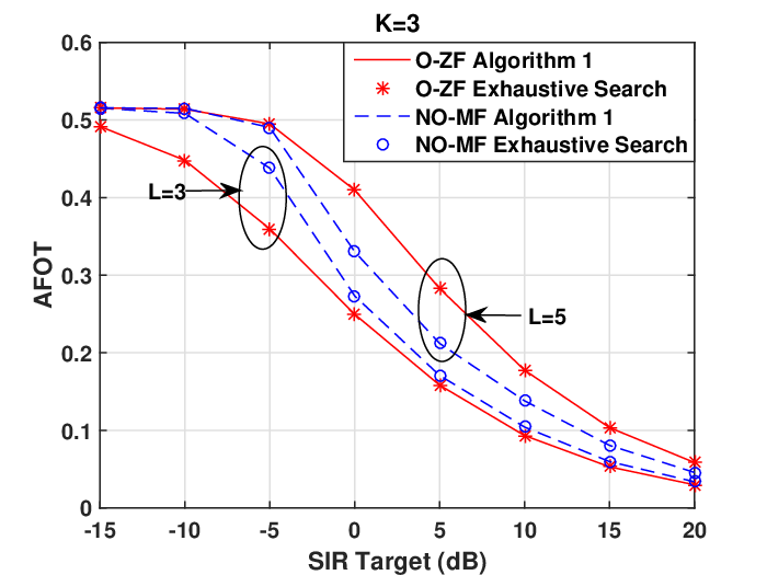
Fig. 6 illustrates the AESE of OPC and MPC for different number of antennas. It is observed that OPC outperforms MPC in both MF and ZF while the performance gap between OPC and MPC when ZF is applied is larger than that when MF is applied. This is because users suffer strong interference in MF, which causes that the AESE is mainly limited by the performance of the nearest SBS. Besides, the performance gain of OPC over MPC becomes larger by increasing the number of antennas. As such, we can conclude that OPC benefits better from multiple antennas than MPC.
For different beamforming types, Fig. 6 shows that ZF outperforms MF when . The reasons are similar to the AFOT case.
VI-C Comparison between MF and ZF for coded caching
Since Algorithm 1 is a greedy algorithm, we first validate its effectiveness. For illustration purpose, we only consider the AFOT maximization problem for validation. Fig. 6 shows that the results obtained by Algorithm 1 are almost identical to the optimal solution obtained by exhaustive search. Therefore, we can utilize Algorithm 1 to obtain the coded caching solution.
VI-C1 AFOT
Fig. 8 illustrates the AFOT of CC and MPC for different antenna number. At low SIR target ( dB), CC has a great performance gain over MPC since it can make a better utilization of collaborative caching among multiple SBSs. However, at high SIR target ( dB), CC outperforms MPC slightly with ZF and it even performs the same as MPC with MF. This is because users have a large probability to only connect to the nearest SBS when the decoding threshold is very stringent, and hence the performance of MPC is close to that of CC. Besides, AFOT for both O-ZF and NO-MF increase as grows, but the gain is diminishing. Moreover, the performance gap between CC and MPC also becomes larger by increasing , which means CC can enjoy a higher performance gain from multiple antennas than MPC.
Fig. 8 shows that NO-MF outperforms O-ZF at low SIR target. This is because in NO-MF, the effective channel gain of the desired signal is larger than O-ZF and the strong interference from closer SBSs is canceled simultaneously via SIC-based receiver. When the SIR target is high, users have a large probability to only be served by the nearest SBS. Therefore, O-ZF performs better than NO-MF when , which is similar to the probabilistic caching case.
VI-C2 AESE
Fig. 8 illustrates the AESE of CC and MPC for different number of antennas. It is observed that when MF beamforming is applied, CC performs almost the same as MPC for all ’s. This is because the AESE is limited by the minimum delivery rate of the serving SBSs in the concurrent transmission, and thus users prefer only connecting to the nearest SBS. When ZF beamforming is applied, on the other hand, CC outperforms MPC since it can make a better utilization of multiple SBSs. Moreover, ZF outperforms MF in coded caching. As such, in contrast to the previous finding in [24] where CC performs nearly to MPC in terms of AESE in the single-antenna system, we find that CC outperforms considerably MPC in the multi-antenna case if proper beamforming is chosen.


VI-D Impact of Imperfect CSI


Fig. 10 and Fig. 10 show that imperfect CSI degrades the performance of caching in both ZF and MF. Comparing ZF and MF, it is observed MF is more robust than ZF with imperfect CSI since each SBS needs to know more CSI to do the coordination when ZF is applied. Besides, the performance comparison between ZF and MF for differen with imperfect CSI is similar to the perfect CSI case. Moreover, when the number of feedback bits increases, the performance of imperfect CSI gets closer to that of perfect CSI case.
VII Conclusion
In this work, we analyze and optimize the probabilistic caching and coded caching in cache-enabled multi-antenna SCNs. We propose a user-centric SBS clustering and transmission framework, which allows each user to connect with the nearest SBSs within its cluster. We obtain approximate and compact integral expressions of AFOT and AESE, respectively, with MF and ZF beamforming. Then we formulate the cache placement problem to find the optimal cache solutions. The probabilistic cache placement problem is shown to be convex and optimal solutions are obtained. The coded cache placement problem is a MCKP and we solve it with a greedy-based low-complexity algorithm efficiently. We also extend the analysis and optimization above to the imperfect case. Numerical results show that multiple antennas can boost the advantage of probabilistic caching and coded caching over the traditional most popular caching with the proper use of beamforming. Numerical results also demonstrate the performance difference between MF and ZF under different number of antennas in both perfect and imperfect CSI cases.
Appendix A: Proof of Lemma 1
The coverage probability can be written as:
| (57) |
where (a) follows from the series expansion of the CCDF for Gamma distribution when is a positive integer, i.e., ; and (b) follows from the derivative property of the Laplace transform: .
The interference consists of two parts, the interference from the SBSs closer to than the serving SBS and the interference from the SBSs farther than . The Laplace transform of is given by:
| (58) |
where (a) follows from i.i.d. exponential distribution with unit mean of and it is also independent with the HPPP . Step (b) follows from that the locations of SBSs are independently and uniformly distributed in the circle area . The Laplace transform of is given by:
| (59) |
where the last step follows from the probability generating functional (PGFL) of the HPPP. Thus, Lemma 1 is proved.
Appendix B: Proof of Theorem 1
From the Alzer’s Inequality [42, 41], the the coverage probability is upper bounded as:
| (60) |
To simplify (60), we first rewrite the Laplace transform of the interference as:
| (61) |
where the last step follows by first replacing with , then replacing with . Therefore, the Laplace transform in (60) can be written as:
| (62) |
where and are defined for notation simplicity, given by (14) and (15), respectively, with . Next we need to calculate the expectation of over from (60). It is observed that only the inter-cluster interference is related to . Therefore, evaluating the expectation of is enough, which is given by:
| (63) |
where step (a) follows from the change of variable and step (b) follows from the Gamma distribution property that .
By substituting (63) into (60), we obtain the upper bound of the coverage probability (12). The lower bound (13) can be similarly proved by letting in the above derivations. This theorem is thus proved.
Appendix C: Proof of Theorem 2
Similar to the proof of Theorem , the coverage probability in ZF can be upper bounded by:
| (64) |
By substituting for in (59), we obtain the Laplace transform of inter-cluster interference, which is given by:
| (65) |
By introducing a parameter , the Laplace transform in (64) can be written as:
| (66) |
where the last step follows from the change of variable . For notation simplicity, we let
| (67) |
From (66), it is observed that we need to calculate the expectation over and , rather than and as in (64). Thus, we first calculate the expectation of (66) over .
| (68) |
where the last step follows from the change of variables similar to (63). Therefore, is given by:
| (69) |
To obtain the expectation above over , we first need to know the pdf of . Utilizing the joint pdf of and given in (18), the CDF of is given by:
| (70) |
where . Then, the pdf of can be obtained as:
| (71) |
Recall (67), we approximate the integral in it as a constant value according to randomness of . By utilizing partial integration, we can calculate that . Therefore, we approximate the integral in (67) as a constant value according to randomness of similar to [33, Eqn. (28)] as:
| (72) |
Thus, we can approximate as . Therefore, we have
| (73) |
Substituting (73) into (69), we obtain the approximate upper bound of the coverage probability (20). The approximate lower bound (21) can be similarly proved by letting in the above derivations. This theorem is thus proved.
Appendix D: Proof of Lemma 3
To prove the convexity of P1, we first prove that the coverage probabilities in both MF and ZF schemes are non-increasing functions of . For the exact coverage probabilities, this property holds obviously. For the lower bound (13) for MF, we have
| (74) |
where the last step follows from that and since all are i.i.d. random variables. Therefore, we conclude that the approximate probability in MF scheme is a non-increasing function of . For the ZF scheme, the proof is similar to the MF scheme.
Since the coverage probabilities in both MF and ZF schemes are non-increasing functions of , the second order derivative of the objective function (23) respect to can be expressed as:
| (75) |
where the previous steps come from the property that is non-increasing of and the last step follows from that . Since objective of P1 is to maximize a concave function and all constraints are linear, P1 is a convex problem in terms of AFOT maximization.
Since is also a non-increasing function of , the objective function AESE can be proved to be concave similar to AFOT above. Therefore, the proof is completed.
Appendix E: Proof of Theorem 3
For AFOT maximization, the Lagrangian function of P1 can be written as:
| (76) |
where is the Lagrangian multiplier associated with the constraint (27). By letting the partial derivative of the Lagrangian function to be , we have
| (77) |
It is easy to find that the left hand of (77) is a decreasing function of since the objective function is concave. Notice that we have the constraint . Thus, when , has the minimum value: . While for , it has the maximum value: . Therefore, the cache solution is given by:
| (78) |
which is equivalent to (28) by substituting for in (78). Hence, the proof is completed.
For AESE maximization, the proof is similar and hence is omitted here.
References
- [1] X. Xu and M. Tao, “Analysis and optimization of probabilistic caching in multi-antenna small-cell networks,” in IEEE Proc. Global Commun. Conf. (GLOBECOM), Dec. 2017, pp. 1–6.
- [2] E. Bastug, M. Bennis, and M. Debbah, “Living on the edge: The role of proactive caching in 5g wireless networks,” IEEE Commun. Mag., vol. 52, no. 8, pp. 82–89, Aug. 2014.
- [3] K. Shanmugam, N. Golrezaei, A. G. Dimakis, A. F. Molisch, and G. Caire, “Femtocaching: Wireless content delivery through distributed caching helpers,” IEEE Trans. Inf. Theory, vol. 59, no. 12, pp. 8402–8413, Dec. 2013.
- [4] X. Wang, M. Chen, T. Taleb, A. Ksentini, and V. C. Leung, “Cache in the air: exploiting content caching and delivery techniques for 5g systems,” IEEE Commun. Mag., vol. 52, no. 2, pp. 131–139, Feb. 2014.
- [5] N. Golrezaei, A. F. Molisch, A. G. Dimakis, and G. Caire, “Femtocaching and device-to-device collaboration: A new architecture for wireless video distribution,” IEEE Commun. Mag., vol. 51, no. 4, pp. 142–149, Apr. 2013.
- [6] G. Barish and K. Obraczke, “World wide web caching: Trends and techniques,” IEEE Commun. mag., vol. 38, no. 5, pp. 178–184, May. 2000.
- [7] A. Khreishah, J. Chakareski, and A. Gharaibeh, “Joint caching, routing, and channel assignment for collaborative small-cell cellular networks,” IEEE J. Sel. Areas Commun., vol. 34, no. 8, pp. 2275–2284, Aug. 2016.
- [8] G. Paschos, E. Bastug, I. Land, G. Caire, and M. Debbah, “Wireless caching: technical misconceptions and business barriers,” IEEE Commun. Mag., vol. 54, no. 8, pp. 16–22, Aug. 2016.
- [9] E. Bastug, M. Bennis, M. Kountouris, and M. Debbah, “Cache-enabled small cell networks: Modeling and tradeoffs,” EURASIP J. on Wireless Commun. and Netw., vol. 2015, no. 1, pp. 1–11, Feb. 2015.
- [10] C. Yang, Y. Yao, Z. Chen, and B. Xia, “Analysis on cache-enabled wireless heterogeneous networks,” IEEE Trans. Wireless Commun, vol. 15, no. 1, pp. 131–145, Jan. 2016.
- [11] X. Peng, J.-C. Shen, J. Zhang, and K. B. Letaief, “Backhaul-aware caching placement for wireless networks,” in IEEE Proc.Global Commun. Conf. (GLOBECOM), Dec. 2015, pp. 1–6.
- [12] B. Blaszczyszyn and A. Giovanidis, “Optimal geographic caching in cellular networks,” in IEEE Proc. Int. Conf. Commun (ICC), Jun. 2015, pp. 3358–3363.
- [13] S. H. Chae and W. Choi, “Caching placement in stochastic wireless caching helper networks: Channel selection diversity via caching,” IEEE Trans. Wireless Commun., vol. 15, no. 10, pp. 6626–6637, Oct. 2016.
- [14] Y. Cui and D. Jiang, “Analysis and optimization of caching and multicasting in large-scale cache-enabled heterogeneous wireless networks,” IEEE Trans. Wireless Commun, vol. 16, no. 1, pp. 250–264, Jan. 2017.
- [15] Y. Chen, M. Ding, J. Li, Z. Lin, G. Mao, and L. Hanzo, “Probabilistic small-cell caching: Performance analysis and optimization,” IEEE Trans. Veh. Technol., vol. 66, no. 5, pp. 4341–4354, May. 2017.
- [16] J. Li, W. Chen, M. Xiao, F. Shu, and X. Liu, “Efficient video pricing and caching in heterogeneous networks,” IEEE Trans. Veh. Techno., vol. 65, no. 10, pp. 8744–8751, Oct. 2016.
- [17] S. T. ul Hassan, M. Bennis, P. H. J. Nardelli, and M. Latva-aho, “Caching in wireless small cell networks: A storage-bandwidth tradeoff,” IEEE Commun. Lett., vol. 20, no. 6, pp. 1175–1178, Jun. 2016.
- [18] B. Bharath, K. Nagananda, and H. V. Poor, “A learning-based approach to caching in heterogenous small cell networks,” IEEE Trans. Commun., vol. 64, no. 4, pp. 1674–1686, Apr. 2016.
- [19] K. Li, C. Yang, Z. Chen, and M. Tao, “Optimization and analysis of probabilistic caching in -tier heterogeneous networks,” IEEE Trans. Wireless Commun., vol. 17, no. 2, pp. 1283–1297, Feb. 2018.
- [20] V. Bioglio, F. Gabry, and I. Land, “Optimizing MDS codes for caching at the edge,” in IEEE Proc. Global Commun. Conf. (GLOBECOM), Dec. 2015, pp. 1–6.
- [21] J. Liao, K. K. Wong, M. R. A. Khandaker, and Z. Zheng, “Optimizing cache placement for heterogeneous small cell networks,” IEEE Commun. Lett., vol. 21, no. 1, pp. 120–123, Jan. 2017.
- [22] E. Altman, K. Avrachenkov, and J. Goseling, “Coding for caches in the plane,” arXiv preprint arXiv:1309.0604, 2013.
- [23] Z. Chen, J. Lee, T. Q. S. Quek, and M. Kountouris, “Cooperative caching and transmission design in cluster-centric small cell networks,” IEEE Trans. Wireless Commun., vol. 16, no. 5, pp. 3401–3415, May. 2017.
- [24] X. Xu and M. Tao, “Modeling, analysis, and optimization of coded caching in small-cell networks,” IEEE Trans. Commun., vol. 65, no. 8, pp. 3415–3428, Aug. 2017.
- [25] A. Tang, S. Roy, and X. Wang, “Coded caching for wireless backhaul networks with unequal link rates,” IEEE Trans. Commun., vol. 66, no. 1, pp. 1–13, Jan. 2018.
- [26] X. Peng, J. C. Shen, J. Zhang, and K. B. Letaief, “Joint data assignment and beamforming for backhaul limited caching networks,” in IEEE Proc. Int. Symp. Pers., Indoor, Mobile Radio Commun. (PIMRC), Sep. 2014, pp. 1370–1374.
- [27] M. Tao, E. Chen, H. Zhou, and W. Yu, “Content-centric sparse multicast beamforming for cache-enabled cloud ran,” IEEE Trans. Wireless Commun., vol. 15, no. 9, pp. 6118–6131, Sep. 2016.
- [28] Y. Cao, M. Tao, F. Xu, and K. Liu, “Fundamental storage-latency tradeoff in cache-aided mimo interference networks,” IEEE Trans. Wireless Commun., vol. 16, no. 8, pp. 5061–5076, Aug. 2017.
- [29] Y. Cao and M. Tao, “Treating content delivery in multi-antenna coded caching as general message sets transmission: A dof region perspective,” arXiv preprint arXiv:1807.01432, 2018.
- [30] D. Liu and C. Yang, “Caching policy toward maximal success probability and area spectral efficiency of cache-enabled HetNets,” IEEE Trans. Commun., vol. 65, no. 6, pp. 2699–2714, Jun. 2017.
- [31] N. Jindal, J. G. Andrews, and S. Weber, “Multi-antenna communication in ad hoc networks: Achieving MIMO gains with SIMO transmission,” IEEE Trans. Commun., vol. 59, no. 2, pp. 529–540, Feb. 2011.
- [32] C. Li, J. Zhang, M. Haenggi, and K. B. Letaief, “User-centric intercell interference nulling for downlink small cell networks,” IEEE Trans. Commun., vol. 63, no. 4, pp. 1419–1431, Apr. 2015.
- [33] N. Lee, D. Morales-Jimenez, A. Lozano, and R. W. Heath, “Spectral efficiency of dynamic coordinated beamforming: A stochastic geometry approach,” IEEE Trans. Wireless Commun., vol. 14, no. 1, pp. 230–241, Jan. 2015.
- [34] J. G. Andrews, F. Baccelli, and R. K. Ganti, “A tractable approach to coverage and rate in cellular networks,” IEEE Trans. Commun., vol. 59, no. 11, pp. 3122–3134, Nov. 2011.
- [35] M. A. Maddah-Ali and U. Niesen, “Fundamental limits of caching,” IEEE Trans. Inf. Theory, vol. 60, no. 5, pp. 2856–2867, May. 2014.
- [36] S. T. Veetil, K. Kuchi, and R. K. Ganti, “Performance of pzf and mmse receivers in cellular networks with multi-user spatial multiplexing,” IEEE Trans. Wireless Commun., vol. 14, no. 9, pp. 4867–4878, Sep. 2015.
- [37] M. Haenggi, “On distances in uniformly random networks,” IEEE Trans. Inf. Theory, vol. 51, no. 10, pp. 3584–3586, Oct. 2005.
- [38] S. Srinivasa and M. Haenggi, “Distance distributions in finite uniformly random networks: Theory and applications,” IEEE Trans. Veh. Technol., vol. 59, no. 2, pp. 940–949, Feb. 2010.
- [39] M. Wildemeersch, T. Q. Quek, M. Kountouris, A. Rabbachin, and C. H. Slump, “Successive interference cancellation in heterogeneous networks,” IEEE Trans. Commun., vol. 62, no. 12, pp. 4440–4453, Dec. 2014.
- [40] D. J. Love, R. W. Heath, V. K. N. Lau, D. Gesbert, B. D. Rao, and M. Andrews, “An overview of limited feedback in wireless communication systems,” IEEE J. Sel. Areas Commun., vol. 26, no. 8, pp. 1341–1365, Oct. 2008.
- [41] H. Alzer, “On some inequalities for the incomplete gamma function,” Math. Comput., vol. 66, no. 218, pp. 771–778, Apr. 1997.
- [42] K. Huang, R. W. Heath, and J. G. Andrews, “Space division multiple access with a sum feedback rate constraint,” IEEE Trans. Signal Processing, vol. 55, no. 7, pp. 3879–3891, Jul. 2007.