跳到论文正文
W Papers独立论文阅读器 arXiv:1908.06485 论文正文 计算阅读时间 · 0%
引用这篇论文根据当前论文元数据生成,正式投稿前建议核对。


License: arXiv.org perpetual non-exclusive license
arXiv:1908.06485v1 [math.AP] 18 Aug 2019

The selection problem for some first-order stationary Mean-field gamesThanks:  D. Gomes was partially supported by King Abdullah University of Science and Technology (KAUST) baseline funds and KAUST OSR-CRG2017-3452. H. Mitake was partially supported by the JSPS grants: KAKENHI #19K03580, #19H00639, #16H03948, #17KK0093. K. Terai was supported by King Abdullah University of Science and Technology (KAUST) through the Visiting Student Research Program (VSRP)

Diogo A. Gomes D. A. Gomes King Abdullah University of Science and Technology (KAUST), CEMSE Division, Thuwal 23955-6900. Saudi Arabia, and KAUST SRI, Center for Uncertainty Quantification in Computational Science and Engineering. Email address: diogo.gomes@kaust.edu.sa , Hiroyoshi Mitake H. Mitake Graduate School of Mathematical Sciences, University of Tokyo, 3-8-1 Komaba, Meguro-ku, Tokyo, 153-8914, Japan. Email address: mitake@ms.u-tokyo.ac.jp and Kengo Terai K. Terai Graduate School of Mathematical Sciences, University of Tokyo, 3-8-1 Komaba, Meguro-ku, Tokyo, 153-8914, Japan. Email address: terai@ms.u-tokyo.ac.jp
Date: August 11, 2026
Abstract.

Here, we study the existence and the convergence of solutions for the vanishing discount MFG problem with a quadratic Hamiltonian. We give conditions under which the discounted problem has a unique classical solution and prove convergence of the vanishing-discount limit to a unique solution up to constants. Then, we establish refined asymptotics for the limit. When those conditions do not hold, the limit problem may not have a unique solution and its solutions may not be smooth, as we illustrate in an elementary example. Finally, we investigate the stability of regular weak solutions and address the selection problem. Using ideas from Aubry-Mather theory, we establish a selection criterion for the limit.

Key words and phrases: 
Mean field games; Hamilton-Jacobi equation; selection problem; vanishing discount
2010 Mathematics Subject Classification
35A01, 49L25, 91A13.

1. Introduction

Mean-field games (MFG) model systems with many rational noncooperative players, describe the player’s optimal strategies and determine the statistical properties of their distribution. These games are often determined by a system of a Hamilton-Jacobi equation coupled with a transport or Fokker-Planck equation. In the study of stationary Hamilton-Jacobi equations, a standard method to obtain a solution is to consider the vanishing discount problem. This was the strategy used originally in [31] in the study of homogenization problems. For second-order MFG, the existence of a solution for the discounted problem was shown, for example, in [20] and [8] and for first-order MFG in [16] in the sense of weak solutions and in [3] using variational methods. In the second-order case, the vanishing discount limit was studied in [4]. In the first-order case, the theory is not as much developed and the vanishing discount limit has not been examined previously. Here, our goal is to study the limit behavior as ϵ→0\epsilon\to 0 of the following discounted first-order stationary mean-field game.

Problem 1.

Let 𝕋d{\mathbb{T}}^{d} be the dd-dimensional flat torus identified with [0,1]d[0,1]^{d}. Let V:𝕋d→ℝV:{\mathbb{T}}^{d}\to{\mathbb{R}}, V∈C1,α​(𝕋d)V\in C^{1,\alpha}({\mathbb{T}}^{d}), g:[0,∞)→ℝ∪{−∞}g:[0,\infty)\to{\mathbb{R}}\cup\{-\infty\}, g∈C1,α​((,,,))g\in C^{1,\alpha}((0,+\infty)), with gg strictly increasing, and fix a discount rate, ϵ>0\epsilon>0. Find uϵ,mϵ:𝕋d→ℝu^{\epsilon},m^{\epsilon}:{\mathbb{T}}^{d}\to{\mathbb{R}} with mϵ​(x)⩾0m^{\epsilon}(x)\geqslant 0 such that

(1.1) {ϵ​uϵ+12​|D​uϵ|2+V⁡(x)=g⁡(mϵ)in​𝕋d,ϵ​mϵ−div⁡(mϵ​D​uϵ)=ϵin​𝕋d.\begin{cases}&\epsilon u^{\epsilon}+\frac{1}{2}|Du^{\epsilon}|^{2}+V(x)=g(m^{\epsilon})\quad\rm{in}\ {\mathbb{T}}^{d},\\ &\epsilon m^{\epsilon}-\mathrm{div}(m^{\epsilon}Du^{\epsilon})=\epsilon\quad\rm{in}\ {\mathbb{T}}^{d}.\\ \end{cases}

We say that (uϵ,mϵ)(u^{\epsilon},m^{\epsilon}) is a classical solution of the preceding problem if uϵ∈C2,α​(𝕋d)u^{\epsilon}\in C^{2,\alpha}({\mathbb{T}}^{d}) and mϵ∈C1,α​(𝕋d)m^{\epsilon}\in C^{1,\alpha}({\mathbb{T}}^{d}) with mϵ⩾0m^{\epsilon}\geqslant 0. As we show in Proposition 3.1, mϵm^{\epsilon} cannot vanish, hence, mϵ>0m^{\epsilon}>0. As in the case of Hamilton-Jacobi equations, we expect that, as ϵ→0\epsilon\to 0, the solutions of (1.1) converge, maybe through subsequences after adding a suitable constant to uϵu^{\epsilon}, to a solution of the following first-order MFG.

Problem 2.

With gg, VV as in Problem 1, find u,m:𝕋d→ℝu,m:{\mathbb{T}}^{d}\to{\mathbb{R}} with m⩾0m\geqslant 0 and H¯∈ℝ{\overline{H}}\in{\mathbb{R}} such that

(1.2) {12​|D​u|2+V⁡(x)=g⁡(m)+H¯in​𝕋d,−div⁡(m​D​u)=0in​𝕋d,m(x)⩾0,∫𝕋dmdx=1.\begin{cases}&\frac{1}{2}|Du|^{2}+V(x)=g(m)+\bar{H}\quad\text{in}\ {\mathbb{T}}^{d},\\ &-\mathrm{div}(mDu)=0\quad\text{in}\ {\mathbb{T}}^{d},\\ &m(x)\geqslant 0,\ \ \int_{{\mathbb{T}}^{d}}mdx=1.\end{cases}

Because (1.2) is invariant under addition of constants to uu, we can prescribe the additional normalization condition

(1.3) ∫𝕋du​𝑑x=0.\int_{{\mathbb{T}}^{d}}udx=0.

According to [16] (also see [17]), Problem 2 admits weak solutions under suitable polynomial growth conditions of gg, see Corollary 6.3 in [16]. Here, in Section 7, under a different set of hypothesis and using a limiting argument, we establish the existence of solutions for Problem 2. A natural question in the analysis of the limit ϵ→0\epsilon\to 0 is the selection problem; that is, whether the sequence (uϵ,mϵ)(u^{\epsilon},m^{\epsilon}) converges (not just whether a subsequence converges) and if so, what is the limit among all possible solutions of (1.2). This matter is our main focus here.

For Hamilton-Jacobi equations, the discounted problem corresponds to the following control problem. Let 𝐱⁡(t)∈ℝd{\bf x}(t)\in{\mathbb{R}}^{d} be the state of an agent at the time tt. This agent can change its state by choosing a control 𝐯∈L∞​([0,∞),ℝd){\bf v}\in L^{\infty}([0,\infty),{\mathbb{R}}^{d}). Thus, its trajectory, 𝐱⁡(𝐭)\bf{x}(t), is determined by 𝐱˙​(t)=𝐯​(t)\dot{\bf{x}}\rm(t)=\bf{v}\rm(t), with initial condition 𝐱⁡(t)=x∈𝕋d{\bf x}(t)=x\in{\mathbb{T}}^{d}. The agent selects the control to minimize the cost functional

J⁡(x,𝐯)=∫0∞e−ϵ​t​L​(𝐱⁡(t),𝐱˙​(t))​𝑑t,J(x;{\bf v})=\int^{\infty}_{0}e^{-\epsilon t}L({\bf x}(t),\dot{{\bf x}}(t))\,{\rm d}t,

for a given Lagrangian, L:𝕋d×ℝd→ℝL:{\mathbb{T}}^{d}\times{\mathbb{R}}^{d}\to{\mathbb{R}}. The value function, uϵu^{\epsilon}, is given by

uϵ​(x)=inf𝐯J⁡(x,𝐯),u^{\epsilon}(x)=\inf_{\bf{v}}J(x;{\bf v}),

where the infimum is taken over 𝐯∈L∞([0,+∞),ℝd){\bf v}\in L^{\infty}([0,+\infty),{\mathbb{R}}^{d}).

The Hamiltonian, H:𝕋d×ℝd→ℝH:{\mathbb{T}}^{d}\times{\mathbb{R}}^{d}\to{\mathbb{R}}, corresponding to this control problem is the Legendre transform of LL; that is,

H(x,p)=supv∈ℝd−p⋅v−L(x,v).H(x,p)=\sup_{v\in{\mathbb{R}}^{d}}-p\cdot v-L(x,v).

Under standard coercivity and convexity assumptions on LL, uϵu^{\epsilon} is the unique viscosity solution of the discounted Hamilton-Jacobi equation,

(1.4) ϵ​uϵ+H⁡(x,D​uϵ)=0in​𝕋d.\epsilon u^{\epsilon}+H(x,Du^{\epsilon})=0\quad\rm{in}\ {\mathbb{T}}^{d}.

For coercive Hamiltonians, the results in [31] give that ϵ​uϵ\epsilon u^{\epsilon} is uniformly bounded and that uϵu^{\epsilon} is equi-Lipschitz for ϵ>0\epsilon>0. Thus, uϵ−min𝕋d⁡uϵu^{\epsilon}-\min_{{\mathbb{T}}^{d}}u^{\epsilon} uniformly converges to a function, uu, along subsequences, as ϵ→0\epsilon\to 0. Moreover, ϵ​uϵ\epsilon u^{\epsilon} converges to a constant −H~-\tilde{H}. By stability of viscosity solutions, (u,H~)(u,\tilde{H}) solves the ergodic Hamilton-Jacobi equation

(1.5) H⁡(x,D​u)=H~in​𝕋d,H(x,Du)=\tilde{H}\quad\rm{in}\ {\mathbb{T}}^{d},

where the unknowns are u:𝕋d→ℝu:{\mathbb{T}}^{d}\to{\mathbb{R}} and H~∈ℝ\tilde{H}\in{\mathbb{R}}. However, the solution of (1.5) may not be unique. Hence, the solution constructed above could depend on the particular subsequence used to extract the limit. The study of the selection problem was started in [19] using the discounted Mather measures introduced in [2]. The main convergence result was established in [5]. Subsequently, several authors investigated and extended those ideas in [1], [26], [27], and [34] . Recently, the case of non-convex Hamiltonians was addressed in [21].

In MFGs, we consider a large population of agents where each agent seeks to optimize an objective function. Here, however, the running cost depends on statistical information about the players, encoded in a probability density, m:𝕋d×[0,∞)→ℝm:{\mathbb{T}}^{d}\times[0,\infty)\to{\mathbb{R}}. In the model discussed here, the Lagrangian is L^​(x,p)=12​|p|2−V⁡(x)+g⁡(m)\hat{L}(x,p)=\frac{1}{2}|p|^{2}-V(x)+g(m) and each agent seeks to minimize the functional

J^​(x)=∫0∞e−ϵ​t​[12​|𝐱˙​(t)|2−V⁡(𝐱⁡(t))+g⁡(m⁡(𝐱⁡(t),t))]​𝑑t.\hat{J}(x)=\int^{\infty}_{0}e^{-\epsilon t}\left[\frac{1}{2}|\dot{{\bf x}}(t)|^{2}-V({\bf x}(t))+g\big(m({\bf x}(t),t)\big)\right]\,{\rm d}t.

Now, we suppose that the value function, uϵ:=inf𝐯J,^u^{\epsilon}:=\inf_{{\bf v}}\hat{J,} is smooth. Then, uϵu^{\epsilon} solves the first equation in (1.1) and the optimal control is given by 𝐯⁡(t)=−D​uϵ​(𝐱⁡(t)){\bf v}(t)=-Du^{\epsilon}({\bf x}(t)). Because the players are rational, they use this optimal control. Here, ϵ\epsilon represents the rate at which players quit the game, which occurs at independent and memoryless times. Furthermore, new players join the game randomly at a rate ϵ\epsilon, as can be seen by looking at the right-hand side of the second equation in (1.1). Then, in the stationary configuration, the density, mm, is determined by the second equation in (1.1). Without an inflow of players, the only non-negative solution is trivial, m=0m=0.

The theory for second-order stationary MFG is now well developed and in many cases the existence of smooth solutions can be established, see for example [25], [24], [35], or [8]. For logarithmic nonlinearities, the existence of smooth solutions was proven in [9]. However, this is a special case; as shown in Section 2, for first-order MFG, the existence of smooth solutions may not hold (see also a detailed discussion in [23] and [22]). Thus, in general, we need to consider weak solutions, see [7] or [16] for an approach using monotone operators and [3] for a variational approach.

One of the difficulties of first-order stationary MFG is the lack of regularizing terms in both the Hamilton-Jacobi equation and in the transport equation. Nonetheless, the MFG system behaves somewhat like an elliptic equation. Here, we explore this effect and obtain conditions under which Problem 1 has classical solutions. These conditions are given in the following two assumptions.

Assumption 1.

gg and VV satisfy that g−1​(g⁡(1)−oscx∈𝕋d​V​(x))>0g^{-1}\big(g(1)-\mathrm{osc}_{x\in{\mathbb{T}}^{d}}V(x)\big)>0.

Assumption 2.

There exist constants C1>0C_{1}>0, C2>0C_{2}>0 and β∈ℝ\beta\in{\mathbb{R}} such that for all z⩾0z\geqslant 0,

g′​(z)⩾C1​zβ,g^{\prime}(z)\geqslant C_{1}z^{\beta},
g⁡(z)⩽C2+z​g​(z).g(z)\leqslant C_{2}+zg(z).

An example that satisfies the preceding assumptions is the following:

g⁡(m)=mα​(α>0),V⁡(x)=c​sin⁡(2​π​x)​(0<c<1/2),g(m)=m^{\alpha}\>\>(\alpha>0),\>\>V(x)=c\sin(2\pi x)\,\,(0<c<1/2),

where d=1d=1 and VV is extended by periodicity to ℝ{\mathbb{R}}. The preceding two assumptions are used to obtain lower bounds on the density and can be interpreted as follows. Because gg is increasing agents want to avoid crowded areas and prefer areas with low density. However, if the oscillation of the potential is large, the trade-off between a low-density area with high potential and a high-density area with low potential may not pay-off. Hence, the control of the oscillation of VV given in Assumption 1 implies that no point is totally avoided by the agents.

As we mentioned previously, the two preceding assumptions imply the existence of a classical solution for Problem 1 as stated in the following theorem.

Theorem 1.1.

Suppose that Assumptions 1 and 2 hold. Then, for each ϵ>0\epsilon>0, Problem 1 has a unique classical solution (uϵ,mϵ)(u^{\epsilon},m^{\epsilon}) with mϵ>0m^{\epsilon}>0.

The proof of this theorem is given in Section 5 using a continuation method combined with the a priori estimates in Section 3 and the DeGiorgi-Nash-Moser argument outlined in Section 4. As a corollary of the preceding theorem, we obtain our first convergence result.

Corollary 1.2.

Suppose that Assumptions 1 and 2 hold. Then, Problem 2 has a unique classical solution (u,m,H¯)(u,m,\bar{H}), with m>0m>0 and ∫𝕋du​𝑑x=0\int_{{\mathbb{T}}^{d}}udx=0. Furthermore, let (uϵ,mϵ)(u^{\epsilon},m^{\epsilon}) solve Problem 1. Then

uϵ−∫𝕋duϵ dx→uinC2,α(𝕋d),mϵ→minC1,α(𝕋d),ϵuϵ→−H¯uniformly. u^{\epsilon}-\int_{{\mathbb{T}}^{d}}u^{\epsilon}\mbox{ }dx\to u\>\>\>\text{in}\ C^{2,\alpha}({\mathbb{T}}^{d}),\quad m^{\epsilon}\to m\>\>\>\text{in}\ C^{1,\alpha}({\mathbb{T}}^{d}),\quad\epsilon u^{\epsilon}\to-{\overline{H}}\>\>\>\text{uniformly. }

The proof of this corollary is given at the end of Section 5.

For second-order MFGs, the vanishing discount problem for mean-field games was addressed in [4]. Inspired by the approach there, we consider the following formal asymptotic expansion

(1.6) uϵ−H¯/ϵ∼u+λ+ϵ​v,mϵ∼m+ϵ​θu^{\epsilon}-\bar{H}/\epsilon\sim u+\lambda+\epsilon v,\qquad m^{\epsilon}\sim m+\epsilon\theta

for the solution of Problem 1. Using this expansion in (1.1), assuming that (u,m,λ)(u,m,\lambda) solves Problem 2, and matching powers of ϵ\epsilon, we obtain the following problem that determines the terms λ\lambda, vv, and θ\theta in (1.6). To simplify the presentation, we discuss the case of C∞C^{\infty}- solutions.

Problem 3.

Let gg be as in Problem 1 with g∈C∞g\in C^{\infty} and let (u,m)(u,m) be C∞C^{\infty}- solutions of Problem 2 with m>0m>0 and ∫u=0\int u=0. Find v,θ:𝕋d→ℝv,\theta:{\mathbb{T}}^{d}\to{\mathbb{R}} and λ∈ℝ\lambda\in{\mathbb{R}} such that

(1.7) {λ+u+D​u⋅D​v=g′​(m)​θin​𝕋d,−div⁡(m​D​v)−div⁡(θ​D​u)=1−min​𝕋d.\begin{cases}&\lambda+u+Du\cdot Dv=g^{\prime}(m)\theta\quad\rm{in}\ {\mathbb{T}}^{d},\\ &-\mathrm{div}(mDv)-\mathrm{div}(\theta Du)=1-m\quad\rm{in}\ {\mathbb{T}}^{d}.\end{cases}
Remark 1.3.

The normalization condition ∫u​𝑑x=0\int udx=0 is required for the uniqueness of the constant λ\lambda. Given a solution of (1.7), by adding a constant κ\kappa to uu and subtracting κ\kappa to λ\lambda, we produce another solution.

The existence of a solution to the preceding problem is established in Proposition 6.5 in Section 6. In that section, we prove the following improved asymptotic rate of convergence.

Theorem 1.4.

Suppose Assumption 2 holds. Let (uϵ,mϵ)(u^{\epsilon},m^{\epsilon}) and (u,m,H¯)(u,m,\bar{H}), with m>0m>0 and ∫u=0\int u=0, be classical solutions of, respectively, Problems 1 and 2. Let (v,θ,λ)(v,\theta,\lambda) be the corresponding classical solution to Problem 3. Then,

limϵ→0‖uϵ−H¯ϵ−u−λ‖∞+‖mϵ−m‖∞=0.\lim_{\epsilon\to 0}\left\|u^{\epsilon}-\frac{\bar{H}}{\epsilon}-u-\lambda\right\|_{\infty}+\|m^{\epsilon}-m\|_{\infty}=0.
Remark 1.5.

The preceding theorem remains valid if we replace Assumption 2 with the weaker condition that for any z0>0z_{0}>0 there exists γ⁡(z0)>0\gamma(z_{0})>0 such that

g′​(z)>γ⁡(z0)g^{\prime}(z)>\gamma(z_{0})

for all z>z0z>z_{0}.

In the last section of the paper, Section 7, we investigate the asymptotic behavior of (uϵ,mϵ)(u^{\epsilon},m^{\epsilon}) as ϵ→0\epsilon\to 0. Here, we work with weak solutions in the sense of the definition below, and we consider the case where uniqueness of solution for Problem 2 may not hold. In this case, we replace Assumption 1 and 2 the following assumption that still allows the existence of solutions to be established.

Assumption 3.

There exist positive constants, c1,c2⩾0c_{1},c_{2}\geqslant 0, and a positive real number, α\alpha, with

  • -

    α>0\alpha>0 if d⩽4d\leqslant 4

  • -

    α>d−4d\alpha>\frac{d-4}{d} if 4<d⩽84<d\leqslant 8

  • -

    α>d−42\alpha>\frac{d-4}{2} if d⩾8d\geqslant 8

such that

c1​mα−1⩽g′​(m)⩽c2​mα−1c_{1}m^{\alpha-1}\leqslant g^{\prime}(m)\leqslant c_{2}m^{\alpha-1}

for all m>0m>0.

Remark 1.6.

From the preceding hypothesis, we obtain that there exist positive constants c~1,c~2\tilde{c}_{1},\tilde{c}_{2} and CC such that

c~1​mα−C⩽g⁡(m)⩽c~2​mα+C.\tilde{c}_{1}m^{\alpha}-C\leqslant g(m)\leqslant\tilde{c}_{2}m^{\alpha}+C.

Of course, if Assumption 1 does not hold, we cannot ensure the existence of smooth solutions to Problem 1. Nonetheless, the existence of weak solutions for Problem 1 was proven in [16]. More precisely, we consider the following result.

Theorem 1.7 (from [16]).

Suppose that Assumption 3 holds. Then, Problem 1 has a weak solution (mϵ,uϵ)(m^{\epsilon},u^{\epsilon}) as follows. There exists a constant CC, independent of ϵ\epsilon such that

  1. 1.

    mϵ⩾0m^{\epsilon}\geqslant 0 and ∫𝕋dmϵ​𝑑x=1\int_{{\mathbb{T}}^{d}}m^{\epsilon}dx=1,

  2. 2.

    ‖(mϵ)α+12‖W1,2​(𝕋d)⩽C\|(m^{\epsilon})^{\frac{\alpha+1}{2}}\|_{W^{1,2}({\mathbb{T}}^{d})}\leqslant C,

  3. 3.

    ‖uϵ−∫𝕋duϵ​𝑑x‖W1,2​(𝕋d)⩽C\|u^{\epsilon}-\int_{{\mathbb{T}}^{d}}u^{\epsilon}dx\|_{W^{1,2}({\mathbb{T}}^{d})}\leqslant C,

  4. 4.

    |ϵ​∫𝕋duϵ​𝑑x|⩽C\left|\epsilon\int_{{\mathbb{T}}^{d}}u^{\epsilon}dx\right|\leqslant C,

  5. 5.

    ‖(mϵ)α+12​D​uϵ‖B​V​(𝕋d)⩽C\|(m^{\epsilon})^{\frac{\alpha+1}{2}}Du^{\epsilon}\|_{BV({\mathbb{T}}^{d})}\leqslant C.

Moreover,

(1.8) −ϵ​uϵ−|D​uϵ|22−V⁡(x)+g⁡(mϵ)⩾0-\epsilon u^{\epsilon}-\frac{|Du^{\epsilon}|^{2}}{2}-V(x)+g(m^{\epsilon})\geqslant 0

in the sense of distributions, with

(1.9) (−ϵ​uϵ−|D​uϵ|22−V⁡(x)+g⁡(mϵ))​mϵ=0,(-\epsilon u^{\epsilon}-\frac{|Du^{\epsilon}|^{2}}{2}-V(x)+g(m^{\epsilon}))m^{\epsilon}=0,

almost everywhere. Furthermore,

(1.10) ϵ​mϵ−div⁡(mϵ​D​uϵ)=ϵ,\epsilon m^{\epsilon}-\operatorname{div}(m^{\epsilon}Du^{\epsilon})=\epsilon,

in the sense of distributions and almost everywhere.

Similar techniques applied to Problem 2 yield the existence of a number H¯{\overline{H}} and functions (m,u)(m,u) satisfying estimates 1-3 and 5 in Theorem 1.7 such that

(1.11) H¯−|D​u|22−V⁡(x)+g⁡(m)⩾0{\overline{H}}-\frac{|Du|^{2}}{2}-V(x)+g(m)\geqslant 0

in the sense of distributions, with

(1.12) (H¯−|D​u|22−V⁡(x)+g⁡(m))​m=0,({\overline{H}}-\frac{|Du|^{2}}{2}-V(x)+g(m))m=0,

almost everywhere. Furthermore,

(1.13) −div⁡(m​D​u)=0,-\operatorname{div}(mDu)=0,

in the sense of distributions and almost everywhere.

When classical solutions are not available, we need to work with regular weak solutions, as defined next.

Definition 1.8.

A pair (mϵ,uϵ)(m^{\epsilon},u^{\epsilon}) is a regular weak solution of Problem 1 if it satisfies (1.8), (1.9) and (1.10) in the preceding theorem and, in particular, the same estimates 1-5 with the same constants. Similarly, a triple (u,m,H¯)(u,m,{\overline{H}}) is a regular weak solution of Problem 2 if it satisfies (1.11), (1.12), (1.13) and the estimates 1-5 in the preceding theorem with the same constants.

In Section 7, Proposition 7.1, we consider a sequence of regular weak solution of Problem 1 and show that, by extracting a subsequence if necessary, it converges to a regular weak solution of Problem 2. In particular, this approach gives the existence a regular weak solution for Problem 2.

Our selection result for regular weak solutions, proven in Section 7, is the following theorem.

Theorem 1.9.

Let (uϵ,mϵ)(u^{\epsilon},m^{\epsilon}) be a regular weak solution of Problem 1. Suppose that ⟨uϵ⟩⇀u¯\langle u^{\epsilon}\rangle\rightharpoonup\bar{u} in H1​(𝕋d)H^{1}({\mathbb{T}}^{d}) and that mϵ⇀m¯m^{\epsilon}\rightharpoonup\bar{m} weakly in L1​(𝕋d)L^{1}({\mathbb{T}}^{d}). Let (u,m)(u,m) be a regular weak solution of Problem 2. Then,

(1.14) ∫𝕋d(g⁡(mϵ)−g⁡(m))​(mϵ−m)​𝑑x→0\int_{{\mathbb{T}}^{d}}(g(m^{\epsilon})-g(m))(m^{\epsilon}-m)dx\to 0

and m¯=m\bar{m}=m. Moreover, we have

(1.15) ∫𝕋d⟨u¯⟩​m​𝑑x⩽∫𝕋d⟨u⟩​m​𝑑x,\int_{{\mathbb{T}}^{d}}\langle\bar{u}\rangle mdx\leqslant\int_{{\mathbb{T}}^{d}}\langle u\rangle mdx,

where

⟨f⟩=f⁡(x)−∫𝕋df​𝑑x.\langle f\rangle=f(x)-\int_{{\mathbb{T}}^{d}}fdx.

The proof of the preceding theorem relies on ideas from Aubry-Mather theory introduced in [19]. The paper ends with a short example that illustrates the preceding result.

2. Lack of uniqueness

Here, we examine the uniqueness of solutions of (1.2). First, we use the uniqueness method by Lasry-Lions [29] to show that the probability density, mm, is unique. Thus, failure of uniqueness for (1.2) requires multiplicity of solutions, uu, of the Hamilton-Jacobi equation. Second, we revisit an example from [23], where uniqueness does not hold. This example serves to illustrate the selection principle derived in Section 7.

2.1. Lasry-Lions method

The monotonicity argument introduced by Lasry-Lions (see, [28] or the lectures [30]), can be used to prove the uniqueness of solution for MFGs in the time-dependent case and gives the uniqueness of mm in the stationary problem. Here, we apply this technique to Problem 2. Let (u1,m2,H¯1)(u_{1},m_{2},\bar{H}_{1}) and (u2,m2,H¯2)(u_{2},m_{2},\bar{H}_{2}) be classical solutions of (1.2). Then,

{12​|D​u1|2−12​|D​u2|2+H¯1−H¯2=g⁡(m1)−g⁡(m2)−div⁡(m1​D​u1)+div⁡(m2​D​u2)=0.\begin{cases}&\frac{1}{2}|Du_{1}|^{2}-\frac{1}{2}|Du_{2}|^{2}+\bar{H}_{1}-\bar{H}_{2}=g(m_{1})-g(m_{2})\\ &-\mathrm{div}(m_{1}Du_{1})+\mathrm{div}(m_{2}Du_{2})=0.\\ \end{cases}

Now, we multiply the first equation by (m1−m2)(m_{1}-m_{2}) and the second equation by (u1−u2)(u_{1}-u_{2}). Next, subtracting the resulting identities and integrating by parts, we obtain

(2.1) ∫𝕋d(m1−m2)​(g⁡(m1)−g⁡(m2))+12​(m1+m2)​|D​u1−D​u2|2​𝑑x=0.\int_{{\mathbb{T}}^{d}}(m_{1}-m_{2})(g(m_{1})-g(m_{2}))+\frac{1}{2}(m_{1}+m_{2})|Du_{1}-Du_{2}|^{2}\,{\rm d}x=0.

Accordingly, m1=m2=mm_{1}=m_{2}=m on 𝕋d{\mathbb{T}}^{d} because gg is strictly increasing. Moreover, D​u1=D​u2Du_{1}=Du_{2} on m>0m>0. Hence, classical solutions (u,m,H¯)(u,m,\bar{H}) of (1.2) with m>0m>0 are unique up to an additive term in uu. Uniqueness may fail if mm vanishes, as we show in Section 2.2. A similar proof gives that (2.1) holds for the solutions of (1.1). By Lemma 3.1, mϵm^{\epsilon} is positive. Hence, classical solutions of Problem 1 are unique.

2.2. An explicit example

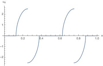
Here, we compute two distinct solutions of (1.2). In the example below, the existence of a unique smooth solutions fails and mm vanishes at an interval. We show that uu is a Lipschitz viscosity solution and mm is a probability density. These solutions are regular weak solutions as defined in Section 7.1.

Let g⁡(m)=mg(m)=m, d=1,d=1, and V⁡(x)=π​cos⁡(4​π​x)V(x)=\pi\cos(4\pi x). Then, (1.2) becomes

(2.2) {12​|ux|2+π​cos⁡(4​π​x)=m+H¯in​𝕋,−(m​ux)x=0in​𝕋,m(x)⩾0,∫m=1.\begin{cases}&\frac{1}{2}|u_{x}|^{2}+\pi\cos(4\pi x)=m+\bar{H}\quad\rm{in}\ {\mathbb{T}},\\ &-(mu_{x})_{x}=0\quad\rm{in}\ {\mathbb{T}},\\ &m(x)\geqslant 0,\ \ \int m=1.\end{cases}

From the second equation in (2.2), m​uxmu_{x} is constant. In particular, due to periodicity uu achieves a maximum or a minimum in 𝕋{\mathbb{T}}. At this maximum or minimum point ux=0u_{x}=0. Accordingly, m​ux=0mu_{x}=0. Thus, uu is constant on the set m>0m>0. From the first equation in (2.2) and taking into account that ∫𝕋m​𝑑x=1\int_{{\mathbb{T}}}mdx=1, we have H¯=0\bar{H}=0 and, thus,

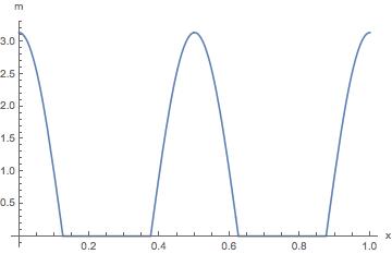
m⁡(x)=(π​cos⁡(4​π​x))+.m(x)=(\pi\cos(4\pi x))^{+}.

The preceding expression vanishes in an interval, as can be seen in Figure 1. Set

(u^​(x))x=\displaystyle(\hat{u}(x))_{x}= 2​(−π​cos⁡(4​π​x))+⋅χ{18<x<14∨58<x<34}\displaystyle\sqrt{2(-\pi\cos(4\pi x))^{+}}\cdot\chi_{\{\frac{1}{8}<x<\frac{1}{4}\vee\frac{5}{8}<x<\frac{3}{4}\}}
−2​(−π​cos⁡(4​π​x))+⋅χ{14<x<38∨34<x<78},\displaystyle-\sqrt{2(-\pi\cos(4\pi x))^{+}}\cdot\chi_{\{\frac{1}{4}<x<\frac{3}{8}\vee\frac{3}{4}<x<\frac{7}{8}\}},

and

(u~(x))x=2​(−π​cos⁡(4​π​x))+⋅χ{18<x<38}−2​(−π​cos⁡(4​π​x))+⋅χ{58<x<78},(\tilde{u}(x))_{x}=\sqrt{2(-\pi\cos(4\pi x))^{+}}\cdot\chi_{\{\frac{1}{8}<x<\frac{3}{8}\}}-\sqrt{2(-\pi\cos(4\pi x))^{+}}\cdot\chi_{\{\frac{5}{8}<x<\frac{7}{8}\}},

where χ\chi is the characteristic function. We observe that (u^,m,0)(\hat{u},m,0) and (u~,m,0)(\tilde{u},m,0) solve (2.2). These two solutions are viscosity solutions - u~x\tilde{u}_{x} is continuous, and uxu_{x} only has downward jumps, see Figures 2(a) and 2(b).
Refer to caption
Fig. 1. Density mm for (2.2) which exhibits areas with no agents.
Refer to caption
(a) uxu_{x}
Refer to caption
(b) u~x\tilde{u}_{x}
Fig. 2. Two distinct solutions, uu and u~\tilde{u}, of the Hamilton-Jacobi equation in (2.2). Their gradients differ only when mm vanishes.

3. Preliminary estimates

In this section, we establish preliminary a priori estimates for solutions of Problem 1. To simplify the notation, we denote by (u,m)(u,m) a solution of Problem 1, instead of (uϵ,mϵ)(u^{\epsilon},m^{\epsilon}). Here, we seek to establish bounds for (u,m)(u,m) that are uniform in ϵ\epsilon. Accordingly, the bounds in this section depend only on the data, gg, VV, and dd but not on ϵ\epsilon nor on the particular solution. First, we show that mm is a probability; that is, nonnegative and its integral is 1. Next, we establish a lower bound and higher integrability for mm. Finally, we prove Lipschitz bounds for uu, which give the regularity of the solutions in the one-dimensional case. The higher dimensional case requires further estimates that are addressed in the following section.

Proposition 3.1.

Let (u,m)(u,m) be a classical solution of Problem 1. Then, for every x∈𝕋dx\in{\mathbb{T}}^{d}, m⁡(x)>0m(x)>0 and

(3.1) ∫𝕋dm​𝑑x=1.\int_{{\mathbb{T}}^{d}}m\,{\rm d}x=1.
Proof.

First, we show the positivity. Suppose that x0∈𝕋dx_{0}\in{\mathbb{T}}^{d} is such that m⁡(x0)=minx∈𝕋d⁡m⁡(x)=0m(x_{0})=\min_{x\in{\mathbb{T}}^{d}}m(x)=0. At this point, the second equation in (1.1) becomes

ϵ​m​(x0)−D​m​(x0)​D​u​(x0)−m⁡(x0)​Δ​u​(x0)=ϵ.\epsilon m(x_{0})-Dm(x_{0})Du(x_{0})-m(x_{0})\Delta u(x_{0})=\epsilon.

However, the left-hand side is 00, which is a contradiction. To check (3.1), we integrate the second equation in (1.1) and use integration by parts. Then, we see that

ϵ​∫𝕋dm​𝑑x=ϵ.\epsilon\int_{{\mathbb{T}}^{d}}m{\rm d}x=\epsilon.

Thus, we get the conclusion. ∎

Next, we get a uniform lower bound for mm.

Proposition 3.2.

Suppose that Assumption 1 holds. Then, there exists a constant, C>0,C>0, such that for any classical solution, (u,m)(u,m) of Problem 1, we have

‖ϵ​u‖L∞​(𝕋d)+‖1m‖L∞​(𝕋d)⩽C.\|\epsilon u\|_{L^{\infty}({\mathbb{T}}^{d})}+\left\|\frac{1}{m}\right\|_{L^{\infty}({\mathbb{T}}^{d})}\leqslant C.
Proof.

First, we bound ‖ϵ​u‖L∞​(𝕋d)\|\epsilon u\|_{L^{\infty}({\mathbb{T}}^{d})}. Let x~∈𝕋d\tilde{x}\in{\mathbb{T}}^{d} be a minimum point of uu. At this point, D​u​(x~)=0Du(\tilde{x})=0 and Δ​u​(x~)⩾0\Delta u(\tilde{x})\geqslant 0. From the second equation in (1.1), we get

m⁡(x~)=ϵϵ−Δ​u​(x~).m(\tilde{x})=\frac{\epsilon}{\epsilon-\Delta u(\tilde{x})}.

Since mm is positive, Δ​u​(x~)<ϵ\Delta u(\tilde{x})<\epsilon and, thus, m⁡(x~)⩾1m(\tilde{x})\geqslant 1. Because gg is increasing, it follows from the first equation in (1.1) that

(3.2) ϵ​u​(x~)⩾g⁡(1)−maxx∈𝕋d⁡V⁡(x).\epsilon u(\tilde{x})\geqslant g(1)-\max_{x\in{\mathbb{T}}^{d}}V(x).

Next, let x^∈𝕋d\hat{x}\in{\mathbb{T}}^{d} be a maximum point of uu. By an analogous argument, we get

ϵ​u​(x^)⩽g⁡(1)+minx∈𝕋d⁡V⁡(x).\epsilon u(\hat{x})\leqslant g(1)+\min_{x\in{\mathbb{T}}^{d}}V(x).

Thus, ‖ϵ​u‖L∞​(𝕋d)⩽C\|\epsilon u\|_{L^{\infty}({\mathbb{T}}^{d})}\leqslant C.

Now, we address the lower bound for mm. By the first equation in (1.1) and (3.2), for all x∈𝕋dx\in{\mathbb{T}}^{d}, we have

g⁡(m⁡(x))\displaystyle g\big(m(x)\big) =ϵ​u​(x)+12​|D​u​(x)|2+V⁡(x)\displaystyle=\epsilon u(x)+\frac{1}{2}|Du(x)|^{2}+V(x)
⩾ϵ​u​(x~)+minx∈𝕋d⁡V⁡(x)⩾g⁡(1)−osc​V.\displaystyle\geqslant\epsilon u(\tilde{x})+\min_{x\in{\mathbb{T}}^{d}}V(x)\geqslant g(1)-\mathrm{osc}V.

Using Assumption 1, we get the lower bound for mm. ∎

In the following Lemma, we give an upper bound for mm.

Lemma 3.3.

Suppose that Assumptions 1 and 2 hold. Then, there exists a constant, C>0,C>0, such that for any classical solution, (u,m),(u,m), of Problem 1, we have

(3.3) ∫𝕋dmβ+2​𝑑x⩽C.\int_{{\mathbb{T}}^{d}}m^{\beta+2}\,{\rm d}x\leqslant C.
Proof.

First, we multiply the first equation in (1.1) by (1−m)(1-m) and the second equation in (1.1) by uu. Integrating by parts and adding the resulting identities, we have

(3.4) ∫𝕋d1+m2​|D​u|2+m​g​(m)​𝑑x=∫𝕋d(m−1)​V+g⁡(m)​𝑑x.\int_{{\mathbb{T}}^{d}}\frac{1+m}{2}|Du|^{2}+mg(m)\,{\rm d}x=\int_{{\mathbb{T}}^{d}}(m-1)V+g(m)\,{\rm d}x.

Using Assumption 2, we get

∫𝕋dm​g​(m)​𝑑x⩽C.\int_{{\mathbb{T}}^{d}}mg(m)\,{\rm d}x\leqslant C.

On the other hand, in light of Proposition 3.2, there exists 0<m0<m⁡(x)0<m_{0}<m(x) for all x∈𝕋dx\in{\mathbb{T}}^{d}. Furthermore, Assumption 2 guarantees that for all t⩾m0t\geqslant m_{0},

g⁡(t)⩾Cβ+1​tβ+1−Cβ+1​m0β+1+g⁡(m0).g(t)\geqslant\frac{C}{\beta+1}t^{\beta+1}-\frac{C}{\beta+1}{m_{0}}^{\beta+1}+g(m_{0}).

Therefore, combining the preceding inequalities with (3.4), we obtain (3.3). ∎

In the next proposition, we establish that uu is Lipschitz continuous and get uniform bounds for mm using a technique introduced in [9].

Proposition 3.4.

Suppose that Assumptions 1 and 2 hold. Let d⩾2d\geqslant 2. Then, there exists a constant C>0C>0 such that for any classical solution, (u,m),(u,m), of Problem 1, we have

‖D​u‖L∞​(𝕋d)+‖m‖L∞​(𝕋d)⩽C.\|Du\|_{L^{\infty}({\mathbb{T}}^{d})}+\|m\|_{L^{\infty}({\mathbb{T}}^{d})}\leqslant C.
Proof.

Take p⩾βp\geqslant\beta. Multiplying the second equation in (1.1) by div⁡(mp​D​u)\mathrm{div}(m^{p}Du), we obtain

(3.5) ∫𝕋dϵmdiv(mpDu) dx=∫𝕋ddiv(mDu)div(mpDu) dx.\int_{{\mathbb{T}}^{d}}\epsilon m\mathrm{div}(m^{p}Du)\mbox{ }dx=\int_{{\mathbb{T}}^{d}}\mathrm{div}(mDu)\mathrm{div}(m^{p}Du)\mbox{ }dx.

Differentiating the first equation in (1.1), we get

(3.6) ∑juxj​uxj​xi=g′​(m)​mxi−ϵ​uxi−Vxi.\sum_{j}u_{x_{j}}u_{x_{j}x_{i}}=g^{\prime}(m)m_{x_{i}}-\epsilon u_{x_{i}}-V_{x_{i}}.

Next, we rewrite the right-hand side of (3.5) as follows:

∫𝕋ddiv(mDu)div(mpDu)=∑i,j∫𝕋d(muxi)xi(mpuxj)xj dx=∑i,j∫𝕋d(muxi)xj(mpuxj)xi dx\displaystyle\int_{{\mathbb{T}}^{d}}\mathrm{div}(mDu)\mathrm{div}(m^{p}Du)=\sum_{i,j}\int_{{\mathbb{T}}^{d}}(mu_{x_{i}})_{x_{i}}(m^{p}u_{x_{j}})_{x_{j}}\mbox{ }dx=\sum_{i,j}\int_{{\mathbb{T}}^{d}}(mu_{x_{i}})_{x_{j}}(m^{p}u_{x_{j}})_{x_{i}}\mbox{ }dx
=∑i,j∫𝕋dp​mp−1​(uxi​mxi)​(uxj​mxj)+p​mp​mxi​uxj​uxi​xj+mp​uxi​mxj​uxi​xj+mp+1​uxi​xj2​𝑑x\displaystyle=\sum_{i,j}\int_{{\mathbb{T}}^{d}}pm^{p-1}(u_{x_{i}}m_{x_{i}})(u_{x_{j}}m_{x_{j}})+pm^{p}m_{x_{i}}u_{x_{j}}u_{x_{i}x_{j}}+m^{p}u_{x_{i}}m_{x_{j}}u_{x_{i}x_{j}}+m^{p+1}u^{2}_{x_{i}x_{j}}\,{\rm d}x
=∑i,j∫𝕋dp​mp−1​(uxi​mxi)​(uxj​mxj)+(p+1)​mp​mxi​uxj​uxi​xj+mp+1​uxi​xj2​𝑑x\displaystyle=\sum_{i,j}\int_{{\mathbb{T}}^{d}}pm^{p-1}(u_{x_{i}}m_{x_{i}})(u_{x_{j}}m_{x_{j}})+(p+1)m^{p}m_{x_{i}}u_{x_{j}}u_{x_{i}x_{j}}+m^{p+1}u^{2}_{x_{i}x_{j}}\,{\rm d}x
(3.7) =∫𝕋dp​mp−1​|D​m⋅D​u|2+(p+1)​g′​(m)​mp​|D​m|2​𝑑x\displaystyle=\int_{{\mathbb{T}}^{d}}pm^{p-1}|Dm\cdot Du|^{2}+(p+1)g^{\prime}(m)m^{p}|Dm|^{2}dx
+∫𝕋dmp+1∑i,juxi​xj2−(p+1)mp∑jmxj(ϵuxj+Vxj)dx,\displaystyle\qquad+\int_{{\mathbb{T}}^{d}}m^{p+1}\sum_{i,j}u^{2}_{x_{i}x_{j}}-(p+1)m^{p}\sum_{j}m_{x_{j}}(\epsilon u_{x_{j}}+V_{x_{j}})\,{\rm d}x,

using (3.6) in the last line. Combining (3) and (3.5), we obtain

∫𝕋dp​mp−1​|D​m⋅D​u|2+(p+1)​g′​(m)​mp​|D​m|2+mp+1​∑i,juxi​xj2​𝑑x\displaystyle\int_{{\mathbb{T}}^{d}}pm^{p-1}|Dm\cdot Du|^{2}+(p+1)g^{\prime}(m)m^{p}|Dm|^{2}+m^{p+1}\sum_{i,j}u^{2}_{x_{i}x_{j}}\,{\rm d}x
=∫𝕋dϵ​m​div​(mp​D​u)+(p+1)​mp​∑jmxj​(ϵ​uxj+Vxj)​𝑑x\displaystyle=\int_{{\mathbb{T}}^{d}}\epsilon m\mathrm{div}(m^{p}Du)+(p+1)m^{p}\sum_{j}m_{x_{j}}(\epsilon u_{x_{j}}+V_{x_{j}})\,{\rm d}x
=∫𝕋dϵ​p​mp​D​m⋅D​u+(p+1)​mp​D​m⋅D​V​𝑑x\displaystyle=\int_{{\mathbb{T}}^{d}}\epsilon pm^{p}Dm\cdot Du+(p+1)m^{p}Dm\cdot DV\,{\rm d}x
⩽∫𝕋dϵ​p2​(mp+1+mp−1​|D​m⋅D​u|2)+(p+1)​[δ​|D​m⋅D​V|2​mp+β+Cδ​mp−β]​𝑑x,\displaystyle\leqslant\int_{{\mathbb{T}}^{d}}\frac{\epsilon p}{2}\big(m^{p+1}+m^{p-1}|Dm\cdot Du|^{2}\big)+(p+1)\left[\delta|Dm\cdot DV|^{2}m^{p+\beta}+C_{\delta}m^{p-\beta}\right]{\rm d}x,

where the last inequality follows from a weighted Cauchy inequality with δ>0\delta>0 and β\beta is the exponent in Assumption 2. For δ\delta sufficiently small, there exists CC that does not depend on pp, such that

(3.8) ∫𝕋dmp+β​|D​m|2​𝑑x⩽C​∫𝕋dmp+1⩽C​∫𝕋dmp+β+2​𝑑x,\int_{{\mathbb{T}}^{d}}m^{p+\beta}|Dm|^{2}\,{\rm d}x\leqslant C\int_{{\mathbb{T}}^{d}}m^{p+1}\leqslant C\int_{{\mathbb{T}}^{d}}m^{p+\beta+2}\,{\rm d}x,

where the last inequality is a consequence of ∫𝕋dm=1\int_{{\mathbb{T}}^{d}}m=1 and p+β+2>p+1p+\beta+2>p+1.

For d>2d>2, 2∗=2​dd−22^{*}=\frac{2d}{d-2} is the Sobolev conjugated exponent to 22; if d=2d=2, we use the convention that 2∗2^{*} is an arbitrarily large real number. Using Sobolev’s inequality and (3.8), we gather that

[∫𝕋d(mp+β+22)2∗​𝑑x]12∗\displaystyle\left[\int_{{\mathbb{T}}^{d}}(m^{\frac{p+\beta+2}{2}})^{2^{*}}{\rm d}x\right]^{\frac{1}{2^{*}}} ⩽C​[∫𝕋dmp+β+2+|D​mp+β+22|2​𝑑x]1/2\displaystyle\leqslant C\left[\int_{{\mathbb{T}}^{d}}m^{p+\beta+2}+|Dm^{\frac{p+\beta+2}{2}}|^{2}\,{\rm d}x\right]^{1/2}
⩽C⁡(1+|p+β+2|)​[∫𝕋dmp+β+2​𝑑x]1/2.\displaystyle\leqslant C(1+|p+\beta+2|)\left[\int_{{\mathbb{T}}^{d}}m^{p+\beta+2}\,{\rm d}x\right]^{1/2}.

Thus, there exists a positive constant C>0C>0 such that for all q⩾β+1q\geqslant\beta+1,

‖m‖L2∗​(q+1)2⩽[C⁡(1+q)]2q+1​‖m‖Lq+1.\|m\|_{L^{\frac{2^{*}(q+1)}{2}}}\leqslant\left[C(1+q)\right]^{\frac{2}{q+1}}\|m\|_{L^{q+1}}.

Next, we take 1<θ<2∗/21<\theta<2^{*}/2 and define rn=θn+β+1r_{n}=\theta^{n}+\beta+1. By the previous Lemma that ‖m‖r0\|m\|_{r_{0}} is bounded. Now we observe that rnrn+1<22∗\frac{r_{n}}{r_{n+1}}<\frac{2}{2^{*}}. Thus, for each n∈ℕn\in{\mathbb{N}}, there exists 0<αn<10<\alpha_{n}<1 satisfying

rnrn+1=αn+1−αn2∗/2.\frac{r_{n}}{r_{n+1}}=\alpha_{n}+\frac{1-\alpha_{n}}{2^{*}/2}.

By Hölder’s inequality and the above estimate with q+1=rnq+1=r_{n}, we obtain

‖m‖rn+1\displaystyle\|m\|_{r_{n+1}} ⩽‖m‖rnαn​‖m‖2∗​rn/21−αn⩽‖m‖rnαn​{(C​rn)2rn​‖m‖rn}1−αn\displaystyle\leqslant\|m\|^{\alpha_{n}}_{r_{n}}\|m\|^{1-\alpha_{n}}_{2^{*}r_{n}/2}\leqslant\|m\|^{\alpha_{n}}_{r_{n}}\left\{(Cr_{n})^{\frac{2}{r_{n}}}\|m\|_{r_{n}}\right\}^{1-\alpha_{n}}
=(C​rn)2​(1−αn)rn​‖m‖rn.\displaystyle=(Cr_{n})^{\frac{2(1-\alpha_{n})}{r_{n}}}\|m\|_{r_{n}}.

Iterating the prior inequality, we get

‖m‖rn+1⩽‖m‖r0​∏i=0n(C​ri)2​(1−αi)ri.\|m\|_{r_{n+1}}\leqslant\|m\|_{r_{0}}\prod^{n}_{i=0}(Cr_{i})^{\frac{2(1-\alpha_{i})}{r_{i}}}.

The right-hand side is bounded uniformly in n∈ℕn\in{\mathbb{N}} because

log⁡(∏i=0n(C​ri)2​(1−αi)ri)⩽∑i=0n2ri​[C+log⁡(ri)]<+∞.\log\left(\prod^{n}_{i=0}(Cr_{i})^{\frac{2(1-\alpha_{i})}{r_{i}}}\right)\leqslant\sum^{n}_{i=0}\frac{2}{r_{i}}\left[C+\log(r_{i})\right]<+\infty.

Hence, ‖m‖∞\|m\|_{\infty} is bounded. According to the first equation in (1.1), and using the bound for ϵ​u\epsilon u in Proposition 3.2, we obtain that ‖D​u‖∞\|Du\|_{\infty} is also bounded. ∎

When d=1d=1, we can improve the preceding results to show that mm is bounded, as shown in the next proposition. The case d⩾2d\geqslant 2 is discussed in the next section.

Proposition 3.5.

Suppose that Assumption 1 holds. Let d=1d=1. Then, there exists a constant, C>0,C>0, such that for any classical solution, (u,m)(u,m), of (1.1), we have

‖m‖L∞​(𝕋)+‖ux‖L∞​(𝕋)⩽C.\|m\|_{L^{\infty}({\mathbb{T}})}+\|u_{x}\|_{L^{\infty}({\mathbb{T}})}\leqslant C.
Proof.

Multiplying the first equation by mx​xm_{xx} and the second by ux​xu_{xx}, we obtain

{ϵ​u​mx​x+12​mx​x​ux2+mx​x​V=g⁡(m)​mx​xϵ​m​ux​x−ux​x​(m​ux)x=ϵ​ux​x.\displaystyle\begin{cases}&\epsilon um_{xx}+\frac{1}{2}m_{xx}u_{x}^{2}+m_{xx}V=g(m)m_{xx}\\ &\epsilon mu_{xx}-u_{xx}(mu_{x})_{x}=\epsilon{u_{xx}}.\end{cases}

Next, we subtract these equations and integrate by parts to get

∫𝕋m​ux​x2+g′​(m)​mx2​𝑑x=∫𝕋mx​Vx​𝑑x⩽δ​∫𝕋mx2​𝑑x+14​δ​∫𝕋Vx2​𝑑x,\displaystyle\int_{{\mathbb{T}}}mu_{xx}^{2}+g^{\prime}(m)m_{x}^{2}\,{\rm d}x=\int_{{\mathbb{T}}}m_{x}V_{x}dx\leqslant\delta\int_{{\mathbb{T}}}m_{x}^{2}dx+\frac{1}{4\delta}\int_{{\mathbb{T}}}V_{x}^{2}dx,

using a weighted Cauchy-Schwarz inequality with δ>0\delta>0. Because mm is bounded by below, taking δ>0\delta>0 sufficiently small, ‖mx‖L2​(𝕋)\|m_{x}\|_{L^{2}({\mathbb{T}})} and ‖ux​x‖L2​(𝕋)\|u_{xx}\|_{L^{2}({\mathbb{T}})} are bounded. Thus, we get the desired result. ∎

Proposition 3.6.

Suppose that Assumption 1 holds. Let d=1d=1. Then, there exists a constant C>0C>0 such that for any classical solution, (u,m),(u,m), of Problem 1, we have

(3.9) ‖ux‖C1,α​(𝕋)+‖m‖C1,α​(𝕋)⩽C.\|u_{x}\|_{C^{1,\alpha}({\mathbb{T}})}+\|m\|_{C^{1,\alpha}({\mathbb{T}})}\leqslant C.
Proof.

Differentiating the first equation in (1.1)and multiplying by mm, we get

(3.10) ϵ​m​ux+ux​m​ux​x+m​Vx=g′​(m)​m​mx.\epsilon mu_{x}+u_{x}mu_{xx}+mV_{x}=g^{\prime}(m)mm_{x}.

Solving the second equation in (1.1) for m​ux​xmu_{xx} and substituting in the above identity, we have

(3.11) mx=2​ϵ​m​ux−ϵ​ux+m​Vx.(ux2+g′​(m)​m).m_{x}=\frac{2\epsilon mu_{x}-\epsilon u_{x}+mV_{x}.}{(u_{x}^{2}+g^{\prime}(m)m)}.

Because mm is bounded by below, the denominator in the preceding expression does not vanish. Thus, from the previous Proposition, the right-hand side is bounded. Accordingly, ‖mx‖L∞​(𝕋)\|m_{x}\|_{L^{\infty}({\mathbb{T}})} is bounded. Returning to the second equation (1.1), we see that ‖ux​x‖L∞​(𝕋)\|u_{xx}\|_{L^{\infty}({\mathbb{T}})} is bounded. Returning to (3.11), we see that ‖m‖C1,α​(𝕋)\|m\|_{C^{1,\alpha}({\mathbb{T}})} is bounded. Thus, from the second equation in (1.1), we gather that ‖ux‖C1,α​(𝕋)\|u_{x}\|_{C^{1,\alpha}({\mathbb{T}})} is bounded. ∎

4. Estimates in higher dimensions

Now, we obtain additional estimates for the solutions of (1.1) in the case d⩾2d\geqslant 2. As in the previous section, to simplify the notation, we omit the ϵ\epsilon in (uϵ,mϵ)(u^{\epsilon},m^{\epsilon}) and denote by (u,m)(u,m) a solution of Problem 1. First, by solving the first equation in (1.1) for mm, we get

m=g−1​(ϵ​u+12​|D​u|2+V).m=g^{-1}\left(\epsilon u+\frac{1}{2}|Du|^{2}+V\right).

Next, replacing the resulting expression into the second equation in (1.1), we obtain

(4.1) div⁡[g−1​(ϵ​u+|D​u|22+V)​D​u]−ϵ⁡[g−1​(ϵ​u+|D​u|22+V)−1]=0.\mathrm{div}\left[g^{-1}\left(\epsilon u+\frac{|Du|^{2}}{2}+V\right)Du\right]-\epsilon\left[g^{-1}\left(\epsilon u+\frac{|Du|^{2}}{2}+V\right)-1\right]=0.

Here, we apply the DeGiorgi-Nash-Moser regularity method to (4.1) to obtain our estimates.

We begin by selecting kk with 1⩽k⩽d1\leqslant k\leqslant d. Differentiating (4.1) with respect to xkx_{k}, we conclude that v=uxkv=u_{x_{k}} solves

(4.2) (ai​j​vxj)xi=ϕxk+ψxi,(a^{ij}v_{x_{j}})_{x_{i}}=\phi_{x_{k}}+\psi_{x_{i}},

where

ai​j​(x)=g−1​(ϵ​u+12​|D​u|2+V)​δi​j+(g−1)′​(ϵ​u+12​|D​u|2+V)​uxi​uxj,a^{ij}(x)=g^{-1}\left(\epsilon u+\frac{1}{2}|Du|^{2}+V\right)\delta_{ij}+(g^{-1})^{\prime}\left(\epsilon u+\frac{1}{2}|Du|^{2}+V\right)u_{x_{i}}u_{x_{j}},
ϕ⁡(x)=ϵ⁡[g−1​(ϵ​u+12​|D​u|2+V)−1],\phi(x)=\epsilon\left[{g^{-1}(\epsilon u+\frac{1}{2}|Du|^{2}+V)-1}\right],
ψ⁡(x)=(g−1)′​(ϵ​u+12​|D​u|2+V)​(ϵ​uxi​uxk+uxi​Vxk),\psi(x)=(g^{-1})^{\prime}(\epsilon u+\frac{1}{2}|Du|^{2}+V)(\epsilon u_{x_{i}}u_{x_{k}}+u_{x_{i}}V_{x_{k}}),

and δi​j=1\delta_{ij}=1 if i=ji=j and δi​j=0\delta_{ij}=0 otherwise. Because of Propositions 3.2 and 3.4, there exists a constant, C>0C>0, such that for any classical solution, uu, of (4.1), we have ‖ϵ​u‖∞+‖D​u‖∞⩽C\|\epsilon u\|_{\infty}+\|Du\|_{\infty}\leqslant C. Hence, we get

(4.3) ‖ϕ‖∞+‖ψ‖∞⩽C.\|\phi\|_{\infty}+\|\psi\|_{\infty}\leqslant C.

Moreover, using again Propositions 3.2 and 3.4, we see that there exists a constant λ>0\lambda>0 such that for all ξ∈ℝd\xi\in{\mathbb{R}}^{d}, we have

(4.4) λ​|ξ|2⩽∑i,j=1dai​j​(x)​ξi​ξj⩽1λ​|ξ|2.\lambda|\xi|^{2}\leqslant\sum^{d}_{i,j=1}a^{ij}(x)\xi_{i}\xi_{j}\leqslant\frac{1}{\lambda}|\xi|^{2}.

Next, we prove that vv is Hölder-continuous and, thus, get higher regularity for uu.

Proposition 4.1.

Suppose that Assumptions 1 and 2 hold. Let d⩾2d\geqslant 2. Then, there exist constants, C>0C>0 and 0<α<10<\alpha<1, such that for any classical solution, uu, of (4.1), we have

‖D​u‖C1,α​(𝕋d)⩽C.\|Du\|_{C^{1,\alpha}({\mathbb{T}}^{d})}\leqslant C.
Proof.

Take R>0R>0. Let vv solve (4.2). Write v=z+wv=z+w where zz is a solution of

(4.5) (ai​j​zxj)xi=ϕxk+ψxi,(a^{ij}z_{x_{j}})_{x_{i}}=\phi_{x_{k}}+\psi_{x_{i}},

in B2​RB_{2R} and z=0z=0 on ∂B2​R\partial B_{2R}. Therefore, ww solves

(4.6) (ai​j​wxj)xi=0,(a^{ij}w_{x_{j}})_{x_{i}}=0,

in B2​RB_{2R} with w|B2​R=vw|_{B_{2R}}=v.

We begin by establishing the following claim.

Claim 1.

For d>2d>2, there exists a constant, C>0C>0, that depends only on the bounds in (4.4) such that

‖z‖L∞​(B2​R)⩽C​Rfor any ​R>0.\|z\|_{L^{\infty}(B_{2R})}\leqslant CR\quad\text{for any }R>0.
Remark 4.2.

If d=2d=2, we get ‖z‖L∞​(B2​R)⩽C¯​Rκ\|z\|_{L^{\infty}(B_{2R})}\leqslant\bar{C}R^{\kappa}, for any κ<12\kappa<\frac{1}{2}. This difference is due to the exponent 2∗2^{*} in dimension 22 being replaced by an arbitrarily large constant. The argument that follows needs to be adapted accordingly, namely the bound in (4.8) below, but the key steps remain unchanged. This case will be omitted.

Let k⩾0k\geqslant 0. By multiplying (4.5) by (z−k)+(z-k)^{+} and integrating by parts, we get

(4.7) ∫B2​Rai​j​zxj​(z−k)xi+​𝑑x=∫B2​Rϕ​(z−k)xk++ψ​(z−k)xi+​𝑑x.\int_{B_{2R}}a^{ij}z_{x_{j}}(z-k)^{+}_{x_{i}}\,{\rm d}x=\int_{B_{2R}}\phi(z-k)^{+}_{x_{k}}+\psi(z-k)^{+}_{x_{i}}\,{\rm d}x.

Set

A(k)={z>k}∩B2​R.A(k)=\{z>k\}\cap B_{2R}.

It suffices to prove that we can choose a constant C>0C>0 satisfying |A⁡(C​R)|=0|A(CR)|=0. Because (z−k)xi+=0(z-k)^{+}_{x_{i}}=0 on A​(k)CA(k)^{C} and (z−k)xi+=zxi(z-k)^{+}_{x_{i}}=z_{x_{i}} on A⁡(k)A(k), we obtain from (4.7) that

∫A⁡(k)ai​j​zxj​zxi​𝑑x=∫A⁡(k)ϕ​zxk+ψ​zxi​𝑑x.\int_{A(k)}a^{ij}z_{x_{j}}z_{x_{i}}\,{\rm d}x=\int_{A(k)}\phi z_{x_{k}}+\psi z_{x_{i}}\,{\rm d}x.

In view of (4.4) and the bounds in (4.3), we get

∫A⁡(k)|D​z|2​𝑑x⩽C​|A⁡(k)|.\int_{A(k)}|Dz|^{2}\,{\rm d}x\leqslant C|A(k)|.

Next, using Sobolev’s inequality and taking into account that (z−k)+=0(z-k)^{+}=0 on ∂B2​R\partial B_{2R}, we conclude that, for any h>kh>k,

(h−k)2​|A⁡(h)|2/2∗\displaystyle(h-k)^{2}|A(h)|^{2/2^{*}} ⩽[∫A⁡(h)[(z−k)+]2∗​𝑑x]2/2∗⩽[∫B2​R[(z−k)+]2∗​𝑑x]2/2∗\displaystyle\leqslant\left[\int_{A(h)}[(z-k)^{+}]^{2^{*}}\,{\rm d}x\right]^{2/2^{*}}\leqslant\left[\int_{B_{2R}}[(z-k)^{+}]^{2^{*}}\,{\rm d}x\right]^{2/2^{*}}
⩽C​∫B2​R|D​(z−k)+|2​𝑑x⩽C​∫A⁡(k)|D​z|2​𝑑x.\displaystyle\leqslant C\int_{B_{2R}}|D(z-k)^{+}|^{2}\,{\rm d}x\leqslant C\int_{A(k)}|Dz|^{2}\,{\rm d}x.

Combining the two preceding estimates, we obtain

|A⁡(h)|⩽C​|A⁡(k)|2∗2(h−k)2∗.|A(h)|\leqslant\frac{C|A(k)|^{\frac{2^{*}}{2}}}{(h-k)^{2^{*}}}.

Next, we take a sequence kn=M⁡(1−12n)k_{n}=M\left(1-\frac{1}{2^{n}}\right), where

M=(C​|A⁡(0)|2∗2−1​2(2∗)22∗−2)12∗.M=\left(C|A(0)|^{\frac{2^{*}}{2}-1}2^{\frac{(2^{*})^{2}}{2^{*}-2}}\right)^{\frac{1}{2^{*}}}.

Using the above estimate, we obtain

|A⁡(kn+1)|⩽C(kn+1−kn)2∗​|A⁡(kn)|2∗/2⩽C​22∗​(n+1)M2∗​|A⁡(kn)|2∗/2.|A(k_{n+1})|\leqslant\frac{C}{(k_{n+1}-k_{n})^{2^{*}}}|A(k_{n})|^{{2^{*}}/2}\leqslant C\frac{2^{2^{*}(n+1)}}{M^{2^{*}}}|A(k_{n})|^{{2^{*}}/2}.

We now prove by induction that

|A⁡(kn)|⩽|A⁡(0)|​2−n​μ,|A(k_{n})|\leqslant|A(0)|2^{-n\mu},

where μ=2∗2∗2−1\mu=\frac{2^{*}}{\frac{2^{*}}{2}-1}. The case n=0n=0 is clear. Assume our claim holds for some nn, we have to check that it holds for n+1n+1. We have

|A⁡(kn+1)|\displaystyle|A(k_{n+1})| ⩽C​22∗​(n+1)M2∗​(|A⁡(0)|​2−n​μ)2∗/2=|A⁡(0)|​2−(n+1)​μ,\displaystyle\leqslant C\frac{2^{2^{*}(n+1)}}{M^{2^{*}}}\big(|A(0)|2^{-n\mu}\big)^{2^{*}/2}=|A(0)|2^{-(n+1)\mu},

using our choice for MM and μ\mu.

Finally, by considering the limit n→∞n\to\infty, we get |A⁡(M)|=0|A(M)|=0. If d>2d>2, we have

(4.8) M=C^​|A⁡(0)|1/d⩽C^​|B2​R|1/d=C¯​R.M=\hat{C}|A(0)|^{1/d}\leqslant\hat{C}|B_{2R}|^{1/d}=\bar{C}R.

Thus, we get Claim 1.

Next, using the ellipticity bounds in (4.4), we apply the DeGiorgi-Nash-Moser estimate (see, [18], Theorem 8.228.22) to (4.6) to establish the following claim.

Claim 2.

We have

osc⁡(R2,w)⩽η​osc​(R,w),\mathrm{osc}(\frac{R}{2},w)\leqslant\eta\,\mathrm{osc}(R,w),

for some constant 0<η<10<\eta<1, where we denoted

osc⁡(R,w):=supBRw−infBRw.\mathrm{osc}(R,w):=\sup_{B_{R}}w-\inf_{B_{R}}w.

Combining the two preceding claims, we obtain the following estimate:

(4.9) osc⁡(R/4,v)\displaystyle\mathrm{osc}(R/4,v) ⩽C​R+osc⁡(R/4,w)⩽C^​R+η​osc​(R,v).\displaystyle\leqslant CR+\mathrm{osc}(R/4,w)\leqslant\hat{C}R+\eta\,\mathrm{osc}(R,v).
Claim 3.

There exist constants C>0C>0 and 0<α<10<\alpha<1 such that for all 0<R<10<R<1, we have

osc⁡(R,v)⩽C​Rα.\mathrm{osc}(R,v)\leqslant CR^{\alpha}.

Set

Mn=sup14n+1⩽R⩽14nosc⁡(R,v)Rα,M_{n}=\sup_{\frac{1}{4^{n+1}}\leqslant R\leqslant\frac{1}{4^{n}}}\frac{\mathrm{osc}(R,v)}{R^{\alpha}},

where α\alpha satisfies 0<α<−log⁡ηlog⁡40<\alpha<-\frac{\log\eta}{\log 4}.

Here, we prove by induction that there exist μ>1\mu>1 satisfying

(4.10) Mn⩽M​μ−nM_{n}\leqslant M\mu^{-n}

for some sufficiently large M>0M>0. We choose μ\mu satisfying

(4.11) 1<μ<min⁡(41−α,14α​η),1<\mu<\min(4^{1-\alpha},\frac{1}{4^{\alpha}\eta}),

and then we choose M>24α​‖v‖L∞​(𝕋d)M>\frac{2}{4^{\alpha}}\|v\|_{L^{\infty}({\mathbb{T}}^{d})} and such that

(4.12) [C^​(μ41−α)n+1+η​4α​M​μ]⩽M.\left[\hat{C}\left(\frac{\mu}{4^{1-\alpha}}\right)^{n+1}+\eta 4^{\alpha}M\mu\right]\leqslant M.

The prior choice of MM is possible due to (4.11).

For n=0n=0, M0⩽24α​‖v‖L∞​(𝕋d)⩽MM_{0}\leqslant\frac{2}{4^{\alpha}}\|v\|_{L^{\infty}({\mathbb{T}}^{d})}\leqslant M. Next, we assume that (4.10) holds for some n⩾0n\geqslant 0 and verify that it also holds for nn replaced by n+1n+1. Using (4.9), we have that

Mn+1⩽[C^​(μ41−α)n+1+η​4α​M​μ]​μ−(n+1).M_{n+1}\leqslant\left[\hat{C}\left(\frac{\mu}{4^{1-\alpha}}\right)^{n+1}+\eta 4^{\alpha}M\mu\right]\mu^{-(n+1)}.

Using the defining property of MM, (4.12), we get (4.10).

Finally, for 0<R<10<R<1, combining (4.9) and (4.10), we obtain

osc⁡(R,v)⩽(4​C^+η​4α​M)​Rα,\mathrm{osc}(R,v)\leqslant(4\hat{C}+\eta 4^{\alpha}M)R^{\alpha},

which establishes the claim.

Claim 4.
‖D​u‖C1,α​(𝕋d)⩽C.\|Du\|_{C^{1,\alpha}({\mathbb{T}}^{d})}\leqslant C.

Due to Claim 3, we get ‖D​u‖C0,α​(𝕋d)⩽C\|Du\|_{C^{0,\alpha}({\mathbb{T}}^{d})}\leqslant C. Since (4.2) is a uniformly elliptic equation and the Hölder-norm of the coefficients is bounded. Therefore, it follows from Schauder’s estimate that ‖D​v‖C0,α​(𝕋d)⩽C\|Dv\|_{C^{0,\alpha}({\mathbb{T}}^{d})}\leqslant C. Hence, we conclude that ‖D​u‖C1,α​(𝕋d)⩽C\|Du\|_{C^{1,\alpha}({\mathbb{T}}^{d})}\leqslant C. ∎

5. Existence of solution for the discounted problem

Here, we prove the existence of classical solution for (4.1), which is equivalent to (1.1), using the continuation method. We begin by defining an operator, J:C2,α​(𝕋d)×[0,1]→C0,α​(𝕋d)J:C^{2,\alpha}({\mathbb{T}}^{d})\times[0,1]\to C^{0,\alpha}({\mathbb{T}}^{d}), by

J⁡(u,λ)=div⁡[g−1​(ϵ​u+|D​u|22+λ​V)​D​u]−ϵ⁡[g−1​(ϵ​u+|D​u|22+λ​V)−1].J(u,\lambda)=\mathrm{div}\left[g^{-1}\left(\epsilon u+\frac{|Du|^{2}}{2}+\lambda V\right)Du\right]-\epsilon\left[g^{-1}\left(\epsilon u+\frac{|Du|^{2}}{2}+\lambda V\right)-1\right].

We set

(5.1) Λ={λ∈[0,1]:∃uλ∈C2,α(𝕋d):J(uλ,λ)=0}.\Lambda=\big\{\lambda\in[0,1]:\exists u_{\lambda}\in C^{2,\alpha}({\mathbb{T}}^{d}):\>J(u_{\lambda},\lambda)=0\big\}.

We claim that Λ=[0,1]\Lambda=[0,1]. First, we observe that 0∈Λ0\in\Lambda. In fact, for u0≡ϵ−1​g​(1)u_{0}\equiv\epsilon^{-1}g(1), we have J⁡(u0,0)=0J(u_{0},0)=0. Accordingly, Λ\Lambda is non-empty. Thus, it suffices to check that Λ\Lambda is relatively open and closed in [0,1][0,1], to get Λ=[0,1]\Lambda=[0,1]. In the next proposition, we verify that Λ\Lambda is a closed set.

Proposition 5.1.

Consider the setting of Problem 1 and suppose that Assumptions 1 and 2 hold. Let Λ\Lambda as in (5.1). Then, Λ\Lambda is relatively closed in [0,1][0,1].

Proof.

Fix a sequence λn∈Λ\lambda_{n}\in\Lambda converging to λ∈[0,1]\lambda\in[0,1] as n→∞n\to\infty. We must show that λ∈Λ\lambda\in\Lambda. For that, take uλnu_{\lambda_{n}} satisfying J⁡(uλn,λn)=0J(u_{\lambda_{n}},\lambda_{n})=0. The a priori bounds in Proposition 3.6 (for d=1d=1) or Proposition 4.1 (for d>1d>1) guarantee that there exists a subsequence of {uλn}n∈ℕ\{u_{\lambda_{n}}\}_{n\in{\mathbb{N}}} converging to some u∈C2,α​(𝕋d)u\in C^{2,\alpha}({\mathbb{T}}^{d}). By passing to the limit, we conclude that J⁡(u,λ)=0J(u,\lambda)=0. Accordingly, λ∈Λ\lambda\in\Lambda. ∎

Now, we show that Λ\Lambda is relatively open. For each λ∈Λ\lambda\in\Lambda, let uλ∈C2,α​(𝕋d)u_{\lambda}\in C^{2,\alpha}({\mathbb{T}}^{d}) solve J⁡(uλ,λ)=0J(u_{\lambda},\lambda)=0 and set

(5.2) mλ=g−1​(ϵ​uλ+|D​uλ|22+λ​V).m_{\lambda}=g^{-1}\left(\epsilon u_{\lambda}+\frac{|Du_{\lambda}|^{2}}{2}+\lambda V\right).

We consider the linearization of JJ around this solution and define Lλ:C2,α​(𝕋d)→C0,α​(𝕋d)L_{\lambda}:C^{2,\alpha}({\mathbb{T}}^{d})\to C^{0,\alpha}({\mathbb{T}}^{d}) for ϕ∈C2,α​(𝕋d)\phi\in C^{2,\alpha}({\mathbb{T}}^{d}) by

(5.3) Lλ​(ϕ)=∂J∂μ​(uλ+μ​ϕ,λ)|μ=0\displaystyle L_{\lambda}(\phi)=\frac{\partial J}{\partial\mu}(u_{\lambda}+\mu\phi,\lambda)\bigg|_{\mu=0}
=div⁡[mλ​D​ϕ+(g−1)′​(g⁡(mλ))​(ϵ​ϕ+D​uλ⋅D​ϕ)​D​uλ]−ϵ​(g−1)′​(g⁡(mλ))​(ϵ​ϕ+D​uλ⋅D​ϕ).\displaystyle=\mathrm{div}\left[m_{\lambda}D\phi+(g^{-1})^{\prime}(g(m_{\lambda}))(\epsilon\phi+Du_{\lambda}\cdot D\phi)Du_{\lambda}\right]-\epsilon(g^{-1})^{\prime}(g(m_{\lambda}))(\epsilon\phi+Du_{\lambda}\cdot D\phi).
Lemma 5.2.

Consider the setting of Problem 1. Let uλ∈C2,α​(𝕋d)u_{\lambda}\in C^{2,\alpha}({\mathbb{T}}^{d}) solve J⁡(uλ,λ)=0J(u_{\lambda},\lambda)=0 and let LλL_{\lambda} be given by (5.3). Then, LλL_{\lambda} is an isomorphism between C2,α​(𝕋d)C^{2,\alpha}({\mathbb{T}}^{d}) and C0,α​(𝕋d)C^{0,\alpha}({\mathbb{T}}^{d}) .

Proof.

We must prove that for any ξ∈C0,α​(𝕋d)\xi\in C^{0,\alpha}({\mathbb{T}}^{d}), the equation

(5.4) div⁡[mλ​D​ϕ+(g−1)′​(g⁡(mλ))​(ϵ​ϕ+D​uλ⋅D​ϕ)​D​uλ]\displaystyle\mathrm{div}\left[m_{\lambda}D\phi+(g^{-1})^{\prime}(g(m_{\lambda}))(\epsilon\phi+Du_{\lambda}\cdot D\phi)Du_{\lambda}\right]
−ϵ​(g−1)′​(g⁡(mλ))​(ϵ​ϕ+D​uλ⋅D​ϕ)=ξ\displaystyle-\epsilon(g^{-1})^{\prime}(g(m_{\lambda}))(\epsilon\phi+Du_{\lambda}\cdot D\phi)=\xi

has a unique solution, ϕ∈C2,α​(𝕋d)\phi\in C^{2,\alpha}({\mathbb{T}}^{d}). We define Bλ:H1​(𝕋d)×H1​(𝕋d)→ℝB_{\lambda}:H^{1}({\mathbb{T}}^{d})\times H^{1}({\mathbb{T}}^{d})\to\mathbb{R} by

Bλ​[v,w]=\displaystyle B_{\lambda}[v,w]= ∫𝕋dD​w​[mλ​D​v+(g−1)′​(g⁡(mλ))​(ϵ​v+D​uλ⋅D​v)​D​uλ]\displaystyle\int_{{\mathbb{T}}^{d}}Dw\left[m_{\lambda}Dv+(g^{-1})^{\prime}(g(m_{\lambda}))(\epsilon v+Du_{\lambda}\cdot Dv)Du_{\lambda}\right]
+ϵ∫𝕋dw(g−1)′(g(mλ))(ϵv+Duλ⋅Dv)dx.\displaystyle+\epsilon\int_{{\mathbb{T}}^{d}}w(g^{-1})^{\prime}(g(m_{\lambda}))(\epsilon v+Du_{\lambda}\cdot Dv){\rm d}x.

Note that if vv and ww are smooth, BλB_{\lambda} becomes Bλ​[v,w]=(Lλ​(v),w)L2B_{\lambda}[v,w]=(L_{\lambda}(v),w)_{L^{2}}. Using Hölder inequality, we see that BλB_{\lambda} is bounded. Now, using Riesz’s Representation Theorem, we see that there exists a bounded linear operator A:H1​(𝕋d)→H1​(𝕋d)A:H^{1}({\mathbb{T}}^{d})\to H^{1}({\mathbb{T}}^{d}) such that Bλ​[v,w]=(A​v,w)B_{\lambda}[v,w]=(Av,w) for all w∈H1​(𝕋d)w\in H^{1}({\mathbb{T}}^{d}). We divide the rest of the proof in the following three claims.

Claim 5.

There exists a constant, c>0,c>0, such that ‖A​v‖H1​(𝕋d)⩾c​‖v‖H1​(𝕋d)\|Av\|_{H^{1}({\mathbb{T}}^{d})}\geqslant c\|v\|_{H^{1}({\mathbb{T}}^{d})} for all v∈H1​(𝕋d)v\in H^{1}({\mathbb{T}}^{d}).

We establish this claim by contradiction. For that, suppose that there exists {vn}n∈ℕ⊂H1​(𝕋d)\{v_{n}\}_{n\in{\mathbb{N}}}\subset H^{1}({\mathbb{T}}^{d}) with ‖vn‖H1​(𝕋d)=1\|v_{n}\|_{H^{1}({\mathbb{T}}^{d})}=1 and A​vn→0Av_{n}\to 0. Then,

Bλ​[vn,vn]=(A​vn,vn)→0.B_{\lambda}[v_{n},v_{n}]=(Av_{n},v_{n})\to 0.

Next, we have

Bλ​[vn,vn]=∫𝕋dmλ​|D​vn|2+(g−1)′​(g⁡(mλ))​{ϵ​vn+D​uλ⋅D​vn}2​𝑑x.B_{\lambda}[v_{n},v_{n}]=\int_{{\mathbb{T}}^{d}}m_{\lambda}|Dv_{n}|^{2}+(g^{-1})^{\prime}(g(m_{\lambda}))\{\epsilon v_{n}+Du_{\lambda}\cdot Dv_{n}\}^{2}{\rm d}x.

Since mλm_{\lambda} and (g−1)′(g^{-1})^{\prime} are positive, we see that D​vn→0Dv_{n}\to 0 and ϵ​vn+D​uλ⋅D​vn→0\epsilon v_{n}+Du_{\lambda}\cdot Dv_{n}\to 0 in L2​(𝕋d)L^{2}({\mathbb{T}}^{d}). Hence, we can construct a subsequence {vnk}k∈ℕ\{v_{n_{k}}\}_{k\in{\mathbb{N}}} satisfying vnk→0v_{n_{k}}\to 0 in H1​(𝕋d)H^{1}({\mathbb{T}}^{d}), which contradicts ‖vn‖H1​(𝕋d)=1\|v_{n}\|_{H^{1}({\mathbb{T}}^{d})}=1.

Claim 6.

The range of AA, R⁡(A)R(A), is closed and R⁡(A)=H1​(𝕋d)R(A)=H^{1}({\mathbb{T}}^{d}).

Take a sequence {zn}n∈ℕ⊂R⁡(A)\{z_{n}\}_{n\in{\mathbb{N}}}\subset R(A) that converges to z∈Ez\in E. To prove the first part of the claim, we begin by showing that z∈R⁡(A)z\in R(A). For that, take wn∈H1​(𝕋d)w_{n}\in H^{1}({\mathbb{T}}^{d}) satisfying zn=A​wnz_{n}=Aw_{n}. From the preceding claim, it follows that {wn}n∈ℕ\{w_{n}\}_{n\in{\mathbb{N}}} is a Cauchy sequence converging to some w∈H1​(𝕋d)w\in H^{1}({\mathbb{T}}^{d}). By the continuity of AA, we have z=A​wz=Aw. Thus, z∈R⁡(A)z\in R(A).

Next, to establish the last part of the claim, suppose that R⁡(A)≠H1​(𝕋d)R(A)\neq H^{1}({\mathbb{T}}^{d}). In this case, there exists a non-zero vector, v∈R​(A)⟂v\in R(A)^{\perp}. Then, we get

0\displaystyle 0 =(A​v,v)=Bλ​[v,v]=∫𝕋dmλ​|D​v|2+(g−1)′​(g⁡(mλ))​{ϵ​v+D​uλ⋅D​v}2​𝑑x.\displaystyle=(Av,v)=B_{\lambda}[v,v]=\int_{{\mathbb{T}}^{d}}m_{\lambda}|Dv|^{2}+(g^{-1})^{\prime}(g(m_{\lambda}))\{\epsilon v+Du_{\lambda}\cdot Dv\}^{2}\,{\rm d}x.

This contradicts v≠0v\neq 0.

Claim 7.

(5.4) has a unique solution ϕ∈C2,α​(𝕋d)\phi\in C^{2,\alpha}({\mathbb{T}}^{d}).

To prove this last claim, we define a bounded linear functional, T:H1​(𝕋d)→ℝ,T:H^{1}({\mathbb{T}}^{d})\to{\mathbb{R}}, by

T⁡(w)=∫𝕋dξ​w​𝑑x.T(w)=\int_{{\mathbb{T}}^{d}}\xi w\,{\rm d}x.

The Riesz Representation Theorem guarantees that there exists a unique w^∈H1​(𝕋d)\hat{w}\in H^{1}({\mathbb{T}}^{d}) satisfying T⁡(w)=(w^,w)T(w)=(\hat{w},w) for all w∈H1​(𝕋d)w\in H^{1}({\mathbb{T}}^{d}). Taking ϕ=A−1​w^\phi=A^{-1}\hat{w}, we get

Bλ​[ϕ,w]=(A​ϕ,w)E=(w^,w)E=T⁡(w);B_{\lambda}[\phi,w]=(A\phi,w)_{E}=(\hat{w},w)_{E}=T(w);

that is, ϕ∈H1​(𝕋d)\phi\in H^{1}({\mathbb{T}}^{d}) is the unique weak solution of (5.4). Because (5.4) is a uniformly elliptic equation and the coefficients belong to C0,α​(𝕋d)C^{0,\alpha}({\mathbb{T}}^{d}), we conclude that ϕ∈C2,α​(𝕋d)\phi\in C^{2,\alpha}({\mathbb{T}}^{d}). ∎

To finish the proof of Theorem 1.1 we verify that Λ\Lambda is relatively open. This is achieved in the next proposition.

Proposition 5.3.

Consider the setting of Problem 1 and suppose that Assumptions 1 and 2 hold. Let Λ\Lambda as in (5.1). Then, Λ\Lambda is relatively open in [0,1][0,1].

Proof.

By the preceding lemma, Lemma 5.2, we can apply the implicit function theorem (see [6]) to the operator JJ to conclude that Λ\Lambda is open. Therefore, for any λ∈Λ\lambda\in\Lambda, there exists δ>0\delta>0 such that for any λ^∈(λ−δ,λ+δ)\hat{\lambda}\in({\lambda}-\delta,{\lambda}+\delta), we can find u^∈C2,α​(𝕋d)\hat{u}\in C^{2,\alpha}({\mathbb{T}}^{d}) such that J⁡(u^,λ^)=0J(\hat{u},\hat{\lambda})=0. ∎

By combining the previous results, we prove Theorem 1.1 as follows.

Proof of Theorem 1.1.

Since 1∈Λ1\in\Lambda, there exists a classical solution uϵu^{\epsilon} for (4.1). Take mϵ=f−1​(ϵ​uϵ+12​|D​uϵ|2+V)m^{\epsilon}=f^{-1}(\epsilon u^{\epsilon}+\frac{1}{2}|Du^{\epsilon}|^{2}+V). Then, (uϵ,mϵ)(u^{\epsilon},m^{\epsilon}) solves (1.1). The identity (2.1) gives that (1.1) has a unique classical solution. ∎

Finally, we show that under Assumptions 1 and 2, we have the convergence of the solutions of (1.1).

Proof of Corollary 1.2.

The estimates in Section 3 and 4 do not depend on ϵ\epsilon. Therefore, we can extract a subsequence ϵj\epsilon_{j} such that ϵj​uϵj\epsilon_{j}u^{\epsilon_{j}} converges uniformly to a constant −H¯-\bar{H} and (uϵj−∫𝕋duϵj​𝑑x,mϵj)(u^{\epsilon_{j}}-\int_{{\mathbb{T}}^{d}}u^{\epsilon_{j}}dx,m^{\epsilon_{j}}) converges to some (u,m)(u,m) in C2,α×C1,αC^{2,\alpha}\times C^{1,\alpha}. Therefore, (u,m,H¯)(u,m,\bar{H}) solves (1.2). By the results in Section 2, mm and H¯\bar{H} are uniquely determined. Accordingly, the limit of ϵj​uϵj\epsilon_{j}u^{\epsilon_{j}} and mϵjm^{\epsilon_{j}} does not depend on the subsequence. Because of Proposition 3.2, we have that m>0m>0. Thus, there exists a unique solution, (u,m,H¯)(u,m,\bar{H}) of (1.2) satisfying the additional condition ∫𝕋du​𝑑x=0\int_{{\mathbb{T}}^{d}}udx=0. ∎

6. Refined asymptotics

Now, we investigate the asymptotic behavior of {uϵ−H¯/ϵ}ϵ>0\{u^{\epsilon}-{{\overline{H}}}/\epsilon\}_{\epsilon>0} and prove Theorem 1.4, thus improving the converge results in Corollary 1.2.

First, to address Problem 3, we consider the linearized discounted problem that we state now.

Problem 4.

Let gg be as in Problem 1 with g∈C∞g\in C^{\infty} and let (u,m)∈C∞​(𝕋d)×C∞​(𝕋d)(u,m)\in C^{\infty}({\mathbb{T}}^{d})\times C^{\infty}({\mathbb{T}}^{d}) solve Problem 2 with m>0m>0. Suppose that ϵ>0\epsilon>0. Given A,B∈C∞​(𝕋d)A,B\in C^{\infty}({\mathbb{T}}^{d}), find vϵ,θϵ:𝕋d→ℝv^{\epsilon},\theta^{\epsilon}:{\mathbb{T}}^{d}\to{\mathbb{R}} such that

(6.1) {ϵ​vϵ+u+D​u⋅D​vϵ=g′​(m)​θϵ+Ain​𝕋d,ϵ​θϵ−div⁡(m​D​vϵ)−div⁡(θϵ​D​u)=1−m+div⁡(B)in​𝕋d.\begin{cases}&\epsilon v^{\epsilon}+u+Du\cdot Dv^{\epsilon}=g^{\prime}(m)\theta^{\epsilon}+A\quad\rm{in}\ {\mathbb{T}}^{d},\\ &\epsilon\theta^{\epsilon}-\mathrm{div}(mDv^{\epsilon})-\mathrm{div}(\theta^{\epsilon}Du)=1-m+\mathrm{div}(B)\quad\rm{in}\ {\mathbb{T}}^{d}.\\ \end{cases}
Proposition 6.1.

Suppose Assumption 2 holds. Then, Problem 4 has a unique weak solution (vϵ,θϵ)∈H1​(𝕋d)×L2​(𝕋d)(v^{\epsilon},\theta^{\epsilon})\in H^{1}({\mathbb{T}}^{d})\times L^{2}({\mathbb{T}}^{d}).

Proof.

Because m>0m>0, Assumption 2 (or the alternative assumption in Remark 1.5) gives that g′​(m)g^{\prime}(m) is bounded by below. From the first equation in (6.1), we get

(6.2) θϵ=ϵ​vϵ+u+D​u⋅D​vϵ−Ag′​(m).\theta^{\epsilon}=\frac{\epsilon v^{\epsilon}+u+Du\cdot Dv^{\epsilon}-A}{g^{\prime}(m)}.

Using the previous expression for θϵ\theta^{\epsilon} in the second equation in (6.1), we obtain

(6.3) −div⁡(m​D​vϵ+ϵ​vϵ+D​u⋅D​vϵg′​(m)​D​u)+ϵ⁡(ϵ​vϵ+D​u⋅D​vϵ)g′​(m)\displaystyle-\mathrm{div}\left(mDv^{\epsilon}+\frac{\epsilon v^{\epsilon}+Du\cdot Dv^{\epsilon}}{g^{\prime}(m)}Du\right)+\frac{\epsilon(\epsilon v^{\epsilon}+Du\cdot Dv^{\epsilon})}{g^{\prime}(m)}
=1−m+div⁡(B)+div⁡(u−Ag′​(m)​D​u)−ϵ⁡(u−A)g′​(m).\displaystyle\qquad=1-m+\operatorname{div}(B)+\mathrm{div}\left(\frac{u-A}{g^{\prime}(m)}Du\right)-\frac{\epsilon(u-A)}{g^{\prime}(m)}.

Therefore, it suffices to show that (6.3) has a weak solution. For that, we define a bilinear form, K:H1​(𝕋d)×H1​(𝕋d)→ℝK:H^{1}({\mathbb{T}}^{d})\times H^{1}({\mathbb{T}}^{d})\to{\mathbb{R}}, by

K⁡[ϕ1,ϕ2]=∫𝕋dm​D​ϕ1⋅D​ϕ2+ϵ​ϕ1+D​u⋅D​ϕ1g′​(m)​D​u⋅D​ϕ2+ϵ​ϕ2​(ϵ​ϕ1+D​u⋅D​ϕ1)g′​(m)​𝑑x.K[\phi_{1},\phi_{2}]=\int_{{\mathbb{T}}^{d}}mD\phi_{1}\cdot D\phi_{2}+\frac{\epsilon\phi_{1}+Du\cdot D\phi_{1}}{g^{\prime}(m)}Du\cdot D\phi_{2}+\frac{\epsilon\phi_{2}(\epsilon\phi_{1}+Du\cdot D\phi_{1})}{g^{\prime}(m)}dx.

Because mm and uu are smooth with g′​(m)g^{\prime}(m) bounded by below, we see that KK is a bounded bilinear form. Moreover, for all ϕ∈H1​(𝕋d)\phi\in H^{1}({\mathbb{T}}^{d}),

K⁡[ϕ,ϕ]=∫𝕋dm​|D​ϕ|2+(D​u⋅D​ϕ+ϵ​ϕ)2g′​(m)​𝑑x.K[\phi,\phi]=\int_{{\mathbb{T}}^{d}}m|D\phi|^{2}+\frac{(Du\cdot D\phi+\epsilon\phi)^{2}}{g^{\prime}(m)}dx.

Hence, KK is coercive. Thus, applying the Lax-Milgram theorem, we see that (6.3) has a unique weak solution, vϵ∈H1​(𝕋d)v^{\epsilon}\in H^{1}({\mathbb{T}}^{d}). Then, using (6.2) and taking into account that g′​(m)g^{\prime}(m) is bounded by below, we obtain a weak solution θϵ∈L2​(𝕋d)\theta^{\epsilon}\in L^{2}({\mathbb{T}}^{d}). ∎

Proposition 6.2.

Let (vϵ,θϵ)∈H1​(𝕋d)×L2​(𝕋d)(v^{\epsilon},\theta^{\epsilon})\in H^{1}({\mathbb{T}}^{d})\times L^{2}({\mathbb{T}}^{d}) be a weak solution of Problem 4. Then, there exists a constant C>0C>0 independent of ϵ\epsilon such that

‖ϵ​vϵ‖L2​(𝕋d)+‖θϵ‖L2​(𝕋d)+‖D​vϵ‖L2​(𝕋d)⩽C⁡(‖A‖L2​(𝕋d)+‖B‖L2​(𝕋d)+1).\|\epsilon v^{\epsilon}\|_{L^{2}({\mathbb{T}}^{d})}+\|\theta^{\epsilon}\|_{L^{2}({\mathbb{T}}^{d})}+\|Dv^{\epsilon}\|_{L^{2}({\mathbb{T}}^{d})}\leqslant C(\|A\|_{L^{2}({\mathbb{T}}^{d})}+\|B\|_{L^{2}({\mathbb{T}}^{d})}+1).
Proof.

We multiply the first equation in (6.1) by θϵ\theta^{\epsilon} and the second one by vϵv^{\epsilon}. Next, we subtract the resulting expressions to get

u​θϵ+θϵ​D​u⋅D​vϵ+vϵ​div​(m​D​vϵ)+vϵ​div​(θϵ​D​u)=g′​(m)​|θϵ|2−(1−m)​vϵ−vϵ​div​(B)+A​θϵ.u\theta^{\epsilon}+\theta^{\epsilon}Du\cdot Dv^{\epsilon}+v^{\epsilon}\mathrm{div}(mDv^{\epsilon})+v^{\epsilon}\mathrm{div}(\theta^{\epsilon}Du)=g^{\prime}(m)|\theta^{\epsilon}|^{2}-(1-m)v^{\epsilon}-v^{\epsilon}\mathrm{div}(B)+A\theta^{\epsilon}.

Integrating by parts, we obtain

∫𝕋dg′(m)|θϵ|2+m|Dvϵ|2 dx=∫𝕋d(u−A)θϵ+(1−m)vϵ+vϵdiv(B) dx.\int_{{\mathbb{T}}^{d}}g^{\prime}(m)|\theta^{\epsilon}|^{2}+m|Dv^{\epsilon}|^{2}\mbox{ }dx=\int_{{\mathbb{T}}^{d}}(u-A)\theta^{\epsilon}+(1-m)v^{\epsilon}+v^{\epsilon}\mathrm{div}(B)\mbox{ }dx.

Using Poincaré’s inequality, we conclude that

∫𝕋dm|Dvϵ|2 dx\displaystyle\int_{{\mathbb{T}}^{d}}m|Dv^{\epsilon}|^{2}\mbox{ }dx ⩽∫𝕋d(u−A)θϵ+(1−m)vϵ+vϵdiv(B) dx\displaystyle\leqslant\int_{{\mathbb{T}}^{d}}(u-A)\theta^{\epsilon}+(1-m)v^{\epsilon}+v^{\epsilon}\mathrm{div}(B)\mbox{ }dx
=∫𝕋d(u−A)θϵ+(1−m)(vϵ−∫vϵ dx)+vϵdiv(B) dx\displaystyle=\int_{{\mathbb{T}}^{d}}(u-A)\theta^{\epsilon}+(1-m)\left(v^{\epsilon}-\int v^{\epsilon}\mbox{ }dx\right)+v^{\epsilon}\mathrm{div}(B)\mbox{ }dx
⩽‖u‖L2​‖θϵ‖L2+‖A‖L2​‖θϵ‖L2+‖1−m‖L2​‖D​vϵ‖L2+‖B‖L2​‖D​vϵ‖L2.\displaystyle\leqslant\|u\|_{L^{2}}\|\theta^{\epsilon}\|_{L^{2}}+\|A\|_{L^{2}}\|\theta^{\epsilon}\|_{L^{2}}+\|1-m\|_{L^{2}}\|Dv^{\epsilon}\|_{L^{2}}+\|B\|_{L^{2}}\|Dv^{\epsilon}\|_{L^{2}}.

Hence, taking into account that mm is bounded by below,

(6.4) ‖D​vϵ‖L22⩽C⁡(‖θϵ‖L2+‖A‖L2​‖θϵ‖L2+‖B‖L22).\|Dv^{\epsilon}\|^{2}_{L^{2}}\leqslant C(\|\theta^{\epsilon}\|_{L^{2}}+\|A\|_{L^{2}}\|\theta^{\epsilon}\|_{L^{2}}+\|B\|^{2}_{L^{2}}).

Arguing analogously, we obtain

∫𝕋dg′(m)|θϵ|2 dx⩽∥u∥L2∥θϵ∥L2+∥A∥L2∥θϵ∥L2+∥1−m∥L2∥Dvϵ∥L2+∥B∥L2∥Dvϵ∥L2.\displaystyle\int_{{\mathbb{T}}^{d}}g^{\prime}(m)|\theta^{\epsilon}|^{2}\mbox{ }dx\leqslant\|u\|_{L^{2}}\|\theta^{\epsilon}\|_{L^{2}}+\|A\|_{L^{2}}\|\theta^{\epsilon}\|_{L^{2}}+\|1-m\|_{L^{2}}\|Dv^{\epsilon}\|_{L^{2}}+\|B\|_{L^{2}}\|Dv^{\epsilon}\|_{L^{2}}.

Hence, by (6.4),

‖θϵ‖L22⩽C⁡(‖A‖L22+‖B‖L22+1).\|\theta^{\epsilon}\|^{2}_{L^{2}}\leqslant C(\|A\|^{2}_{L^{2}}+\|B\|^{2}_{L^{2}}+1).

Combining the preceding inequality with (6.4), we have the estimate

‖D​vϵ‖L22⩽C⁡(‖A‖L22+‖B‖L22+1).\|Dv^{\epsilon}\|^{2}_{L^{2}}\leqslant C(\|A\|^{2}_{L^{2}}+\|B\|^{2}_{L^{2}}+1).

Finally, the first equation in (6.1) yields

‖ϵ​vϵ‖L22⩽C⁡(‖A‖L22+‖B‖L22+1).∎\|\epsilon v^{\epsilon}\|^{2}_{L^{2}}\leqslant C(\|A\|^{2}_{L^{2}}+\|B\|^{2}_{L^{2}}+1).\qed

Next, we bootstrap higher regularity for (vϵ,θϵ)(v^{\epsilon},\theta^{\epsilon}).

Proposition 6.3.

Let (vϵ,θϵ)(v^{\epsilon},\theta^{\epsilon}) be a weak solution of Problem 4. Fix h∈{1,2,,…,d}h\in\{1,2,,...,d\} and let z=vxhϵz=v^{\epsilon}_{x_{h}}. Then, for each k∈ℕk\in{\mathbb{N}}, there exists a constant Ck>0C_{k}>0 such that

‖z‖Hk​(𝕋d)⩽Ck​(1+‖A‖Hk​(𝕋d)+‖B‖Hk​(𝕋d)).\|z\|_{H^{k}({\mathbb{T}}^{d})}\leqslant C_{k}(1+\|A\|_{H^{k}({\mathbb{T}}^{d})}+\|B\|_{H^{k}({\mathbb{T}}^{d})}).
Proof.

We begin by rewriting (6.3) as

−div⁡(m​D​vϵ+D​u⋅D​vϵg′​(m)​D​u)=\displaystyle-\operatorname{div}\left(mDv^{\epsilon}+\frac{Du\cdot Dv^{\epsilon}}{g^{\prime}(m)}Du\right)= −div⁡(ϵ​vϵg′​(m)​D​u)−ϵ⁡(ϵ​vϵ+D​u⋅D​vϵ)g′​(m)+1−m\displaystyle-\operatorname{div}\left(\frac{\epsilon v^{\epsilon}}{g^{\prime}(m)}Du\right)-\frac{\epsilon(\epsilon v^{\epsilon}+Du\cdot Dv^{\epsilon})}{g^{\prime}(m)}+1-m
+div⁡(B)+div⁡(u−Ag′​(m)​D​u)−ϵ⁡(u−A)g′​(m).\displaystyle+\operatorname{div}(B)+\operatorname{div}\left(\frac{u-A}{g^{\prime}(m)}Du\right)-\frac{\epsilon(u-A)}{g^{\prime}(m)}.

Next, we fix h∈{1,2,…,d}h\in\{1,2,...,d\} and let z=vxhϵz=v^{\epsilon}_{x_{h}}. Differentiating the preceding equation with respect to xhx_{h}, we obtain

(6.5) (ai​j​zxj)xi=ϕxh+ψxii,(a^{ij}z_{x_{j}})_{x_{i}}=\phi_{x_{h}}+\psi^{i}_{x_{i}},

where

ai​j=δi​j​m+uxi​uxjg′​(m),a^{ij}=\delta_{ij}m+\frac{u_{x_{i}}u_{x_{j}}}{g^{\prime}(m)},
ψi=−mxh​vxi−D​u⋅D​vϵg′​(m)​uxi​xh+D​u⋅D​vϵg′​(m)2​g′′​(m)​uxi​mxh+D​vϵ⋅D​uxhg′​(m)​uxi,\psi^{i}=-m_{x_{h}}v_{x_{i}}-\frac{Du\cdot Dv^{\epsilon}}{g^{\prime}(m)}u_{x_{i}x_{h}}+\frac{Du\cdot Dv^{\epsilon}}{g^{\prime}(m)^{2}}g^{\prime\prime}(m)u_{x_{i}}m_{x_{h}}+\frac{Dv^{\epsilon}\cdot Du_{x_{h}}}{g^{\prime}(m)}u_{x_{i}},

and

ϕ=\displaystyle\phi= −div⁡(ϵ​vϵg′​(m)​D​u)−ϵ⁡(ϵ​vϵ+D​u⋅D​vϵ)g′​(m)+1−m\displaystyle-\operatorname{div}\left(\frac{\epsilon v^{\epsilon}}{g^{\prime}(m)}Du\right)-\frac{\epsilon(\epsilon v^{\epsilon}+Du\cdot Dv^{\epsilon})}{g^{\prime}(m)}+1-m
+div⁡(B)+div⁡(u−Ag′​(m)​D​u)−ϵ⁡(u−A)g′​(m).\displaystyle+\operatorname{div}(B)+\operatorname{div}\left(\frac{u-A}{g^{\prime}(m)}Du\right)-\frac{\epsilon(u-A)}{g^{\prime}(m)}.

By the previous proposition, we know that

‖z‖L2​(𝕋d)⩽C⁡(‖A‖L2​(𝕋d)+‖B‖L2​(𝕋d)+1).\|z\|_{L^{2}({\mathbb{T}}^{d})}\leqslant C(\|A\|_{L^{2}({\mathbb{T}}^{d})}+\|B\|_{L^{2}({\mathbb{T}}^{d})}+1).

Furthermore, we have the estimates

‖ϕ‖L2​(𝕋d)⩽C⁡(‖A‖H1​(𝕋d)+‖B‖H1​(𝕋d)+1),\|\phi\|_{L^{2}({\mathbb{T}}^{d})}\leqslant C(\|A\|_{H^{1}({\mathbb{T}}^{d})}+\|B\|_{H^{1}({\mathbb{T}}^{d})}+1),

and

‖ψ‖L2​(𝕋d)⩽C⁡(‖A‖L2+‖B‖L2+1).\|\psi\|_{L^{2}({\mathbb{T}}^{d})}\leqslant C(\|A\|_{L^{2}}+\|B\|_{L^{2}}+1).

Let k⩾0k\geqslant 0. Multiplying (6.5) by zz and integrating by parts, we get

∫𝕋dai​jzxjzxidx=∫𝕋d−ϕzxh+−hzxidx.\int_{{\mathbb{T}}^{d}}a^{ij}z_{x_{j}}z_{x_{i}}dx=\int_{{\mathbb{T}}^{d}}-\phi z_{x_{h}}+-hz_{x_{i}}dx.

Because of the uniform ellipticity of ai​ja^{ij}, we get

∫𝕋d|D​z|2​𝑑x⩽C⁡(‖ϕ‖L2+‖h‖L2)​‖D​z‖L2.\int_{{\mathbb{T}}^{d}}|Dz|^{2}dx\leqslant C(\|\phi\|_{L^{2}}+\|h\|_{L^{2}})\|Dz\|_{L^{2}}.

Hence,

‖D​z‖L2​(𝕋d)⩽C⁡(‖ϕ‖L2​(𝕋d)+‖h‖L2​(𝕋d))⩽C⁡(1+‖A‖H1​(𝕋d)+‖B‖H1​(𝕋d)).\|Dz\|_{L^{2}({\mathbb{T}}^{d})}\leqslant C(\|\phi\|_{L^{2}({\mathbb{T}}^{d})}+\|h\|_{L^{2}({\mathbb{T}}^{d})})\leqslant C(1+\|A\|_{H^{1}({\mathbb{T}}^{d})}+\|B\|_{H^{1}({\mathbb{T}}^{d})}).

Therefore,

‖ϕ‖H1​(𝕋d)⩽C⁡(‖A‖H2​(𝕋d)+‖B‖H2​(𝕋d)+1),\|\phi\|_{H^{1}({\mathbb{T}}^{d})}\leqslant C(\|A\|_{H^{2}({\mathbb{T}}^{d})}+\|B\|_{H^{2}({\mathbb{T}}^{d})}+1),

and

‖ψ‖H1​(𝕋d)⩽C⁡(‖A‖H1+‖B‖H1+1).\|\psi\|_{H^{1}({\mathbb{T}}^{d})}\leqslant C(\|A\|_{H^{1}}+\|B\|_{H^{1}}+1).

The conclusion follows by iterating this argument for higher derivatives. ∎

Proposition 6.4.

Let (vϵ,θϵ)(v^{\epsilon},\theta^{\epsilon}) be a weak solution of Problem 4. Then, for each k∈ℕk\in{\mathbb{N}}, there exists a constant Ck>0C_{k}>0 such that

‖ϵ​vϵ‖Hk​(𝕋d)+‖θϵ‖Hk​(𝕋d)⩽Ck​(1+‖A‖Hk​(𝕋d)+‖B‖Hk​(𝕋d)).\|\epsilon v^{\epsilon}\|_{H^{k}({\mathbb{T}}^{d})}+\|\theta^{\epsilon}\|_{H^{k}({\mathbb{T}}^{d})}\leqslant C_{k}(1+\|A\|_{H^{k}({\mathbb{T}}^{d})}+\|B\|_{H^{k}({\mathbb{T}}^{d})}).

In particular, (vϵ,θϵ)(v^{\epsilon},\theta^{\epsilon}) is a classical solution of (6.1).

Proof.

Differentiating the first equation in (6.1), we get

‖D​θ‖L2​(𝕋d)⩽C⁡(1+‖A‖H1​(𝕋d)+‖B‖H1​(𝕋d)).\|D\theta\|_{L^{2}({\mathbb{T}}^{d})}\leqslant C(1+\|A\|_{H^{1}({\mathbb{T}}^{d})}+\|B\|_{H^{1}({\mathbb{T}}^{d})}).

The above implies

‖ϵ​vϵ‖H1​(𝕋d)⩽C⁡(1+‖A‖H1​(𝕋d)+‖B‖H1​(𝕋d)).\|\epsilon v^{\epsilon}\|_{H^{1}({\mathbb{T}}^{d})}\leqslant C(1+\|A\|_{H^{1}({\mathbb{T}}^{d})}+\|B\|_{H^{1}({\mathbb{T}}^{d})}).

Iterating the preceding steps, we get the result. ∎

Proposition 6.5.

For ϵ>0\epsilon>0, let (vϵ,θϵ)(v^{\epsilon},\theta^{\epsilon}) be a weak solution of Problem 4 and assume that

‖A‖L∞+‖B‖L∞⩽C​ϵ\|A\|_{L^{\infty}}+\|B\|_{L^{\infty}}\leqslant C\epsilon

for some constant C>0C>0. Then, there exists a solution (v,θ,λ)(v,\theta,\lambda) of Problem 3 and, for each k∈ℕk\in{\mathbb{N}},

limϵ→0(∥ϵvϵ−λ∥L∞​(𝕋d)+∥θϵ−θ∥Hk​(𝕋d)+‖(vϵ−∫𝕋dvϵ dx)−v‖Hk​(𝕋d))=0.\lim_{\epsilon\to 0}\left(\|\epsilon v^{\epsilon}-\lambda\|_{L^{\infty}({\mathbb{T}}^{d})}+\|\theta^{\epsilon}-\theta\|_{H^{k}({\mathbb{T}}^{d})}+\left\|\left(v^{\epsilon}-\int_{{\mathbb{T}}^{d}}v^{\epsilon}\mbox{ }dx\right)-v\right\|_{H^{k}({\mathbb{T}}^{d})}\right)=0.
Proof.

By the previous estimates on the solutions of Problem 4, we can choose a subsequence such that ϵ​vϵ→−λ\epsilon v^{\epsilon}\to-\lambda, θϵ→θ\theta^{\epsilon}\to\theta and vϵ−∫vϵ→vv^{\epsilon}-\int v^{\epsilon}\to v. Clearly, (v,θ,λ)(v,\theta,\lambda) solves (1.7). Because the solution to (1.7) is unique, the limit is independent of the particular sequence. Therefore, (vϵ,θϵ)(v^{\epsilon},\theta^{\epsilon}) converges to (v,θ)(v,\theta). ∎

Finally, we present the proof of Theorem 1.4.

Proof of Theorem 1.4.

Fix k∈ℕk\in{\mathbb{N}} and set

Ek={(v,θ)∈Hk+1(𝕋d)×Hk(𝕋d),∥ϵv∥Hk​(𝕋d)+∥Dv∥Hk​(𝕋d)+∥θ∥Hk​(𝕋d)⩽Ck^},E_{k}=\{(v,\theta)\in H^{k+1}({\mathbb{T}}^{d})\times H^{k}({\mathbb{T}}^{d}),\|\epsilon v\|_{H^{k}({\mathbb{T}}^{d})}+\|Dv\|_{H^{k}({\mathbb{T}}^{d})}+\|\theta\|_{H^{k}({\mathbb{T}}^{d})}\leqslant\hat{C_{k}}\},

where Ck^\hat{C_{k}} is to be chosen later. For (v,θ)∈Ek(v,\theta)\in E_{k}, we find (v^,θ^)(\hat{v},\hat{\theta}) solving (6.1), where

A⁡(x)=−ϵ2​v−ϵ22​|D​v|2+g⁡(m+ϵ​θ)−g⁡(m)−ϵ​g′​(m)​θϵ,A(x)=\frac{-\epsilon^{2}v-\frac{\epsilon^{2}}{2}|Dv|^{2}+g(m+\epsilon\theta)-g(m)-\epsilon g^{\prime}(m)\theta}{\epsilon},

and

B⁡(x)=ϵ2​θ​D​vϵ.B(x)=\frac{\epsilon^{2}\theta Dv}{\epsilon}.

Because,

‖A‖Hk​(𝕋d)+‖B‖Hk​(𝕋d)⩽C​Ck^2​ϵ,\|A\|_{H^{k}({\mathbb{T}}^{d})}+\|B\|_{H^{k}({\mathbb{T}}^{d})}\leqslant C\hat{C_{k}}^{2}\epsilon,

we obtain

‖ϵ​v‖Hk​(𝕋d)+‖D​v‖Hk​(𝕋d)+‖θ‖Hk​(𝕋d)\displaystyle\|\epsilon v\|_{H^{k}({\mathbb{T}}^{d})}+\|Dv\|_{H^{k}({\mathbb{T}}^{d})}+\|\theta\|_{H^{k}({\mathbb{T}}^{d})} ⩽Ck​(‖A‖Hk​(𝕋d)+‖B‖Hk​(𝕋d)+1)\displaystyle\leqslant C_{k}(\|A\|_{H^{k}({\mathbb{T}}^{d})}+\|B\|_{H^{k}({\mathbb{T}}^{d})}+1)
⩽Ck​(1+Ck^2​ϵ).\displaystyle\leqslant C_{k}(1+\hat{C_{k}}^{2}\epsilon).

We can choose Ck^\hat{C_{k}} such that, for ϵ\epsilon small enough, the right-hand side is less than Ck^\hat{C_{k}}. Then, it holds that (v,θ)→(v^,θ^)(v,\theta)\to(\hat{v},\hat{\theta}) has a fixed point (vϵ,θϵ)(v^{\epsilon},\theta^{\epsilon}). We remark that (ϵ​vϵ+u+H¯ϵ,m+ϵ​θϵ)(\epsilon v^{\epsilon}+u+\frac{\bar{H}}{\epsilon},m+\epsilon\theta^{\epsilon}) solves (1.1) and therefore it is equal to (uϵ,mϵ)(u^{\epsilon},m^{\epsilon}). Hence, by the previous proposition, for suitably large kk, as ϵ→0\epsilon\to 0,

‖uϵ−H¯ϵ−u−λ‖∞=‖ϵ​vϵ−λ‖∞→0.∎\|u^{\epsilon}-\frac{\bar{H}}{\epsilon}-u-\lambda\|_{\infty}=\|\epsilon v^{\epsilon}-\lambda\|_{\infty}\to 0.\qed

7. Convergence and selection

Now, we investigate the behavior of (uϵ,mϵ)(u^{\epsilon},m^{\epsilon}) as ϵ→0\epsilon\to 0 in the case where Problem 2 may have multiple solutions; that is, when Assumptions 1 and 2 do not hold. We are interested in which of the solutions of Problem 2 arise as a limit of solutions of Problem 1. Without Assumptions 1 and 2, smooth solutions may not exist. Therefore, we need to work with weak solutions. For Problem 1, weak solutions were shown to exist in [16]. In Section 7.1, we review those existence results and use them to show the existence of a solution for Problem 2. Then, in Section 7.2, we construct certain measures on phase space that generalize Mather measures. Next, in Section 7.3, we prove our main selection result, Theorem 1.9. We end the paper with a discussion of an explicit example, in Section 7.4.

7.1. Regular weak solutions

We begin this section by proving the following result on the stability of regular weak solutions. In particular, since the estimate of regular weak solutions of Problem 1 was proved in [16], we obtain the existence of regular weak solutions for Problem 2.

Proposition 7.1.

Suppose that Assumption 3 holds. Let (mϵ,uϵ)(m^{\epsilon},u^{\epsilon}) be a regular weak solution of Problem 1. Assume that mϵ⇀mm^{\epsilon}\rightharpoonup m weakly in L1​(𝕋d)L^{1}({\mathbb{T}}^{d}), uϵ−∫uϵ​𝑑x⇀uu^{\epsilon}-\int u^{\epsilon}dx\rightharpoonup u weakly in W1,2​(𝕋d)W^{1,2}({\mathbb{T}}^{d}), and that ϵ∫uϵ dx→−H¯\epsilon\int u^{\epsilon}\mbox{ }dx\to-{\overline{H}}. Then, (m,u,H¯)(m,u,{\overline{H}}) is a regular weak solution of Problem 2.

Proof.

Properties 1 and 3 in Theorem 1.7 are immediate; that is,

m⩾0,∫𝕋dm​𝑑x=1,‖uϵ−∫𝕋duϵ​𝑑x‖W1,2​(𝕋d)⩽C.m\geqslant 0,\qquad\int_{{\mathbb{T}}^{d}}mdx=1,\qquad\|{u^{\epsilon}-\int_{{\mathbb{T}}^{d}}u^{\epsilon}dx}\|_{W^{1,2}({\mathbb{T}}^{d})}\leqslant C.

From Property 2, we conclude that, through a subequence (mϵ)α+12(m^{\epsilon})^{\frac{\alpha+1}{2}}, converges weakly in W1,2W^{1,2} to a function η⁡(x)\eta(x). Moreover, by Rellich-Kondrachov theorem, (mϵ)α+12→η(m^{\epsilon})^{\frac{\alpha+1}{2}}\to\eta in L2L^{2} and extracting a further sequence if necessary also almost everywhere. Therefore, mϵ→η2α+1=mm^{\epsilon}\to\eta^{\frac{2}{\alpha+1}}=m almost everywhere. Accordingly (mϵ)α+12(m^{\epsilon})^{\frac{\alpha+1}{2}} converges to mα+12m^{\frac{\alpha+1}{2}} weakly in W1,2W^{1,2}, strongly in L2L^{2} and almost everywhere. Consequently

‖mα+12‖W1,2​(𝕋d)⩽C.\|m^{\frac{\alpha+1}{2}}\|_{W^{1,2}({\mathbb{T}}^{d})}\leqslant C.

Next, we examine Property 5 in Theorem 1.7. By compactness, (mϵ)α+12​D​uϵ(m^{\epsilon})^{\frac{\alpha+1}{2}}Du^{\epsilon} converges weakly in BV, through a subsequence, to a function ψ∈B​V\psi\in BV with ‖ψ‖B​V​(𝕋d)⩽C\|\psi\|_{BV({\mathbb{T}}^{d})}\leqslant C. Because (mϵ)α+12(m^{\epsilon})^{\frac{\alpha+1}{2}} converges to mα+12m^{\frac{\alpha+1}{2}} strongly in L2L^{2} and D​uϵDu^{\epsilon} converges weakly to D​uDu in L2L^{2}, we have for any φ∈C∞​(𝕋d)\varphi\in C^{\infty}({\mathbb{T}}^{d})

∫𝕋dφ​(mϵ)α+12​D​uϵ​𝑑x→∫𝕋dφ​mα+12​D​u​𝑑x.\int_{{\mathbb{T}}^{d}}\varphi(m^{\epsilon})^{\frac{\alpha+1}{2}}Du^{\epsilon}dx\to\int_{{\mathbb{T}}^{d}}\varphi m^{\frac{\alpha+1}{2}}Dudx.

Therefore,

ψ=mα+12​D​u.\psi=m^{\frac{\alpha+1}{2}}Du.

Finally, we address the limit properties corresponding to (1.8), (1.9) and (1.10). We take a smooth function, φ∈C∞​(𝕋d)\varphi\in C^{\infty}({\mathbb{T}}^{d}), multiply (1.10) by φ\varphi and integrate. Because

∫𝕋dϵ⁡(mϵ−1)​φ​𝑑x→0,\int_{{\mathbb{T}}^{d}}\epsilon(m^{\epsilon}-1)\varphi dx\to 0,

we have

∫𝕋dmϵ​D​φ​D​uϵ​𝑑x→0.\int_{{\mathbb{T}}^{d}}m^{\epsilon}D\varphi Du^{\epsilon}dx\to 0.

Because of Rellich-Kondrachov theorem

∫𝕋d(mϵ)q​α+12​𝑑x→∫𝕋dmq​α+12​𝑑x,\int_{{\mathbb{T}}^{d}}(m^{\epsilon})^{q\frac{\alpha+1}{2}}{dx}\to\int_{{\mathbb{T}}^{d}}m^{q\frac{\alpha+1}{2}}{dx},

for any q<2∗q<2^{*}. In particular, for α\alpha in the range of Assumption 3 this implies mϵ→mm^{\epsilon}\to m strongly in L2L^{2}. Using the weak convergence of uϵu^{\epsilon} in W1,2W^{1,2} we conclude that

∫𝕋dm​D​φ​D​u​𝑑x=0.\int_{{\mathbb{T}}^{d}}mD\varphi Dudx=0.

Next, we select a smooth non-negative function, φ⩾0\varphi\geqslant 0, multiply (1.8) by φ\varphi, and integrate in 𝕋d{\mathbb{T}}^{d}. We have

∫𝕋d(ϵ​uϵ−V⁡(x))​φ​𝑑x→∫𝕋d(−H¯−V⁡(x))​φ​𝑑x.\int_{{\mathbb{T}}^{d}}\left(\epsilon u^{\epsilon}-V(x)\right)\varphi dx\to\int_{{\mathbb{T}}^{d}}\left(-{\overline{H}}-V(x)\right)\varphi dx.

Moreover, by convexity

lim infϵ→0∫𝕋d|D​uϵ|22​φ​𝑑x⩾∫𝕋d|D​u|22​φ​𝑑x.\liminf_{\epsilon\to 0}\int_{{\mathbb{T}}^{d}}\frac{|Du^{\epsilon}|^{2}}{2}\varphi dx\geqslant\int_{{\mathbb{T}}^{d}}\frac{|Du|^{2}}{2}\varphi dx.

Finally, we observe that

∫𝕋dg⁡(mϵ)−g⁡(m)​𝑑x=∫𝕋d∫01g′​(s​mϵ+(1−s)​m)​(mϵ−m)​𝑑x.\int_{{\mathbb{T}}^{d}}g(m^{\epsilon})-g(m){dx}=\int_{{\mathbb{T}}^{d}}\int_{0}^{1}g^{\prime}(sm^{\epsilon}+(1-s)m)(m^{\epsilon}-m){dx}.

For any α>0\alpha>0, we can select pp and p′p^{\prime} such that 1p+1p′+1\frac{1}{p}+\frac{1}{p^{\prime}}+1, p⁡(α−1)<2∗2​(α+1)p(\alpha-1)<\frac{2^{*}}{2}(\alpha+1), and p′<2∗2​(α+1)p^{\prime}<\frac{2^{*}}{2}(\alpha+1). Next, we estimate

‖g′​(s​mϵ+(1−s)​m)‖Lp⩽C⁡(‖mϵ‖Lp⁡(α−1)+‖m‖Lp⁡(α−1))⩽C.\|g^{\prime}(sm^{\epsilon}+(1-s)m)\|_{L^{p}}\leqslant C(\|m^{\epsilon}\|_{L^{p(\alpha-1)}}+\|m\|_{L^{p(\alpha-1)}})\leqslant C.

Therefore, since ‖mϵ−m‖Lp′→0\|m^{\epsilon}-m\|_{L^{p^{\prime}}}\to 0, we conclude that

∫𝕋dg⁡(mϵ)−g⁡(m)​𝑑x→0.∎\int_{{\mathbb{T}}^{d}}g(m^{\epsilon})-g(m){dx}\to 0.\qed
Proposition 7.2.

Suppose that Assumption 3 holds. Let (mϵ,uϵ)(m^{\epsilon},u^{\epsilon}) be a regular weak solution of Problem 1. Then, there exists a constant C>0C>0 independent of ϵ\epsilon such that

(7.1) ∫𝕋d|D​uϵ|2​mϵ+mϵ​g​(mϵ)​𝑑x⩽C.\int_{{\mathbb{T}}^{d}}|Du^{\epsilon}|^{2}m^{\epsilon}+m^{\epsilon}g(m^{\epsilon})dx\leqslant C.
Proof.

Because of properties 1 and 2 in Theorem 1.7, Assumption 3 implies that

∫𝕋dmϵ​g​(mϵ)​𝑑x⩽C.\int_{{\mathbb{T}}^{d}}m^{\epsilon}g(m^{\epsilon})dx\leqslant C.

Then, (7.1) follows by integrating (1.9). ∎

Remark 7.3.

If Assumptions 3 holds, a similar estimate holds for regular weak solutions (m,u,H¯)(m,u,{\overline{H}}) of Problem 2. Namely, there exists a constant C>0C>0 such that

∫𝕋d|D​u|2​m+m​g​(m)​𝑑x⩽C.\int_{{\mathbb{T}}^{d}}|Du|^{2}m+mg(m)dx\leqslant C.

7.2. Mather measures

We begin by introducing a class of phase-space probability measures called Mather measures, see [32] and [33]. These measures were introduced in the context of Lagrangian mechanics and later used to examine the properties of Hamilton–Jacobi equations in [12, 13, 14, 15] and in [10, 11]. In the context of the selection problem, generalized Mather measures were first used in [19]. As previously, we suppose that Assumption 3 holds. Accordingly, we work with regular weak solutions of Problems 1 and 2.

Fix a regular weak solution (uϵ,mϵ)(u^{\epsilon},m^{\epsilon}) of Problem 1 and a regular weak solution (u,m)(u,m) of Problem 2. Next, we rewrite (1.1) as

(7.2) {ϵ​uϵ+12​|D​uϵ|2+Wϵ​(x)=0in​𝕋d,ϵ​mϵ−div⁡(mϵ​D​uϵ)=ϵin​𝕋d,\begin{cases}&\epsilon u^{\epsilon}+\frac{1}{2}|Du^{\epsilon}|^{2}+W^{\epsilon}(x)=0\quad\rm{in}\ {\mathbb{T}}^{d},\\ &\epsilon m^{\epsilon}-\mathrm{div}(m^{\epsilon}Du^{\epsilon})=\epsilon\quad\rm{in}\ {\mathbb{T}}^{d},\end{cases}

where Wϵ​(x)=V⁡(x)−g⁡(mϵ)W^{\epsilon}(x)=V(x)-g(m^{\epsilon}) and, assuming without loss of generality that H¯=0{\overline{H}}=0, we rewrite (1.2) as

(7.3) {12​|D​u|2+W⁡(x)=0in​𝕋d,−div⁡(m​D​u)=0in​𝕋d,\begin{cases}&\frac{1}{2}|Du|^{2}+W(x)=0\quad\rm{in}\ {\mathbb{T}}^{d},\\ &-\mathrm{div}(mDu)=0\quad\rm{in}\ {\mathbb{T}}^{d},\end{cases}

where W⁡(x)=V⁡(x)−g⁡(m)W(x)=V(x)-g(m).

Proposition 7.4.

Suppose that Assumption 3 holds. Let (uϵ,mϵ)(u^{\epsilon},m^{\epsilon}) be a regular weak solution of Problem 1. Let Lϵ=12​|v|2−Wϵ​(x)L^{\epsilon}=\frac{1}{2}|v|^{2}-W^{\epsilon}(x) with Wϵ​(x)=V⁡(x)−g⁡(mϵ)W^{\epsilon}(x)=V(x)-g(m^{\epsilon}). Consider the phase-space measure, μϵ\mu^{\epsilon}, the ϵ\epsilon-Mather measure, determined by

(7.4) ∫𝕋d×ℝdϕ⁡(x,v)​ d​μϵ=∫𝕋dϕ⁡(x,−D​uϵ)​mϵ​𝑑x\int_{{\mathbb{T}}^{d}\times{\mathbb{R}}^{d}}\phi(x,v)\mbox{ d}\mu^{\epsilon}=\int_{{\mathbb{T}}^{d}}\phi(x,-Du^{\epsilon})m^{\epsilon}\,{\rm d}x

for all ϕ∈C⁡(𝕋d×ℝd)\phi\in C({\mathbb{T}}^{d}\times{\mathbb{R}}^{d}). Then, μϵ\mu^{\epsilon} satisfies the discounted holonomy condition

(7.5) ∫𝕋d×ℝd−ϵφ(x)+vDxφ(x) dμϵ=−ϵ∫𝕋dφdx\int_{{\mathbb{T}}^{d}\times{\mathbb{R}}^{d}}-\epsilon\varphi(x)+vD_{x}\varphi(x)\mbox{ d}\mu^{\epsilon}=-\epsilon\int_{{\mathbb{T}}^{d}}\varphi\,{\rm d}x

for all φ∈C1​(𝕋d)\varphi\in C^{1}({\mathbb{T}}^{d}). Moreover, we have

(7.6) ∫𝕋d×ℝdLϵ​(x,v)​ d​μϵ=ϵ​∫𝕋duϵ​𝑑x.\int_{{\mathbb{T}}^{d}\times{\mathbb{R}}^{d}}L^{\epsilon}(x,v)\mbox{ d}\mu^{\epsilon}=\epsilon\int_{{\mathbb{T}}^{d}}u^{\epsilon}\,{\rm d}x.
Proof.

Because (1.10) holds in the sense of distributions, the discounted holonomy condition for μϵ\mu^{\epsilon}, (7.5), follows immediately. Next, recall that if mϵm^{\epsilon} is an integrable non-negative function then the space, L1+mϵ2​(𝕋d)L^{2}_{1+m^{\epsilon}}({\mathbb{T}}^{d}), of all measurable functions f:𝕋d→ℝf:{\mathbb{T}}^{d}\to{\mathbb{R}} that satisfy

∫𝕋d|f|2​(1+mϵ)​𝑑x<∞\int_{{\mathbb{T}}^{d}}|f|^{2}(1+m^{\epsilon})dx<\infty

is a Hilbert space. Moreover, if ηδ\eta_{\delta} is a standard mollifier, we have

ηδ∗f→f\eta_{\delta}*f\to f

in L1+mϵ2​(𝕋d)L^{2}_{1+m^{\epsilon}}({\mathbb{T}}^{d}). Due to (1.8) and (1.9), we have

D​uϵ∈L1+mϵ2​(𝕋d).Du^{\epsilon}\in L^{2}_{1+m^{\epsilon}}({\mathbb{T}}^{d}).

Accordingly, because of (7.5), we have

∫𝕋d×ℝd−ϵ(ηδ∗uϵ)+vDx(ηδ∗uϵ) dμϵ=−ϵ∫𝕋d(ηδ∗uϵ)dx.\int_{{\mathbb{T}}^{d}\times{\mathbb{R}}^{d}}-\epsilon(\eta_{\delta}*u^{\epsilon})+vD_{x}(\eta_{\delta}*u^{\epsilon})\mbox{ d}\mu^{\epsilon}=-\epsilon\int_{{\mathbb{T}}^{d}}(\eta_{\delta}*u^{\epsilon})\,{\rm d}x.

Taking the limit δ→0\delta\to 0, we obtain

(7.7) ∫𝕋d×ℝd−ϵuϵ+vDxuϵ dμϵ=−ϵ∫𝕋duϵdx.\int_{{\mathbb{T}}^{d}\times{\mathbb{R}}^{d}}-\epsilon u^{\epsilon}+vD_{x}u^{\epsilon}\mbox{ d}\mu^{\epsilon}=-\epsilon\int_{{\mathbb{T}}^{d}}u^{\epsilon}\,{\rm d}x.

Taking into account the definition of LϵL^{\epsilon} and using the identities (1.9) and 7.7, we conclude that

(7.8) ∫𝕋d×ℝdLϵ​(x,v)​ d​μϵ=∫𝕋d×ℝd12​|v|2−Wϵ​(x)​ d​μϵ\displaystyle\int_{{\mathbb{T}}^{d}\times{\mathbb{R}}^{d}}L^{\epsilon}(x,v)\mbox{ d}\mu^{\epsilon}=\int_{{\mathbb{T}}^{d}\times{\mathbb{R}}^{d}}\frac{1}{2}|v|^{2}-W^{\epsilon}(x)\mbox{ d}\mu^{\epsilon}
=∫𝕋d(−12​|D​uϵ|2−Wϵ​(x))​mϵ​𝑑x+∫𝕋d×ℝdv​Dx​uϵ−ϵ​uϵ​ d​μϵ+ϵ​∫𝕋duϵ​𝑑x\displaystyle=\int_{{\mathbb{T}}^{d}}\left(-\frac{1}{2}|Du^{\epsilon}|^{2}-W^{\epsilon}(x)\right)m^{\epsilon}\,{\rm d}x+\int_{{\mathbb{T}}^{d}\times{\mathbb{R}}^{d}}vD_{x}u^{\epsilon}-\epsilon u^{\epsilon}\mbox{ d}\mu^{\epsilon}+\epsilon\int_{{\mathbb{T}}^{d}}u^{\epsilon}\,{\rm d}x
=ϵ​∫𝕋duϵ​𝑑x.\displaystyle=\epsilon\int_{{\mathbb{T}}^{d}}u^{\epsilon}\,{\rm d}x.

∎

Remark 7.5.

From (7.5) and (7.6), we conclude that μϵ\mu^{\epsilon} is a discounted Mather measure with trace d​x{\rm d}x in the sense of the definition in [19].

Similarly, for Problem 2, we have the following result.

Proposition 7.6.

Suppose that Assumption 3 holds. Let (u,m,H¯)(u,m,{\overline{H}}) be a regular weak solution of Problem 2. Assume without loss of generality that H¯=0{\overline{H}}=0. Let L=12​|v|2−WL=\frac{1}{2}|v|^{2}-W with W⁡(x)=V⁡(x)−g⁡(m)W(x)=V(x)-g(m). Consider the phase-space measure, μ\mu, the Mather measure, determined by

∫𝕋d×ℝdϕ⁡(x,v)​ d​μ=∫𝕋dϕ⁡(x,−D​u)​m​𝑑x,\int_{{\mathbb{T}}^{d}\times{\mathbb{R}}^{d}}\phi(x,v)\mbox{ d}\mu=\int_{{\mathbb{T}}^{d}}\phi(x,-Du)m\,{\rm d}x,

for all ϕ∈C⁡(𝕋d×ℝd)\phi\in C({\mathbb{T}}^{d}\times{\mathbb{R}}^{d}). Then, μ\mu satisfies the holonomy constraint

(7.9) ∫𝕋d×ℝdv​Dx​φ​(x)​ d​μ=0\int_{{\mathbb{T}}^{d}\times{\mathbb{R}}^{d}}vD_{x}\varphi(x)\mbox{ d}\mu=0

for all φ∈C1​(𝕋d)\varphi\in C^{1}({\mathbb{T}}^{d}). Moreover

∫𝕋d×ℝdL⁡(x,v)​ d​μ=∫𝕋d(12​|D​u|2−W⁡(x))​m​𝑑x=0.\int_{{\mathbb{T}}^{d}\times{\mathbb{R}}^{d}}L(x,v)\mbox{ d}\mu=\int_{{\mathbb{T}}^{d}}\left(\frac{1}{2}|Du|^{2}-W(x)\right)m\,{\rm d}x=0.
Proof.

The proof is analogous to the one of Proposition 7.4 ∎

7.3. Selection

The goal of this section is to prove Theorem 1.9 and, hence, establish a selection criterion for the limit of uϵu^{\epsilon} and prove the convergence of mϵm^{\epsilon}. Our proof is inspired by the one in [19].

Proof of Theorem 1.9.

Let (uϵ,mϵ)(u^{\epsilon},m^{\epsilon}) be a regular weak solution of Problem 1. Suppose that uϵ−∫uϵ​𝑑x⇀u¯u^{\epsilon}-\int u^{\epsilon}dx\rightharpoonup\bar{u} in H1​(𝕋d)H^{1}({\mathbb{T}}^{d}) and that mϵ⇀m¯m^{\epsilon}\rightharpoonup\bar{m} weakly in L1L^{1}. Note that due to the bounds Theorem 1.7, we have that mϵ→m¯m^{\epsilon}\to\bar{m} strongly in LpL^{p} for p<2∗2​(α+1)p<\frac{2^{*}}{2}(\alpha+1). Let (u,m)(u,m) be a regular weak solution of Problem 2. Let μϵ\mu^{\epsilon} and μ\mu be the Mather measure constructed in the previous section in Propositions 7.4 and 7.6.

For any v∈ℝdv\in{\mathbb{R}}^{d} and almost every x∈𝕋dx\in{\mathbb{T}}^{d}, we have

−v⋅p−Lϵ(x,v)⩽12|p|2+Wϵ(x),\displaystyle-v\cdot p-L^{\epsilon}(x,v)\leqslant\frac{1}{2}|p|^{2}+W^{\epsilon}(x),

where WϵW^{\epsilon} is as in Proposition 7.4. Consider a standard mollifier ηδ\eta_{\delta}, and let p=D⁡(ηδ∗u)p=D(\eta_{\delta}*u). Then, for v∈ℝdv\in{\mathbb{R}}^{d} and almost every x∈𝕋dx\in{\mathbb{T}}^{d},

(7.10) −v⋅D(ηδ∗u)−Lϵ(x,v)+W−Wϵ\displaystyle-v\cdot D(\eta_{\delta}*u)-L^{\epsilon}(x,v)+W-W^{\epsilon} ⩽12​|D⁡(ηδ∗u)|2+Wϵ+W−Wϵ\displaystyle\leqslant\frac{1}{2}|D(\eta_{\delta}*u)|^{2}+W^{\epsilon}+W-W^{\epsilon}
=12​|D⁡(ηδ∗u)|2+W,\displaystyle=\frac{1}{2}|D(\eta_{\delta}*u)|^{2}+W,

where WW is as in Proposition 7.6. Integrating the left-hand side of the preceding expression with respect to μϵ\mu^{\epsilon} and using the holonomy condition, (7.5), and (7.6), we obtain

(7.11) ∫𝕋d×ℝdv⋅D⁡(ηδ∗u)−Lϵ​(x,v)+W−Wϵ​d​μϵ\displaystyle\int_{{\mathbb{T}}^{d}\times{\mathbb{R}}^{d}}v\cdot D(\eta_{\delta}*u)-L^{\epsilon}(x,v)+W-W^{\epsilon}d\mu^{\epsilon}
=−ϵ∫𝕋d(ηδ∗u)mϵdx+ϵ∫𝕋d(ηδ∗u)dx−ϵ∫𝕋duϵdx+∫𝕋d(W−Wϵ)mϵdx\displaystyle\quad=-\epsilon\int_{{\mathbb{T}}^{d}}(\eta_{\delta}*u)m^{\epsilon}dx+\epsilon\int_{{\mathbb{T}}^{d}}(\eta_{\delta}*u)dx-\epsilon\int_{{\mathbb{T}}^{d}}u^{\epsilon}dx+\int_{{\mathbb{T}}^{d}}(W-W^{\epsilon})m^{\epsilon}dx
=−ϵ∫𝕋d(ηδ∗u)mϵdx+ϵ∫𝕋d(ηδ∗u)dx−ϵ∫𝕋duϵdx+∫𝕋d(W−Wϵ)mϵdx.\displaystyle\quad=-\epsilon\int_{{\mathbb{T}}^{d}}(\eta_{\delta}*u)m^{\epsilon}dx+\epsilon\int_{{\mathbb{T}}^{d}}(\eta_{\delta}*u)dx-\epsilon\int_{{\mathbb{T}}^{d}}u^{\epsilon}dx+\int_{{\mathbb{T}}^{d}}(W-W^{\epsilon})m^{\epsilon}dx.

Next, we integrate the right-hand side of (7.10) and use Jensen’s inequality to obtain

(7.12) ∫𝕋d×ℝd12|D(ηδ∗u)|2+Wdμϵ⩽∫𝕋d×ℝd12ηδ∗(|Du|2)+Wdμϵ⩽∫𝕋d×ℝd−ηδ∗W+Wdμϵ,\int_{{\mathbb{T}}^{d}\times{\mathbb{R}}^{d}}\frac{1}{2}|D(\eta_{\delta}*u)|^{2}+Wd\mu^{\epsilon}\leqslant\int_{{\mathbb{T}}^{d}\times{\mathbb{R}}^{d}}\frac{1}{2}\eta_{\delta}*(|Du|^{2})+Wd\mu^{\epsilon}\leqslant\int_{{\mathbb{T}}^{d}\times{\mathbb{R}}^{d}}-\eta_{\delta}*W+Wd\mu^{\epsilon},

taking into account (1.11). Because W∈Lα+1αW\in L^{\frac{\alpha+1}{\alpha}}, ηδ∗W→W\eta_{\delta}*W\to W in Lα+1αL^{\frac{\alpha+1}{\alpha}} as δ→0\delta\to 0. Therefore, taking into account that mϵ∈Lα+1m^{\epsilon}\in L^{\alpha+1}, we have

∫𝕋d×ℝd−ηδ∗W+Wdμϵ→0,\int_{{\mathbb{T}}^{d}\times{\mathbb{R}}^{d}}-\eta_{\delta}*W+Wd\mu^{\epsilon}\to 0,

as δ→0\delta\to 0. Therefore, combining (7.10), (7.11), and (7.12), and by considering the limit δ→0\delta\to 0, we conclude that

(7.13) −ϵ∫𝕋dumϵdx+ϵ∫𝕋dudx−ϵ∫𝕋duϵdx+∫𝕋d(W−Wϵ)mϵdx⩽0.-\epsilon\int_{{\mathbb{T}}^{d}}um^{\epsilon}dx+\epsilon\int_{{\mathbb{T}}^{d}}udx-\epsilon\int_{{\mathbb{T}}^{d}}u^{\epsilon}dx+\int_{{\mathbb{T}}^{d}}(W-W^{\epsilon})m^{\epsilon}dx\leqslant 0.

On the other hand, we observe that, for all v∈ℝdv\in{\mathbb{R}}^{d} and almost every x∈𝕋dx\in{\mathbb{T}}^{d},

ϵ​uϵ+v⋅D⁡(ηδ∗uϵ)−L⁡(x,v)+Wϵ−W⩽ϵ​uϵ+12​|D⁡(ηδ∗uϵ)|2+W+Wϵ−W.\epsilon u^{\epsilon}+v\cdot D(\eta_{\delta}*u^{\epsilon})-L(x,v)+W^{\epsilon}-W\leqslant\epsilon u^{\epsilon}+\frac{1}{2}|D(\eta_{\delta}*u^{\epsilon})|^{2}+W+W^{\epsilon}-W.

Integrating with respect to μ\mu and proceeding in a similar manner, we obtain

(7.14) ϵ​∫𝕋duϵ​m​𝑑x+∫𝕋d(Wϵ−W)​m​𝑑x⩽0.\epsilon\int_{{\mathbb{T}}^{d}}u^{\epsilon}mdx+\int_{{\mathbb{T}}^{d}}(W^{\epsilon}-W)mdx\leqslant 0.

Next, from (7.13), we gather

−ϵ∫𝕋d⟨u⟩mϵdx−ϵ∫𝕋duϵdx+∫𝕋d(W−Wϵ)mϵdx⩽0.-\epsilon\int_{{\mathbb{T}}^{d}}\langle u\rangle m^{\epsilon}dx-\epsilon\int_{{\mathbb{T}}^{d}}u^{\epsilon}dx+\int_{{\mathbb{T}}^{d}}(W-W^{\epsilon})m^{\epsilon}dx\leqslant 0.

Finally, from (7.14), we get

ϵ​∫𝕋d⟨uϵ⟩​m​𝑑x+ϵ​∫𝕋duϵ​𝑑x+∫𝕋d(Wϵ−W)​m​𝑑x⩽0.\epsilon\int_{{\mathbb{T}}^{d}}\langle u^{\epsilon}\rangle mdx+\epsilon\int_{{\mathbb{T}}^{d}}u^{\epsilon}dx+\int_{{\mathbb{T}}^{d}}(W^{\epsilon}-W)mdx\leqslant 0.

Adding the above two inequalities, we obtain

(7.15) ϵ⁡(∫𝕋d⟨uϵ⟩​m​𝑑x−∫𝕋d⟨u⟩​mϵ​𝑑x)+∫𝕋d(W−Wϵ)​(mϵ−m)​𝑑x⩽0.\epsilon\left(\int_{{\mathbb{T}}^{d}}\langle u^{\epsilon}\rangle mdx-\int_{{\mathbb{T}}^{d}}\langle u\rangle m^{\epsilon}dx\right)+\int_{{\mathbb{T}}^{d}}(W-W^{\epsilon})(m^{\epsilon}-m)dx\leqslant 0.

By Poincaré’s inequality, we have ⟨uϵ⟩,⟨u⟩∈L2∗\langle u^{\epsilon}\rangle,\langle u\rangle\in L^{2^{*}}, uniformly in ϵ\epsilon. Moreover, m,mϵ∈L2∗2​(α+1)m,m^{\epsilon}\in L^{\frac{2^{*}}{2}(\alpha+1)}, uniformly in ϵ\epsilon. Therefore, ∫⟨uϵ⟩​m​𝑑x\int\langle u^{\epsilon}\rangle mdx and ∫⟨u⟩​mϵ​𝑑x\int\langle u\rangle m^{\epsilon}dx are bounded uniformly in ϵ\epsilon. Consequently, the first term in the left-hand side of (7.15) converges to 0. Hence, we obtain (1.14). Moreover, because the second term is non-negative, we conclude by the monotonicity of gg that

∫𝕋d⟨uϵ⟩​m​𝑑x−∫𝕋d⟨u⟩​mϵ​𝑑x⩽0.\int_{{\mathbb{T}}^{d}}\langle u^{\epsilon}\rangle mdx-\int_{{\mathbb{T}}^{d}}\langle u\rangle m^{\epsilon}dx\leqslant 0.

Hence, (1.15) holds. ∎

7.4. An explicit example

Finally, in this subsection, we present an application of our selection criterion. We consider the following discount problem:

(7.16) {ϵ​uϵ+12​|uxϵ|2+π​cos⁡(2​π​x)=mϵin​𝕋1,ϵ​mϵ−(mϵ​uxϵ)x=ϵin​𝕋1,\begin{cases}&\epsilon u^{\epsilon}+\frac{1}{2}|u_{x}^{\epsilon}|^{2}+\pi\cos(2\pi x)=m^{\epsilon}\quad\rm{in}\ {\mathbb{T}}^{1},\\ &\epsilon m^{\epsilon}-(m^{\epsilon}u_{x}^{\epsilon})_{x}=\epsilon\quad\rm{in}\ {\mathbb{T}}^{1},\\ \end{cases}

Thus d=1d=1, V⁡(x)=π​cos⁡(2​π​x)V(x)=\pi\cos(2\pi x), and g⁡(m)=mg(m)=m. The associated limit problems of (7.16) is the following:

(7.17) {12​|ux|2+π​cos⁡(2​π​x)=m+H¯in​𝕋1,−(m​ux)x=0in​𝕋1,m(x)⩾0,∫𝕋1m dx=1.\begin{cases}&\frac{1}{2}|u_{x}|^{2}+\pi\cos(2\pi x)=m+{\overline{H}}\quad\rm{in}\ {\mathbb{T}}^{1},\\ &-(mu_{x})_{x}=0\quad\rm{in}\ {\mathbb{T}}^{1},\\ &m(x)\geqslant 0,\ \ \int_{{\mathbb{T}}^{1}}m\mbox{ }dx=1.\\ \end{cases}

By Theorem 1.7, there exists a regular weak solution (uϵ,mϵ)∈H1​(𝕋1)×H1​(𝕋1)(u^{\epsilon},m^{\epsilon})\in H^{1}({\mathbb{T}}^{1})\times H^{1}({\mathbb{T}}^{1}), of (7.16). We note that uϵ−∫𝕋duϵ​𝑑xu^{\epsilon}-\int_{{\mathbb{T}}^{d}}u^{\epsilon}dx converges along subsequence weakly in H1​(𝕋1)H^{1}({\mathbb{T}}^{1}). In view of Proposition 7.1, the limit is a regular weak solution of (7.17). However, regular weak solutions for (7.17) are not unique, as we show next.

Proposition 7.7.

Uniqueness of regular weak solutions for (7.17) does not hold. In particular, there exist regular weak solutions of (7.17), (u~,m,H¯)(\tilde{u},m,{\overline{H}}) and (u^,m,H¯)(\hat{u},m,{\overline{H}}), with u~−u^\tilde{u}-\hat{u} not identically constant.

Proof.

The second equation in (7.17) gives that m​ux≡0mu_{x}\equiv 0 almost everywhere. Thus,

λ−π​cos⁡(2​π​x)+m=0,\lambda-\pi\cos(2\pi x)+m=0,

almost everywhere in {x∈𝕋:m⁡(x)>0}\{x\in{\mathbb{T}}:\>m(x)>0\}. Then,

1=∫𝕋1m dx=∫{m>0}m dx=∫𝕋1(πcos(2πx)−λ)+ dx.1=\int_{{\mathbb{T}}^{1}}m\mbox{ }dx=\int_{\{m>0\}}m\mbox{ }dx=\int_{{\mathbb{T}}^{1}}(\pi\cos(2\pi x)-\lambda)_{+}\mbox{ }dx.

Accordingly, λ=0\lambda=0 and m⁡(x)=(π​cos⁡(2​π​x))+m(x)=(\pi\cos(2\pi x))_{+}.

On the other hand, from the first equation in (7.17), we see that u∈H1​(𝕋1)u\in H^{1}({\mathbb{T}}^{1})is a regular weak solution if uu satisfies

(7.18) ux≡0a.e.on{0<x<1/4}∪{3/4<x<1},u_{x}\equiv 0\quad\mathrm{a.e.}\>\mathrm{on}\>\{0<x<1/4\}\cup\{3/4<x<1\},

and

(7.19) |ux|2⩽−2πcos(2πx)a.e.on{1/4<x<3/4}.|u_{x}|^{2}\leqslant-2\pi\cos(2\pi x)\quad\mathrm{a.e.}\>\mathrm{on}\>\{1/4<x<3/4\}.

For example, the functions u~\tilde{u} and u^\hat{u} determined by

u~x​(x)=\displaystyle\tilde{u}_{x}(x)= (−2​π​cos⁡(2​π​x))+⋅χ{14<x<12}−(−2​π​cos⁡(2​π​x))+⋅χ{12<x<34},\displaystyle\sqrt{(-2\pi\cos(2\pi x))^{+}}\cdot\chi_{\{\frac{1}{4}<x<\frac{1}{2}\}}-\sqrt{(-2\pi\cos(2\pi x))^{+}}\cdot\chi_{\{\frac{1}{2}<x<\frac{3}{4}\}},

and

u^x(x)=−(−2​π​cos⁡(2​π​x))+⋅χ{14<x<38}∪{12<x<58}+(−2​π​cos⁡(2​π​x))+⋅χ{38<x<12}∪{58<x<34},\displaystyle\hat{u}_{x}(x)=-\sqrt{(-2\pi\cos(2\pi x))^{+}}\cdot\chi_{\{\frac{1}{4}<x<\frac{3}{8}\}\cup\{\frac{1}{2}<x<\frac{5}{8}\}}+\sqrt{(-2\pi\cos(2\pi x))^{+}}\cdot\chi_{\{\frac{3}{8}<x<\frac{1}{2}\}\cup\{\frac{5}{8}<x<\frac{3}{4}\}},

satisfy (7.18) and (7.19). Thus, (u~,m,H¯)(\tilde{u},m,{\overline{H}}) and (u^,m,H¯)(\hat{u},m,{\overline{H}}) are regular weak solutions. ∎

By (1.15), we get the following result:

Proposition 7.8.

Let (uϵ,mϵ)(u^{\epsilon},m^{\epsilon}) be regular weak solution of (7.16). Suppose that uϵ−∫uϵ​𝑑x→u¯u^{\epsilon}-\int u^{\epsilon}dx\to\bar{u} as ϵ→0\epsilon\to 0 weakly in H1​(𝕋1)H^{1}({\mathbb{T}}^{1}). Let (u,m)(u,m) be any regular weak solution of (7.17). Then,

∫𝕋1⟨u¯⟩m dx⩽∫𝕋1⟨u⟩m dx.\int_{{\mathbb{T}}^{1}}\langle\bar{u}\rangle m\mbox{ }dx\leqslant\int_{{\mathbb{T}}^{1}}\langle u\rangle m\mbox{ }dx.

Using the above criterion, we can show that uϵ−∫𝕋1uϵ​𝑑xu^{\epsilon}-\int_{{\mathbb{T}}^{1}}u^{\epsilon}dx fully converges weakly in H1​(𝕋1)H^{1}({\mathbb{T}}^{1}) sense and we can detect the unique limit of uϵ−∫𝕋1uϵ​𝑑xu^{\epsilon}-\int_{{\mathbb{T}}^{1}}u^{\epsilon}dx, as we show now.

Proposition 7.9.

Let u~∈H1​(𝕋1)\tilde{u}\in H^{1}({\mathbb{T}}^{1}) be determined by

u~x=\displaystyle\tilde{u}_{x}= (−2​π​cos⁡(2​π​x))+⋅χ{1/4<x<1/2}−(−2​π​cos⁡(2​π​x))+⋅χ{1/2<x<3/4},\displaystyle\sqrt{(-2\pi\cos(2\pi x))^{+}}\cdot\chi_{\{1/4<x<1/2\}}-\sqrt{(-2\pi\cos(2\pi x))^{+}}\cdot\chi_{\{1/2<x<3/4\}},

and u~​(0)=0\tilde{u}(0)=0. Then u~\tilde{u} is the unique minimizer of ∫𝕋1⟨u⟩m dx\int_{{\mathbb{T}}^{1}}\langle u\rangle m\mbox{ }dx over all weak solutions uu of (7.17).

Proof.

Let uu be any regular weak solution of (7.17). Because the quantities ∫𝕋1⟨u⟩m dx\int_{{\mathbb{T}}^{1}}\langle u\rangle m\mbox{ }dx is invariant by addition of a constant to uu, we can assume u​(0)=u~​(0)=0u(0)=\tilde{u}(0)=0, without loss of generality. Moreover, because of (7.18) and by periodicity, we have u​(x)=u~​(x)=0u(x)=\tilde{u}(x)=0 for x∈[0,1/4]∪[3/4,1]x\in[0,1/4]\cup[3/4,1]. Then,

∫𝕋1⟨u⟩​ d​m\displaystyle\int_{{\mathbb{T}}^{1}}\langle u\rangle\mbox{ d}m =∫𝕋1um dx−(∫𝕋1u dx)(∫𝕋1m dx)\displaystyle=\int_{{\mathbb{T}}^{1}}um\mbox{ }dx-\left(\int_{{\mathbb{T}}^{1}}u\mbox{ }dx\right)\left(\int_{{\mathbb{T}}^{1}}m\mbox{ }dx\right)
=∫[1/4,3/4]um dx−∫𝕋1u dx=−∫𝕋1u dx.\displaystyle=\int_{[1/4,3/4]}um\mbox{ }dx-\int_{{\mathbb{T}}^{1}}u\mbox{ }dx=-\int_{{\mathbb{T}}^{1}}u\mbox{ }dx.

Hence, it suffices to discuss the quantities of −∫𝕋1u dx-\int_{{\mathbb{T}}^{1}}u\mbox{ }dx.

Because of (7.19), we can see that u~​(x)⩾u​(x)\tilde{u}(x)\geqslant u(x) in x∈[1/4,1/2]x\in[1/4,1/2]. On the other hand, it holds that u~​(x)⩾u​(x)\tilde{u}(x)\geqslant u(x) in x∈[1/2,3/4]x\in[1/2,3/4]. Indeed, suppose that there exists x0∈[1/2,3/4]x_{0}\in[1/2,3/4] and solution u0u_{0} such that u~​(x0)<u0​(x0)\tilde{u}(x_{0})<u_{0}(x_{0}). Then, it follows from (7.19) that u0​(3/4)>u~​(3/4)=0u_{0}(3/4)>\tilde{u}(3/4)=0, which is a contradiction. Thus, u~​(x)⩾u​(x)\tilde{u}(x)\geqslant u(x) for x∈𝕋1x\in{\mathbb{T}}^{1} and we see ∫𝕋1u~ dx⩾∫𝕋1u dx\int_{{\mathbb{T}}^{1}}\tilde{u}\mbox{ }dx\geqslant\int_{{\mathbb{T}}^{1}}u\mbox{ }dx. ∎

References

  • [1] E. Al-Aidarous, E. Alzahrani, H. Ishii, and A. Younas. A convergence result for the ergodic problem for Hamilton-Jacobi equations with Neumann-type boundary conditions. Proc. Roy. Soc. Edinburgh Sect. A, 146(2):225–242, 2016.
  • [2] F. Camilli, I. Capuzzo-Dolcetta, and D. Gomes. Error estimates for the approximation of the effective Hamiltonian. Appl. Math. Optim., 57(1):30–57, 2008.
  • [3] P. Cardaliaguet and P. J. Graber. Mean field games systems of first order. ESAIM Control Optim. Calc. Var., 21(3):690–722, 2015.
  • [4] P. Cardaliaguet and A. Porretta. Long time behavior of the master equation in mean field game theory. Anal. PDE, 12(6):1397–1453, 2019.
  • [5] A. Davini, A. Fathi, R. Iturriaga, and M. Zavidovique. Convergence of the solutions of the discounted Hamilton-Jacobi equation: convergence of the discounted solutions. Invent. Math., 206(1):29–55, 2016.
  • [6] J. Dieudonné. Foundations of modern analysis. Academic Press, New York-London, 1969. Enlarged and corrected printing, Pure and Applied Mathematics, Vol. 10-I.
  • [7] D. Evangelista, R. Ferreira, D. Gomes, L. Nurbekyan, and V. Voskanyan. First-order, stationary mean-field games with congestion. Nonlinear Analysis, 173:37–74, 2018.
  • [8] D. Evangelista and D. Gomes. On the existence of solutions for stationary mean-field games with congestion. Journal of Dynamics and Differential Equations, pages 1–24, 2016.
  • [9] L. C. Evans. Some new PDE methods for weak KAM theory. Calculus of Variations and Partial Differential Equations, 17(2):159–177, 2003.
  • [10] L. C. Evans and D. Gomes. Effective Hamiltonians and averaging for Hamiltonian dynamics. I. Arch. Ration. Mech. Anal., 157(1):1–33, 2001.
  • [11] L. C. Evans and D. Gomes. Effective Hamiltonians and averaging for Hamiltonian dynamics II. Archive for rational mechanics and analysis, 161(4):271–305, 2002.
  • [12] A. Fathi. Solutions KAM faibles conjuguées et barrières de Peierls. C. R. Acad. Sci. Paris Sér. I Math., 325(6):649–652, 1997.
  • [13] A. Fathi. Théorème KAM faible et théorie de Mather sur les systèmes lagrangiens. C. R. Acad. Sci. Paris Sér. I Math., 324(9):1043–1046, 1997.
  • [14] A. Fathi. Orbite hétéroclines et ensemble de Peierls. C. R. Acad. Sci. Paris Sér. I Math., 326:1213–1216, 1998.
  • [15] A. Fathi. Sur la convergence du semi-groupe de Lax-Oleinik. C. R. Acad. Sci. Paris Sér. I Math., 327:267–270, 1998.
  • [16] R. Ferreira and D. Gomes. Existence of weak solutions to stationary mean-field games through variational inequalities. SIAM J. Math. Anal., 50(6):5969–6006, 2018.
  • [17] R. Ferreira, D. Gomes, and T. Tada. Existence of weak solutions to first-order stationary mean-field games with Dirichlet conditions. To appear in Proc. Amer. Math. Society, April 2018.
  • [18] D. Gilbarg and N. S. Trudinger. Elliptic partial differential equations of second order. Classics in Mathematics. Springer-Verlag, Berlin, 2001. Reprint of the 1998 edition.
  • [19] D. Gomes. Generalized Mather problem and selection principles for viscosity solutions and Mather measures. Adv. Calc. Var., 1(3):291–307, 2008.
  • [20] D. Gomes and H. Mitake. Existence for stationary mean-field games with congestion and quadratic Hamiltonians. NoDEA Nonlinear Differential Equations Appl., 22(6):1897–1910, 2015.
  • [21] D. Gomes, H. Mitake, and H. Tran. The selection problem for discounted Hamilton-Jacobi equations: some non-convex cases. J. Math. Soc. Japan, 70(1):345–364, 2018.
  • [22] D. Gomes, L. Nurbekyan, and M. Prazeres. Explicit solutions of one-dimensional, first-order, stationary mean-field games with congestion. 2016 IEEE 55th Conference on Decision and Control, CDC 2016, pages 4534–4539, 2016.
  • [23] D. Gomes, L. Nurbekyan, and M. Prazeres. One-dimensional stationary mean-field games with local coupling. Dyn. Games and Applications, 2017.
  • [24] D. Gomes, S. Patrizi, and V. Voskanyan. On the existence of classical solutions for stationary extended mean field games. Nonlinear Anal., 99:49–79, 2014.
  • [25] D. Gomes and H. Sánchez Morgado. A stochastic Evans-Aronsson problem. Trans. Amer. Math. Soc., 366(2):903–929, 2014.
  • [26] H. Ishii, H. Mitake, and H. V. Tran. The vanishing discount problem and viscosity Mather measures. Part 1: The problem on a torus. J. Math. Pures Appl. (9), 108(2):125–149, 2017.
  • [27] H. Ishii, H. Mitake, and H. V. Tran. The vanishing discount problem and viscosity Mather measures. Part 2: Boundary value problems. J. Math. Pures Appl. (9), 108(3):261–305, 2017.
  • [28] J.-M. Lasry and P.-L. Lions. Jeux à champ moyen. I. Le cas stationnaire. C. R. Math. Acad. Sci. Paris, 343(9):619–625, 2006.
  • [29] J.-M. Lasry and P.-L. Lions. Mean field games. Jpn. J. Math., 2(1):229–260, 2007.
  • [30] P. L. Lions. Collège de France course on mean-field games. 2007-2011.
  • [31] P. L. Lions, G. Papanicolao, and S. R. S. Varadhan. Homogeneization of Hamilton-Jacobi equations. Preliminary Version, 1988.
  • [32] R. Mañé. On the minimizing measures of Lagrangian dynamical systems. Nonlinearity, 5(3):623–638, 1992.
  • [33] J. Mather. Action minimizing invariant measure for positive definite Lagrangian systems. Math. Z, 207:169–207, 1991.
  • [34] H. Mitake and H. Tran. Selection problems for a discount degenerate viscous Hamilton-Jacobi equation. Adv. Math., 306:684–703, 2017.
  • [35] E. Pimentel and V. Voskanyan. Regularity for second-order stationary mean-field games. Indiana Univ. Math. J., 66(1):1–22, 2017.