Scalable Explanation of Inferences on Large Graphs

We propose GE-G, an instantiation of Algorithm 1. At iteration $\mathchar 29044$ $\delimiter 67273472\mathchar 29044\mathchar 12349\mathchar 28722\mathchar 24891\dots\mathchar 24891\mathchar 28995\delimiter 84054785$, the algorithm evaluates the candidate extensions of $\tilde{\mathchar 28999}^{\delimiter 67273472\mathchar 29044\mathchar 8704\mathchar 28721\delimiter 84054785}$ using the objective Eq. (4). Define $\mathchar 320\tilde{\mathchar 28999}^{\delimiter 67273472\mathchar 29044\mathchar 8704\mathchar 28721\delimiter 84054785}$ be the set of nodes in $\mathchar 28999\mathchar 8814\tilde{\mathchar 28999}^{\delimiter 67273472\mathchar 29044\mathchar 8704\mathchar 28721\delimiter 84054785}$ that are connected to $\tilde{\mathchar 28999}^{\delimiter 67273472\mathchar 29044\mathchar 8704\mathchar 28721\delimiter 84054785}$. A candidate $\tilde{\mathchar 28999}^{\delimiter 67273472\mathchar 29044\delimiter 84054785}$ is generated by adding a variable $\mathchar 29017\mathchar 12850\mathchar 320\tilde{\mathchar 28999}^{\delimiter 67273472\mathchar 29044\mathchar 8704\mathchar 28721\delimiter 84054785}$ through the edge $\delimiter 67273472\mathchar 29017\mathchar 24891\mathchar 29015\delimiter 84054785$ to $\tilde{\mathchar 28999}^{\delimiter 67273472\mathchar 29044\mathchar 8704\mathchar 28721\delimiter 84054785}$, where $\mathchar 29015$ is a random variable in $\tilde{\mathchar 28999}^{\delimiter 67273472\mathchar 29044\mathchar 8704\mathchar 28721\delimiter 84054785}$. A new BP procedure is run on $\tilde{\mathchar 28999}^{\delimiter 67273472\mathchar 29044\delimiter 84054785}$ to infer $\tilde{\mathchar 29026}_{\mathchar 29016}$, the marginal of $\mathchar 29016$, and the distance $\mathchar 29028\delimiter 67273472\mathchar 29026_{\mathchar 29016}\mathchar 24891\tilde{\mathchar 29026}_{\mathchar 29016}\delimiter 84054785$ is calculated as the quality of the candidate $\tilde{\mathchar 28999}^{\delimiter 67273472\mathchar 29044\delimiter 84054785}$. After exhausting all possible candidates, GE-G adds the $\mathchar 29035$ candidates with the least distances to Beam[t].

One search step in Fig. 3 demonstrates the above ideas. The search attempts to extend the middle $\tilde{\mathchar 28999}^{\delimiter 67273472\mathchar 28722\delimiter 84054785}$ in Beam[2] by adding a new variable from $\mathchar 320{\tilde{\mathchar 28999}^{\delimiter 67273472\mathchar 28722\delimiter 84054785}}\mathchar 12349\{\mathchar 29017\mathchar 24891\mathchar 29018\}$ to the subgraph, so the new belief $\tilde{\mathchar 29026}_{\mathchar 29016}$ on the larger subgraph is closer to $\mathchar 29026_{\mathchar 29016}$. In this example, GE-G keeps the top 3 extensions of $\tilde{\mathchar 28999}^{\delimiter 67273472\mathchar 28722\delimiter 84054785}$ (beam size is 3), but only two options are legitimate and are the only two candidates included in Beam[3]. The middle subgraph consisting of $\{\mathchar 29015\mathchar 24891\mathchar 29016\}$ is generated by the algorithm GE-L to be discussed later (see Section III-C). When the search extends the bottom right subgraph $\tilde{\mathchar 28999}^{\delimiter 67273472\mathchar 28723\delimiter 84054785}$, variable $\mathchar 29017\mathchar 12850\mathchar 320\tilde{\mathchar 28999}^{\delimiter 67273472\mathchar 28723\delimiter 84054785}$ can be connected to $\tilde{\mathchar 28999}^{\delimiter 67273472\mathchar 28723\delimiter 84054785}$ in two ways, through edges $\mathchar 29017\mathchar 12833\mathchar 29018$ and $\mathchar 29017\mathchar 12833\mathchar 29015$, but both GraphExp variants include only one link to avoid cycles in the exlaining subgraphs.

On the high-level, GE-G is similar to forward wrapper-style feature selection algorithms, where each feature is evaluated by including it to the set of selected features and running a target classification model on the new feature sets. The key difference here is that GE-G can’t select any variable on $\mathchar 28999$, but has to restrict itself to those that will result in an acyclic graph (which is guaranteed by Theorem III.1).

One of the advantages of GE-G is that the objective function in the optimization problem Eq. (4) is minimized directly at each greedy step. However, as each candidate at each step requires a separate BP, it can be time-consuming. We analyze the time complexity below. To generate a subgraph of maximum size $\mathchar 28995$ for a variable, $\mathchar 28995\mathchar 8704\mathchar 28721$ iterations are needed. At iteration $\mathchar 29044\mathchar 12349\mathchar 28722\mathchar 24891\dots\mathchar 24891\mathchar 28995$, one has to run BP for as many times as the number of neighboring nodes of the current explanation $\tilde{\mathchar 28999}^{\delimiter 67273472\mathchar 29044\mathchar 8704\mathchar 28721\delimiter 84054785}$. The number of candidates that need to be evaluated for one of the $\mathchar 29035$ candidates in Beam[t-1] in the iteration equals the size of the number of neighboring nodes in $\mathchar 320{\tilde{\mathchar 28999}}^{\delimiter 67273472\mathchar 29044\mathchar 8704\mathchar 28721\delimiter 84054785}$. On graphs with a small diameter, this size grows quickly to the number of nodes in $\mathchar 28999$. On the other extreme, if $\mathchar 28999$ is a linear chain, this size is no more than 2. For each BP run, it is known that BP will converge in the number of iterations same as the diameter of the graph that BP is operated on, which is upper-bounded by the size of the candidate subgraph $\tilde{\mathchar 28999}^{\delimiter 67273472\mathchar 29044\delimiter 84054785}$. During each BP iteration, $\mathchar 29007\delimiter 67273472\mathchar 29044\delimiter 84054785$ messages have to be computed. The overall time complexity of GE-G is $\mathchar 29007\delimiter 67273472\delimiter 69640972\mathchar 29014\delimiter 69640972\mathchar 29035\mathchar 4944\displaylimits_{\mathchar 29044\mathchar 12349\mathchar 28722}^{\mathchar 28995}\delimiter 69640972\mathchar 320\tilde{\mathchar 28999}^{\delimiter 67273472\mathchar 29044\mathchar 8704\mathchar 28721\delimiter 84054785}\delimiter 69640972\mathchar 29044^{\mathchar 28722}\delimiter 84054785$, where $\mathchar 29035$ is the beam size. Since the number of classes on the variables are fixed and usually small (relative to the graph size), here we ignore the factor $\mathchar 29007\delimiter 67273472\mathchar 29027^{\mathchar 28722}\delimiter 84054785$, which is the time complexity to compute one message.

Graphical models in real-world applications are usually gigantic containing tens or hundreds of thousands of nodes. GraphExp can take a long time to finish on such large graphs, especially when the graph diameter is small. Slowness can harm the usability of GraphExp in applications requiring interpretability, for example, when a user wants to inspect multiple explanations of BP for counterfactual analysis, or statistics of the errors needs to be computed over explanations of many nodes [46]. We propose parallelized search and a pruning strategy to speed up GE-G.

Sometimes one may want to trade explanation faithfulness for speed during subgraph search. For example, in the exploratory phase, a user wants to get a quick feeling of how the inferences are made or to identify mistakes caused by glitches on the graph before digging deeper into finer-grained explanations. We propose GE-L for this purpose to complement GE-G that can generate more faithful and detailed explanations (with the expense of more searching time). GE-L is based on message back-tracing that follows the general beam search but with more constraints on the search space. At iteration $\mathchar 29044$, the search adds an additional edge between $\tilde{\mathchar 28999}^{\delimiter 67273472\mathchar 29044\mathchar 8704\mathchar 28721\delimiter 84054785}$ and $\mathchar 320\tilde{\mathchar 28999}^{\delimiter 67273472\mathchar 29044\mathchar 8704\mathchar 28721\delimiter 84054785}$ that best explains a message or a belief in $\tilde{\mathchar 28999}^{\delimiter 67273472\mathchar 29044\mathchar 8704\mathchar 28721\delimiter 84054785}$, which can be computed using information that is not currently in $\tilde{\mathchar 28999}^{\delimiter 67273472\mathchar 29044\mathchar 8704\mathchar 28721\delimiter 84054785}$. There are two cases.

• •

  For a message $\mathchar 29037_{\mathchar 29017\mathchar 12833\mathchar 29015}$ on an edge $\delimiter 67273472\mathchar 29017\mathchar 24891\mathchar 29015\delimiter 84054785$ already included in $\tilde{\mathchar 28999}^{\delimiter 67273472\mathchar 29044\mathchar 8704\mathchar 28721\delimiter 84054785}$, the search attempts to find a message $\mathchar 29037_{\mathchar 29018\mathchar 12833\mathchar 29017}$, where $\mathchar 29018\mathchar 12850\mathchar 320\tilde{\mathchar 28999}^{\delimiter 67273472\mathchar 29044\mathchar 8704\mathchar 28721\delimiter 84054785}$, so that the message $\mathchar 29037_{\mathchar 29018\mathchar 12833\mathchar 29017}$ contributes most to the message $\mathchar 29037_{\mathchar 29017\mathchar 12833\mathchar 29015}$. We use the distance $\mathchar 29028$ defined in Eq. (4) to measure the contribution of $\mathchar 29037_{\mathchar 29018\mathchar 12833\mathchar 29017}$ to $\mathchar 29037_{\mathchar 29017\mathchar 12833\mathchar 29015}$: the smaller the distance, the more similar two messages are and thus more contribution from $\mathchar 29037_{\mathchar 29018\mathchar 12833\mathchar 29017}$ to $\mathchar 29037_{\mathchar 29017\mathchar 12833\mathchar 29015}$.

• •

  For the belief $\mathchar 29026_{\mathchar 29016}$ of the target node $\mathchar 29016$, the search attempts to find a message $\mathchar 29037_{\mathchar 29015\mathchar 12833\mathchar 29016}$ that best explains $\mathchar 29026_{\mathchar 29016}$, using the distance between $\mathchar 29037_{\mathchar 29015\mathchar 12833\mathchar 29016}$ and $\mathchar 29026_{\mathchar 29016}$.

In both cases, we define the end points of $\tilde{\mathchar 28999}^{\delimiter 67273472\mathchar 29044\mathchar 8704\mathchar 28721\delimiter 84054785}$ as those nodes that are in $\tilde{\mathchar 28999}^{\delimiter 67273472\mathchar 29044\mathchar 8704\mathchar 28721\delimiter 84054785}$ but can be connected to those in $\mathchar 320\tilde{\mathchar 28999}^{\delimiter 67273472\mathchar 29044\mathchar 8704\mathchar 28721\delimiter 84054785}$. In the example in Fig. 1, $\mathchar 29017$ and $\mathchar 29016$ are end points of the subgraph $\tilde{\mathchar 28999}^{\delimiter 67273472\mathchar 28722\delimiter 84054785}$ in the middle. In GE-L, if the prior of an end-point best explains the message emitting from the end-point (e.g., $\mathchar 29037_{\mathchar 29017\mathchar 12833\mathchar 29016}$ in Fig. 1) or belief of the end-point ($\mathchar 29026_{\mathchar 29016}$ in the same figure), the prior is added to the subgraph and no extension can be made to the end point: the prior is a parameter of the graphical model and not computed by BP, and no other BP distribution can further explain the prior. The search of GE-L will stop at this branch, although the other branches in the beam can further be extended. Using the same example in Fig. 1, the prior $\mathchar 28958_{\mathchar 29015}$ best explains $\mathchar 29037_{\mathchar 29015\mathchar 12833\mathchar 29016}$) and this branch is considered finished requiring no more extension.

Analysis of GE-L We analyze what the above search is optimizing. We unify the two cases where the search explains how a message and belief are computed. Assuming that the potential function $\mathchar 28960_{\mathchar 29033\mathchar 29034}$ for all edges $\delimiter 67273472\mathchar 29016_{\mathchar 29033}\mathchar 24891\mathchar 29016_{\mathchar 29034}\delimiter 84054785$ are identity matrices, which is the case when a graph exhibits strong homophily. Then the message going from $\mathchar 29016_{\mathchar 29033}$ to $\mathchar 29016_{\mathchar 29034}$ in Eq. (2) is proportional to

which is in the same form of Eq. (3) when a belief is computed. Therefore, both messages and beliefs can be written in the form of $\mathchar 29008\delimiter 67273472\mathchar 29048\delimiter 84054785\mathchar 12349\mathchar 4945\displaylimits_{\mathchar 352\mathchar 12349\mathchar 28721}^{\mathchar 29004}\mathchar 29040_{\mathchar 352}\delimiter 67273472\mathchar 29048\delimiter 84054785$, where $\mathchar 29004$ is the number of factors in the product. Let $\mathchar 29009\mathchar 12349\mathchar 4945\displaylimits_{\mathchar 29037\mathchar 12349\mathchar 28721}^{\mathchar 29005}\mathchar 29041_{\mathchar 29037}\delimiter 67273472\mathchar 29048\delimiter 84054785$ be a distribution that explains $\mathchar 29008$ with $\mathchar 29005$ factors and with $\mathchar 29016$ being an end-point to be explained. If $\mathchar 29009\mathchar 12349\mathchar 29008$, then the distance is 0 but many edges (factors) are included in $\tilde{\mathchar 28999}$. Starting from a uniform distribution, the search each time finds an approximating distribution $\mathchar 29009\delimiter 67273472\mathchar 29048\delimiter 84054785$ by including an additional factor in $\mathchar 29008$ to minimize $\mathchar 29028\delimiter 67273472\mathchar 29008\mathchar 24891\mathchar 29009\delimiter 84054785$ over all distributions $\mathchar 29008$ representing the so-far included messages and beliefs computed by BP on $\mathchar 28999$, and over all factors (messages or priors) that have not been included but are contributing to $\mathchar 29008$. Therefore, the algorithm does not directly attempt to optimize the objective $\mathchar 29028\delimiter 67273472\mathchar 29026_{\mathchar 29016}\mathchar 24891\tilde{\mathchar 29026}_{\mathchar 29016}\delimiter 84054785$ for the target $\mathchar 29016$, but does so locally: it keeps adding more factors to best explain one of the next end-points, which can already explain the target variable to some extent.

Variants of GE-L To further speed up GE-L (see Fig. 4), especially on graphs that a user has prior knowledge about the topology of the explaining subgraph, its search space can be further constrained. On the one hand, we can only extend a candidate on the end-point that is added most recently, creating a chain of variables so that one is explaining the other. This aligns with the conclusion that causal explanations are easier to be understood by the end-users [25], and our explanations of the inference are indeed causal: how $\tilde{\mathchar 29026}_{\mathchar 29016}$ is computed by a smaller subgraph will be presented to the end-users. On the other hand, when a target variable has many incoming messages (which is the case on social and scientific networks), it is best to spend the explaining capacity on direct neighbors. In the experiments, we adopt these two constraints over GE-L on the review and remaining networks, respectively.

We drew datasets from four applications. First, we adopt the same three Yelp review networks (YelpChi, YelpNYC, and YelpZip) from [34] for spam detection tasks. We represent reviewers, reviews, and products and their relationships (reviewer-review and review-product connections) by an MRF. BP can infer the labels (suspicious or normal) of reviews on the MRF given no labeled data but just prior suspiciousness probability computed from meta-data [34]. Second, in collective classification, we construct an MRF for each one of three citation networks (Cora, Citeseer, and PubMed) that contain papers as nodes and undirected edges as paper citation relationships [29]. As a transductive learning algorithm, BP can infer the distributions of paper topics of an unlabeled paper, given labeled nodes in the same network. Third, we represent blogs (BlogCatalog), videos (Youtube), and users (Flickr) as nodes and behaviors including subscription and tagging as edges [43]. BP infers the preferences of users. The goal is to classify social network nodes into multiple classes. Lastly, in biological networks, we adopt the networks analyzed in [50] which denotes nodes as protein-protein pairs and the subordination relations of protein pair as the class. Explaining BP inference is important in all these applications: the MRFs are in general large and cyclic for a user to thoroughly inspect why a paper belongs to a certain area, or why a review is suspicious, or why a blog is under a specific topic, or why two proteins connect to each other. It is much easier for the user to verify the inference outcome on much smaller explaining graphs. The statistics of the datasets are shown in Table III.

On Yelp review networks, a review has two and only two neighbors (a reviewer posts the review and the product receives the review), while a reviewer and a product can be connected to multiple reviews. On the remaining networks, nodes are connected to other nodes without constraints of the number of neighbors and the type of nodes. We apply the two variants of GE-L on Yelp and other networks, respectively. Psychology study shows that human beings can process about seven items at a time [28]. To balance the faithfulness and interpretability, both GE-L and GE-G search subgraphs that are of maximum size five starting from the target node. In the demon, we explore larger explaining subgraphs to allow users to select the smallest subgraph that makes the most sense.

On all ten networks, we assume homophily relationships between any pair of nodes. For example, a paper is more likely to be on the same topic of the neighboring paper, and two nodes are more likely to be suspicious or normal at the same time. On Yelp, we set node priors and compatibility matrices according to [34]. On other networks, we assign 0.9 to the diagonal and ${{\mathchar 28720\mathchar 314\mathchar 28721\over\mathchar 29027\mathchar 8704\mathchar 28721}}$ to the rest of the compatibility metrics. As for priors, we assign 0.9 to the true class of a labeled node, and ${{\mathchar 28720\mathchar 314\mathchar 28721\over\mathchar 29027\mathchar 8704\mathchar 28721}}$ to the remaining classes, where $\mathchar 29027$ is the number of classes in data. For unlabeled nodes, we set uniform distribution over classes. On Yelp, there is no labeled node, and on Youtube network, 5% are labeled nodes. For the remaining networks, we set the ratio of labeled data as 50%. With consideration the size of the large networks, we sample 1% from the unlabeled nodes as target nodes on Youtube and Flickr datasets, and sample 20% of unlabeled nodes as target nodes on BlogCatalog and Bioinformatics networks.

Random It ignores the messages computed by BP and selects a node in $\mathchar 320\tilde{\mathchar 28999}^{\delimiter 67273472\mathchar 29044\mathchar 8704\mathchar 28721\delimiter 84054785}$ randomly when extending $\tilde{\mathchar 28999}^{\delimiter 67273472\mathchar 29044\mathchar 8704\mathchar 28721\delimiter 84054785}$. To compare fairly, Random searches the subgraph of the same structure as those found by GE-L and GE-G, respectively.

Embedding It constructs subgraphs with the same size as those found by GE-G. However, it utilizes DeepWalk[33] to obtain node embeddings, based on which top candidate nodes similar to the target are included to explain the target variable.

LIME [35] It is the state-of-the-art black-box explanation method that works for classification models when input data are vectors rather than graphs. We randomly select 200 neighbors of each target node in the node feature vector space, with sampling probability weighted by the cosine similarity between the neighbors and the target. The feature vector is defined either as [34] (on Yelp review networks) or bag-of-words (on the citation networks). A binary/multiclass logistic regression model is then fitted on the sample and used to approximate the decision boundary around the target. LIME is less efficient than the subgraph search-based approaches since a new classification model has to be fitted for each target variable. LIME explains 30% of all review nodes, randomly sampled on Yelp review datasets, and explain all unlabeled variables on the citation networks. It cannot explain nodes in the remaining four networks due to the lack of feature vectors, which is one of the drawbacks of LIME.

Comb It aggregates all candidate subgraphs from Beam[C] into a single graph as an explanation. This method can aggregate at most $\mathchar 29035$ (beam size) subgraphs and have at most $\mathchar 29035\mathchar 28995$ variables. Here, we set $\mathchar 29035$=3 and report the performance of the combined subgraph. The performances of the top candidate in Beam[C] with $\mathchar 29035$=1 and $\mathchar 29035$=3 are reported under GE-G ($\mathchar 29035$=1) and GE-G ($\mathchar 29035$=3).

From Table IV, we can conclude that: 1) Comb always constructs the largest subgraph and performs best, due to multiple alternative high-quality explanations from the beam branches. 2) GE-G ($\mathchar 29035$=3) is the runner up and better than GE-G ($\mathchar 29035$=1), because the search space of GE-G ($\mathchar 29035$=3) is larger than GE-G($\mathchar 29035$=1)’s. 3) The performance of Embedding is not very good, but still better than LIME in all cases. LIME has the worst performance, as it is not designed to explain BP and cannot take the network connections into account. 4) Faithfulness is positively correlated to subgraph size.

We run GE-G ($\mathchar 29035$=1) on Yelp review networks which have the most nodes to be explained. The scalability of the algorithm is demonstrated in two aspects in Fig. 4. First, the search can be done in parallel on multiple cores. As we increase the number of cores, the running time goes down super-linearly as the number of cores increases from 1 to 14. Second, candidate pruning plays a role in speeding up the search. We use 14 cores and increase the pruning ratio from 0 to 99% and obtain about $\mathchar 8706\mathchar 28721\mathchar 314\mathchar 28727$ speedup at most. Importantly, the explanation faithfulness is not affected by the pruning, shown by the three lines at the bottom of the right figure (200 $\mathchar 8706$ mean objective).

There are two hyperparameters for the subgraph search and we study the sensitivity of the explanation faithfulness with respect to these two parameters. First, when there are labeled nodes on $\mathchar 28999$, the explanation subgraphs may include a labeled node in the explanation, and the more labeled nodes, the more likely the explanation subgraphs will include these nodes. The question here is whether including such labeled nodes will improve explanation faithfulness, and does our method require a large number of labeled nodes. To answer the questions, on the four networks (Cora, Citeseer, PubMed, and Bioinformatics), we vary the ratio of labeled nodes in the ranges of {5%, 10%, 20%, 30%, 40%, 50%, 60%, 70%, 80%, 90%, 95%}. The explanation performances are shown in Fig. 5. Overall different ratios on all four networks, Comb is the best and GE-G is runner-up. On the Cora and Citeseer networks, the performances of all methods are not very sensitive to the ratio of labeled nodes. On the PubMed network, there are improvements in most baselines except LIME becomes worse. One can also conclude that LIME, designed for parametric models including deep models, is outperformed by methods designed specifically for MRF. On the Bioinformatics, LIME is not available and GE-G and Comb have better performance.

Second, subgraphs containing more nodes perform better since they have more contexts of the target. To evaluate the sensitivity of faithfulness with respect to the subgraph size, we downsize the subgraphs found by other methods (embedding, GE-G ($\mathchar 29035$=1), GE-G ($\mathchar 29035$=3), Random imitating GE-L and GE-G) to the same size of those found by GE-L, which may stop growing subgraphs before reaching the cap. The results obtained on four networks are shown in Fig. 6. On Yelp, GE-L, GE-G, and Random perform the same when the size is two since, with this size, the imitating Random has to adopt the same subgraph topology and node type as the subgraph found by GE-L and GE-G. As we downsize the best subgraphs found by GE-G ($\mathchar 29035\mathchar 12349\mathchar 28723$), a better subgraph with a large size may not be optimal when trimmed to size two, lacking the optimal substructures that facilitate dynamic programming variable can alter the target belief, leading to more insight into and trust on the BP.

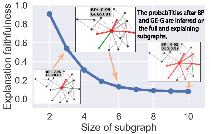
Explanation for Ratification One of the goals of explanations is to help end-users understand why the probabilistic beliefs are appropriate given the MRF, so that they can develop confidence in the beliefs and BP. This process is called “ratification” [41]. To attain this goal, Fig. 7 displays multiple explanations (trees) generated by Comb on the Karate Club network, with increasing size in Fig. 7 along with the faithfulness measured by the distance from Eq. (4). One can see that the distance decreases exponentially fast as more nodes are added to the explanation. On each explaining subgraph (tree), we display beliefs found by BP on $\mathchar 28999$ and $\tilde{\mathchar 28999}$ so that the user is aware of the gap. Since insight is personal [41], the interface is endowed with flexibility for a user to navigate through alternatives, and use multiple metrics (distributional distance, subgraph size and topology) to select the more sensible ones. This design also allows the user to see how adding or removing an variable can alter the target belief, leading to more insight into and trust on the BP.

Explanation for Verification MRF designers can use the explanations for verification of their design, including network parameters and topology. We demonstrate how to use the generated subgraphs to identify a security issue in spam detection. Specifically, we desire that a spam review should be detected with equal probability by the same spam detector, regardless of how many reviews their authors have posted. On the one hand, it has been found that well-camouflaged elite spammer accounts can deliver better rating promotion [27], a fact that has been exploited by dedicated spammers [49]. On the other hand, a spam detector can be accurate in detecting fake reviews for the wrong reason, such as the prolificacy of the reviewers [36].

We gather all reviews from the YelpChi dataset, and from the generated subgraph explanations, create four features, including whether a review is connected to its reviewer and target product, and the degree of its two potential neighbors. We then train a logistic regression model on these features to predict the probability of a review being a false positive (4,501), a false negative (6,681), and mis-classified (11,182), using predictions based on SpEagle [34]. The point is that the above mistakes should not depend on the prolificacy of the connected reviewers and products. However, we found that a sizable subset of false negatives (1,153 out of 6,681) are due to the influence from the review node only based on our explanations. Moreover, the logistic model shows that the influence of the degree of the neighboring reivewer contributes the most to the probability of FN. This is a serious security issue: a spam from an prolific reviewers is more likely to be missed by SpEagle.

References

- [1] Edoardo Amaldi and Viggo Kann. On the approximability of minimizing nonzero variables or unsatisfied relations in linear systems. Theoretical Computer Science, 209(1-2):237–260, 1998.
- [2] David Baehrens, Timon Schroeter, Stefan Harmeling, Motoaki Kawanabe, Katja Hansen, and Klaus-Robert MÞller. How to explain individual classification decisions. Journal of Machine Learning Research, 11(Jun):1803–1831, 2010.
- [3] Dhruv Batra, Payman Yadollahpour, Abner Guzman-Rivera, and Gregory Shakhnarovich. Diverse m-best solutions in markov random fields. In European Conference on Computer Vision, pages 1–16. Springer, 2012.
- [4] Rich Caruana, Hooshang Kangarloo, JD Dionisio, Usha Sinha, and David Johnson. Case-based explanation of non-case-based learning methods. In Proceedings of the AMIA Symposium, page 212. American Medical Informatics Association, 1999.
- [5] Hei Chan and Adnan Darwiche. Sensitivity analysis in markov networks. In International Joint Conference on Artificial Intelligence, volume 19, page 1300. LAWRENCE ERLBAUM ASSOCIATES LTD, 2005.
- [6] Jonathan Chang, Sean Gerrish, Chong Wang, Jordan L Boyd-Graber, and David M Blei. Reading tea leaves: How humans interpret topic models. In Advances in neural information processing systems, pages 288–296, 2009.
- [7] Adnan Darwiche. A differential approach to inference in bayesian networks. Journal of the ACM (JACM), 50(3):280–305, 2003.
- [8] Jerome Friedman, Trevor Hastie, and Robert Tibshirani. Sparse inverse covariance estimation with the graphical lasso. Biostatistics, 9(3):432–441, 2008.
- [9] Joseph Gonzalez, Yucheng Low, and Carlos Guestrin. Residual splash for optimally parallelizing belief propagation. In Artificial Intelligence and Statistics, pages 177–184, 2009.
- [10] Bryce Goodman and Seth Flaxman. European union regulations on algorithmic decision-making and a “right to explanation”. AI Magazine, 38(3):50–57, 2017.
- [11] Isabelle Guyon and André Elisseeff. An introduction to variable and feature selection. Journal of machine learning research, 3(Mar):1157–1182, 2003.
- [12] Tamir Hazan and Amnon Shashua. Norm-product belief propagation: Primal-dual message-passing for approximate inference. IEEE Transactions on Information Theory, 56(12):6294–6316, 2010.
- [13] Jean Honorio, Dimitris Samaras, Irina Rish, and Guillermo Cecchi. Variable selection for gaussian graphical models. In Artificial Intelligence and Statistics, pages 538–546, 2012.
- [14] Qiang Huang, Ling-Yun Wu, and Xiang-Sun Zhang. An efficient network querying method based on conditional random fields. Bioinformatics, 27(22):3173–3178, 2011.
- [15] Saehan Jo, Jaemin Yoo, and U Kang. Fast and scalable distributed loopy belief propagation on real-world graphs. In Proceedings of the Eleventh ACM International Conference on Web Search and Data Mining, pages 297–305. ACM, 2018.
- [16] Matthew Johnson, David K Duvenaud, Alex Wiltschko, Ryan P Adams, and Sandeep R Datta. Composing graphical models with neural networks for structured representations and fast inference. In Advances in neural information processing systems, pages 2946–2954, 2016.
- [17] U Kang, Duen Horng, et al. Inference of beliefs on billion-scale graphs. 2010.
- [18] Ross Kindermann. Markov random fields and their applications. American mathematical society, 1980.
- [19] Pang Wei Koh and Percy Liang. Understanding black-box predictions via influence functions. In Proceedings of the 34th International Conference on Machine Learning-Volume 70, pages 1885–1894. JMLR. org, 2017.
- [20] Daphne Koller and Nir Friedman. Probabilistic graphical models: principles and techniques. MIT press, 2009.
- [21] Viktoriya Krakovna and Finale Doshi-Velez. Increasing the interpretability of recurrent neural networks using hidden markov models. arXiv preprint arXiv:1606.05320, 2016.
- [22] Isaac Lage, Emily Chen, Jeffrey He, Menaka Narayanan, Been Kim, Sam Gershman, and Finale Doshi-Velez. An evaluation of the human-interpretability of explanation. arXiv preprint arXiv:1902.00006, 2019.
- [23] Tao Lei, Regina Barzilay, and Tommi Jaakkola. Rationalizing neural predictions. arXiv preprint arXiv:1606.04155, 2016.
- [24] Ming-Hui Li, Lei Lin, Xiao-Long Wang, and Tao Liu. Protein–protein interaction site prediction based on conditional random fields. Bioinformatics, 23(5):597–604, 2007.
- [25] Tania Lombrozo. The structure and function of explanations. Trends in cognitive sciences, 10(10):464–470, 2006.
- [26] Yin Lou, Rich Caruana, and Johannes Gehrke. Intelligible models for classification and regression. In Proceedings of the 18th ACM SIGKDD international conference on Knowledge discovery and data mining, pages 150–158. ACM, 2012.
- [27] Michael Luca. Reviews, reputation, and revenue: The case of yelp. com. Com (March 15, 2016). Harvard Business School NOM Unit Working Paper, (12-016), 2016.
- [28] George A Miller. The magical number seven, plus or minus two: Some limits on our capacity for processing information. Psychological review, 63(2):81, 1956.
- [29] Galileo Mark Namata, Stanley Kok, and Lise Getoor. Collective graph identification. In Proceedings of the 17th ACM SIGKDD international conference on Knowledge discovery and data mining, pages 87–95. ACM, 2011.
- [30] George L Nemhauser, Laurence A Wolsey, and Marshall L Fisher. An analysis of approximations for maximizing submodular set functions. Mathematical programming, 14(1):265–294, 1978.
- [31] Steven W Norton. An explanation mechanism for bayesian inferencing systems. In Machine Intelligence and Pattern Recognition, volume 5, pages 165–173. Elsevier, 1988.
- [32] Judea Pearl. Probabilistic reasoning in intelligent systems: networks of plausible inference. Elsevier, 2014.
- [33] Bryan Perozzi, Rami Al-Rfou, and Steven Skiena. Deepwalk: Online learning of social representations. In Proceedings of the 20th ACM SIGKDD international conference on Knowledge discovery and data mining, pages 701–710. ACM, 2014.
- [34] Shebuti Rayana and Leman Akoglu. Collective opinion spam detection: Bridging review networks and metadata. In Proceedings of the 21th acm sigkdd international conference on knowledge discovery and data mining, pages 985–994. ACM, 2015.
- [35] Marco Tulio Ribeiro, Sameer Singh, and Carlos Guestrin. Why should i trust you?: Explaining the predictions of any classifier. In Proceedings of the 22nd ACM SIGKDD international conference on knowledge discovery and data mining, pages 1135–1144. ACM, 2016.
- [36] Andrew Slavin Ross, Michael C Hughes, and Finale Doshi-Velez. Right for the right reasons: Training differentiable models by constraining their explanations. arXiv preprint arXiv:1703.03717, 2017.
- [37] Chris Russell. Efficient search for diverse coherent explanations. arXiv preprint arXiv:1901.04909, 2019.
- [38] Barbara G Ryder. Constructing the call graph of a program. IEEE Transactions on Software Engineering, (3):216–226, 1979.
- [39] Karen Simonyan, Andrea Vedaldi, and Andrew Zisserman. Deep inside convolutional networks: Visualising image classification models and saliency maps. arXiv preprint arXiv:1312.6034, 2013.
- [40] Simone Stumpf, Erin Sullivan, Erin Fitzhenry, Ian Oberst, Weng-Keen Wong, and Margaret Burnett. Integrating rich user feedback into intelligent user interfaces. In Proceedings of the 13th international conference on Intelligent user interfaces, pages 50–59. ACM, 2008.
- [41] Henri J Suermondt. Explanation in bayesian belief networks. 1993.
- [42] Charles Sutton, Andrew McCallum, et al. An introduction to conditional random fields. Foundations and Trends® in Machine Learning, 4(4):267–373, 2012.
- [43] Lei Tang and Huan Liu. Relational learning via latent social dimensions. In Proceedings of the 15th ACM SIGKDD international conference on Knowledge discovery and data mining, pages 817–826. ACM, 2009.
- [44] Wenbin Tang, Honglei Zhuang, and Jie Tang. Learning to infer social ties in large networks. In Joint european conference on machine learning and knowledge discovery in databases, pages 381–397. Springer, 2011.
- [45] Randy L Teach and Edward H Shortliffe. An analysis of physician attitudes regarding computer-based clinical consultation systems. Computers and Biomedical Research, 14(6):542–558, 1981.
- [46] Sandra Wachter, Brent Mittelstadt, and Chris Russell. Counterfactual explanations without opening the black box: Automated decisions and the gpdr. Harv. JL & Tech., 31:841, 2017.
- [47] Mike Wojnowicz, Ben Cruz, Xuan Zhao, Brian Wallace, Matt Wolff, Jay Luan, and Caleb Crable. “influence sketching”: Finding influential samples in large-scale regressions. In 2016 IEEE International Conference on Big Data (Big Data), pages 3601–3612. IEEE, 2016.
- [48] Chen Yanover, Talya Meltzer, and Yair Weiss. Linear programming relaxations and belief propagation–an empirical study. Journal of Machine Learning Research, 7(Sep):1887–1907, 2006.
- [49] Haizhong Zheng, Minhui Xue, Hao Lu, Shuang Hao, Haojin Zhu, Xiaohui Liang, and Keith Ross. Smoke screener or straight shooter: Detecting elite sybil attacks in user-review social networks. arXiv preprint arXiv:1709.06916, 2017.
- [50] Marinka Zitnik and Jure Leskovec. Predicting multicellular function through multi-layer tissue networks. Bioinformatics, 33(14):i190–i198, 2017.