Scattering of energetic electrons by heat-flux-driven whistlers in flares
Abstract
The scattering of electrons by heat-flux-driven whistler waves is explored with a particle-in-cell (PIC) simulation relevant to the transport of energetic electrons in flares. The simulation is initiated with a large heat flux that is produced using a kappa distribution of electrons with positive velocity and a cold return current beam. This system represents energetic electrons escaping from a reconnection-driven energy release site. This heat flux system drives large amplitude oblique whistler waves propagating both along and against the heat flux, as well as electron acoustic waves. While the waves are dominantly driven by the low energy electrons, including the cold return current beam, the energetic electrons resonate with and are scattered by the whistlers on time scales of the order of a hundred electron cyclotron times. Peak whistler amplitudes of and angles of with respect to the background magnetic field are observed. Electron perpendicular energy is increased while the field-aligned electron heat flux is suppressed. The resulting scattering mean-free-paths of energetic electrons are small compared with the typical scale size of energy release sites in flares, which might lead to the effective confinement of energetic electrons that is required for the production of very energetic particles.
Keywords:
flares — particle-in-cell simulation — whistler waves — space plasmaI Introduction
Magnetic reconnection is the driver of explosive energy release in the sun’s corona (Forbes 1988) and in plasma environments throughout the universe (Michel 1994). In solar flares electrons can have energies exceeding a MeV (Lin et al. 2003; Gary et al. 2018) and in astrophysical environments can reach a PeV (Abdo et al. 2011). An important question that arises in building a model for electron acceleration in the sun and elsewhere is how electrons remain within the region where magnetic energy is being released for a sufficiently long time to reach the energies seen in observations.
The magnetic energy release rate in flares is controlled by magnetic reconnection in which the upper limit on the rate of reconnection is of order of where is the local Alfvén speed. For typical parameters (, ) is around km/s. The scale size of magnetic energy release in large solar flares can reach km so energy release rates are tens of seconds. In the absence of a confinement mechanism the transit time of a relativistic electron out of this region is of the order of . Consistent with these estimates, the decay time of hard X-ray emission from flares exceeds the transit time of energetic electrons across the source by two orders of magnitude (Masuda et al. 1994; Krucker et al. 2007; Krucker et al. 2010).
Thus, some mechanism for electron confinement is necessary to hold electrons in the energy release zone for a long enough time to reach relativistic energies. Because the Larmor radius of even relativistic electrons is small ( for the given numbers), one possibility is a form of magnetic confinement. However, magnetic field lines that link flare energy release sites end either on the chromosphere or the solar wind so confinement is not effective unless the electrons can mirror. Significant mirroring of energetic electrons would require that their velocity have a large component perpendicular to the ambient magnetic field. Recent models of electron acceleration during reconnection suggest that electron energy gain is mostly parallel to and is dominated either by parallel electric fields or Fermi reflection (Drake et al. 2006; Dahlin et al. 2014; Dahlin et al. 2016). The consequence is that electron distribution functions are strongly anisotropic even in 3D reconnecting systems, which become turbulent with the development of multiple x-lines and chaotic magnetic fields (Dahlin et al. 2017).
There is evidence from RHESSI spacecraft observations that the electron energy flux in the source regions of flares can exceed that measured at the chromosphere by up to an order of magnitude (Simões et al. 2013). It has been suggested that double layers driven by the return current of cold electrons interacting with ambient ions would cause reflection of some hot electrons. However, since the resulting potential drop across the double layers scales like (Li et al. 2013; Li et al. 2014) with the temperature of hot escaping electrons, the amplitude of double layers is not sufficient to trap relativistic electrons. Further, the direct measurement of radio emission from gyro-synchrotron emission from energetic electrons in flares requires significant energy in the perpendicular motion of electrons (Gary et al. 2018). Thus, if the dominant acceleration mechanism of electrons in flares is parallel to the ambient magnetic field, a mechanism is required to scatter the parallel energy into perpendicular energy.
A potential scattering mechanism for energetic electrons is via oblique whistler waves (e.g. Artemyev et al. 2012; Artemyev et al. 2014). The whistler resonance condition with electrons is given by , where is the electron cyclotron frequency, is an integer that can take on positive and negative values (Krall & Trivelpiece 1986) and is the relativistic Lorentz factor. For typical waves with the resonant velocities are given by , where is the electron skin depth and is the electron Alfvén speed. Scattering by an oblique whistler at each resonance can be efficient. Furthermore when overlap of resonances occurs, scattering can be strongly increased for a large fraction of electrons. (Roberg-Clark et al. 2016; Karimabadi et al. 1992). Kinetic simulations with boundary conditions that impose a fixed temperature jump along an ambient magnetic field have established that in high systems the fluctuating magnetic field from whistlers is comparable to the initial ambient magnetic field, which is sufficient to strongly scatter electrons. This limits their effective streaming velocity to the whistler phase speed, which in a system is of order .
In these previous works treating high- systems (Roberg-Clark et al. 2018a; Roberg-Clark et al. 2018b; Komarov et al. 2018) the imposed electron distribution functions were Maxwellians with specified temperature jumps that drove a heat flux. Here we consider a system in which the heat flux arises from electrons with a distribution propagating in one direction and a cold electron beam that produces a return current. In this system oblique whistlers develop that propagate both along and against the heat flux. Oblique whistlers propagating along the direction of the heat flux are driven at early time by the “fan” instability of the (anomalous) cyclotron resonance (Kadomtsev & Pogutse 1968; Haber et al. 1978; Fülöp et al. 2006; Krafft & Volokitin 2010; Vasko et al. 2019; Verscharen et al. 2019). At later time the growth of parallel-propagating electron acoustic waves facilitates the extraction of energy from the bulk of the hot electrons in tandem with the oblique whistlers. Whistlers propagating against the heat flux are driven by the Landau resonance with the return current electrons. Both classes of whistlers resonate with and scatter the most energetic electrons in the tail of the distribution, reducing their heat flux and substantially increasing their velocity perpendicular to the magnetic field.
II Simulation Method
We carry out a two-dimensional (2D) simulation using the PIC code (Zeiler et al. 2002) to model energetic electrons and a cold return current electron beam. calculates particle trajectories using the relativistic Newton-Lorentz equations and the electromagnetic fields are advanced using Maxwell’s equations. An initially uniform magnetic field threads the plasma. is therefore the parallel velocity and and are the perpendicular velocities, while is the perpendicular spatial coordinate. Boundary conditions are periodic in and . The initial particle distribution function has two components. The first is a parallel () bi- distribution with temperatures ,
| (1) |
is the initial density of each of the electron components, is the gamma function,
| (2) |
are the effective thermal speeds, are the regular thermal speeds, is the Heaviside step function and is a parameter that tunes the steepness of the nonthermal tail of the distribution.
The second electron component is the cold return current beam (moving against ) which takes the form of a drifting isotropic Maxwellian,
| (3) |
where is the cold thermal speed and is a drift speed that ensures zero net current () in the initial state while the error function makes the density of hot and cold particles equal. This choice is motivated by observations of flares (Krucker et al. 2010; Oka et al. 2013) suggesting that the population of energetic electrons is large.
For the simulation presented we chose , , . While this is a relatively high for the corona , a system is consistent with specific flare observations (Krucker et al. 2010), is inferred more generally from rough equipartition of energy release between heated and energetic ions and electrons in flares (Emslie et al. 2005; Emslie et al. 2012), and is seen in reconnection simulations (Dahlin et al. 2017). The large value of is motivated by 3D PIC simulations of reconnection in Dahlin et al. 2017 showing . This system is marginally stable with respect to the fluid firehose criterion, i.e. .
The simulation domain lengths are and , where is the electron skin depth and is the electron plasma frequency. Other parameters in the simulation include , and , which sets . The characteristic velocity of whistlers depends on the wavelength but has an upper limit that scales with the electron Alfvén speed , where . Ions, with mass ratio , are initialized with a Maxwellian distribution of temperature and do not play a significant role in the simulation. The simulation uses particles per species per cell, has a grid of by cells, and is run to the time .
III Simulation Results
The initial distribution function [the total of Eqs. (1) and (3)] drives magnetic fluctuations unstable in the system. Shown in Fig. 1(a) is the time evolution of the box-averaged magnetic fluctuation energies and , where . The energy in peaks at around after a fast growth phase while a second peak occurs at . The magnetic fluctuations damp significantly by the end of the simulation, approaching early-time noise levels.
To establish that the growth of the fluctuations is associated with the scattering of electrons, we track the time dependence of the electron distribution function , with as well as the two spatial coordinates averaged out. We use and as proxies for the parallel and perpendicular velocities since and the distribution remains gyrotropic for the duration of the simulation (not shown). We divide velocity space into ranges of width , treating as the total velocity. In Fig. 1(b) the time dependence of is shown for each velocity range with labels indicating the velocity intervals. For each of the energy ranges increases with time. Figure 2 reveals that the distribution of energy is almost unchanged during the course of the simulation since the initial and late-time distributions (at and ) basically overlap for most energies (and only vary slightly at high energy where there are few particles). Thus, the increase in in time corresponds to a decrease in so the dominant scattering is in pitch angle. The sharpest increase in occurs at around . The characteristic time over which increases is roughly , which we take to be the scattering time of the electrons. Saturation of (the “rollover”) takes place for a long period of time starting around and continues until the end of the simulation.
Scattering of the energy from to also reduces the energy flux, which is shown in Fig. 1(c) where we plot the time dependence of for the same energy bins as in Fig. 1b. Note that the data is presented on a log scale and we do not divide by the number of particles in each velocity range for this quantity. Curves representing most of the velocity ranges show a monotonic decrease of with time, in some cases resulting in a drop by a factor of . An exception is the curve corresponding to which increases until it peaks at and then drops off.
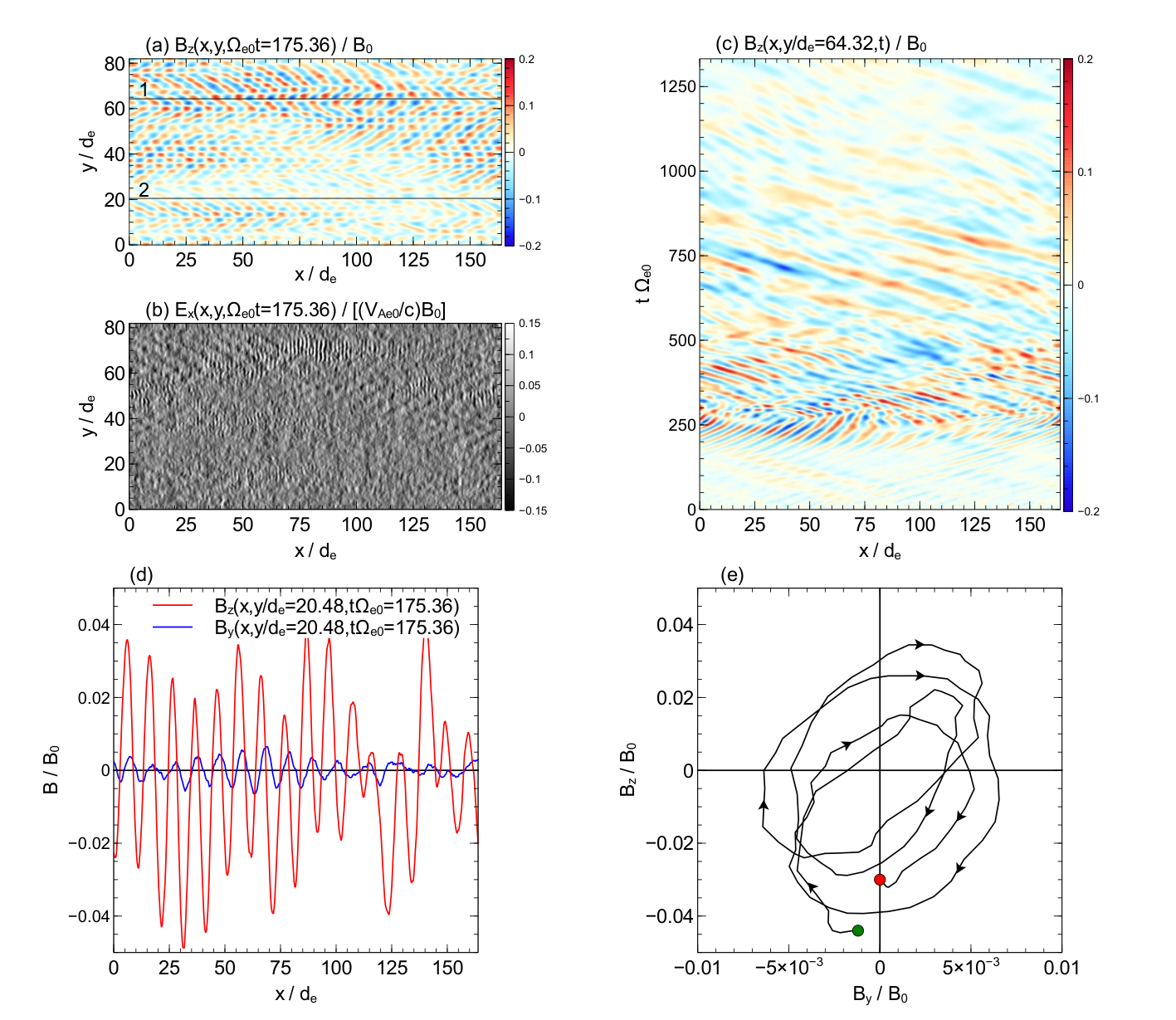
To establish the nature of the fluctuations that develop in the simulation we show in Fig. 3 the structure and motion of the out-of-plane magnetic fluctuations and the parallel electric field fluctuations . Figure 3a is a 2D plot of at early time, , during the first growth phase. The fluctuations travel at angles of roughly degrees relative to as predicted in Verscharen et al. 2019 for whistler scattering of energetic particles in a low- system. The Verscharen et al. result is constrained by the location of the resonance and a minimization of Landau damping, which is ensured if the whistler phase speed is large enough compared to the core electron thermal speed. In our simulation, however, the particle distribution is flat in near the whistler phase speed and so the whistler does not suffer from large Landau damping in the case. Rather, the angle of maximizes the wave-particle interaction for the resonance (equation 6). The crossed interference pattern that emerge in the simulation seem to be a consequence of the symmetry between the plus and minus directions. For every oblique wave generated with a velocity in the plus direction, there will be a companion wave with a velocity in the negative direction, which leads to a standing-wave-like pattern. Spatial inhomogeneities in the wave pattern are probably due to variations in noise levels in the system at early time.
A spacetime diagram of at a cut at is shown in Fig. 3c. Waves moving in the direction become visible around (recall the first peak in the fluctuating in Fig. 1b at ) but are beginning to slow down and reverse their direction by this time. The parallel phase speed of these waves at early time () is while at later time the leftward-propagating waves move at roughly with noticeably longer parallel wavelengths.
In Fig. 3d are plots of and along a cut at revealing what appears to be a degree phase shift between the two components. We also show a hodogram of these quantities from to in Fig. 3e demonstrating right-handed elliptical polarization, confirming that these are indeed whistlers.
The cold plasma dispersion relation for whistlers (neglecting the displacement current) is
| (4) |
with () corresponding to a “rightward” (“leftward”) whistler propagating along (against) . From Eq. (4) the phase speed of seen at early time in the simulation corresponds to a wave with , a value that is consistent with the wavelength of fluctuations in Fig. 3a. The fluctuations in the electric field at (Fig. 3b) show crossed patterns similar to those in 3a. These are the parallel electric fields of the rightward moving oblique whistlers, which are significant for large oblique angles and for . In Fig. 3b there are shorter-wavelength, parallel-propagating modes with and which are electron acoustic waves (EAWs) [ is the electron Debye length]. The waves grow through the Landau resonance between the thermal speeds of the hot and cold electron components and reduce the relative drift between those components (Gary & Tokar 1985; Agapitov et al. 2018; Vasko et al. 2018). These modes are of large amplitude, (note Fig. 3b has its color scale capped at to bring out the whistler signal).

Figures 4a-c illustrate the scattering of the electron distribution function as time proceeds in the simulation. The color plot shows the contours of constant . At (Fig. 4a) the large discontinuity in at separates the return current beam with and the distribution with . At (Fig. 4b) the distribution develops horn-like structures near and that demonstrate that particles from the initial distribution near the =0 axis have been scattered to higher and lower . The largest number of scattered particles is in the structure at . The discontinuity in Fig. 4a has been filled in and the contours of the distribution are fairly flat in the vicinity of the whistler phase speed . We attribute the flattening to large-amplitude electrostatic fluctuations that quickly grow up and damp in the simulation (not shown). When (4c), the distribution is significantly more isotropic in the half-plane. While some particles have been scattered to , most of the scattering seems to be limited to , suggesting that saturates in Fig. 1a because the half-plane has become nearly isotropic. Figure 4c is therefore representative of the late-time structure of the distribution function.
IV Resonances
To explain scattering in the simulation we invoke the basic theory of resonant interaction between oblique whistlers and electrons (see e.g. Roberg-Clark et al. 2016 and references therein). We write the resonance condition as
| (5) |
where , is the parallel resonant velocity, and with the total electron velocity. We first discuss the non-relativistic case () for which the resonance is represented by a vertical line in the space. In the long-wavelength limit, , the electric field of a single whistler is eliminated in a frame moving along at the speed . Energy conservation, , then requires that particle orbits lie on circles centered around as they oscillate in the fields of the whistler. When the whistler retains a finite electric field in its frame and particle energy is not exactly conserved (Karimabadi et al. 1990; Karimabadi et al. 1992). The nonlinear trapping width associated with a resonance can be calculated from the electron equation of motion in the whistler frame. Using the linearized cold plasma dispersion relation to obtain the whistler field components (neglecting the displacement current) we find the parallel trapping width of the th resonance to be
| (6) |
where is the Bessel function of order n, is the initial perpendicular velocity of the particle as it becomes resonant, and the whistler eigenvector amplitude is that of . Figure 5 shows a schematic of the trapping widths for the resonances with , , which is the location of the peak in the spectrum obtained from the FFT of at (not shown). The peak whistler amplitude of is chosen to evaluate the trapping widths. The trapping widths in are comparable to for .
Figure 5 establishes that the resonance strongly scatters particles with , producing the large horn-like feature near in Fig. 4b and transferring energy from the particles to the wave. The horn-like feature could also explain why the heat flux of the lowest-energy particles in Fig. 1 peaks for since initially higher-energy particles could be scattered into the lowest velocity bin. The resonance scatters some of the particles in the return current beam with to higher and smaller (note the small horn-like feature at this location in Fig. 4b). This interaction has a damping effect on the wave but the drive from still dominates since the number of upscattered cold return current electrons is small. Initially the distribution function is flat near the whistler phase speed (Fig. 4) so any effect on the energy of the whistler by the resonance is small. As a result the fan instability associated with the resonance is what drives the wave at early time.
The rightward-moving electron acoustic waves (EAWs) in Fig. 3b are parallel-propagating, so only the Landau resonance is significant. It produces a trapping width
| (7) |
where is the EAW amplitude. Setting and (the peak amplitude observed) we find that the EAW Landau resonance width (indicated by green vertical lines) overlaps with that of the whistler (orange curves) for a region of the phase space near and nearly overlaps that of the resonance (blue curves) near . Such overlap should lead to irreversible diffusion in phase space, dragging particles towards as seen over time in Fig. 4(a-c). If the overlap is not quite reached between the two whistler resonances and that of the EAW, chaotic orbits will still set in as overlap is approached. A small spread in can also shift the centroids of the traps and bridge the gap between the resonances. Importantly, a particle’s energy can be reduced by a whistler and an EAW acting in tandem. The hornlike feature in Fig. 4b has been shifted to the EAW phase speed in Fig. 4c, pulling some particles into the whistler resonance at late time. This is a simple, graphical way to describe the nonlinear interaction of whistlers and EAWs (Agapitov et al. 2018; Vasko et al. 2018; Drake et al. 2015). The interaction between the whistler resonance and the EAW resonance is analogous to the upscattering of high-energy particles and subsequent driving of plasma waves via a bump-on-tail instability as discussed in Haber et al. 1978.
As particles lose energy and diffuse towards they also lose momentum. To maintain zero net current the system generates an inductive field that slows the average drift speed of the return current beam. The leftward moving whistler grows by drawing energy from the return current beam via the Landau resonance at the phase speed . The flattening of the distribution across in Fig. 4c is evidence that this is taking place. This leftward whistler does not grow at early time because of damping of this wave by particles at the resonance (Verscharen et al. 2019). At late time the electron distribution at this resonance has been flattened by the action of the rightward propagating whistler so growth of the negative propagating wave through the Landau resonance takes place. Note that the large number of particles in the return current means the dominant energy transfer to the leftward wave is through the Landau resonance, so it is a beam-driven mode.
V Relativistic effects
Since there are very few particles at high energy for the initial distribution function chosen for the simulation, the high-energy component basically act as test particles. Their feedback on the wave dynamics is small. For these particles relativistic effects are important. In the relativistic case () the resonant surfaces and constant energy surfaces become elliptical in the plane (Omidi & Gurnett 1982; Karimabadi et al. 1990). Trapping occurs around the intersection point of these two ellipses (Karimabadi et al. 1990), assuming that to lowest order in wave amplitude the particle energy is conserved in the wave frame.
Intersection of the resonance ellipse with the axis is given by
| (8) |
where and is calculated from Eq. (4). The constant-energy ellipses (Karimabadi et al. 1990) are given by
| (9) |
with , and the initial Lorentz factor of a particle in the lab frame. For the whistlers in the simulation with the and axes of the ellipses are nearly equal. In the highly relativistic limit () the surface is a circle centered around with radius as expected.
Figure 4b displays the location of the resonance intersections for through using (8) and nearby energy surfaces using (9) assuming for the rightward moving wave. The energy surfaces, the horn-like structures, and the resonance intersections line up surprisingly well, justifying the use of the relativistic theory and further confirming that the waves are whistlers. The through resonances are also shown for the leftward wave (, ) in Fig. 4c, along with two energy surfaces. Since the leftward wave is long-wavelength, only the Landau resonance acts on low-energy particles. Scattering by the normal resonances likely aids in the diffusion of high-energy particles although the bulk of the scattering has already taken place by the time the leftward wave has a large amplitude. The most significant relativistic effect is the location of the resonances in Fig. 4. Expressions for the relativistic trapping widths, which we do not invoke here, can be found in Karimabadi et al. 1990.
VI Discussion
We have found that energetic electrons escaping from a flare-like system with , which is expected from magnetic reconnection (Dahlin et al. 2017), efficiently drive whistler waves that scatter the escaping electrons. The whistlers pitch-angle scatter high-energy electrons on a rapid time scale of hundreds of cyclotron periods by means of cyclotron resonances, suppressing energy flux and increasing the perpendicular velocities of electrons. This is a local mechanism which can operate under the generic conditions of a reconnection-driven flare. Moderate reduction (up to a factor of two) of the field-aligned electron energy flux occurs. Since this scattering tends to increase perpendicular velocity, electrons will more effectively mirror when they encounter small-scale magnetic fluctuations in the corona or if they are accelerated towards the sun where the ambient magnetic field is stronger. Thus, this scattering mechanism will facilitate the confinement of energetic electrons in energy release sites in flares which is required for electrons to reach the relativistic velocities seen in observations (Lin et al. 2003; Krucker et al. 2010; Gary et al. 2018).
Although our model was designed to study flares, we point out some possible implications for transport into the outer corona and ultimately the solar wind. The fluctuations in our simulation damp out after scattering is complete. Nevertheless, the heat flux associated with the initial electron distribution is permanently reduced. We suggest on the basis of the present simulations that oblique waves could have grown to large amplitude either in the corona or in the solar wind in the outer reaches of the corona, scattered the electrons to reduce the heat flux and then died away, leaving a remnant reduced heat flux. We thus propose that the electron energy flux produced in the corona as a result of reconnection or other mechanisms could be suppressed by oblique whistlers, leading to marginally stable electron distributions that then propagate outward, leaving no trace of the self-generated turbulence that limited the heat flux. It has been shown that distribution functions can stream ballistically over several mean free paths before collisions dominate and the distribution becomes Maxwellian-like (Malkov 2017). Since the mean free path of the solar wind is roughly , the streaming of heat-flux-carrying distributions out of the corona is thus feasible.
There is mounting evidence that the electron heat flux in the solar wind is limited by whistlers in regions with large plasma (Tong et al. 2018). However, the large-amplitude, oblique whistlers that would limit the heat flux have not been measured in the solar wind at AU (Wilson et al. 2013; Lacombe et al. 2014; Stansby et al. 2016; Tong et al. 2019a; Tong et al. 2019b; Kuzichev et al. 2019), although some observations have implied effective pitch-angle scattering by whistlers with small angles relative to (Kajdič et al. 2016). Oblique whistler scattering of the solar wind strahl into the halo is currently under active investigation (e.g. Verscharen et al. 2019, Boldyrev & Horaites 2019, Vasko et al. 2019).
Our simulation addresses the limit of flares. However, for a lower simulation, whistler growth would be suppressed since less free energy would be available (Roberg-Clark et al. 2018b). Scattering would still be expected to occur and the mode would retain a finite angle to . Since the electron Alfvén speed would increase relative to the thermal speed () the whistler phase speed might lie farther out in the tail of the distribution, leading to scattering of the highest energy particles.
We caution that our simulation suffers from the usual constraints of particle-in-cell simulations such as small simulated domains and short time scales compared to relevant scales in the corona. The model heat flux distribution function we use also contains a very sharp gradient near . However, sharp gradients are likely to form during flares, during which particles are rapidly accelerated and our intent is to explore the possible mechanisms at play that would limit electron escape. Our model is relevant to weakly collisional plasmas and could also be applied to transport in astrophysical coronae and low-luminosity accretion flows.
References
- Abdo et al. (2011) Abdo, A. A., Ackermann, M., Ajello, M., et al. 2011, Science, 331, 739 LP
- Agapitov et al. (2018) Agapitov, O., Drake, J. F., Vasko, I., et al. 2018, Geophysical Research Letters, 45, 2168
- Artemyev et al. (2012) Artemyev, A., Agapitov, O., Breuillard, H., Krasnoselskikh, V., & Rolland, G. 2012, Geophysical Research Letters, 39, 2007
- Artemyev et al. (2014) Artemyev, A. V., Vasiliev, A. A., Mourenas, D., et al. 2014, Geophysical Research Letters, 41, 5727
- Boldyrev & Horaites (2019) Boldyrev, S., & Horaites, K. 2019, arXiv:1908.01902
- Dahlin et al. (2014) Dahlin, J. T., Drake, J. F., & Swisdak, M. 2014, Physics of Plasmas, 21, 092304
- Dahlin et al. (2016) —. 2016, Physics of Plasmas, 23
- Dahlin et al. (2017) —. 2017, Physics of Plasmas, 24, 092110
- Drake et al. (2015) Drake, J. F., Agapitov, O. V., & Mozer, F. S. 2015, Geophysical Research Letters, 42, 2563
- Drake et al. (2006) Drake, J. F., Swisdak, M., Che, H., & Shay, M. A. 2006, Nature, 443, 553
- Emslie et al. (2005) Emslie, A. G., Dennis, B. R., Holman, G. D., & Hudson, H. S. 2005, Journal of Geophysical Research: Space Physics, 110, 1
- Emslie et al. (2012) Emslie, A. G., Dennis, B. R., Shih, A. Y., et al. 2012, Astrophysical Journal, 759, doi:10.1088/0004-637X/759/1/71
- Forbes (1988) Forbes, T. G. 1988, in Astrophysics and Space Science Library book series (ASSL, volume 143)
- Fülöp et al. (2006) Fülöp, T., Pokol, G., Helander, P., & Lisak, M. 2006, Physics of Plasmas, 13, 062506
- Gary et al. (2018) Gary, D. E., Chen, B., Dennis, B. R., et al. 2018, The Astrophysical Journal, 863, 83
- Gary & Tokar (1985) Gary, S. P., & Tokar, R. L. 1985, Physics of Fluids, 28, 2439
- Haber et al. (1978) Haber, I., Huba, J. D., Palmadesso, P., & Papadopoulos, K. 1978, The Physics of Fluids, 21, 1013
- Kadomtsev & Pogutse (1968) Kadomtsev, B., & Pogutse, O. 1968, Soviet Journal of Experimental and Theoretical Physics, 26, 1146
- Kajdič et al. (2016) Kajdič, P., Alexandrova, O., Maksimovic, M., Lacombe, C., & Fazakerley, A. N. 2016, The Astrophysical Journal, 833, 172
- Karimabadi et al. (1990) Karimabadi, H., Akimoto, K., Omidi, N., & Menyuk, C. R. 1990, Physics of Fluids B, 2, 606
- Karimabadi et al. (1992) Karimabadi, H., Krauss-Varban, D., & Terasawa, T. 1992, Journal of Geophysical Research, 97, 13853
- Komarov et al. (2018) Komarov, S., Schekochihin, A. A., Churazov, E., & Spitkovsky, A. 2018, J. Plasma Phys, 84
- Krafft & Volokitin (2010) Krafft, C., & Volokitin, A. 2010, Physics of Plasmas, 17, 102303
- Krall & Trivelpiece (1986) Krall, N. A., & Trivelpiece, A. W. 1986, Principles of Plasma Physics (San Francisco Press)
- Krucker et al. (2010) Krucker, S., Hudson, H. S., Glesener, L., et al. 2010, The Astrophysical Journal, 714, 1108
- Krucker et al. (2007) Krucker, S., White, S. M., & Lin, R. P. 2007, The Astrophysical Journal, 669, 49
- Kuzichev et al. (2019) Kuzichev, I. V., Vasko, I. Y., Soto-Chavez, A. R., et al. 2019, The Astrophysical Journal, 882, 81
- Lacombe et al. (2014) Lacombe, C., Alexandrova, O., Matteini, L., et al. 2014, The Astrophysical Journal, 796
- Li et al. (2013) Li, T. C., Drake, J. F., & Swisdak, M. 2013, The Astrophysical Journal, 778, 144
- Li et al. (2014) —. 2014, The Astrophysical Journal, 793, 7
- Lin et al. (2003) Lin, R. P., Krucker, S., Hurford, G. J., et al. 2003, The Astrophysical Journal, 595, 69
- Malkov (2017) Malkov, M. A. 2017, Physical Review D, 95, 1
- Masuda et al. (1994) Masuda, S., Kosugi, T., Hara, H., Tsuneta, S., & Ogawara, Y. 1994, Nature, 371, 495
- Michel (1994) Michel, F. C. 1994, The Astrophysical Journal, 431, 397
- Oka et al. (2013) Oka, M., Ishikawa, S., Saint-Hilaire, P., Krucker, S., & Lin, R. P. 2013, Astrophysical Journal, 764, 4
- Omidi & Gurnett (1982) Omidi, N., & Gurnett, D. A. 1982, Journal of Geophysical Research, 87, 2377
- Roberg-Clark et al. (2016) Roberg-Clark, G. T., Drake, J. F., Reynolds, C. S., & Swisdak, M. 2016, Astrophys. J. Lett., 830, L9
- Roberg-Clark et al. (2018a) —. 2018a, Phys. Rev. Lett., 120, 035101
- Roberg-Clark et al. (2018b) Roberg-Clark, G. T., Drake, J. F., Swisdak, M., & Reynolds, C. S. 2018b, The Astrophysical Journal, 867, 154
- Simões et al. (2013) Simões, P. J., Fletcher, L., Hudson, H. S., & Russell, A. J. 2013, Astrophysical Journal, 777, 1
- Stansby et al. (2016) Stansby, D., Horbury, T. S., Chen, C. H. K., & Matteini, L. 2016, The Astrophysical Journal, 829, L16
- Tong et al. (2018) Tong, Y., Bale, S. D., Salem, C., & Pulupa, M. 2018, arXiv:1801.07694
- Tong et al. (2019a) Tong, Y., Vasko, I. Y., Artemyev, A. V., Bale, S. D., & Mozer, F. S. 2019a, The Astrophysical Journal, 878, 41
- Tong et al. (2019b) Tong, Y., Vasko, I. Y., Pulupa, M., et al. 2019b, The Astrophysical Journal Letters, 870, L6
- Vasko et al. (2018) Vasko, I. Y., Agapitov, O. V., Mozer, F. S., et al. 2018, Physical Review Letters, 120, 195101
- Vasko et al. (2019) Vasko, I. Y., Krasnoselskikh, V., Tong, Y., et al. 2019, The Astrophysical Journal, 871, L29
- Verscharen et al. (2019) Verscharen, D., Chandran, B. D. G., Jeong, S.-Y., et al. 2019, arXiv:1906.02832
- Wilson et al. (2013) Wilson, L. B., Koval, A., Szabo, A., et al. 2013, Journal of Geophysical Research: Space Physics, 118, 5
- Zeiler et al. (2002) Zeiler, A., Biskamp, D., Drake, J. F., et al. 2002, Journal of Geophysical Research, 107, 1230