跳到论文正文
W Papers独立论文阅读器 arXiv:1908.06465 论文正文 计算阅读时间 · 0%
引用这篇论文根据当前论文元数据生成,正式投稿前建议核对。


License: arXiv.org perpetual non-exclusive license
arXiv:1908.06465v2 [math.DS] 07 Sep 2019

Structural Instability of Semi-Siegel Hénon mapsThanks: M. Y. was partially supported by NSERC Discovery grant. J. Y. carried out part of this work as a visiting member of the Fields Institute for Mathematical Sciences.

Michael Yampolsky and Jonguk Yang
Abstract.

We show that the dynamics of sufficiently dissipative semi-Siegel complex Hénon maps with golden-mean rotation number is not JJ-stable in a very strong sense. By the work of Dujardin and Lyubich, this implies that the Newhouse phenomenon occurs for a dense GδG_{\delta} set of parameters in this family. Another consequence is that the Julia sets of such maps are disconnected for a dense set of parameters.

Foreword

Complex quadratic Hénon maps have emerged as the key object of study in multi-dimensional Complex Dynamics. They occupy a similar place to that of quadratic polynomials in one-dimensional dynamics. Indeed, highly dissipative Hénon maps are naturally seen as small perturbations of quadratics – and the underlying one-dimensional dynamics plays a major role in their study. As an example, Fornaess and Sibony [FoSi], and Hubbard and Oberste-Vorth [HuOV] studied highly dissipative Hénon maps with an attracting fixed point, and showed that the dynamics of such maps on the Julia set naturally projects on the dynamics of hyperbolic quadratic polynomials in the main component of the Mandelbrot set. Thus, the same topological model applies to the dynamics of all such two-dimensional maps. A parallel result for dissipative Hénon maps with a semi-parabolic fixed point (that is, having an eigenvalue of the form e2​π​i​r,r∈ℚe^{2\pi ir},\;r\in{\mathbb{Q}}) was later proven by Radu and Tanase [RaTa].

In the present paper we consider another type of examples with a semi-neutral fixed point, the semi-Siegel dissipative Hénon maps. In the case when the neutral eigenvalue is equal to e2​π​i​re^{2\pi ir}, where r=(5+1)/2r=(\sqrt{5}+1)/2 is the golden mean, Gaidashev, Radu, and the first author [GaRaYam] recently showed that the Siegel disk of the Hénon map is bounded by a topological circle. This could be seen as a natural step towards describing the topological model of the dynamics of the two-dimensional map – and leads to asking whether it is again fibered over the underlying one-dimensional dynamics.

As we will see, this is not the case. In fact, semi-Siegel Hénon maps with golden-mean rotation numbers are structurally unstable in a very strong sense. The precise formulation of our result follows below. Combined with the work of Dujardin and Lyubich, our result has two interesting, previously unknown corollaries. First, the Newhouse phenomenon occurs for a dense GδG_{\delta} set of parameters in the semi-Siegel Hénon family. Second, for a dense set of parameters values, the golden-mean semi-Siegel Hénon Julia set is disconnected.

Acknowledgement

We would like to thank E. Bedford, M. Martens, and R. Radu for helpful discussions. We are grateful to R. Dujardin for pointing out the connections to his work with M. Lyubich, which enabled us to strengthen the results in an earlier version of this work.

1. Introduction

Consider the complex quadratic Hénon family:

Fc,a​(x,y):=(x2+c−a​y,x)for ​c∈ℂ​ and ​a∈ℂ∖{0}.F_{c,a}(x,y):=(x^{2}+c-ay,x)\hskip 14.22636pt\text{for }c\in\mathbb{C}\text{ and }a\in\mathbb{C}\setminus\{0\}.

For a≠0a\neq 0, the map Fc,aF_{c,a} is an automorphism of ℂ2{\mathbb{C}}^{2} with a constant Jacobian:

Jac⁡Fc,a≡a.\operatorname{Jac}F_{c,a}\equiv a.

Furthermore, we have

Fc,a​(x,y)→(fc​(x),x)asa→0,F_{c,a}(x,y)\to(f_{c}(x),x)\hskip 14.22636pt\text{as}\hskip 14.22636pta\to 0,

where

fc​(x):=x2+cfor ​c∈ℂf_{c}(x):=x^{2}+c\hskip 14.22636pt\text{for }c\in{\mathbb{C}}

is the standard one-dimensional quadratic family. In this paper, we will always assume that Fc,aF_{c,a} is a sufficiently dissipative map (i.e. |a|<ϵ¯≪1|a|<\bar{\epsilon}\ll 1).

As is common, will refer to the xx coordinate of a point in (x,y)∈ℂ2(x,y)\in{\mathbb{C}}^{2} as “horizontal”, and the yy coordinate as “vertical”. Figure 1 gives an intuition on how vertical and horizontal planes are mapped by a Hénon map.

Refer to caption
Figure 1. A Hénon map Fc,aF_{c,a}. Note that the xx-coordinate plane is mapped to the graph of fcf_{c}, and that the vertical planes are scaled uniformly by −a-a, and then mapped to horizontal planes.

In one-dimensional dynamics, the filled Julia set is defined as the set of points with bounded orbits. Since Fc,aF_{c,a} is an automorphism, the analogous definitions are made both for forward and for backward orbits:

K±​(Fc,a):={𝐱∈ℂ2|{Fc,a±n​(𝐱)}n∈ℕ​ is bounded};K^{\pm}(F_{c,a}):=\{{\mathbf{x}}\in{\mathbb{C}}^{2}\,|\,\{F_{c,a}^{\pm n}({\mathbf{x}})\}_{n\in{\mathbb{N}}}\text{ is bounded}\};

the intersection of these sets is denoted by

K⁡(Fc,a):=K+​(Fc,a)∩K−​(Fc,a).K(F_{c,a}):=K^{+}(F_{c,a})\cap K^{-}(F_{c,a}).

The forward and backward Julia sets are

J±​(Fc,a):=∂K±​(Fc,a),J^{\pm}(F_{c,a}):=\partial K^{\pm}(F_{c,a}),

and the Julia set is defined as

J⁡(Fc,a):=J+​(Fc,a)∩J−​(Fc,a).J(F_{c,a}):=J^{+}(F_{c,a})\cap J^{-}(F_{c,a}).

Let 𝒮⁡(Fc,a){\mathcal{S}}(F_{c,a}) be the set of saddle periodic points of Fc,aF_{c,a}. For 𝐬∈𝒮⁡(Fc,a){\mathbf{s}}\in{\mathcal{S}}(F_{c,a}), we denote its stable and unstable manifold by Ws​(𝐬)W^{s}({\mathbf{s}}) and Wu​(𝐬)W^{u}({\mathbf{s}}) respectively. An intersection point 𝐪∈Ws​(𝐬1)∩Wu​(𝐬2){\mathbf{q}}\in W^{s}({\mathbf{s}}_{1})\cap W^{u}({\mathbf{s}}_{2}) with 𝐬1,𝐬2∈𝒮⁡(Fc,a){\mathbf{s}}_{1},{\mathbf{s}}_{2}\in{\mathcal{S}}(F_{c,a}) is said to be homoclinic if 𝐬1=𝐬2{\mathbf{s}}_{1}={\mathbf{s}}_{2}, and heteroclinic otherwise.

In dimension one, it is well-known that the set of repelling periodic points is dense in the Julia set of a rational map. This motivates the following alternate notion of the Julia set for Fc,aF_{c,a}:

J∗​(Fc,a):=𝒮⁡(Fc,a)¯⊂J⁡(Fc,a).J^{*}(F_{c,a}):=\overline{{\mathcal{S}}(F_{c,a})}\subset J(F_{c,a}).

It is an open problem (posed by J.H. Hubbard) whether J∗​(Fc,a)=J⁡(Fc,a)J^{*}(F_{c,a})=J(F_{c,a}).

1.1. J-stability

Consider a holomorphic family (Fλ)λ∈Λ(F_{\lambda})_{\lambda\in\Lambda} of dissipative Hénon maps Fλ=Fcλ,aλF_{\lambda}=F_{c_{\lambda},a_{\lambda}} (both λ↦cλ\lambda\mapsto c_{\lambda} and λ↦aλ\lambda\mapsto a_{\lambda} are holomorphic functions) over a connected complex manifold Λ\Lambda. We say that this family is JJ-stable if its members are topologically conjugate on JJ, and the conjugating map depends continuously on λ\lambda.

Recall that an (unbranched) holomorphic motion of a set X⊂ℂdX\subset{\mathbb{C}}^{d} over Λ\Lambda is a family of mappings ϕλ:X→ℂd\phi_{\lambda}:X\to{\mathbb{C}}^{d} such that

  1. i)

    ϕλ0≡IdX\phi_{\lambda_{0}}\equiv\operatorname{Id}_{X} for some λ0∈Λ\lambda_{0}\in\Lambda;

  2. ii)

    λ↦ϕλ​(x)\lambda\mapsto\phi_{\lambda}(x) is holomorphic for a fixed x∈Xx\in X; and

  3. iii)

    x↦ϕλ​(x)x\mapsto\phi_{\lambda}(x) is injective for a fixed λ∈Λ\lambda\in\Lambda.

If a family ϕλ\phi_{\lambda} satisfies i) and ii), but not iii), we say that it is a branched holomorphic motion. An unbranched or branched holomorphic motion is said to be equivariant if

ϕλ∘Fλ0​(x)=Fλ∘ϕλ​(x)forx∈X.\phi_{\lambda}\circ F_{\lambda_{0}}(x)=F_{\lambda}\circ\phi_{\lambda}(x)\hskip 14.22636pt\text{for}\hskip 14.22636ptx\in X.

The true power of holomorphic motions lies in their extension properties. For d=1d=1, we have the following classical result of Mañé-Sad-Sullivan and Lyubich [MSS, Lyu]:

Theorem 1.1 (λ\lambda-lemma).

An unbranched holomorphic motion of X⊂ℂX\subset{\mathbb{C}} extends continuously to an unbranched holomorphic motion of X¯\overline{X}.

Holomorphic motions were used in [MSS, Lyu] for studying JJ-stability in dimension one. Namely, suppose the repelling periodic points persist in a holomorphic family of rational maps. Then these points move holomorphically. Using the λ\lambda-lemma, this motion can be extended to the entire Julia set–thereby supplying the required continuously varying conjugacy map for structural stability.

In [DuLy], Dujardin and Lyubich carry out this approach in a higher dimensional setting. The principal difficulty there is that for d≥2d\geq 2, the λ\lambda-lemma is no longer true: an unbranched holomorphic motion of a set may not extend to its closure; and even if it does, the resulting motion of the closure may become branched. To allow for such a possibility, they define the following alternative notion of stability.

Definition 1.2 ([DuLy]).

A holomorphic family (Fλ)λ∈Λ(F_{\lambda})_{\lambda\in\Lambda} is weakly J∗J^{*}-stable if there exists an equivariant branched holomorphic motion of J∗​(Fλ)J^{*}(F_{\lambda}).

A map Fλ1F_{\lambda_{1}} and its corresponding parameter λ1∈Λ\lambda_{1}\in\Lambda are said to be weakly J∗J^{*}-stable if (Fλ)λ∈U(F_{\lambda})_{\lambda\in U} is weakly J∗J^{*}-stable for some neighborhood U⊂ΛU\subset\Lambda of λ1\lambda_{1}; otherwise, we say that (Fλ)λ∈Λ(F_{\lambda})_{\lambda\in\Lambda} bifurcates at λ1\lambda_{1}.

Theorem 1.3 ([DuLy]).

Let (Fλ)λ∈Λ(F_{\lambda})_{\lambda\in\Lambda} be a holomorphic family of dissipative Hénon maps. The following are equivalent:

  1. i)

    The family (Fλ)λ∈Λ(F_{\lambda})_{\lambda\in\Lambda} is weakly J∗J^{*}-stable.

  2. ii)

    The set J∗​(Fλ)J^{*}(F_{\lambda}) moves continuously in the Hausdorff topology.

  3. iii)

    The type of every periodic point does not change (saddle, attracting, semi-indifferent).

  4. iv)

    Every saddle point moves under an equivariant unbranched holomorphic motion.

  5. v)

    Every homoclinic or heteroclinic intersection point moves under an equivariant unbranched holomorphic motion. Consequently, any homoclinic or heteroclinic tangency must persist in the whole family.

Remark 1.4.

It is easy to see that structural JJ-stability (or even just structural J∗J^{*}-stability) implies weak J∗J^{*}-stability. However, it is not known whether the converse is true.

1.2. Stability in the attracting and semi-parabolic family

A Hénon map Fc,aF_{c,a} is determined uniquely by the multipliers μ\mu and ν\nu at a fixed point. In particular, we have:

a=μ​νandc=(1+μ​ν)​(μ2+ν2)−(μ2+ν2)2.a=\mu\nu\hskip 14.22636pt\text{and}\hskip 14.22636ptc=(1+\mu\nu)\left(\frac{\mu}{2}+\frac{\nu}{2}\right)-\left(\frac{\mu}{2}+\frac{\nu}{2}\right)^{2}.

When convenient, we will write Fμ,νF_{\mu,\nu} instead of Fc,aF_{c,a} to denote a Hénon map. Note that we have

Fμ,ν​(x,y)→(fμ​(x),x)asν→0,F_{\mu,\nu}(x,y)\to(f_{\mu}(x),x)\hskip 14.22636pt\text{as}\hskip 14.22636pt\nu\to 0,

where fμf_{\mu} denotes the quadratic polynomial that has a fixed point of multiplier μ\mu.

Suppose |ν|<1|\nu|<1. If |μ|≤1|\mu|\leq 1, then Fμ,νF_{\mu,\nu} can be classified into one of four types:

  1. i)

    attracting if |μ|<1|\mu|<1;

  2. ii)

    semi-parabolic if μ=e2​π​pq​i\mu=e^{2\pi\frac{p}{q}i} for some p/q∈ℚ/ℤp/q\in{\mathbb{Q}}/{\mathbb{Z}};

  3. iii)

    semi-Siegel if μ=e2​π​θ​i\mu=e^{2\pi\theta i} for some θ∈(ℝ∖ℚ)/ℤ\theta\in({\mathbb{R}}\setminus{\mathbb{Q}})/{\mathbb{Z}}, and Fμ,νF_{\mu,\nu} is locally linearizable at the fixed point; or

  4. iv)

    semi-Cremer if μ=e2​π​θ​i\mu=e^{2\pi\theta i} for some θ∈(ℝ∖ℚ)/ℤ\theta\in({\mathbb{R}}\setminus{\mathbb{Q}})/{\mathbb{Z}}, and Fμ,νF_{\mu,\nu} is not locally linearizable at the fixed point.

The dynamics of attracting or semi-parabolic Hénon maps are well-understood. In particular, the following results hold:

Theorem 1.5 ([FoSi, HuOV]).

Let μ0∈𝔻∖{0}\mu_{0}\in{\mathbb{D}}\setminus\{0\}. Then there exists ϵ¯>0\bar{\epsilon}>0 such that the holomorphic family (Fμ0,ν)ν∈𝔻ϵ¯∖{0}(F_{\mu_{0},\nu})_{\nu\in{\mathbb{D}}_{\bar{\epsilon}}\setminus\{0\}} of attracting Hénon maps is structurally JJ-stable.

Theorem 1.6 ([RaTa]).

Let μ0=ei​π​pq\mu_{0}=e^{i\pi\frac{p}{q}} for some p/q∈ℚ/ℤp/q\in{\mathbb{Q}}/{\mathbb{Z}}. Then there exists ϵ¯>0\bar{\epsilon}>0 such that the holomorphic family (Fμ0,ν)ν∈𝔻ϵ¯∖{0}(F_{\mu_{0},\nu})_{\nu\in{\mathbb{D}}_{\bar{\epsilon}}\setminus\{0\}} of semi-parabolic Hénon maps is structurally JJ-stable.

Remark 1.7.

In fact, for both attracting and semi-parabolic Hénon maps, an explicit topological model of JJ (as well as J+J^{+}) can be provided. For more details, see [FoSi], [HuOV] and [RaTa].

1.3. The golden-mean semi-Siegel Hénon family

Let θ∗:=(5−1)/2\theta_{*}:=(\sqrt{5}-1)/2 be the inverse golden mean rotation number. Let Fa=Fμ∗,νF_{a}=F_{\mu_{*},\nu} be the Hénon map such that

Jac⁡Fa≡a∈𝔻∖{0},\operatorname{Jac}F_{a}\equiv a\in{\mathbb{D}}\setminus\{0\},

and FaF_{a} has a fixed point 𝐱a∈ℂ2{\mathbf{x}}_{a}\in{\mathbb{C}}^{2} of multipliers μ∗:=e2​π​θ∗​i\mu_{*}:=e^{2\pi\theta_{*}i} and ν=a/μ∗\nu=a/\mu_{*}. Since θ∗\theta_{*} is of bounded type, FaF_{a} is locally linearizable at 𝐱a{\mathbf{x}}_{a}, and thus, 𝐱a{\mathbf{x}}_{a} is semi-Siegel. The holomorphic family (Fa)ν∈𝔻∖{0}(F_{a})_{\nu\in{\mathbb{D}}\setminus\{0\}} is referred to as the golden-mean semi-Siegel Hénon family.

By Siegel’s Theorem [Sieg], there exists a local biholomorphic change of coordinates ψa:(U,(0,0))→(V,𝐱a)\psi_{a}:(U,(0,0))\to(V,\mathbf{x}_{a}) such that

ψa−1∘Fa∘ψa​(x,y)=(μ∗​x,ν​y).\psi_{a}^{-1}\circ F_{a}\circ\psi_{a}(x,y)=(\mu_{*}x,\nu y).

Then ψa\psi_{a} can be biholomorphically extended to a map ψa:(𝔻×ℂ,(0,0))→(𝒞a,𝐱a)\psi_{a}:(\mathbb{D}\times{\mathbb{C}},(0,0))\rightarrow(\mathcal{C}_{a},\mathbf{x}_{a}) so that its image 𝒞a:=ψa​(𝔻×ℂ)\mathcal{C}_{a}:=\psi_{a}(\mathbb{D}\times{\mathbb{C}}) is maximal (see [MoNiTaUe]). We call 𝒞a\mathcal{C}_{a} the Siegel cylinder of FaF_{a}. Clearly, the orbit of every point in 𝒞a\mathcal{C}_{a} converges to the biholomorphically embedded disk 𝒟a:=ψa​(𝔻×{0})\mathcal{D}_{a}:=\psi_{a}(\mathbb{D}\times\{0\}). We call 𝒟a\mathcal{D}_{a} the Siegel disk of FaF_{a}. See Figure 2.

Figure 2. The Siegel cylinder 𝒞a\mathcal{C}_{a} and the Siegel disk 𝒟a\mathcal{D}_{a} of FaF_{a}.
Remark 1.8.

The Siegel cylinder 𝒞a{\mathcal{C}}_{a} is a connected component of the interior of K+​(Fa)K^{+}(F_{a}). Moreover, we have ∂𝒞a=J+​(Fa)\partial{\mathcal{C}}_{a}=J^{+}(F_{a}) (see [BeSm]). The Siegel disk 𝒟a{\mathcal{D}}_{a} is contained in KK.

The first author and D. Gaidashev developed a renormalization theory of Siegel dynamics that extended to higher dimensions (see [GaYam]). By applying this new tool, jointly with Radu, they proved the following result:

Theorem 1.9 ([GaRaYam]).

There exists ϵ¯>0\bar{\epsilon}>0 such that if b∈𝔻ϵ¯∖{0}b\in{\mathbb{D}}_{\bar{\epsilon}}\setminus\{0\}, then the boundary of the Siegel disk 𝒟a{\mathcal{D}}_{a} for FaF_{a} is a homeomorphic image of the circle. In fact, the linearizing map

ψa|y=0:𝔻×{0}→𝒟a\psi_{a}|_{y=0}:{\mathbb{D}}\times\{0\}\rightarrow{\mathcal{D}}_{a}

extends continuously and injectively to the boundary.

Remark 1.10.

The above theorem implies that the boundary of the Siegel disk ∂𝒟a\partial{\mathcal{D}}_{a} is the support of an ergodic invariant measure, and hence, by [Du], it must be contained in J∗​(Fa)J^{*}(F_{a})11 1 This was pointed out to us by R. Dujardin..

In [Yan1], the second author reformulated the renormalization theory of [GaYam] to obtain precise quantitative estimates. A summary of this work is given in Section 2. These estimates then led to the following results on the geometry of the Siegel boundary for Hénon maps.

Theorem 1.11 ([Yan1]).

There exists ϵ¯>0\bar{\epsilon}>0 such that if a1,a2∈𝔻ϵ¯∖{0}a_{1},a_{2}\in{\mathbb{D}}_{\bar{\epsilon}}\setminus\{0\} and |a1|≠|a2||a_{1}|\neq|a_{2}|, then Fa1F_{a_{1}} and Fa2F_{a_{2}} cannot be C1C^{1}-conjugate on the boundary of their respective Siegel disks.

Theorem 1.12 ([Yan2]).

There exists ϵ¯>0\bar{\epsilon}>0 such that the set of parameter values aa for which the boundary of the Siegel disk 𝒟a{\mathcal{D}}_{a} for FaF_{a} has unbounded geometry contains a dense GδG_{\delta} subset in the disc 𝔻ϵ¯∖{0}{\mathbb{D}}_{\bar{\epsilon}}\setminus\{0\}.

The results mentioned thus far are restricted to the boundary of the Siegel disk 𝒟a{\mathcal{D}}_{a}. In this paper, we extend our scope to the global behavior of FaF_{a} by studying the topological properties of the boundary of the entire Siegel cylinder 𝒞a{\mathcal{C}}_{a}. Our main result is the following.

Main Theorem.

There exists ϵ¯>0\bar{\epsilon}>0 such that the golden-mean semi-Siegel Hénon family FaF_{a} is not weakly J∗J^{*}-stable at every parameter a∈𝔻ϵ¯∖{0}a\in{\mathbb{D}}_{\bar{\epsilon}}\setminus\{0\}.

Combining our main theorem with the work of R. Dujardin and M. Lyubich, we are able to conclude the following two surprising facts about the semi-Siegel Hénon family. First, by Corollary 4.5 in [DuLy]:

Corollary 1.13.

There exists a dense GδG_{\delta} subset X⊂𝔻ϵ¯∖{0}X\subset{\mathbb{D}}_{\bar{\epsilon}}\setminus\{0\} such that FaF_{a} is a Newhouse automorphism (i.e. has infinitely many sinks) for a∈Xa\in X.

Second, by Theorem 5.7 in [DuLy]:

Corollary 1.14.

There exists a dense subset Y⊂𝔻ϵ¯∖{0}Y\subset{\mathbb{D}}_{\bar{\epsilon}}\setminus\{0\} such that J⁡(Fa)J(F_{a}) is disconnected for a∈Ya\in Y.

The strategy of the proof of the Main Theorem is as follows. Using renormalization, we obtain a precise description of the geometry of stable and unstable manifolds of saddles near a dynamically defined point on the boundary of the Siegel disc called the “fold”. It turns out that under a change in the Jacobian aa, the stable manifolds, which are nearly vertical, remain almost stationary while the unstable manifolds, which are “bent”, move analytically. Using this fact, we force a contradiction with Theorem 1.3 v).

Our approach was greatly inspired by the work of Lyubich and Martens, who used renormalization to prove a global topological instability in the family of real Feigenbaum Hénon maps (see [LyMa]).

2. Preliminaries

In this section, we provide a brief summary of the renormalization theory of semi-Siegel Hénon maps. See [Yan1] for complete details.

Let a∈𝔻ϵ¯∖{0}a\in{\mathbb{D}}_{\bar{\epsilon}}\setminus\{0\} for some ϵ¯>0\bar{\epsilon}>0 sufficiently small. Consider the Hénon map

Fa​(x,y)=[x2+ca−a​yx]F_{a}(x,y)=\begin{bmatrix}x^{2}+c_{a}-ay\\ x\end{bmatrix}

that has a Siegel disc 𝒟a⊂ℂ2{\mathcal{D}}_{a}\subset{\mathbb{C}}^{2} with rotation number θ∗=(5−1)/2\theta_{*}=(\sqrt{5}-1)/2. Representing θ∗\theta_{*} by an infinite continued fraction with positive terms, we have:

θ∗=11+11+….\theta_{*}=\cfrac{1}{1+\cfrac{1}{1+\ldots{}}}.

The nnth partial convergent of θ∗\theta_{*} is the rational number pn/qnp_{n}/q_{n} obtained by terminating the continued fraction of θ∗\theta_{*} after the nnth term. The denominators {qn}n=0∞\{q_{n}\}_{n=0}^{\infty} form the Fibonacci sequence:

q0=1,q1=1andqn+1=qn+qn−1forn≥1.q_{0}=1\hskip 14.22636pt,\hskip 14.22636ptq_{1}=1\hskip 14.22636pt\text{and}\hskip 14.22636ptq_{n+1}=q_{n}+q_{n-1}\hskip 14.22636pt\text{for}\hskip 14.22636ptn\geq 1. (2.1)

2.1. Definition of renormalization

Let Ω^0\hat{\Omega}_{0} and Γ^0\hat{\Gamma}_{0} be suitably chosen topological bidisks in ℂ2{\mathbb{C}}^{2} such that Ω^0∩Γ^0∋(0,0)\hat{\Omega}_{0}\cap\hat{\Gamma}_{0}\ni(0,0) and Ω^0∪Γ^0⊃∂𝒟a\hat{\Omega}_{0}\cup\hat{\Gamma}_{0}\supset\partial{\mathcal{D}}_{a}. The pair representation of FaF_{a} is given by

Σ^0=(A^0,B^0):=(Fa|Ω^0,Fa|Γ^0).\hat{\Sigma}_{0}=(\hat{A}_{0},\hat{B}_{0}):=(F_{a}|_{\hat{\Omega}_{0}},F_{a}|_{\hat{\Gamma}_{0}}).

Let

Φ0​(x,y):=(λ0​x,λ0​y),\Phi_{0}(x,y):=(\lambda_{0}x,\lambda_{0}y), (2.2)

where λ0:=ca\lambda_{0}:=c_{a}. Observe that

Φ0−1∘Fa∘Φ0​(0,0)=(1,0).\Phi_{0}^{-1}\circ F_{a}\circ\Phi_{0}(0,0)=(1,0).

The normalized pair representation of FaF_{a} is defined as

Σ0=(A0,B0):=(Φ0−1∘A^0∘Φ0,Φ0−1∘B^0∘Φ0).\Sigma_{0}=(A_{0},B_{0}):=(\Phi_{0}^{-1}\circ\hat{A}_{0}\circ\Phi_{0},\Phi_{0}^{-1}\circ\hat{B}_{0}\circ\Phi_{0}).

The nnth renormalization of FaF_{a}:

𝐑n​(Fa):=Σn=(An,Bn),{\mathbf{R}}^{n}(F_{a}):=\Sigma_{n}=(A_{n},B_{n}),

where

An​(x,y)=[an​(x,y)hn​(x,y)]andBn​(x,y)=[bn​(x,y)x],A_{n}(x,y)=\begin{bmatrix}a_{n}(x,y)\\ h_{n}(x,y)\end{bmatrix}\hskip 14.22636pt\text{and}\hskip 14.22636ptB_{n}(x,y)=\begin{bmatrix}b_{n}(x,y)\\ x\end{bmatrix},

is the pair of rescaled iterates of Σ0\Sigma_{0} defined inductively as follows. Denote

(an)y​(x):=an​(x,y),(a_{n})_{y}(x):=a_{n}(x,y),

and let

Hn+1​(x,y):=[(an)y−1​(x)y].H_{n+1}(x,y):=\begin{bmatrix}(a_{n})_{y}^{-1}(x)\\ y\end{bmatrix}.

Consider the non-linear change of coordinates defined as

Φn+1​(x,y):=Hn+1∘Λn+1,\Phi_{n+1}(x,y):=H_{n+1}\circ\Lambda_{n+1},

where

Λn+1​(x,y)=(λn+1​x+cn+1,λn+1​y)\Lambda_{n+1}(x,y)=(\lambda_{n+1}x+c_{n+1},\lambda_{n+1}y) (2.3)

is an affine rescaling map to be specified later. The pair Σn+1=(An+1,Bn+1)\Sigma_{n+1}=(A_{n+1},B_{n+1}) is defined as

An+1=Φn+1−1∘Bn∘An2∘Φn+1andBn+1=Φn+1−1∘Bn∘An∘Φn+1.A_{n+1}=\Phi_{n+1}^{-1}\circ B_{n}\circ A_{n}^{2}\circ\Phi_{n+1}\hskip 14.22636pt\text{and}\hskip 14.22636ptB_{n+1}=\Phi_{n+1}^{-1}\circ B_{n}\circ A_{n}\circ\Phi_{n+1}.
Lemma 2.1.

There exist topological discs Z,W,V⊂ℂZ,W,V\subset{\mathbb{C}} containing 00 such that the following holds. Denote

Vn:=λ1−1⋅…⋅λn−1​V,Ωn:=Z×VnandΓn:=W×Vn.V_{n}:=\lambda_{1}^{-1}\cdot\ldots\cdot\lambda_{n}^{-1}V\hskip 14.22636pt,\hskip 14.22636pt\Omega_{n}:=Z\times V_{n}\hskip 14.22636pt\text{and}\hskip 14.22636pt\Gamma_{n}:=W\times V_{n}.

Then for all n∈ℕn\in{\mathbb{N}} sufficiently large, AnA_{n} and BnB_{n} are bounded analytic maps that are well-defined on Ωn\Omega_{n} and Γn\Gamma_{n} respectively.

Lemma 2.2.

The dependence of Σn=(An,Bn)\Sigma_{n}=(A_{n},B_{n}) on yy decays super-exponentially fast. That is, we have

sup(x,y)∈Ω‖∂yAn​(x,y)‖<C​ϵ¯2nandsup(x,y)∈Γ‖∂yBn​(x,y)‖<C​ϵ¯2n.\sup_{(x,y)\in\Omega}\|\partial_{y}A_{n}(x,y)\|<C\bar{\epsilon}^{2^{n}}\hskip 14.22636pt\text{and}\hskip 14.22636pt\sup_{(x,y)\in\Gamma}\|\partial_{y}B_{n}(x,y)\|<C\bar{\epsilon}^{2^{n}}.

for some uniform constant C>0C>0.

The one-dimensional projections of AnA_{n}, BnB_{n} and Σn\Sigma_{n} are given by

ηn​(x):=an​(x,0),ξn​(x):=bn​(x,0)andζn:=(ηn,ξn)\eta_{n}(x):=a_{n}(x,0)\hskip 14.22636pt,\hskip 14.22636pt\xi_{n}(x):=b_{n}(x,0)\hskip 14.22636pt\text{and}\hskip 14.22636pt\zeta_{n}:=(\eta_{n},\xi_{n}) (2.4)

respectively. By Lemma 2.1, we see that ηn\eta_{n} and ξn\xi_{n} are bounded analytic functions defined on ZZ and WW respectively. Moreover, by Lemma 2.2, the dynamics of Σn\Sigma_{n} degenerates to that of ζn\zeta_{n} super-exponentially fast. It is shown in [Yan1] that ηn\eta_{n} and ξn\xi_{n} each have a unique simple critical point which are C​ϵ¯2nC\bar{\epsilon}^{2^{n}}-close to each other. We choose the normalizing constants λn\lambda_{n} and cnc_{n} in (2.3) so that

ξn​(0)=1andξn′​(0)=0.\xi_{n}(0)=1\hskip 14.22636pt\text{and}\hskip 14.22636pt\xi_{n}^{\prime}(0)=0.

2.2. Renormalization convergence

Let ζ∗=(η∗,ξ∗)\zeta_{*}=(\eta_{*},\xi_{*}) be the fixed point of the one-dimensional renormalization operator ℛ{\mathcal{R}} given in [GaYam]. In particular, we have

λ∗−1​η∗∘ξ∗∘η∗​(λ∗​x)=η∗​(x)andλ∗−1​η∗∘ξ∗​(λ∗​x)=ξ∗​(x),\lambda_{*}^{-1}\eta_{*}\circ\xi_{*}\circ\eta_{*}(\lambda_{*}x)=\eta_{*}(x)\hskip 14.22636pt\text{and}\hskip 14.22636pt\lambda_{*}^{-1}\eta_{*}\circ\xi_{*}(\lambda_{*}x)=\xi_{*}(x), (2.5)

where

λ∗:=η∗∘ξ∗​(0)∈𝔻\lambda_{*}:=\eta_{*}\circ\xi_{*}(0)\in{\mathbb{D}}

is the universal scaling factor.

Convergence under renormalization for semi-Siegel Hénon maps was first obtained in [GaYam]. For the renormalization operator 𝐑{\mathbf{R}} defined above, the proof of convergence is given in [Yan1].

Theorem 2.3.

As n→∞n\to\infty, we have the following convergences (each of which occurs at an exponential rate):

  1. (i)

    ζn=(ηn,ξn)→ζ∗=(η∗,ξ∗)\zeta_{n}=(\eta_{n},\xi_{n})\to\zeta_{*}=(\eta_{*},\xi_{*});

  2. (ii)

    λn→λ∗\lambda_{n}\to\lambda_{*}; and

  3. (iii)

    Φn→Φ∗\Phi_{n}\to\Phi_{*}, where

    Φ∗​(x,y):=[ϕ∗​(x)λ∗​y]=[η∗−1​(λ∗​x)λ∗​y].\Phi_{*}(x,y):=\begin{bmatrix}\phi_{*}(x)\\ \lambda_{*}y\end{bmatrix}=\begin{bmatrix}\eta_{*}^{-1}(\lambda_{*}x)\\ \lambda_{*}y\end{bmatrix}.

2.3. First return iterate

Define the nnth microscope map of depth kk by

Φnn+k:=Φn+1∘Φn+2∘…∘Φn+k.\Phi_{n}^{n+k}:=\Phi_{n+1}\circ\Phi_{n+2}\circ\ldots{}\circ\Phi_{n+k}.

Let

Ωnn+k:=Φnn+k​(Ωn+k)andΓnn+k:=Φnn+k​(Γn+k).\Omega_{n}^{n+k}:=\Phi_{n}^{n+k}(\Omega_{n+k})\hskip 14.22636pt\text{and}\hskip 14.22636pt\Gamma_{n}^{n+k}:=\Phi_{n}^{n+k}(\Gamma_{n+k}).

Observe that {Ωnn+k∪Γnn+k}k=0∞\{\Omega_{n}^{n+k}\cup\Gamma_{n}^{n+k}\}_{k=0}^{\infty} is a nested sequence of open sets. See Figure 3.

Proposition 2.4.

Let λ∗∈𝔻\lambda_{*}\in{\mathbb{D}} be the universal scaling factor. Then we have

‖D​Φnn+k‖≍|λ∗|k.\|D\Phi_{n}^{n+k}\|\asymp|\lambda_{*}|^{k}.

Consequently, there exists a point (κn,0)∈ℂ2(\kappa_{n},0)\in{\mathbb{C}}^{2}, called the nnth fold, such that

⋂k=0∞Φnn+k​((Z∪W)×V)={(κn,0)}.\bigcap_{k=0}^{\infty}\Phi_{n}^{n+k}((Z\cup W)\times V)=\{(\kappa_{n},0)\}.
Remark 2.5.

The fold is a dynamically defined point with the same combinatorial address as the critical value ξ∗​(0)=1\xi_{*}(0)=1 for the one-dimensional renormalization limit ζ∗=(η∗,ξ∗)\zeta_{*}=(\eta_{*},\xi_{*}). In [dCLyMa], its analog is referred to as the tip.
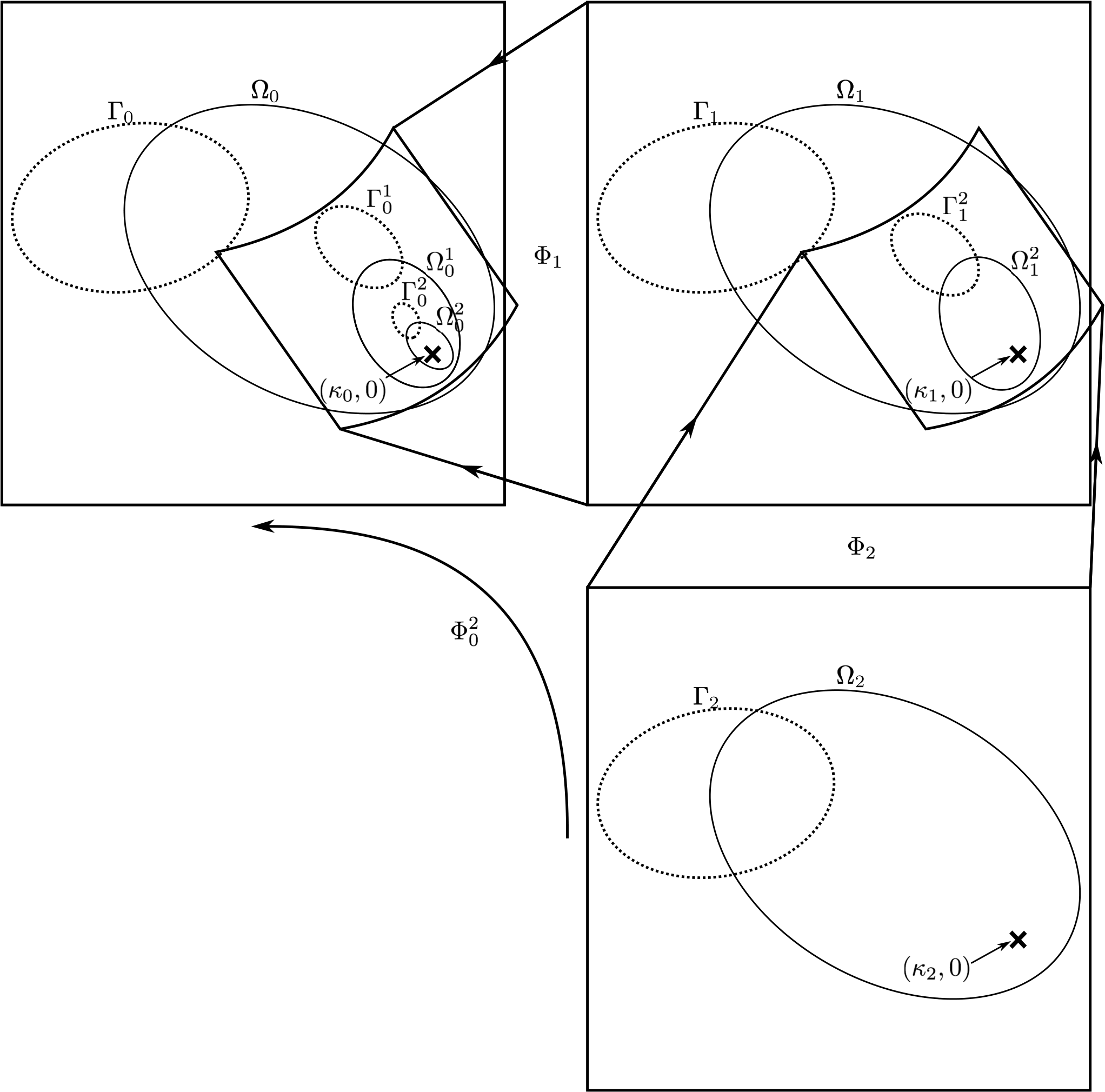
Refer to caption
Figure 3. The renormalization microscope map Φ02\Phi_{0}^{2} obtained by composing the non-linear changes of coordinates Φ1\Phi_{1} and Φ2\Phi_{2}. We have Ω01=Φ1​(Ω1)\Omega_{0}^{1}=\Phi_{1}(\Omega_{1}), Γ01=Φ1​(Γ1)\Gamma_{0}^{1}=\Phi_{1}(\Gamma_{1}), Ω02=Φ02​(Ω2)\Omega_{0}^{2}=\Phi_{0}^{2}(\Omega_{2}), Γ02=Φ02​(Γ2)\Gamma_{0}^{2}=\Phi_{0}^{2}(\Gamma_{2}), and (κ0,0)=Φ1​(κ1,0)=Φ02​(κ2,0)(\kappa_{0},0)=\Phi_{1}(\kappa_{1},0)=\Phi_{0}^{2}(\kappa_{2},0).

We denote by

p​Σnn+k=(p​Ann+k,p​Bnn+k)forn,k≥0p\Sigma_{n}^{n+k}=(pA_{n}^{n+k},pB_{n}^{n+k})\hskip 14.22636pt\text{for}\hskip 14.22636ptn,k\geq 0

the sequence of pairs of iterates of Σn=(An,Bn)\Sigma_{n}=(A_{n},B_{n}) defined inductively as follows:

  1. (i)

    p​Σnn:=Σnp\Sigma_{n}^{n}:=\Sigma_{n}, and

  2. (ii)

    p​Σnn+k+1:=(p​Bnn+k∘(p​Ann+k)2,p​Bnn+k∘p​Ann+k)p\Sigma_{n}^{n+k+1}:=(pB_{n}^{n+k}\circ(pA_{n}^{n+k})^{2},pB_{n}^{n+k}\circ pA_{n}^{n+k}).

It is not hard to see that we have

An+k=(Φnn+k)−1∘p​Ann+k∘Φnn+kandBn+k=(Φnn+k)−1∘p​Bnn+k∘Φnn+k.A_{n+k}=(\Phi_{n}^{n+k})^{-1}\circ pA_{n}^{n+k}\circ\Phi_{n}^{n+k}\hskip 14.22636pt\text{and}\hskip 14.22636ptB_{n+k}=(\Phi_{n}^{n+k})^{-1}\circ pB_{n}^{n+k}\circ\Phi_{n}^{n+k}. (2.6)

Moreover, by Lemma 2.1, p​Ann+kpA_{n}^{n+k} and p​Bnn+kpB_{n}^{n+k} are well-defined on Ωnn+k\Omega_{n}^{n+k} and Γnn+k\Gamma_{n}^{n+k} respectively.

Let

Ω^0n:=Φ0​(Ω0n)andΓ^0n:=Φ0​(Γ0n),\hat{\Omega}_{0}^{n}:=\Phi_{0}(\Omega_{0}^{n})\hskip 14.22636pt\text{and}\hskip 14.22636pt\hat{\Gamma}_{0}^{n}:=\Phi_{0}(\Gamma_{0}^{n}),

where Φ0\Phi_{0} is given in (2.2). By construction, the nnth renormalization

𝐑n​(Fa):=Σn=(An,Bn){\mathbf{R}}^{n}(F_{a}):=\Sigma_{n}=(A_{n},B_{n})

of FaF_{a} represents the first return map under FaF_{a} to the neighborhood Ω^0n∪Γ^0n\hat{\Omega}_{0}^{n}\cup\hat{\Gamma}_{0}^{n}. The following lemma is a formal statement of this fact.

Lemma 2.6.

Let {qn}n=0∞\{q_{n}\}_{n=0}^{\infty} be the Fibonacci sequence defined in (2.1). Define

p​A^0n:=Faq2​n+1|Ω^0nandp​B^0n:=Faq2​n|Γ^0n.p\hat{A}_{0}^{n}:=F_{a}^{q_{2n+1}}|_{\hat{\Omega}_{0}^{n}}\hskip 14.22636pt\text{and}\hskip 14.22636ptp\hat{B}_{0}^{n}:=F_{a}^{q_{2n}}|_{\hat{\Gamma}_{0}^{n}}.

Then

p​A0n=Φ0−1∘p​A^0n∘Φ0andp​B0n=Φ0−1∘p​B^0n∘Φ0.pA_{0}^{n}=\Phi_{0}^{-1}\circ p\hat{A}_{0}^{n}\circ\Phi_{0}\hskip 14.22636pt\text{and}\hskip 14.22636ptpB_{0}^{n}=\Phi_{0}^{-1}\circ p\hat{B}_{0}^{n}\circ\Phi_{0}.

Thus, Σn=(An,Bn)\Sigma_{n}=(A_{n},B_{n}) is given by

An=(Φ0n)−1∘Φ0−1∘p​A^0n∘Φ0∘Φ0nandBn=(Φ0n)−1∘Φ0−1∘p​B^0n∘Φ0∘Φ0n.A_{n}=(\Phi_{0}^{n})^{-1}\circ\Phi_{0}^{-1}\circ p\hat{A}_{0}^{n}\circ\Phi_{0}\circ\Phi_{0}^{n}\hskip 14.22636pt\text{and}\hskip 14.22636ptB_{n}=(\Phi_{0}^{n})^{-1}\circ\Phi_{0}^{-1}\circ p\hat{B}_{0}^{n}\circ\Phi_{0}\circ\Phi_{0}^{n}.

2.4. Limit of microscope maps

Let

ϕn​(x):=Φn​(x,0)andϕnn+k​(x):=Φnn+k​(x,0).\phi_{n}(x):=\Phi_{n}(x,0)\hskip 14.22636pt\text{and}\hskip 14.22636pt\phi_{n}^{n+k}(x):=\Phi_{n}^{n+k}(x,0).

It is not difficult to see that

ϕnn+k=ϕn+1∘ϕn+2​…​ϕn+k.\phi_{n}^{n+k}=\phi_{n+1}\circ\phi_{n+2}\ldots\phi_{n+k}.

Furthermore, we have

ϕn​(κn)=κn−1andϕnn+k​(κn+k)=κn,\phi_{n}(\kappa_{n})=\kappa_{n-1}\hskip 14.22636pt\text{and}\hskip 14.22636pt\phi_{n}^{n+k}(\kappa_{n+k})=\kappa_{n},

where (κn,0)(\kappa_{n},0) is the nnth fold given in Proposition 2.4. Denote

dn:=ϕn′​(κn)anddnn+k:=(ϕnn+k)′​(κn+k)=dn+1​dn+2​…​dn+k.d_{n}:=\phi_{n}^{\prime}(\kappa_{n})\hskip 14.22636pt\text{and}\hskip 14.22636ptd_{n}^{n+k}:=(\phi_{n}^{n+k})^{\prime}(\kappa_{n+k})=d_{n+1}d_{n+2}\ldots d_{n+k}.
Proposition 2.7.

The map ϕ∗:Z∪W→Z\phi_{*}:Z\cup W\to Z given in Theorem 2.3 has an attracting fixed point at 11 with multiplier λ∗2\lambda_{*}^{2}.

Proposition 2.8.

As n→∞n\to\infty, we have the following convergences (each of which occurs at an exponential rate):

  1. i)

    ϕn→ϕ∗\phi_{n}\to\phi_{*};

  2. ii)

    κn→1\kappa_{n}\to 1; and

  3. iii)

    dn→λ∗2d_{n}\to\lambda_{*}^{2}.

Let

ϕˇnn+k​(x):=ϕnn+k​(x+κn+k)−κnandϕˇ∗​(x):=ϕ∗​(x+1)−1.\check{\phi}_{n}^{n+k}(x):=\phi_{n}^{n+k}(x+\kappa_{n+k})-\kappa_{n}\hskip 14.22636pt\text{and}\hskip 14.22636pt\check{\phi}_{*}(x):=\phi_{*}(x+1)-1. (2.7)

Observe that ϕˇnn+k\check{\phi}_{n}^{n+k} and ϕˇ∗\check{\phi}_{*} both have an attracting fixed point at 00 of multiplier dnn+kd_{n}^{n+k} and λ∗2\lambda_{*}^{2} respectively.

Proposition 2.9.

We have the following convergence (which occurs at an exponential rate):

(dnn+k)−1​ϕˇnn+k→u∗ask→∞,(d_{n}^{n+k})^{-1}\check{\phi}_{n}^{n+k}\to u_{*}\hskip 14.22636pt\text{as}\hskip 14.22636ptk\to\infty,

where u∗u_{*} is the linearizing map for ϕˇ∗\check{\phi}_{*} at 00.

2.5. Universality

In [Yan1], the second author showed that the sequence of maps

𝐑n​(Fa)=Σn=(An,Bn){\mathbf{R}}^{n}(F_{a})=\Sigma_{n}=(A_{n},B_{n})

takes on a universal two-dimensional shape as it flattens and converges to the degenerate one-dimensional renormalization limit given in Theorem 2.3:

Theorem 2.10.

For n≥0n\geq 0, we have

Bn​(x,y)=[ξn​(x)−aq2​n​β​(x)​y​(1+O⁡(ρn))x],B_{n}(x,y)=\begin{bmatrix}\xi_{n}(x)-a^{q_{2n}}\,\beta(x)\,y\,(1+O(\rho^{n}))\\ x\end{bmatrix},

where 0<ρ<10<\rho<1 is a uniform constant; {qn}n=0∞\{q_{n}\}_{n=0}^{\infty} is the Fibonacci sequence; and β⁡(x)\beta(x) is a universal function that is uniformly bounded away from 00 and ∞\infty, and has a uniformly bounded derivative and distortion.

Theorem 2.11.

For n≥0n\geq 0, we have

An​(x,y)=[ηn​(x)−aq2​n​α​(x)​y​(1+O⁡(ρn))λn−1​η~n−1​(λn​x)−aq2​n​α~​(x)​y​(1+O⁡(ρn))],A_{n}(x,y)=\begin{bmatrix}\eta_{n}(x)-a^{q_{2n}}\,\alpha(x)\,y\,(1+O(\rho^{n}))\\ \lambda_{n}^{-1}\tilde{\eta}_{n-1}(\lambda_{n}x)-a^{q_{2n}}\,\tilde{\alpha}(x)\,y\,(1+O(\rho^{n}))\end{bmatrix},

where 0<ρ<10<\rho<1 is a uniform constant; {qn}n=0∞\{q_{n}\}_{n=0}^{\infty} is the Fibonacci sequence; and

η~k​(x)=ηk​(x)+O⁡(aq2​k),α⁡(x):=η∗′​(x)ξ∗′​(x)​β​(x)​and​α~​(x):=η∗′​(λ∗​x)η∗′​(x)​α​(x).\tilde{\eta}_{k}(x)=\eta_{k}(x)+O(a^{q_{2k}})\hskip 8.53581pt,\hskip 8.53581pt\alpha(x):=\frac{\eta_{*}^{\prime}(x)}{\xi_{*}^{\prime}(x)}\beta(x)\hskip 8.53581pt\text{and}\hskip 8.53581pt\tilde{\alpha}(x):=\frac{\eta_{*}^{\prime}(\lambda_{*}x)}{\eta_{*}^{\prime}(x)}\alpha(x).

Recall that we have

Φn​(κn,0)=(κn−1,0)andΦnn+k​(κn+k,0)=(κn,0).\Phi_{n}(\kappa_{n},0)=(\kappa_{n-1},0)\hskip 14.22636pt\text{and}\hskip 14.22636pt\Phi_{n}^{n+k}(\kappa_{n+k},0)=(\kappa_{n},0).

Denote

Dn:=D(κn,0)​ΦnandDnn+k:=D(κn+k,0)​Φnn+k=Dn+1⋅Dn+2⋅…⋅Dn+k.D_{n}:=D_{(\kappa_{n},0)}\Phi_{n}\hskip 14.22636pt\text{and}\hskip 14.22636ptD_{n}^{n+k}:=D_{(\kappa_{n+k},0)}\Phi_{n}^{n+k}=D_{n+1}\cdot D_{n+2}\cdot\ldots{}\cdot D_{n+k}.
Theorem 2.12.

Write

Dn=[1tn​aq2​(n−1)01]​[un00λn].D_{n}=\begin{bmatrix}1&t_{n}a^{q_{2(n-1)}}\\ 0&1\end{bmatrix}\begin{bmatrix}u_{n}&0\\ 0&\lambda_{n}\end{bmatrix}.

Then there exist a uniform positive constant ρ<1\rho<1 such that the following estimates hold for all n≥1n\geq 1:

  1. (i)

    un=λ∗2​(1+O⁡(ρn))u_{n}=\lambda_{*}^{2}(1+O(\rho^{n})),

  2. (ii)

    λn=λ∗​(1+O⁡(ρn))\lambda_{n}=\lambda_{*}(1+O(\rho^{n})), and

  3. (iii)

    tn=λ∗​α​(1)​(1+O⁡(ρn))t_{n}=\lambda_{*}\alpha(1)(1+O(\rho^{n})).

Consequently, for 0≤n,k0\leq n,k, we have

Dnn+k=[1tnn+k​aq2​n01]​[unn+k00λnn+k],D_{n}^{n+k}=\begin{bmatrix}1&t_{n}^{n+k}a^{q_{2n}}\\ 0&1\end{bmatrix}\begin{bmatrix}u_{n}^{n+k}&0\\ 0&\lambda_{n}^{n+k}\end{bmatrix},

where

  1. (i)

    unn+k:=un+1⋅un+1⋅…⋅un+k=λ∗2​k​(1+O⁡(ρn))u_{n}^{n+k}:=u_{n+1}\cdot u_{n+1}\cdot\ldots\cdot u_{n+k}=\lambda_{*}^{2k}(1+O(\rho^{n})),

  2. (ii)

    λnn+k:=λn+1⋅λn+2⋅…⋅λn+k=λ∗k​(1+O⁡(ρn))\lambda_{n}^{n+k}:=\lambda_{n+1}\cdot\lambda_{n+2}\cdot\ldots\cdot\lambda_{n+k}=\lambda_{*}^{k}(1+O(\rho^{n})), and

  3. (iii)

    tnn+k=tn+1​(1+O⁡(aq2​n+1))t_{n}^{n+k}=t_{n+1}(1+O(a^{q_{2n+1}})).

3. The Underlying One-Dimensional Dynamics

Consider the map ξn:W→ξn​(W)\xi_{n}:W\to\xi_{n}(W) given in (2.4). By Theorem 2.3, ξn\xi_{n} converges exponentially fast to ξ∗\xi_{*}, where ζ∗=(η∗,ξ∗)\zeta_{*}=(\eta_{*},\xi_{*}) is the fixed point of the one-dimensional renormalization operator ℛ{\mathcal{R}}.

Proposition 3.1.

The map ξn\xi_{n} has a unique repelling fixed point xˇn∈W\check{x}_{n}\in W. Moreover, xˇn\check{x}_{n} converges exponentially fast to the unique repelling fixed point x∗∈Wx_{*}\in W for ξ∗\xi_{*}.

Proof.

Proposition 3.2 of [Yam] implies that (ηn,ξn)(\eta_{n},\xi_{n}) forms a holomorphic pair in the sense of McMullen, with a priori bounds. By Denjoy-Wolff Theorem, ξn\xi_{n} has a unique fixed point in its domain of definition, which is attracting under ξn−1\xi_{n}^{-1}, and hence is repelling under ξn\xi_{n}. Finally, the exponential convergence statement follows by Proposition 3.1 of [Yam]. ∎

Let UnU_{n} be a small neighborhood of xˇn\check{x}_{n}, and denote:

ξnexp:=ξn|Un.\xi_{n}^{\exp}:=\xi_{n}|_{U_{n}}.

Then ξnexp\xi_{n}^{\exp} maps UnU_{n} conformally onto ξnexp​(Un)⋑Un\xi_{n}^{\exp}(U_{n})\Supset U_{n}. We may choose a domain 𝒰⊂W{\mathcal{U}}\subset W such that for all n∈ℕn\in{\mathbb{N}} sufficiently large, the following hold:

  1. i)

    xˇn∈𝒰\check{x}_{n}\in{\mathcal{U}};

  2. ii)

    (ξnexp)−1(\xi_{n}^{\exp})^{-1} extends to 𝒰{\mathcal{U}}; and

  3. iii)

    𝒰∖(ξnexp)−1​(𝒰)¯{\mathcal{U}}\setminus\overline{(\xi_{n}^{\exp})^{-1}({\mathcal{U}})} is a topological annulus containing 00.

Note that |(ξnexp)′​(x)|>C|(\xi_{n}^{\exp})^{\prime}(x)|>C for x∈(ξnexp)−1​(𝒰)x\in(\xi_{n}^{\exp})^{-1}({\mathcal{U}}) for some uniform constant C>0C>0.

Let Dδ​(0)D_{\delta}(0) be a disc of sufficiently small radius δ>0\delta>0 centered at 00. Recall that ξn:W→ξn​(W)\xi_{n}:W\to\xi_{n}(W) has a unique simple critical point at 00, and that ξn​(0)=1\xi_{n}(0)=1. It follows that ξn\xi_{n} has two distinct inverse branches on Dδ​(0)D_{\delta}(0), one of which is (ξnexp)−1(\xi_{n}^{\exp})^{-1}, and the other we denote by (ξnrot)−1(\xi_{n}^{\operatorname{rot}})^{-1}. Note that we have

(ξnexp)−1​(Dδ​(0))⊂(ξnexp)−1​(𝒰)and(ξnrot)−1​(Dδ​(0))∩𝒰=∅.(\xi_{n}^{\exp})^{-1}(D_{\delta}(0))\subset(\xi_{n}^{\exp})^{-1}({\mathcal{U}})\hskip 14.22636pt\text{and}\hskip 14.22636pt(\xi_{n}^{\operatorname{rot}})^{-1}(D_{\delta}(0))\cap{\mathcal{U}}=\varnothing.

See Figure 4.

Remark 3.2 (See Prop. 3.1 of [Yam]).

As n→∞n\to\infty, the maps (ξnexp)−1(\xi_{n}^{\exp})^{-1} and (ξnrot)−1(\xi_{n}^{\operatorname{rot}})^{-1} converge exponentially fast to two distinct inverse branches (ξ∗exp)−1(\xi_{*}^{\exp})^{-1} and (ξ∗rot)−1(\xi_{*}^{\operatorname{rot}})^{-1} of ξ∗\xi_{*}.

Figure 4. A choice of the domain 𝒰⊂W{\mathcal{U}}\subset W on which ξn\xi_{n} is uniformly expanding. The other branch (ξnrot)−1(\xi_{n}^{\operatorname{rot}})^{-1} maps the disc Dδ​(0)D_{\delta}(0) outside of 𝒰{\mathcal{U}}.
Theorem 3.3 ([Yan2]).

For n≥0n\geq 0, we have

An∘Φn+1​(x,y)=[λn+1​x+cn+1(ξ~nrot)−1​(λn+1​x)−aq2​n+1​β~​(x)​λn+1​y​(1+O⁡(ρn))],A_{n}\circ\Phi_{n+1}(x,y)=\begin{bmatrix}\lambda_{n+1}x+c_{n+1}\\ (\tilde{\xi}_{n}^{\operatorname{rot}})^{-1}(\lambda_{n+1}x)-a^{q_{2n+1}}\,\tilde{\beta}(x)\,\lambda_{n+1}\,y(1+O(\rho^{n}))\end{bmatrix},

where 0<ρ<10<\rho<1 is a uniform constant; {qn}n=0∞\{q_{n}\}_{n=0}^{\infty} is the Fibonacci sequence; and

(ξ~nrot)−1​(x)=(ξnrot)−1​(x)+O⁡(aq2​(n−1))​and​β~​(x):=ξ∗′​(λ∗​x)ξ∗′​(x)​β⁡(x)β⁡(λ∗​x).(\tilde{\xi}_{n}^{\operatorname{rot}})^{-1}(x)=(\xi_{n}^{\operatorname{rot}})^{-1}(x)+O(a^{q_{2(n-1)}})\hskip 8.53581pt\text{and}\hskip 8.53581pt\tilde{\beta}(x):=\frac{\xi_{*}^{\prime}(\lambda_{*}x)}{\xi_{*}^{\prime}(x)}\frac{\beta(x)}{\beta(\lambda_{*}x)}.

3.1. The degenerate map in dimension two

Consider the degenerate map Bˇn:Γn=W×Vn→Bˇn​(Γn)\check{B}_{n}:\Gamma_{n}=W\times V_{n}\to\check{B}_{n}(\Gamma_{n}) defined by

Bˇn​(x,y):=(ξn​(x),x).\check{B}_{n}(x,y):=(\xi_{n}(x),x).

By Proposition 3.1, we see that the map Bˇn\check{B}_{n} has a unique saddle point

𝐬ˇn:=(xˇn,xˇn)∈Γn⊂ℂ2\check{{\mathbf{s}}}_{n}:=(\check{x}_{n},\check{x}_{n})\in\Gamma_{n}\subset{\mathbb{C}}^{2}

with one multiplier the same as that of xˇn\check{x}_{n} for ξn\xi_{n}, and the other equal to 00. The local stable manifold of 𝐬ˇn\check{{\mathbf{s}}}_{n} can be identified with the vertical line segment through 𝐬ˇn\check{{\mathbf{s}}}_{n}:

ℳlocs​(𝐬ˇn):={(xˇn,y)|y∈Vn}.{\mathcal{M}}^{s}_{\operatorname{loc}}(\check{{\mathbf{s}}}_{n}):=\{(\check{x}_{n},y)\,|\,y\in V_{n}\}.

In other words, ℳlocs​(𝐬ˇn){\mathcal{M}}^{s}_{\operatorname{loc}}(\check{{\mathbf{s}}}_{n}) is the graph of the constant map

y↦xˇfory∈Vn.y\mapsto\check{x}\hskip 14.22636pt\text{for}\hskip 14.22636pty\in V_{n}.

The local unstable manifold of 𝐬ˇn\check{{\mathbf{s}}}_{n} can be identified with the following embedding of (ξnexp)−1​(𝒰)⊂ℂ(\xi_{n}^{\exp})^{-1}({\mathcal{U}})\subset{\mathbb{C}} into ℂ2{\mathbb{C}}^{2}:

ℳlocu​(𝐬ˇn):={(ξn​(x),x)|x∈(ξnexp)−1​(𝒰)}.{\mathcal{M}}^{u}_{\operatorname{loc}}(\check{{\mathbf{s}}}_{n}):=\{(\xi_{n}(x),x)\,|\,x\in(\xi_{n}^{\exp})^{-1}({\mathcal{U}})\}.

Observe

Bˇn​(ℳlocs​(𝐬ˇn))={𝐬ˇn}⊂ℳlocs​(𝐬ˇn)\check{B}_{n}({\mathcal{M}}^{s}_{\operatorname{loc}}(\check{{\mathbf{s}}}_{n}))=\{\check{{\mathbf{s}}}_{n}\}\subset{\mathcal{M}}^{s}_{\operatorname{loc}}(\check{{\mathbf{s}}}_{n})

and

Bˇn​(ℳlocu​(𝐬ˇn))={(ξn​(y),y)|y∈𝒰}⊃ℳlocu​(𝐬ˇn).\check{B}_{n}({\mathcal{M}}^{u}_{\operatorname{loc}}(\check{{\mathbf{s}}}_{n}))=\{(\xi_{n}(y),y)\,|\,y\in{\mathcal{U}}\}\supset{\mathcal{M}}^{u}_{\operatorname{loc}}(\check{{\mathbf{s}}}_{n}).

For ease of reference, let us formulate the following:

Lemma 3.4.

The local unstable manifold ℳlocu​(𝐬ˇn){\mathcal{M}}^{u}_{\operatorname{loc}}(\check{{\mathbf{s}}}_{n}) is the graph of the map

x↦(ξnexp)−1​(x)forx∈𝒰.x\mapsto(\xi_{n}^{\exp})^{-1}(x)\hskip 14.22636pt\text{for}\hskip 14.22636ptx\in{\mathcal{U}}.
Lemma 3.5.

The degenerate map Bˇn\check{B}_{n} is injective on ℳlocu​(𝐬ˇn){\mathcal{M}}^{u}_{\operatorname{loc}}(\check{{\mathbf{s}}}_{n}). The image Bˇn​(ℳlocu​(𝐬ˇn))\check{B}_{n}({\mathcal{M}}^{u}_{\operatorname{loc}}(\check{{\mathbf{s}}}_{n})) is the graph of the map

y↦ξn​(y)fory∈𝒰.y\mapsto\xi_{n}(y)\hskip 14.22636pt\text{for}\hskip 14.22636pty\in{\mathcal{U}}.

Consequently, (1,0)(1,0) is the unique point in Bˇn​(ℳlocu​(𝐬ˇn))\check{B}_{n}({\mathcal{M}}^{u}_{\operatorname{loc}}(\check{{\mathbf{s}}}_{n})) that has a vertical tangent. We call (1,0)(1,0) the vertical tangency for Bˇn\check{B}_{n}.

4. Local Stable and Unstable Manifolds

4.1. Saddle fixed points

Consider the nnth renormalization Σn=(An,Bn)\Sigma_{n}=(A_{n},B_{n}) of the semi-Siegel Hénon map FaF_{a}. By Theorem 2.10, the map Bn:Γn=W×Vn→Bn​(Γn)B_{n}:\Gamma_{n}=W\times V_{n}\to B_{n}(\Gamma_{n}) given by

Bn​(x,y)=(bn​(x,y),x)B_{n}(x,y)=(b_{n}(x,y),x)

is an O⁡(aq2​n)O(a^{q_{2n}})-perturbation of the degenerate map Bˇn\check{B}_{n} defined in Section 3. Hence, BnB_{n} has a unique saddle fixed point

𝐬n=(xn,yn)∈Γn⊂ℂ2{\mathbf{s}}_{n}=(x_{n},y_{n})\in\Gamma_{n}\subset{\mathbb{C}}^{2}

which is O⁡(aq2​n)O(a^{q_{2n}})-close to 𝐬ˇn=(xˇn,xˇn)\check{{\mathbf{s}}}_{n}=(\check{x}_{n},\check{x}_{n}).

Consider

D𝐬n​Bn=[∂xbn​(𝐬n)∂ybn​(𝐬n)10].D_{{\mathbf{s}}_{n}}B_{n}=\begin{bmatrix}\partial_{x}b_{n}({\mathbf{s}}_{n})&\partial_{y}b_{n}({\mathbf{s}}_{n})\\ 1&0\end{bmatrix}.

The eigenvalues of this matrix are

μn≈ξn′​(xˇn)andνn=∂ybn​(𝐬n)=O⁡(aq2​n).\mu_{n}\approx\xi_{n}^{\prime}(\check{x}_{n})\hskip 14.22636pt\text{and}\hskip 14.22636pt\nu_{n}=\partial_{y}b_{n}({\mathbf{s}}_{n})=O(a^{q_{2n}}).

The eigendirections corresponding to μn\mu_{n} and νn\nu_{n} are given by the eigenvectors

u→n≈[11/ξn′​(xˇn)]andv→=[01].\vec{u}_{n}\approx\begin{bmatrix}1\\ 1/\xi_{n}^{\prime}(\check{x}_{n})\end{bmatrix}\hskip 14.22636pt\text{and}\hskip 14.22636pt\vec{v}=\begin{bmatrix}0\\ 1\end{bmatrix}. (4.1)

respectively.

Let ℳs​(𝐬n){\mathcal{M}}^{s}({\mathbf{s}}_{n}) and ℳu​(𝐬n){\mathcal{M}}^{u}({\mathbf{s}}_{n}) be the stable and unstable manifold of 𝐬n{\mathbf{s}}_{n} respectively. The local stable manifold ℳlocs​(𝐬n){\mathcal{M}}^{s}_{\operatorname{loc}}({\mathbf{s}}_{n}) of 𝐬n{\mathbf{s}}_{n} is defined as the connected component of ℳs​(𝐬n)∩Γn{\mathcal{M}}^{s}({\mathbf{s}}_{n})\cap\Gamma_{n} that contains 𝐬n{\mathbf{s}}_{n}. The local unstable manifold ℳlocu​(𝐬n){\mathcal{M}}^{u}_{\operatorname{loc}}({\mathbf{s}}_{n}) of 𝐬n{\mathbf{s}}_{n} is defined as the connected component of ℳu​(𝐬n)∩(𝒰×Vn){\mathcal{M}}^{u}({\mathbf{s}}_{n})\cap({\mathcal{U}}\times V_{n}) containing 𝐬n{\mathbf{s}}_{n}, where 𝒰⊂W{\mathcal{U}}\subset W is the domain chosen in Section 3. Observe that the eigenvectors v→\vec{v} and u→n\vec{u}_{n} given in (4.1) are tangent to ℳlocs​(𝐬n){\mathcal{M}}^{s}_{\operatorname{loc}}({\mathbf{s}}_{n}) and ℳlocu​(𝐬n){\mathcal{M}}^{u}_{\operatorname{loc}}({\mathbf{s}}_{n}) respectively at 𝐬n{\mathbf{s}}_{n}.

Proposition 4.1.

The local stable manifold ℳlocs​(𝐬n){\mathcal{M}}^{s}_{\operatorname{loc}}({\mathbf{s}}_{n}) of 𝐬n{\mathbf{s}}_{n} for BnB_{n} is the graph of the map

y↦ψn​(y)fory∈Vn,y\mapsto\psi_{n}(y)\hskip 14.22636pt\text{for}\hskip 14.22636pty\in V_{n},

where ψn\psi_{n} is analytic and O⁡(aq2​n)O(a^{q_{2n}})-close to the constant map y↦xny\mapsto x_{n}.

Proof.

Denote

(bn)y​(x):=bn​(x,y).(b_{n})_{y}(x):=b_{n}(x,y).

For aa sufficiently small, we have

|(bn)y′​(xn)|≈|ξn′​(xˇn)|>1fory∈Vn.|(b_{n})_{y}^{\prime}(x_{n})|\approx|\xi_{n}^{\prime}(\check{x}_{n})|>1\hskip 14.22636pt\text{for}\hskip 14.22636pty\in V_{n}.

Hence, we may choose a small neighborhood Un⊂ℂU_{n}\subset{\mathbb{C}} of xnx_{n}, so that

|(bn)y′​(x)|>C>1forx∈Un,y∈Vn.|(b_{n})_{y}^{\prime}(x)|>C>1\hskip 14.22636pt\text{for}\hskip 14.22636ptx\in U_{n}\hskip 7.11317pt,\hskip 7.11317pty\in V_{n}.

Consequently, (bn)y(b_{n})_{y} maps UnU_{n} conformally onto (bn)y​(Un)⋑Un(b_{n})_{y}(U_{n})\Supset U_{n} for y∈Vny\in V_{n}.

Let 𝒢{\mathcal{G}} be the family of graphs such that if Gψ∈𝒢G_{\psi}\in{\mathcal{G}}, then GψG_{\psi} is the graph of the map

y↦ψ⁡(y)fory∈Vn,y\mapsto\psi(y)\hskip 14.22636pt\text{for}\hskip 14.22636pty\in V_{n},

where ψ:Vn→Un\psi:V_{n}\to U_{n} is analytic. We claim that for every Gψ∈𝒢G_{\psi}\in{\mathcal{G}}, there exists a unique graph Gϕ∈𝒢G_{\phi}\in{\mathcal{G}} such that Bn​(Gϕ)⊂GψB_{n}(G_{\phi})\subset G_{\psi}. Observe that for y∈Vny\in V_{n}:

Bn​(x,y)∈Gψ⇔(bn)y​(x)=ψ⁡(x).B_{n}(x,y)\in G_{\psi}\iff(b_{n})_{y}(x)=\psi(x). (4.2)

Since (bn)y(b_{n})_{y} conformally maps UnU_{n} onto a set that compactly contains UnU_{n}, while ψ⁡(Vn)⊂Un\psi(V_{n})\subset U_{n}, there exists a unique value x=ϕ⁡(y)∈Unx=\phi(y)\in U_{n} that satisfies (4.2). The claim follows.

From the claim, we obtain the graph transform 𝒯:𝒢→𝒢{\mathcal{T}}:{\mathcal{G}}\to{\mathcal{G}} defined by 𝒯:ψ↦ϕ{\mathcal{T}}:\psi\mapsto\phi. Since (bn)y(b_{n})_{y} is expanding on UnU_{n}, we can show by the standard techniques that 𝒯{\mathcal{T}} contracts the C0C^{0}-distance on 𝒢{\mathcal{G}}, and that its unique fixed point is Gψn=ℳlocs​(𝐬n)G_{\psi_{n}}={\mathcal{M}}^{s}_{\operatorname{loc}}({\mathbf{s}}_{n}).

It remains to show that ‖ψn′‖=O⁡(aq2​n)\|\psi_{n}^{\prime}\|=O(a^{q_{2n}}). Letting x=ψn​(y)x=\psi_{n}(y) and ψ=ψn\psi=\psi_{n} in (4.2) and differentiating with respect to yy, we obtain

ψn′​(y)=∂ybn​(x,y)ψn′​(x)−∂xbn​(x,y).\psi_{n}^{\prime}(y)=\frac{\partial_{y}b_{n}(x,y)}{\psi_{n}^{\prime}(x)-\partial_{x}b_{n}(x,y)}.

Since ψn\psi_{n} maps a large domain VnV_{n} into a small domain UnU_{n}, we have

|ψn′​(x)|<c<1<C<|∂xbn​(x,y)|.|\psi_{n}^{\prime}(x)|<c<1<C<|\partial_{x}b_{n}(x,y)|.

The result follows. ∎

Proposition 4.2.

The local unstable manifold ℳlocu​(𝐬n){\mathcal{M}}^{u}_{\operatorname{loc}}({\mathbf{s}}_{n}) of 𝐬n{\mathbf{s}}_{n} for BnB_{n} is the graph of the map

x↦χn​(x)forx∈𝒰,x\mapsto\chi_{n}(x)\hskip 14.22636pt\text{for}\hskip 14.22636ptx\in{\mathcal{U}},

where χn\chi_{n} is analytic and O⁡(aq2​n)O(a^{q_{2n}})-close to (ξnexp)−1(\xi_{n}^{\exp})^{-1}.

Proof.

Let GχG_{\chi} be the graph of the map

x↦χ⁡(x)forx∈U,x\mapsto\chi(x)\hskip 14.22636pt\text{for}\hskip 14.22636ptx\in U,

where UU is a domain in (ξnexp)−1​(𝒰)(\xi_{n}^{\exp})^{-1}({\mathcal{U}}), and χ:U→𝒰\chi:U\to{\mathcal{U}} is analytic. We claim that Bn​(Gχ)B_{n}(G_{\chi}) is the graph of the map

x↦Bnχ​(x)forx∈U′,x\mapsto B_{n}^{\chi}(x)\hskip 14.22636pt\text{for}\hskip 14.22636ptx\in U^{\prime},

where U′≈ξnexp​(U)U^{\prime}\approx\xi_{n}^{\exp}(U), and Bnχ:U′→𝒰B_{n}^{\chi}:U^{\prime}\to{\mathcal{U}} is analytic and O⁡(aq2​n)O(a^{q_{2n}})-close to (ξnexp)−1(\xi_{n}^{\exp})^{-1}. Observe

Bn​(x′,y′)=((bn)y′​(x′),x′)=(x,(bn)y′−1​(x)).B_{n}(x^{\prime},y^{\prime})=((b_{n})_{y^{\prime}}(x^{\prime}),x^{\prime})=(x,(b_{n})_{y^{\prime}}^{-1}(x)).

Since (bn)y′(b_{n})_{y^{\prime}} is O⁡(aq2​n)O(a^{q_{2n}})-close to ξnexp\xi_{n}^{\exp} on (ξnexp)−1​(𝒰)(\xi_{n}^{\exp})^{-1}({\mathcal{U}}) for y′∈Vny^{\prime}\in V_{n}, the claim follows.

The eigenvector u→n\vec{u}_{n} given in (4.1) is tangent to ℳlocu​(𝐬n){\mathcal{M}}^{u}_{\operatorname{loc}}({\mathbf{s}}_{n}) at 𝐬n{\mathbf{s}}_{n}. Thus, there exists a small neighborhood Un⊂ℂU_{n}\subset{\mathbb{C}} of xnx_{n} such that near 𝐬n{\mathbf{s}}_{n}, the stable manifold ℳlocu​(𝐬n){\mathcal{M}}^{u}_{\operatorname{loc}}({\mathbf{s}}_{n}) is given by the graph of the map

x↦χn​(x)forx∈Un,x\mapsto\chi_{n}(x)\hskip 14.22636pt\text{for}\hskip 14.22636ptx\in U_{n},

where χn\chi_{n} is analytic, and χn′​(xn)≈1/ξn′​(xˇn)\chi_{n}^{\prime}(x_{n})\approx 1/\xi_{n}^{\prime}(\check{x}_{n}). Since UnU_{n} maps onto 𝒰{\mathcal{U}} under a finite iterate of ξn\xi_{n}, the result follows from the claim. ∎

4.2. Saddle orbits of higher periods

The phase space Ωn+k∪Γn+k\Omega_{n+k}\cup\Gamma_{n+k} for

Σn+k=(An+k,Bn+k)\Sigma_{n+k}=(A_{n+k},B_{n+k})

can be identified as the subset Ωnn+k∪Γnn+k\Omega_{n}^{n+k}\cup\Gamma_{n}^{n+k} of the phase space Ωn∪Γn\Omega_{n}\cup\Gamma_{n} for

Σn=(An,Bn)\Sigma_{n}=(A_{n},B_{n})

via the nnth microscope map Φnn+k\Phi_{n}^{n+k} of depth kk:

i.e.Φnn+k​(Ωn+k∪Γn+k)=Ωnn+k∪Γnn+k⊂Ωn∪Γn.\text{i.e.}\hskip 14.22636pt\Phi_{n}^{n+k}(\Omega_{n+k}\cup\Gamma_{n+k})=\Omega_{n}^{n+k}\cup\Gamma_{n}^{n+k}\subset\Omega_{n}\cup\Gamma_{n}.

Let 𝐬n+k∈Γn+k{\mathbf{s}}_{n+k}\in\Gamma_{n+k} be the unique saddle fixed point for Bn+kB_{n+k}. Denote

𝐬nn+k=(xnn+k,ynn+k):=Φnn+k​(𝐬n+k).{\mathbf{s}}_{n}^{n+k}=(x_{n}^{n+k},y_{n}^{n+k}):=\Phi_{n}^{n+k}({\mathbf{s}}_{n+k}).

Observe that 𝐬nn+k{\mathbf{s}}_{n}^{n+k} is a saddle fixed point for the iterate p​Bnn+kpB_{n}^{n+k} of Σn\Sigma_{n} (see (2.6)). Hence, it has a well-defined stable and unstable manifold ℳs​(𝐬nn+k){\mathcal{M}}^{s}({\mathbf{s}}_{n}^{n+k}) and ℳu​(𝐬nn+k){\mathcal{M}}^{u}({\mathbf{s}}_{n}^{n+k}) respectively in Ωn∪Γn\Omega_{n}\cup\Gamma_{n}. Define the local stable/unstable manifold of 𝐬nn+k{\mathbf{s}}_{n}^{n+k} as

ℳlocs/u​(𝐬nn+k):=Φnn+k​(ℳlocs/u​(𝐬n+k))⊂ℳs/u​(𝐬nn+k).{\mathcal{M}}^{s/u}_{\operatorname{loc}}({\mathbf{s}}_{n}^{n+k}):=\Phi_{n}^{n+k}({\mathcal{M}}^{s/u}_{\operatorname{loc}}({\mathbf{s}}_{n+k}))\subset{\mathcal{M}}^{s/u}({\mathbf{s}}_{n}^{n+k}).

Note that ℳlocs​(𝐬nn+k){\mathcal{M}}^{s}_{\operatorname{loc}}({\mathbf{s}}_{n}^{n+k}) is the connected component of ℳs​(𝐬nn+k)∩Vn{\mathcal{M}}^{s}({\mathbf{s}}_{n}^{n+k})\cap V_{n} that contains 𝐬nn+k{\mathbf{s}}_{n}^{n+k}.

Proposition 4.3.

The local stable manifold ℳlocs​(𝐬nn+k){\mathcal{M}}^{s}_{\operatorname{loc}}({\mathbf{s}}_{n}^{n+k}) of 𝐬nn+k{\mathbf{s}}_{n}^{n+k} for BnB_{n} is the graph of the map

y↦ψnn+k​(y)fory∈Vn,y\mapsto\psi_{n}^{n+k}(y)\hskip 14.22636pt\text{for}\hskip 14.22636pty\in V_{n},

where ψnn+k\psi_{n}^{n+k} is analytic, and ‖(ψnn+k)′‖=O⁡(aq2​n)\|(\psi_{n}^{n+k})^{\prime}\|=O(a^{q_{2n}}).

Proof.

By Theorem 2.11, we have

an​(x,y)=ηn​(x)−aq2​n​α​(x)​y​(1+O⁡(ρn)).a_{n}(x,y)=\eta_{n}(x)-a^{q_{2n}}\alpha(x)y(1+O(\rho^{n})).

We compute

(an)y−1​(x)=ηn−1​(x)+aq2​n​αˇ​(x)​y​(1+O⁡(ρn)),(a_{n})_{y}^{-1}(x)=\eta_{n}^{-1}(x)+a^{q_{2n}}\check{\alpha}(x)y(1+O(\rho^{n})),

where

αˇ​(x):=α⁡(η∗−1​(x))η∗′​(η∗−1​(x)).\check{\alpha}(x):=\frac{\alpha(\eta_{*}^{-1}(x))}{\eta_{*}^{\prime}(\eta_{*}^{-1}(x))}.

Hence,

D(x,y)​Hn+1=[((an)y−1)′​(x)aq2​n​αˇ​(x)​(1+O⁡(ρn))01].D_{(x,y)}H_{n+1}=\begin{bmatrix}((a_{n})_{y}^{-1})^{\prime}(x)&a^{q_{2n}}\check{\alpha}(x)(1+O(\rho^{n}))\\ 0&1\end{bmatrix}.

For v→=(s,1)\vec{v}=(s,1) with s=O⁡(aq2​(n+1))s=O(a^{q_{2(n+1)}}), we have

D(x,y)​Φn+1​(v→)=DΛn+1​((,,,))​Hn+1​(λn+1​v→)=λn+1​(t,1),D_{(x,y)}\Phi_{n+1}(\vec{v})=D_{\Lambda_{n+1}((x,y))}H_{n+1}(\lambda_{n+1}\vec{v})=\lambda_{n+1}(t,1),

where

t=aq2​n​αˇ​(λn+1​x)​(1+O⁡(ρn)).t=a^{q_{2n}}\check{\alpha}(\lambda_{n+1}x)(1+O(\rho^{n})).

Therefore, for v→′=(s′,1)\vec{v}^{\prime}=(s^{\prime},1) with s′=O⁡(aq2​(n+k))s^{\prime}=O(a^{q_{2(n+k)}}), we have

D(x,y)​Φnn+k​(v→′)=DΦn+1n+k​((x,y))​Φn+1​…​D(x,y)​Φn+k​(v→′)=λn+1​…​λn+k​(t′,1),D_{(x,y)}\Phi_{n}^{n+k}(\vec{v}^{\prime})=D_{\Phi_{n+1}^{n+k}((x,y))}\Phi_{n+1}\ldots D_{(x,y)}\Phi_{n+k}(\vec{v}^{\prime})=\lambda_{n+1}\ldots\lambda_{n+k}(t^{\prime},1),

where

t′=aq2​n​αˇ​(λn+1​x′)​(1+O⁡(ρn))t^{\prime}=a^{q_{2n}}\check{\alpha}(\lambda_{n+1}x^{\prime})(1+O(\rho^{n}))

with x′x^{\prime} equal to the first coordinate of Φn+1n+k​((x,y))\Phi_{n+1}^{n+k}((x,y)). The result follows. ∎

By Proposition 2.4, the microscope maps Φnn+k\Phi_{n}^{n+k} converge locally uniformly to the constant map (x,y)↦(κn,0)(x,y)\mapsto(\kappa_{n},0) as k→∞k\to\infty, where (κn,0)∈Ωn(\kappa_{n},0)\in\Omega_{n} is the nnth fold. Since the family {Φnn+k}n,k∈ℕ\{\Phi_{n}^{n+k}\}_{n,k\in{\mathbb{N}}} depends holomorphically on the Jacobian a∈𝔻ϵ¯∖{0}a\in{\mathbb{D}}_{\bar{\epsilon}}\setminus\{0\}, we conclude:

Proposition 4.4.

The nnth fold (κn,0)(\kappa_{n},0) moves holomorphically under change in the Jacobian a∈𝔻ϵ¯∖{0}a\in{\mathbb{D}}_{\bar{\epsilon}}\setminus\{0\}.

Proposition 4.5.

We have

ψnn+k​(0)=κn+λ∗2​k​u∗​(x∗−1)​(1+O⁡(ρn)+O⁡(ρk)),\psi_{n}^{n+k}(0)=\kappa_{n}+\lambda_{*}^{2k}u_{*}(x_{*}-1)(1+O(\rho^{n})+O(\rho^{k})),

where 0<ρ<10<\rho<1 is a uniform constant; ψnn+k\psi_{n}^{n+k} is the analytic function in Proposition 4.3; u∗u_{*} is given in Proposition 2.9; and x∗x_{*} is the unique repelling fixed point of ξ∗\xi_{*} in WW.

Proof.

By Proposition 4.3, we have

ψnn+k​(0)−xnn+k=O⁡(aq2​n).\psi_{n}^{n+k}(0)-x_{n}^{n+k}=O(a^{q_{2n}}).

Recall

xnn+k−κn=ϕnn+k​(xn+k)−κn=ϕˇnn+k​(xn+k−κn+k),x_{n}^{n+k}-\kappa_{n}=\phi_{n}^{n+k}(x_{n+k})-\kappa_{n}=\check{\phi}_{n}^{n+k}(x_{n+k}-\kappa_{n+k}),

where ϕˇnn+k\check{\phi}_{n}^{n+k} is given in (2.7). By Proposition 2.8, 2.9 and 3.1, we have

(dnn+k)−1​ϕˇnn+k​(xn+k−κn+k)=u∗​(x∗−1)​(1+O⁡(ρk)).(d_{n}^{n+k})^{-1}\check{\phi}_{n}^{n+k}(x_{n+k}-\kappa_{n+k})=u_{*}(x_{*}-1)(1+O(\rho^{k})).

Lastly, by Proposition 2.8, we have

dnn+k=λ∗2​k​(1+O⁡(ρn)).d_{n}^{n+k}=\lambda_{*}^{2k}(1+O(\rho^{n})).

The result follows. ∎

5. Vertical Tangency

Consider the nnth renormalization

𝐑n​(Fa)=Σn=(An,Bn){\mathbf{R}}^{n}(F_{a})=\Sigma_{n}=(A_{n},B_{n})

of the semi-Siegel Hénon map FaF_{a}. Write the map Bn:Γn=W×Vn→Bn​(Γn)B_{n}:\Gamma_{n}=W\times V_{n}\to B_{n}(\Gamma_{n}) as

Bn​(x,y)=(bn​(x,y),x).B_{n}(x,y)=(b_{n}(x,y),x).

Define ξn:W→ξn​(W)\xi_{n}:W\to\xi_{n}(W) by

ξn​(x):=bn​(x,0).\xi_{n}(x):=b_{n}(x,0).

Recall that by Theorem 2.3, ξn\xi_{n} converges exponentially fast to ξ∗\xi_{*}, where ζ∗=(η∗,ξ∗)\zeta_{*}=(\eta_{*},\xi_{*}) is the fixed point of the one-dimensional renormalization operator ℛ{\mathcal{R}}. Furthermore, by Theorem 2.10, we have

bn​(x,y)=ξn​(x)−aq2​n​β​(x)​y​(1+O⁡(ρn)).b_{n}(x,y)=\xi_{n}(x)-a^{q_{2n}}\,\beta(x)\,y\,(1+O(\rho^{n})).

Let 𝒰⊂W{\mathcal{U}}\subset W be the domain chosen in Section 4.

Lemma 5.1.

For any analytic function χ:𝒰→Vn\chi:{\mathcal{U}}\to V_{n}, let GχG_{\chi} be the graph of the map

x↦χ⁡(x)forx∈𝒰.x\mapsto\chi(x)\hskip 14.22636pt\text{for}\hskip 14.22636ptx\in{\mathcal{U}}.

Then Bn​(Gχ)B_{n}(G_{\chi}) is the graph of the map

y↦Bnχ​(y):=bn​(y,χ⁡(y))fory∈𝒰.y\mapsto B_{n}^{\chi}(y):=b_{n}(y,\chi(y))\hskip 14.22636pt\text{for}\hskip 14.22636pty\in{\mathcal{U}}.

Moreover, BnχB_{n}^{\chi} is O⁡(aq2​n)O(a^{q_{2n}})-close to ξn\xi_{n}. Consequently, there exists a unique point

𝐯=(v,w):=(Bnχ​(w),w){\mathbf{v}}=(v,w):=(B_{n}^{\chi}(w),w)

in Bn​(Gχ)B_{n}(G_{\chi}) with a vertical tangent, which is O⁡(aq2​n)O(a^{q_{2n}})-close to (1,0)(1,0). Lastly, there exists a uniform constant 0<ρ<10<\rho<1 such that

Bnχ​(y)−Bnχ​(w)=12​ξ∗′′​(0)​(y−w)2​(1+O⁡(ρn))+O⁡((y−w)3)fory∈Dδ​(0),B_{n}^{\chi}(y)-B_{n}^{\chi}(w)=\frac{1}{2}\xi_{*}^{\prime\prime}(0)(y-w)^{2}(1+O(\rho^{n}))+O((y-w)^{3})\hskip 14.22636pt\text{for}\hskip 14.22636pty\in D_{\delta}(0), (5.1)

where Dδ​(0)D_{\delta}(0) is a disc of some uniform radius δ>0\delta>0 centered at 00.

Proof.

The first claim follows from the fact that BnB_{n} maps vertical lines to horizontal lines. By Theorem 2.10, BnχB_{n}^{\chi} is O⁡(aq2​n)O(a^{q_{2n}})-close to ξn\xi_{n}. Equation (5.1) follows from Theorem 2.3. ∎

Lemma 5.2.

Let χ:𝒰→Vn\chi:{\mathcal{U}}\to V_{n} and χ~:𝒰→Vn\tilde{\chi}:{\mathcal{U}}\to V_{n} be analytic functions. Then there exists a uniform constant 0<ρ<10<\rho<1 such that

Bnχ​(y)−Bnχ~​(y)=−aq2​n​β​(y)​(χ⁡(y)−χ~​(y))​(1+O⁡(ρn))fory∈𝒰.B_{n}^{\chi}(y)-B_{n}^{\tilde{\chi}}(y)=-a^{q_{2n}}\beta(y)(\chi(y)-\tilde{\chi}(y))(1+O(\rho^{n}))\hskip 14.22636pt\text{for}\hskip 14.22636pty\in{\mathcal{U}}.
Proof.

The result is an immediate consequence of Theorem 2.10. ∎

Recall that the local unstable manifold ℳlocu​(𝐬n)⊂Γn{\mathcal{M}}^{u}_{\operatorname{loc}}({\mathbf{s}}_{n})\subset\Gamma_{n} of the saddle fixed point 𝐬n{\mathbf{s}}_{n} for BnB_{n} is the graph of the map

x↦χn​(x)forx∈𝒰,x\mapsto\chi_{n}(x)\hskip 14.22636pt\text{for}\hskip 14.22636ptx\in{\mathcal{U}},

where χn\chi_{n} is given in Proposition 4.2. By Lemma 5.1, the set Bn​(ℳu​(𝐬n))B_{n}({\mathcal{M}}^{u}({\mathbf{s}}_{n})) is the graph of the map

y↦Bnχn​(y)=bn​(y,χn​(y))fory∈𝒰.y\mapsto B_{n}^{\chi_{n}}(y)=b_{n}(y,\chi_{n}(y))\hskip 14.22636pt\text{for}\hskip 14.22636pty\in{\mathcal{U}}.

The unique point 𝐯n=(vn,wn){\mathbf{v}}_{n}=(v_{n},w_{n}) in Bn​(ℳlocu​(𝐬n))B_{n}({\mathcal{M}}^{u}_{\operatorname{loc}}({\mathbf{s}}_{n})) that has a vertical tangent is called the vertical tangency for BnB_{n}. See Figure 5.

The local unstable manifold ℳlocu​(𝐬n+k)⊂Γn+k{\mathcal{M}}^{u}_{\operatorname{loc}}({\mathbf{s}}_{n+k})\subset\Gamma_{n+k} of the saddle fixed point 𝐬n+k{\mathbf{s}}_{n+k} for Bn+kB_{n+k} is mapped by the renormalization microscope map Φnn+k\Phi_{n}^{n+k} to the local unstable manifold ℳlocu​(𝐬nn+k)⊂Γn{\mathcal{M}}^{u}_{\operatorname{loc}}({\mathbf{s}}_{n}^{n+k})\subset\Gamma_{n} of a saddle fixed point 𝐬nn+k{\mathbf{s}}_{n}^{n+k} for the iterate p​Bnn+kpB_{n}^{n+k} of Σn\Sigma_{n}. By (2.6), we have

Φnn+k∘Bn+k​(ℳlocu​(𝐬n+k))=p​Bnn+k​(ℳlocu​(𝐬nn+k)).\Phi_{n}^{n+k}\circ B_{n+k}({\mathcal{M}}^{u}_{\operatorname{loc}}({\mathbf{s}}_{n+k}))=pB_{n}^{n+k}({\mathcal{M}}^{u}_{\operatorname{loc}}({\mathbf{s}}_{n}^{n+k})).

Consider the vertical tangency 𝐯n+k∈Bn+k​(Wlocu​(𝐬n+k)){\mathbf{v}}_{n+k}\in B_{n+k}(W^{u}_{\operatorname{loc}}({\mathbf{s}}_{n+k})) for Bn+kB_{n+k}. Denote

𝐯nn+k=(vnn+k,wnn+k):=Φnn+k​(𝐯n+k)∈p​Bnn+k​(ℳlocu​(𝐬nn+k)).{\mathbf{v}}_{n}^{n+k}=(v_{n}^{n+k},w_{n}^{n+k}):=\Phi_{n}^{n+k}({\mathbf{v}}_{n+k})\in pB_{n}^{n+k}({\mathcal{M}}^{u}_{\operatorname{loc}}({\mathbf{s}}_{n}^{n+k})).
Remark 5.3.

The point 𝐯nn+k{\mathbf{v}}_{n}^{n+k} does not have a vertical tangent (even though it is the image of a point that does). Indeed, by Theorem 2.12, we see that the tangent of 𝐯nn+k{\mathbf{v}}_{n}^{n+k} is tilted by an angle of the order of |a|q2​n|a|^{q_{2n}}. See Figure 5.

Proposition 5.4.

The set An​(ℳlocu​(𝐬nn+1))A_{n}({\mathcal{M}}^{u}_{\operatorname{loc}}({\mathbf{s}}_{n}^{n+1})) is the graph of the map

x↦σn​(x)forx∈λ∗​𝒰,x\mapsto\sigma_{n}(x)\hskip 14.22636pt\text{for}\hskip 14.22636ptx\in\lambda_{*}{\mathcal{U}},

where σn\sigma_{n} is analytic and O⁡(aq2​(n−1))O(a^{q_{2(n-1)}})-close to (ξnrot)−1(\xi_{n}^{\operatorname{rot}})^{-1}. Consequently, the set

p​Bnn+1​(ℳlocu​(𝐬nn+1))=Bn∘An​(ℳlocu​(𝐬nn+1))pB_{n}^{n+1}({\mathcal{M}}^{u}_{\operatorname{loc}}({\mathbf{s}}_{n}^{n+1}))=B_{n}\circ A_{n}({\mathcal{M}}^{u}_{\operatorname{loc}}({\mathbf{s}}_{n}^{n+1}))

is the graph of the map

y↦Bnσn​(y)forx∈λ∗​𝒰.y\mapsto B_{n}^{\sigma_{n}}(y)\hskip 14.22636pt\text{for}\hskip 14.22636ptx\in\lambda_{*}{\mathcal{U}}.

Moreover, there exists a unique point

𝐯¯nn+1=(v¯nn+1,w¯nn+1):=(Bnσn​(w¯nn+1),w¯nn+1)\bar{\mathbf{v}}_{n}^{n+1}=(\bar{v}_{n}^{n+1},\bar{w}_{n}^{n+1}):=(B_{n}^{\sigma_{n}}(\bar{w}_{n}^{n+1}),\bar{w}_{n}^{n+1})

in p​Bnn+1​(ℳlocu​(𝐬nn+1))pB_{n}^{n+1}({\mathcal{M}}^{u}_{\operatorname{loc}}({\mathbf{s}}_{n}^{n+1})) with a vertical tangent, which is O⁡(aq2​n)O(a^{q_{2n}})-close to (1,0)(1,0).

Proof.

The first claim is an immediate consequence of Theorem 3.3. The rest follows from Lemma 5.1. ∎

Proposition 5.5.

Consider the points

𝐯n=(vn,wn)and𝐯nn+1=(vnn+1,wnn+1).{\mathbf{v}}_{n}=(v_{n},w_{n})\hskip 14.22636pt\text{and}\hskip 14.22636pt{\mathbf{v}}_{n}^{n+1}=(v_{n}^{n+1},w_{n}^{n+1}).

There exist uniform constants 0<ρ<10<\rho<1 and Δw,Δv∈ℂ∖{0}\Delta_{w},\Delta_{v}\in{\mathbb{C}}\setminus\{0\} such that

wn−wnn+1=aq2​n​Δw​(1+O⁡(ρn))w_{n}-w_{n}^{n+1}=a^{q_{2n}}\Delta_{w}(1+O(\rho^{n}))

and

vn−vnn+1=aq2​n​Δv​(1+O⁡(ρn)).v_{n}-v_{n}^{n+1}=a^{q_{2n}}\Delta_{v}(1+O(\rho^{n})).
Proof.

Letting χ=χn\chi=\chi_{n} and χ~=σn\tilde{\chi}=\sigma_{n} in Lemma 5.2 and differentiating, we obtain

(Bnχn)′​(y)−(Bnσn)′​(y)=aq2​n​(β⁡(y)​(χn​(y)−σn​(y))+β′​(y)​(χn′​(y)−σn′​(y))).(B_{n}^{\chi_{n}})^{\prime}(y)-(B_{n}^{\sigma_{n}})^{\prime}(y)=a^{q_{2n}}\big(\beta(y)(\chi_{n}(y)-\sigma_{n}(y))+\beta^{\prime}(y)(\chi_{n}^{\prime}(y)-\sigma_{n}^{\prime}(y))\big). (5.2)

Denote

OPENΔ~w=β⁡(0)​((ξ∗exp)−1​(0)−(ξ∗rot)−1​(0))+β′​(0)​((ξ∗exp)−1)′​(0)−((ξ∗rot)−1)′​(0)).\tilde{\Delta}_{w}=\beta(0)((\xi_{*}^{\exp})^{-1}(0)-(\xi_{*}^{\operatorname{rot}})^{-1}(0))+\beta^{\prime}(0)((\xi_{*}^{\exp})^{-1})^{\prime}(0)-((\xi_{*}^{\operatorname{rot}})^{-1})^{\prime}(0)).

Plugging in y=wn=O⁡(aq2​n)y=w_{n}=O(a^{q_{2n}}) into (5.2) and using Remark 3.2, we obtain

(Bnσn)′​(wn)=aq2​n​Δ~w​(1+O⁡(ρn)).(B_{n}^{\sigma_{n}})^{\prime}(w_{n})=a^{q_{2n}}\tilde{\Delta}_{w}(1+O(\rho^{n})). (5.3)

Consider the vertical tangency 𝐯n+1{\mathbf{v}}_{n+1} of Bn+1B_{n+1}. By Theorem 2.12, the derivative D𝐯n+1​Φn+1D_{{\mathbf{v}}_{n+1}}\Phi_{n+1} maps the vertical tangent vector v→=(0,1)\vec{v}=(0,1) of Bn+1​(ℳlocu​(𝐬n+1))B_{n+1}({\mathcal{M}}^{u}_{\operatorname{loc}}({\mathbf{s}}_{n+1})) at 𝐯n+1{\mathbf{v}}_{n+1} to the tangent vector

D𝐯n+1​Φn+1​(v→)=λn+1​[λ∗​α​(1)​aq2​n​(1+O⁡(ρn))1]D_{{\mathbf{v}}_{n+1}}\Phi_{n+1}(\vec{v})=\lambda_{n+1}\begin{bmatrix}\lambda_{*}\alpha(1)a^{q_{2n}}(1+O(\rho^{n}))\\ 1\end{bmatrix}

of p​Bnn+1​(ℳlocu​(𝐬nn+1))pB_{n}^{n+1}({\mathcal{M}}^{u}_{\operatorname{loc}}({\mathbf{s}}_{n}^{n+1})) at 𝐯nn+1{\mathbf{v}}_{n}^{n+1}. It follows that

(Bnσn)′​(wnn+1)=λ∗​α​(1)​aq2​n​(1+O⁡(ρn)).(B_{n}^{\sigma_{n}})^{\prime}(w_{n}^{n+1})=\lambda_{*}\alpha(1)a^{q_{2n}}(1+O(\rho^{n})). (5.4)

Letting χ=σn\chi=\sigma_{n} in Lemma 5.1 and differentiating (5.1) with w=w¯nn+1w=\bar{w}_{n}^{n+1}, we obtain

(Bnσn)′​(y)=ξ∗′′​(0)​(y−w¯nn+1)​(1+O⁡(ρn))+O⁡((y−w¯nn+1)2).(B_{n}^{\sigma_{n}})^{\prime}(y)=\xi_{*}^{\prime\prime}(0)(y-\bar{w}_{n}^{n+1})(1+O(\rho^{n}))+O((y-\bar{w}_{n}^{n+1})^{2}). (5.5)

Combining (5.3), (5.4) and (5.5), we have

wn−w¯nn+1=O⁡(aq2​n)andwnn+1−w¯nn+1=O⁡(aq2​n),w_{n}-\bar{w}_{n}^{n+1}=O(a^{q_{2n}})\hskip 14.22636pt\text{and}\hskip 14.22636ptw_{n}^{n+1}-\bar{w}_{n}^{n+1}=O(a^{q_{2n}}), (5.6)

and

wn−wnn+1=aq2​n​Δw​(1+O⁡(ρn)),w_{n}-w_{n}^{n+1}=a^{q_{2n}}\Delta_{w}(1+O(\rho^{n})),

where

Δw:=Δ~w−λ∗​α​(1)ξ∗′′​(0).\Delta_{w}:=\frac{\tilde{\Delta}_{w}-\lambda_{*}\alpha(1)}{\xi_{*}^{\prime\prime}(0)}. (5.7)

By (5.6) and (5.1), we have

Bnσn​(wn)−v¯nn+1=O⁡(a2​q2​n)andvnn+1−v¯nn+1=O⁡(a2​q2​n).B_{n}^{\sigma_{n}}(w_{n})-\bar{v}_{n}^{n+1}=O(a^{2q_{2n}})\hskip 14.22636pt\text{and}\hskip 14.22636ptv_{n}^{n+1}-\bar{v}_{n}^{n+1}=O(a^{2q_{2n}}).

Therefore,

vn−vnn+1\displaystyle v_{n}-v_{n}^{n+1} =vn−v¯nn+1+O⁡(a2​q2​n)\displaystyle=v_{n}-\bar{v}_{n}^{n+1}+O(a^{2q_{2n}})
=Bnχn​(wn)−Bnσn​(wn)+O⁡(a2​q2​n)\displaystyle=B_{n}^{\chi_{n}}(w_{n})-B_{n}^{\sigma_{n}}(w_{n})+O(a^{2q_{2n}})
=−aq2​n​β​(wn)​(χn​(wn)−σn​(wn))​(1+O⁡(ρn))\displaystyle=-a^{q_{2n}}\beta(w_{n})(\chi_{n}(w_{n})-\sigma_{n}(w_{n}))(1+O(\rho^{n}))
=aq2​n​Δv​(1+O⁡(ρn)),\displaystyle=a^{q_{2n}}\Delta_{v}(1+O(\rho^{n})),

where in the third equality we have used Lemma 5.2, and in the last equality we let

Δv:=−β⁡(0)​((ξ∗exp)−1​(0)−(ξ∗rot)−1​(0)).\Delta_{v}:=-\beta(0)\big((\xi_{*}^{\exp})^{-1}(0)-(\xi_{*}^{\operatorname{rot}})^{-1}(0)\big).

∎

Corollary 5.6.

Consider the vertical tangency 𝐯n=(vn,wn)∈Bn​(ℳlocu​(𝐬n)){\mathbf{v}}_{n}=(v_{n},w_{n})\in B_{n}({\mathcal{M}}^{u}_{\operatorname{loc}}({\mathbf{s}}_{n})) for BnB_{n}. Let Δw,Δv∈ℂ∖{0}\Delta_{w},\Delta_{v}\in{\mathbb{C}}\setminus\{0\} be the constants given in Proposition 5.5. Then there exists a uniform constant 0<ρ<10<\rho<1 such that

wn=aq2​n​Δw​(1+O⁡(ρn))w_{n}=a^{q_{2n}}\Delta_{w}(1+O(\rho^{n}))

and

vn−κn=aq2​n​Δv​(1+O⁡(ρn)).v_{n}-\kappa_{n}=a^{q_{2n}}\Delta_{v}(1+O(\rho^{n})).
Proof.

Applying Proposition 5.5 to scale n+kn+k, we obtain:

𝐯n+k−𝐯n+kn+k+1=O⁡(aq2​(n+k)).{\mathbf{v}}_{n+k}-{\mathbf{v}}_{n+k}^{n+k+1}=O(a^{q_{2(n+k)}}).

Hence,

𝐯nn+k−𝐯nn+k+1=Φnn+k​(𝐯n+k)−Φnn+k​(𝐯n+kn+k+1)=O⁡(λ∗k​aq2​(n+k)).{\mathbf{v}}_{n}^{n+k}-{\mathbf{v}}_{n}^{n+k+1}=\Phi_{n}^{n+k}({\mathbf{v}}_{n+k})-\Phi_{n}^{n+k}({\mathbf{v}}_{n+k}^{n+k+1})=O(\lambda_{*}^{k}a^{q_{2(n+k)}}).

Recall that 𝐯nn+k→(κn,0){\mathbf{v}}_{n}^{n+k}\to(\kappa_{n},0) as k→∞k\to\infty. Observe

𝐯n−(κn,0)\displaystyle{\mathbf{v}}_{n}-(\kappa_{n},0) =𝐯n−𝐯nn+1+∑k=1∞(𝐯nn+k−𝐯nn+k+1)\displaystyle={\mathbf{v}}_{n}-{\mathbf{v}}_{n}^{n+1}+\sum_{k=1}^{\infty}\big({\mathbf{v}}_{n}^{n+k}-{\mathbf{v}}_{n}^{n+k+1}\big)
=𝐯n−𝐯nn+1+O⁡(aq2​(n+1)).\displaystyle={\mathbf{v}}_{n}-{\mathbf{v}}_{n}^{n+1}+O(a^{q_{2(n+1)}}).

The result now follows from Proposition 5.5. ∎

Let 𝒞^n+1\hat{{\mathcal{C}}}_{n+1} be the connected component of Bn​(ℳlocu​(𝐬n))∩(Ωnn+1∪Γnn+1)B_{n}({\mathcal{M}}^{u}_{\operatorname{loc}}({\mathbf{s}}_{n}))\cap(\Omega_{n}^{n+1}\cup\Gamma_{n}^{n+1}). Note that 𝐯n∈𝒞^n+1{\mathbf{v}}_{n}\in\hat{{\mathcal{C}}}_{n+1}. Denote

𝒞n+1:=Φn+1−1​(𝒞^n+1)⊂Ωn+1∪Γn+1{\mathcal{C}}_{n+1}:=\Phi_{n+1}^{-1}(\hat{{\mathcal{C}}}_{n+1})\subset\Omega_{n+1}\cup\Gamma_{n+1} (5.8)

and

𝐯n+1n=(vn+1n,wn+1n):=Φn+1−1​(𝐯n)∈𝒞n+1.{\mathbf{v}}_{n+1}^{n}=(v_{n+1}^{n},w_{n+1}^{n}):=\Phi_{n+1}^{-1}({\mathbf{v}}_{n})\in{\mathcal{C}}_{n+1}.
Corollary 5.7.

The set 𝒞n+1{\mathcal{C}}_{n+1} is the graph of the map

y↦τn+1​(y)fory∈λ∗−1​𝒰,y\mapsto\tau_{n+1}(y)\hskip 14.22636pt\text{for}\hskip 14.22636pty\in\lambda_{*}^{-1}{\mathcal{U}},

where τn+1\tau_{n+1} is analytic, and O⁡(aq2​n)O(a^{q_{2n}})-close to ξn+1\xi_{n+1}. Consequently, there exists a unique point

𝐯¯n+1n=(v¯n+1n,w¯n+1n)\bar{{\mathbf{v}}}_{n+1}^{n}=(\bar{v}_{n+1}^{n},\bar{w}_{n+1}^{n})

in 𝒞n+1{\mathcal{C}}_{n+1} with a vertical tangency. Lastly, we have

w¯n+1n=aq2​n​Δ¯w​(1+O⁡(ρn))\bar{w}_{n+1}^{n}=a^{q_{2n}}\bar{\Delta}_{w}(1+O(\rho^{n}))

and

v¯n+1n−κn+1=aq2​n​Δ¯v​(1+O⁡(ρn)),\bar{v}_{n+1}^{n}-\kappa_{n+1}=a^{q_{2n}}\bar{\Delta}_{v}(1+O(\rho^{n})),

where 0<ρ<10<\rho<1 and Δ¯w,Δ¯v∈ℂ∖{0}\bar{\Delta}_{w},\bar{\Delta}_{v}\in{\mathbb{C}}\setminus\{0\} are uniform constants.

Proof.

Let 𝐱0=(x0,y0)∈Bn​(ℳlocu​(𝐬n)){\mathbf{x}}_{0}=(x_{0},y_{0})\in B_{n}({\mathcal{M}}^{u}_{\operatorname{loc}}({\mathbf{s}}_{n})). Denote

𝐱1=(x1,y1):=Φn+1−1​(𝐱0)=Λn+1−1∘Hn+1−1​(𝐱0).{\mathbf{x}}_{1}=(x_{1},y_{1}):=\Phi_{n+1}^{-1}({\mathbf{x}}_{0})=\Lambda_{n+1}^{-1}\circ H_{n+1}^{-1}({\mathbf{x}}_{0}).

By Theorem 2.10 and 2.11, we have

𝐱0=(x0,y0)=[ξn​(y0)+O⁡(aq2​n)y0],Hn+1−1​(𝐱0)=[ηn∘ξn​(y0)+O⁡(aq2​n)y0]{\mathbf{x}}_{0}=(x_{0},y_{0})=\begin{bmatrix}\xi_{n}(y_{0})+O(a^{q_{2n}})\\ y_{0}\end{bmatrix}\hskip 14.22636pt,\hskip 14.22636ptH_{n+1}^{-1}({\mathbf{x}}_{0})=\begin{bmatrix}\eta_{n}\circ\xi_{n}(y_{0})+O(a^{q_{2n}})\\ y_{0}\end{bmatrix}

and

𝐱1=(x1,y1)\displaystyle{\mathbf{x}}_{1}=(x_{1},y_{1}) =[λn+1−1​ηn∘ξn​(y0)+O⁡(aq2​n)λn+1−1​y0]\displaystyle=\begin{bmatrix}\lambda_{n+1}^{-1}\eta_{n}\circ\xi_{n}(y_{0})+O(a^{q_{2n}})\\ \lambda_{n+1}^{-1}y_{0}\end{bmatrix}
=[λn+1−1​ηn∘ξn​(λn+1​y1)+O⁡(aq2​n)y1].\displaystyle=\begin{bmatrix}\lambda_{n+1}^{-1}\eta_{n}\circ\xi_{n}(\lambda_{n+1}y_{1})+O(a^{q_{2n}})\\ y_{1}\end{bmatrix}. (5.9)

Recall

Bn+1​(x,0)=(ξn+1​(x),x)=Φn+1−1∘Bn∘An∘Φn+1​(x,0).B_{n+1}(x,0)=(\xi_{n+1}(x),x)=\Phi_{n+1}^{-1}\circ B_{n}\circ A_{n}\circ\Phi_{n+1}(x,0).

A straightforward computation using Theorem 3.3, Theorem 2.10 and the definition of Φn+1\Phi_{n+1} yields

ξn+1​(x)=λn+1−1​ηn∘ξn​(λn+1​x)+O⁡(aq2​n).\xi_{n+1}(x)=\lambda_{n+1}^{-1}\eta_{n}\circ\xi_{n}(\lambda_{n+1}x)+O(a^{q_{2n}}).

Thus, by (5.9), we see that 𝒞n+1{\mathcal{C}}_{n+1} is the graph of the map

y↦τn+1​(y)fory∈λ∗−1​𝒰,y\mapsto\tau_{n+1}(y)\hskip 14.22636pt\text{for}\hskip 14.22636pty\in\lambda_{*}^{-1}{\mathcal{U}},

where τn+1\tau_{n+1} is O⁡(aq2​n)O(a^{q_{2n}})-close to ξn+1\xi_{n+1}.

Let

𝐯^nn+1=(v^nn+1,w^nn+1)=(Bnχn​(w^nn+1),w^nn+1):=Φn+1​(𝐯¯n+1n).\hat{{\mathbf{v}}}_{n}^{n+1}=(\hat{v}_{n}^{n+1},\hat{w}_{n}^{n+1})=(B_{n}^{\chi_{n}}(\hat{w}_{n}^{n+1}),\hat{w}_{n}^{n+1}):=\Phi_{n+1}(\bar{\mathbf{v}}_{n+1}^{n}).

By Theorem 2.12, the derivative D𝐯¯n+1n​Φn+1D_{\bar{\mathbf{v}}_{n+1}^{n}}\Phi_{n+1} maps the vertical tangent vector v→=(0,1)\vec{v}=(0,1) of 𝒞n+1{\mathcal{C}}_{n+1} at 𝐯¯n+1n\bar{\mathbf{v}}_{n+1}^{n} to the tangent vector

D𝐯n+1​Φn+1​(v→)=λn+1​[λ∗​α​(1)​aq2​n​(1+O⁡(ρn))1]D_{{\mathbf{v}}_{n+1}}\Phi_{n+1}(\vec{v})=\lambda_{n+1}\begin{bmatrix}\lambda_{*}\alpha(1)a^{q_{2n}}(1+O(\rho^{n}))\\ 1\end{bmatrix}

of Bn​(ℳlocu​(𝐬n))B_{n}({\mathcal{M}}^{u}_{\operatorname{loc}}({\mathbf{s}}_{n})) at 𝐯^nn+1\hat{\mathbf{v}}_{n}^{n+1}. It follows that

(Bnχn)′​(w^nn+1)=λ∗​α​(1)​aq2​n​(1+O⁡(ρn)).(B_{n}^{\chi_{n}})^{\prime}(\hat{w}_{n}^{n+1})=\lambda_{*}\alpha(1)a^{q_{2n}}(1+O(\rho^{n})).

Letting χ=χn\chi=\chi_{n} in Lemma 5.1 and differentiating (5.1) with w=wnw=w_{n}, we obtain

w^nn+1−wn=λ∗​α​(1)ξ∗′′​(0)​aq2​n​(1+O⁡(ρn)).\hat{w}_{n}^{n+1}-w_{n}=\frac{\lambda_{*}\alpha(1)}{\xi_{*}^{\prime\prime}(0)}a^{q_{2n}}(1+O(\rho^{n})). (5.10)

Corollary 5.6 and (5.7) now implies

w^nn+1\displaystyle\hat{w}_{n}^{n+1} =(λ∗​α​(1)ξ∗′′​(0)+Δw)​aq2​n​(1+O⁡(ρn))\displaystyle=\left(\frac{\lambda_{*}\alpha(1)}{\xi_{*}^{\prime\prime}(0)}+\Delta_{w}\right)a^{q_{2n}}(1+O(\rho^{n}))
=Δ~wξ∗′′​(0)​aq2​n​(1+O⁡(ρn)).\displaystyle=\frac{\tilde{\Delta}_{w}}{\xi_{*}^{\prime\prime}(0)}a^{q_{2n}}(1+O(\rho^{n})). (5.11)

By (5.1) and (5.10), we have

v^nn+1−vn=O⁡(a2​q2​n).\hat{v}_{n}^{n+1}-v_{n}=O(a^{2q_{2n}}).

Thus, it follows from Corollary 5.6 that

v^nn+1−κn=aq2​n​Δv​(1+O⁡(ρn)).\hat{v}_{n}^{n+1}-\kappa_{n}=a^{q_{2n}}\Delta_{v}(1+O(\rho^{n})). (5.12)

Finally, by applying Theorem 2.12 to (5.11) and (5.12), we obtain

w¯n+1n=aq2​n​Δ¯w​(1+O⁡(ρn))andv¯n+1n−κn+1=aq2​n​Δ¯v​(1+O⁡(ρn))\bar{w}_{n+1}^{n}=a^{q_{2n}}\bar{\Delta}_{w}(1+O(\rho^{n}))\hskip 14.22636pt\text{and}\hskip 14.22636pt\bar{v}_{n+1}^{n}-\kappa_{n+1}=a^{q_{2n}}\bar{\Delta}_{v}(1+O(\rho^{n}))

where

Δ¯w:=Δ~wλ∗​ξ∗′′​(0)andΔ¯v:=Δvλ∗2.\bar{\Delta}_{w}:=\frac{\tilde{\Delta}_{w}}{\lambda_{*}\xi_{*}^{\prime\prime}(0)}\hskip 14.22636pt\text{and}\hskip 14.22636pt\bar{\Delta}_{v}:=\frac{\Delta_{v}}{\lambda_{*}^{2}}.

∎

Figure 5. For the pair Σn\Sigma_{n}, we have the unstable manifolds ℳlocu​(𝐬n){\mathcal{M}}^{u}_{\operatorname{loc}}({\mathbf{s}}_{n}) and ℳlocu​(𝐬nn+1){\mathcal{M}}^{u}_{\operatorname{loc}}({\mathbf{s}}_{n}^{n+1}), and their images Bn​(ℳlocu​(𝐬n))B_{n}({\mathcal{M}}^{u}_{\operatorname{loc}}({\mathbf{s}}_{n})), An​(ℳlocu​(𝐬nn+1))A_{n}({\mathcal{M}}^{u}_{\operatorname{loc}}({\mathbf{s}}_{n}^{n+1})) and Bn∘An​(ℳlocu​(𝐬nn+1))B_{n}\circ A_{n}({\mathcal{M}}^{u}_{\operatorname{loc}}({\mathbf{s}}_{n}^{n+1})). Under BnB_{n}, the O⁡(1)O(1)-vertical distance between ℳlocu​(𝐬n){\mathcal{M}}^{u}_{\operatorname{loc}}({\mathbf{s}}_{n}) and An​(ℳlocu​(𝐬nn+1))A_{n}({\mathcal{M}}^{u}_{\operatorname{loc}}({\mathbf{s}}_{n}^{n+1})) near x=0x=0 shrinks to a O⁡(aq2​n)O(a^{q_{2n}})-horizontal distance between Bn​(ℳlocu​(𝐬n))B_{n}({\mathcal{M}}^{u}_{\operatorname{loc}}({\mathbf{s}}_{n})) and Bn∘An​(ℳlocu​(𝐬nn+1))B_{n}\circ A_{n}({\mathcal{M}}^{u}_{\operatorname{loc}}({\mathbf{s}}_{n}^{n+1})) near (κn,0)(\kappa_{n},0). For the pair Σn+1\Sigma_{n+1}, we have the unstable manifolds Bn+1​(ℳlocu​(𝐬n+1))B_{n+1}({\mathcal{M}}^{u}_{\operatorname{loc}}({\mathbf{s}}_{n+1})) and 𝒞n+1{\mathcal{C}}_{n+1}, which map into Bn∘An​(ℳlocu​(𝐬nn+1))B_{n}\circ A_{n}({\mathcal{M}}^{u}_{\operatorname{loc}}({\mathbf{s}}_{n}^{n+1})) and Bn​(ℳlocu​(𝐬n))B_{n}({\mathcal{M}}^{u}_{\operatorname{loc}}({\mathbf{s}}_{n})) respectively under Φn+1\Phi_{n+1}.

6. Heteroclinic Tangency

Consider the nnth renormalization 𝐑n​(Fa)=Σn=(An,Bn){\mathbf{R}}^{n}(F_{a})=\Sigma_{n}=(A_{n},B_{n}) of the semi-Siegel Hénon map FaF_{a}. The sequence of saddle points 𝐬nn+k{\mathbf{s}}_{n}^{n+k}, which are fixed by the iterate p​Bnn+kpB_{n}^{n+k} of Σn\Sigma_{n}, converges to the nnth fold (κn,0)(\kappa_{n},0). Recall that by Proposition 4.3, the local stable manifold ℳlocs​(𝐬nn+k){\mathcal{M}}^{s}_{\operatorname{loc}}({\mathbf{s}}_{n}^{n+k}) is the graph of the map

y↦ψnn+k​(y)fory∈Vn,y\mapsto\psi_{n}^{n+k}(y)\hskip 14.22636pt\text{for}\hskip 14.22636pty\in V_{n},

where ‖(ψnn+k)′‖=O⁡(aq2​n)\|(\psi_{n}^{n+k})^{\prime}\|=O(a^{q_{2n}}). See Figure 6.

Next, consider the set 𝒞n{\mathcal{C}}_{n} defined in (5.8). By Corollary 5.7, 𝒞n{\mathcal{C}}_{n} is the graph of the map

y↦τn​(y)fory∈λ∗−1​𝒰,y\mapsto\tau_{n}(y)\hskip 14.22636pt\text{for}\hskip 14.22636pty\in\lambda_{*}^{-1}{\mathcal{U}},

where τn\tau_{n} is O⁡(aq2​(n−1))O(a^{q_{2(n-1)}})-close to ξn\xi_{n}. Recall that there is a unique point

𝐯¯nn−1=(v¯nn−1,w¯nn−1)\bar{\mathbf{v}}_{n}^{n-1}=(\bar{v}_{n}^{n-1},\bar{w}_{n}^{n-1})

in 𝒞n{\mathcal{C}}_{n} that has a vertical tangency. See Figure 6.

Figure 6. The stable manifold ℳlocs​(𝐬nn+k){\mathcal{M}}^{s}_{\operatorname{loc}}({\mathbf{s}}_{n}^{n+k}), which is nearly vertical, and the unstable manifold 𝒞n{\mathcal{C}}_{n}, which is quadratic. The horizontal position of ℳlocs​(𝐬nn+k){\mathcal{M}}^{s}_{\operatorname{loc}}({\mathbf{s}}_{n}^{n+k}) is given by Proposition 4.5, and the position of the vertical tangency 𝐯¯nn−1\bar{\mathbf{v}}_{n}^{n-1} in 𝒞n{\mathcal{C}}_{n} is given by Corollary 5.7.

Observe that a point

𝐪n,k=(qn,k,rn,k){\mathbf{q}}_{n,k}=(q_{n,k},r_{n,k})

is a heteroclinic intersection between ℳlocs​(𝐬nn+k){\mathcal{M}}^{s}_{\operatorname{loc}}({\mathbf{s}}_{n}^{n+k}) and 𝒞n{\mathcal{C}}_{n} if and only if

qn,k=ψnn+k​(rn,k)=τn​(rn,k).q_{n,k}=\psi_{n}^{n+k}(r_{n,k})=\tau_{n}(r_{n,k}).

Moreover, 𝐪n,k{\mathbf{q}}_{n,k} is a heteroclinic tangency if and only if additionally, we have

(ψnn+k)′​(rn,k)=τn′​(rn,k).(\psi_{n}^{n+k})^{\prime}(r_{n,k})=\tau_{n}^{\prime}(r_{n,k}).
Proof of the Main Theorem.

Observe

‖τn′′‖=‖ξn′′‖+O⁡(aq2​(n−1))>C\|\tau_{n}^{\prime\prime}\|=\|\xi_{n}^{\prime\prime}\|+O(a^{q_{2(n-1)}})>C

for some uniform constant C>0C>0, while

‖(ψnn+k)′‖=O⁡(aq2​n).\|(\psi_{n}^{n+k})^{\prime}\|=O(a^{q_{2n}}).

Since the vertical tangency w¯nn−1\bar{w}_{n}^{n-1} is the unique point such that

τn′​(w¯nn−1)=0,\tau_{n}^{\prime}(\bar{w}_{n}^{n-1})=0,

there exists a unique point rn,kr_{n,k} which is O⁡(aq2​n)O(a^{q_{2n}})-close to w¯nn−1\bar{w}_{n}^{n-1} such that

(τn)′​(rn,k)−(ψnn+k)′​(rn,k)=0.(\tau_{n})^{\prime}(r_{n,k})-(\psi_{n}^{n+k})^{\prime}(r_{n,k})=0.

Moreover, by (5.1) with Bnχ=τnB_{n}^{\chi}=\tau_{n} and w=w¯nn−1w=\bar{w}_{n}^{n-1}, we see that

τn​(rn,k)−v¯nn−1=O⁡(a2​q2​n).\tau_{n}(r_{n,k})-\bar{v}_{n}^{n-1}=O(a^{2q_{2n}}). (6.1)

By Corollary 5.7 and (6.1), we have

τn​(rn,k)=κn+aq2​(n−1)​Δ¯v​(1+O⁡(ρn)).\tau_{n}(r_{n,k})=\kappa_{n}+a^{q_{2(n-1)}}\bar{\Delta}_{v}(1+O(\rho^{n})).

Moreover, by Proposition 4.3 and 4.5, we have

ψnn+k​(rn,k)=κn+λ∗2​k​u∗​(x∗−1)​(1+O⁡(ρn)+O⁡(ρk)).\psi_{n}^{n+k}(r_{n,k})=\kappa_{n}+\lambda_{*}^{2k}u_{*}(x_{*}-1)(1+O(\rho^{n})+O(\rho^{k})).

Therefore,

τn​(rn,k)=ψnn+k​(rn,k)⇔aq2​(n−1)=λ∗2​k​u∗​(x∗−1)Δ¯v​(1+O⁡(ρn)+O⁡(ρn)).\tau_{n}(r_{n,k})=\psi_{n}^{n+k}(r_{n,k})\iff a^{q_{2(n-1)}}=\lambda_{*}^{2k}\frac{u_{*}(x_{*}-1)}{\bar{\Delta}_{v}}(1+O(\rho^{n})+O(\rho^{n})). (6.2)

Observe that the set of solutions to (6.2) as nn and kk run through ℕ{\mathbb{N}} forms a discrete dense subset XX of 𝔻ϵ¯∖{0}{\mathbb{D}}_{\bar{\epsilon}}\setminus\{0\}. This means that in any open set U⊂𝔻ϵ¯∖{0}U\subset{\mathbb{D}}_{\bar{\epsilon}}\setminus\{0\}, there exists a parameter a1∈U∩Xa_{1}\in U\cap X such that the semi-Siegel Hénon map Fa1F_{a_{1}} has a heteroclinic tangency 𝐪n,k{\mathbf{q}}_{n,k} that does not persist in any neighborhood of a1a_{1}. By Theorem 1.3 v), it follows that the semi-Siegel family (Fa)a∈𝔻ϵ¯∖{0}(F_{a})_{a\in{\mathbb{D}}_{\bar{\epsilon}}\setminus\{0\}} is not weakly J∗J^{*}-stable at every parameter. ∎

References

  • [BeSm] E. Bedford, J. Smillie, Polynomial diffeomorphisms of ℂ2{\mathbb{C}}^{2} II: Stable manifolds and recurrence, J. Am. Math. Soc. 4(4) (1991), 657-679.
  • [dCLyMa] A. de Carvalho, M. Lyubich, M. Martens, Renormalization in the Hénon Family, I: Universality but Non-Rigidity, J. Stat. Phys. (2006) 121 5/6, 611-669.
  • [Du] R. Dujardin, Closing lemma for polynomial automorphisms of ℂ2{\mathbb{C}}^{2}, e-print arXiv:1709.01378.
  • [DuLy] R. Dujardin, M. Lyubich, Stability and bifurcations for dissipative polynomial automorphisms of ℂ2{\mathbb{C}}^{2}, Invent. math. (2015) 200: 439.
  • [FoSi] J.-E. Fornaess, N. Sibony, Complex Hénon mappings in ℂ2{\mathbb{C}}^{2} and Fatou-Bieberbach domains, Duke Math. J. 65 (1992), no. 2, 345-380.
  • [GaYam] D. Gaidashev, M. Yampolsky, Renormalization of almost commuting pairs, e-print arXiv:1604.00719.
  • [GaRaYam] D. Gaidashev, R. Radu, M. Yampolsky, Renormalization and Siegel disks for complex Henon maps, e-print ArXiv:1604.07069.
  • [HuOV] J.H. Hubbard, R.W. Oberste-Vorth, Hénon mappings in the complex domain II: Projective and inductive limits of polynomials, in Real and Complex Dynamical Systems, Branner and Hjorth, eds., Kluwer Academic Publishers (1995), 89-132.
  • [Lyu] M. Yu. Lyubich, Some typical properties of the dynamics of rational maps, Uspekhi Mat. Nauk, 1983, Volume 38, Issue 5(233), 197–198
  • [LyMa] M. Lyubich and M. Martens, Renormalization in the Hénon family, II: The heteroclinic web, Invent. Math. 186 (2001), 115-189.
  • [MoNiTaUe] S. Morosawa, Y. Nishimura, M. Taniguchi, T. Ueda, Holomorphic dynamics, Cambridge Studies in Advanced Mathematics, 66. Cambridge University Press, Cambridge, 2000.
  • [MSS] R. Mañé, P. Sad, D. Sullivan, On the dynamics of rational maps, Ann. sci. de l‘Éc. Norm. Sup., 16(1983), 193-217.
  • [RaTa] R. Radu, R. Tanase, A structure theorem for semi-parabolic Hénon maps, e-print arXiv:1411.3824.
  • [Sieg] C.L. Siegel, Iteration of analytic functions, Ann. Math. 43(1942), 607-612.
  • [Yam] M. Yampolsky, Siegel disks and renormalization fixed points, Fields Institute Communications, 53(2008)
  • [Yan1] J. Yang, Renormalization in the Golden-Mean Semi-Siegel Hénon Family: Universality and Non-Rigidity, Ergodic Theory and Dynamical Systems 83(2018), 1-45.
  • [Yan2] J. Yang, Renormalization in the Golden-Mean Semi-Siegel Hénon Family: Nonquasisymmetry, e-print arXiv:1905.03357.