Energy-Efficient Proactive Caching for Fog Computing with Correlated Task Arrivals

Unprecedented growth of computation-extensive services (such as video streaming analysis, virtual reality (VR), and autonomous driving) prohibits the cloud-radio access network (CRAN) from continuously satisfying their latency-critical demands due to increasing transmission delay over long distance between the cloud and the users. To resolve such challenges, fog-radio access network (FRAN), as an evolution of CRAN, is paving its way to provide ultra-reliable and low-latency (uRLLC) services for future wireless networks by pushing cloud-like capabilities, namely, fog computing and edge caching, to the network edge [1, 2].

Fog computing, also known as mobile edge computing (MEC), endows the edge access points (APs) with computing and storage capacities, such that low-power wireless devices can seek nearby APs that are integrated with edge servers for task offloading, thus enabling energy-saving computation in real time. In the literature, a large amount of efforts have been devoted to achieving satisfied trade-offs between the cost of the network and latency by joint management of computation and communication resource as well as task offloading decisions (see e.g., [3, 4, 5]).

Meanwhile, edge caching allows users to fetch popular contents from near by APs and/or users, thus alleviating the growing over-the-air traffic. Existing works have mainly focused on improving the efficiency of cache-enabled content distribution (see [6] and the references therein), whereas, caching aimed for saving the edge servers from repeated computing is less studied. The authors in [7] investigated proactive caching for achieving uRLLC in fog networks. However, they assumed that the popular computation tasks that had been cached a priori can be completely reused when requested later, which is too ideal in practice, since unlike content distribution, computation services usually adopt one-time data sets that are hardly rendered the same later on. Hence, it is crucial to understand what to cache by carefully exploiting the intrinsic data correlation among task arrivals. Note that although [8] and [9] considered joint service caching and task offloading, they did not model how the computation offloading can benefit from dynamic caching of correlated (not necessarily the same) task results.

In this work, we study proactive caching for a fog computing system consisting of one user terminal (UT) and one AP over a finite time horizon leveraging the correlation among delay sensitive task sequence such that the task results cached at the current slot can facilitate future computing. To our best knowledge, this is the first work aimed for minimizing the long-term weighted-sum energy by jointly optimizing computation offloading policies and caching decisions. With the correlation lying among three consecutive slots and imperfect task-input prediction, first, we provide an offline solution based on semi-definite relaxation (SDR), which serves as an performance upper bound. Next, we propose a sliding-window inspired online solution taking causally known prediction error into account. Finally, numerical results show striking performance gains brought by computation caching as well as the effectiveness of the proposed online algorithm.

We use the upper case boldface letters for matrices and lower case boldface ones for vectors. The superscripts $(\cdot)^{T}$ and $(\cdot)^{\ast}$ represent, respectively, the transpose and the optimum solution of vectors or matrices. We also denote the trace of a matrix by ${\sf Tr}(\cdot)$.

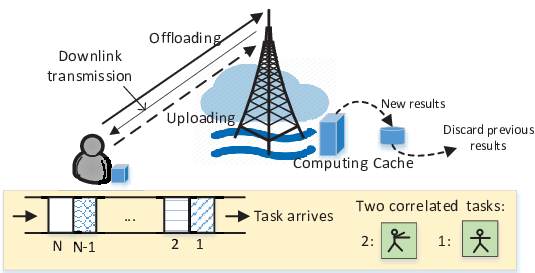
We consider a fog computing system consisting of one UT equipped with one single antenna, and one access point (AP) equipped with $M$ antennas, an edge server and cache facilities. During slot $i$, the UT solicits the nearby AP for computation task offloading. In this paper, we focus on a finite slotted-time horizon with each slot lasting $T$ seconds, denoted by $\mathcal{N}=\{1,\ldots,N\}$, over which sequential tasks featuring temporally correlated input data arrive at the UT as shown in Fig. 1. We assume that each task has to be executed by the end of the time slot. Since the computing results obtained at the current slot are also correlated with those at future slots, current task results can be cached at the AP to facilitate the future computation¹¹ 1 A typical example is matrix-vector multiplication of $\mbox{\boldmath{$y$}}_{i}=\mbox{\boldmath{$A$}}\mbox{\boldmath{$x$}}_{i}$, $i\in\mathcal{N}$, where $x_{i}$’s is the encoded task-input data. Supposing $\mbox{\boldmath{$x$}}_{i}=\mbox{\boldmath{$x$}}_{i-1}+\mbox{\boldmath{$\varepsilon$}}$ with a sparse error $\varepsilon$, the current computation can benefit from caching at slot $i-1$ by executing only $\varepsilon$ with much shorter input length.. Due to the extra overhead caused by caching (delay, energy, storage), it may not be optimal to cache all the execution results at the edge server. Therefore, we introduce the following variable $I_{i}$, $i\in\mathcal{N}$, to indicate whether the AP decides to cache the results at the end of slot $i$:

As a result, the workflow of the cache-enabled fog computing system in consideration can be described as follows. The UT offloads a proportion of the task to the AP while performing local computing for the rest of the task. If the AP decides not to cache the task results of the current slot, the UT just need to receive the execution results from the AP, otherwise the UT is also required to upload its local computing results to the AP at the end of the current slot. Since the AP is usually of sufficient communications resource. e.g., high transmitting power, we ignore the delay/energy caused by results downloading at the UT in the sequel.

In this section, we consider offline solution for problem (P1) by assuming that the predictable task-input length $\{L_{i}\}$ are perfectly known a priori at the AP. The offline solution thus serves as fundamental performance upper bound for all other online schemes that are designed for practical implementation. In this paper, we focus on a special case of $r=2$ (c.f. (2)). More general cases will be studied in our future work.

The major difficulty for solving (P1) lies in the binary variables $I_{i}$’s. To tackle this challenge, first, we equivalently formulate (7d) as $I_{i}(I_{i}-1)=0$, $\forall i\in\mathcal{N}$), and then transform the problem into a quadratically constrained quadratic program (QCQP) in terms of $\mbox{\boldmath{$I$}}=[I_{1},\ldots,I_{N}]^{T}$. Next, we convert the QCQP into a semi-definite programming (SDP) as follows. First, we define $\mbox{\boldmath{$F$}}^{\prime}=[(1-\tau_{2})\mbox{\boldmath{$F$}},\tfrac{1}{2}\mbox{\boldmath{$v$}};\tfrac{1}{2}\mbox{\boldmath{$v$}}^{T},0]$, where $\mbox{\boldmath{$F$}}=\sum\limits_{i=3}^{N}\tfrac{p_{i}L_{i}}{r_{i}^{\rm off}}\mbox{\boldmath{$G$}}_{i-2,i-1}$, $\mbox{\boldmath{$G$}}_{i-2,i-1}$ is a symmetric matrix with only $\mbox{\boldmath{$G$}}_{i-2,i-1}(i-2,i-1)$ and $\mbox{\boldmath{$G$}}_{i-2,i-1}(i-1,i-2)$ being $\tfrac{1}{2}$, $\mbox{\boldmath{$v$}}=(\tau_{1}-1)\sum\limits_{i=2}^{N}\tfrac{p_{i}L_{i}}{r_{i}^{\rm off}}\mbox{\boldmath{$e$}}_{i-1}+(\tau_{2}-1)\sum\limits_{i=3}^{N}\tfrac{p_{i}L_{i}}{r_{i}^{\rm off}}\mbox{\boldmath{$e$}}_{i-2}$, and $\mbox{\boldmath{$e$}}_{j}$ denotes a vector with only the $j$th element being $1$; $\mbox{\boldmath{$W$}}=[\mbox{\boldmath{$0$}}_{N\times N},\tfrac{1}{2}\mbox{\boldmath{$w$}};\tfrac{1}{2}\mbox{\boldmath{$w$}}^{T},0]$, where $\mbox{\boldmath{$w$}}=[\tfrac{p_{1}R_{1}}{r_{1}^{\rm up}},\ldots,\tfrac{p_{N}R_{N}}{r_{N}^{\rm up}}]^{T}$; $\mbox{\boldmath{$u$}}=[\tfrac{p_{1}}{r_{1}^{\rm off}},\ldots,\tfrac{p_{N}}{r_{N}^{\rm off}}]^{T}$, $\mbox{\boldmath{$G$}}^{\prime}=[(1-\tau_{2})\mbox{\boldmath{$G$}},\tfrac{1}{2}\mbox{\boldmath{$s$}};\tfrac{1}{2}\mbox{\boldmath{$s$}}^{T},0]$, where $\mbox{\boldmath{$G$}}=c_{\rm e}\sum\limits_{i=3}^{N}L_{i}\mbox{\boldmath{$G$}}_{i-2,i-1}$, and $\mbox{\boldmath{$s$}}=(\tau_{1}-1)c_{\rm e}\sum\limits_{i=2}^{N}L_{i}\mbox{\boldmath{$e$}}_{i-1}+(\tau_{2}-1)c_{\rm e}\sum\limits_{i=3}^{N}L_{i}\mbox{\boldmath{$e$}}_{i-2}$; $\mbox{\boldmath{$E$}}_{i}=[\mbox{\boldmath{$0$}}_{N\times N},\tfrac{1}{2}\mbox{\boldmath{$e$}}_{i};\tfrac{1}{2}\mbox{\boldmath{$e$}}_{i}^{T},0]$; and $\mbox{\boldmath{$U$}}_{i}=[\mathrm{diag}(\mbox{\boldmath{$e$}}_{i}),-\tfrac{1}{2}\mbox{\boldmath{$e$}}_{i};-\tfrac{1}{2}\mbox{\boldmath{$e$}}_{i}^{T},0]$. Next, we introduce $\mbox{\boldmath{$a$}}=[\mbox{\boldmath{$I$}};1]$ and $\mbox{\boldmath{$A$}}=\mbox{\boldmath{$a$}}\mbox{\boldmath{$a$}}^{T}$. Then, by relaxing the rank-one constraint for $A$ [11] and some manipulations, problem (P1) is recast into an SDP as shown in the following proposition.

In the previous section, we have provided an SDR-based offline solution under the ideal assumption that the random task-input length $L_{i}$’s is perfectly predicted without error. In this section, inspired by the offline solution, we propose a sliding-window based online scheme that applies to error sequence $\{\Delta L_{1},\ldots,\Delta L_{N}\}$ following arbitrary stochastic process [13].

Specifically, as stated in Section II, at any slot $i$, the exact task-input length is perfectly known up to the current slot, i.e., $\{L_{1},\ldots,L_{i}\}$, whereas only the predictable task-input length, i.e., $\hat{L}_{i+1},\ldots,\hat{L}_{N}$, is available for all future slots. First, we define a set $\mathcal{S}=\{1,\ldots,S\}$, where $S$ is the length of the sliding-window. Note that since the parameter $S$ balances between exploitation of the long-term prediction and accuracy of the algorithm, it is required to be carefully chosen in practice. Second, we focus on minimizing the weighted-sum energy over the span of the sliding-window from slot $i$, i.e., slots $\{i,\ldots,i+S-1\}$. Then, by specifying the parameters using their consecutive $S$-slot values from slot $i$³³ 3 When the last index of the sliding-window exceeds $N$, we substitute the (prediction) values of the parameters from slot $1$ to $S-1$ for those from slot $N+1$ to $N+S-1$., e.g., $\{L_{1}^{(i)},L_{2}^{(i)},\ldots,L_{S}^{(i)}\}=\{L_{i},\hat{L}_{i+1},\ldots,\hat{L}_{i+S-1}\}$, we sequentially solve the following problem for all the slots.

where $\mbox{\boldmath{$e$}}_{j}$, $j\in\mathcal{S}$, is similarly defined as in $\mathrm{(P1^{\prime})}$, and so are $\mbox{\boldmath{$E$}}_{j}$’s and $\mbox{\boldmath{$U$}}_{j}$’s through proper dimension modification. Next, by reconstructing $\mbox{\boldmath{$I$}}^{{\rm app}(i)}$ and $\mbox{\boldmath{$l$}}^{{\rm app}(i)}$ from the solution to $\mathrm{(P1\text{-}ol)}$, we attain the proposed online computation offloading policies $\{\tilde{l}_{i}\}$ and caching decisions $\{\tilde{I}_{i}\}$ by $\tilde{l}_{i}=l_{1}^{{\rm app}(i)}$ and $\tilde{I}_{i}=I_{1}^{{\rm app}(i)}$, $i\in\mathcal{N}$, respectively. The above procedure for the online scheme is summarized in Table I.

In this section, we verify the effectiveness of our proposed online computation offloading and caching scheme against theoretical performance upper bound and other benchmark schemes through numerical simulations. Specifically, ‘Lower-bound’ shows the optimal solution to $\mathrm{(P1^{\prime})}$ based on SDR, which is only achievable when the approximation is tight; ‘Random caching’ is obtained by setting $\{I_{i}\}$ as a $\tfrac{1}{2}$-Bernoulli process; ‘No caching’ refers to the results ignoring the correlation among task-input data; and “All caching” provides the case when $\{I_{i}=1\}$. At each slot, we consider Rayleigh fading channel models with the distance-dependent pathloss set as $-117$dB ($0.5$km) over transmission BWs of $B_{\rm off}=B_{\rm up}=2.5$MHz. The estimation of the task-input length follows a uniform distribution, denoted by $\hat{L}_{i}\sim\mathcal{U}[10^{5},10^{6}]$bits, $i\in\mathcal{N}$, and the profile of the associated task-output length is set as $R_{i}\sim\mathcal{U}[10^{5},10^{6}]$bits. Other parameters are set as follows unless otherwise specified: $M=3$; $\alpha_{1}=0.85$, $\alpha_{0}=0.15$; $\{\tau_{1}=\tfrac{1}{2},\tau_{2}=\tfrac{3}{4}\}$; $\{p_{i}=24\}$dBm; $f_{\rm loc}=800$MHz, $f_{\rm e}=2$GHz; $C_{\rm loc}=C_{\rm e}=10^{3}$ cycles/bit; and $\kappa_{\rm loc}=\kappa_{\rm e}=10^{-28}$. The results shown below are obtained by averaging over $500$-time realizations of the predication error sequence $\{\Delta L_{i}\}$, in which $\Delta L_{i}$’s is modelled as $i.i.d.$ Gaussian variables with zero mean and variance of $\sigma^{2}$.

Fig. 2 shows the average weighted-sum energy versus the computation deadline $T$ with $\sigma^{2}=10^{4}$. It is observed that the weighted-sum energy for all the schemes gradually goes down as the per-slot deadline gets extended, which is intuitively true, since the longer $T$ is, the higher the chances that more of the task-input bits can be executed locally within the deadline, which thus saves UT’s energy for task offloading. The approximate offline solution is also shown to approach the lower-bound SDR solution with negligible gap. Furthermore, the proposed online joint computation offloading and caching scheme outperforms all the other fixed-caching schemes, which corroborates the importance of computation caching in latency-critical scenarios.

Fig. 3 demonstrates the average weighted-sum energy versus the standard variance of the prediction error $\Delta L_{i}$’s. It is seen that our online algorithms under different deadline constraints are overall robust against a wide range of standard variance. In both cases of $T=0.3$ and $T=0.4$ seconds, the performance of the online scheme with a window length of $S=6$ is inferior to that with a window length of $S=4$ with noticeably larger gap in the more strict deadline constraint of $T=0.3$, which is due to the advantage of the short-size window in coping with uncertainties. Furthermore, the online algorithm with $S=6$ becomes worse off when $\sigma$ exceeds about $5\times 10^{4}$ ($7\times 10^{4}$) in the case of $T=.3$ ($T=.4$) seconds, since the effectiveness of the long-term prediction starts being compromised by the increasing estimation error.

This paper studied a one-UT one-AP fog computing system over a finite time-slotted horizon, in which each computation task was required to be executed by the end of the slot, and dynamic computation caching was allowed such that the AP could decide whether to cache the current task results for relieving its computation burden in the future. Under the assumption of three-slot correlation and imperfect estimation of the task-input bit-length, a joint computation offloading and caching optimization problem was formulated to minimize the long-term weighted-sum energy consumption of the UT and the AP. To tackle the challenging mixed-integer non-convex problem, we approximated the problem by an SDP, based on which an offline solution assuming perfect knowledge of task-input length was provided, while a sliding-window based online scheme was also developed to cater for unknown prediction error of the future task arrivals. By comparison with several benchmark schemes, the proposed online algorithm with short-size window demonstrated striking robustness against prediction error. In addition, the approximation was also shown to be near-optimal by numerical examples under practical settings.

References

- [1] R. Tandon and O. Simeone, “Harnessing cloud and edge synergies: toward an information theory of fog radio access networks,” IEEE Commun. Mag., vol. 54, no. 8, pp. 44–50, Aug. 2016.
- [2] Y. Y. Shih, W. H. Chung, A. C. Pang, T. C. Chiu, and H. Y. Wei, “Enabling low-latency applications in fog-radio access networks,” IEEE Netw., vol. 31, no. 1, pp. 52–58, Jan. 2017.
- [3] F. Wang, J. Xu, X. Wang, and S. Cui, “Joint offloading and computing optimization in wireless powered mobile-edge computing systems,” IEEE Trans. Wireless Commun., vol. 17, no. 3, pp. 1784–1797, Mar. 2018.
- [4] M. Chen, B. Liang, and M. Dong, “Multi-user multi-task offloading and resource allocation in mobile cloud systems,” IEEE Trans. Wireless Commun., vol. 17, no. 10, pp. 6790–6805, Oct. 2018.
- [5] Y. Mao, J. Zhang, and K. B. Letaief, “Dynamic computation offloading for mobile-edge computing with energy harvesting devices,” IEEE J. Sel. Areas Commun., vol. 34, no. 12, pp. 3590–3605, Dec. 2016.
- [6] E. Bastug, M. Bennis, and M. Debbah, “Living on the edge: The role of proactive caching in 5g wireless networks,” IEEE Commun. Mag., vol. 52, no. 8, pp. 82–89, Aug. 2014.
- [7] M. S. Elbamby, M. Bennis, and W. Saad, “Proactive edge computing in latency-constrained fog networks,” in Proc. European Conference on Networks and Communications (EuCNC), Oulu, Finland, Jun. 2017.
- [8] J. Xu, L. Chen, and P. Zhou, “Joint service caching and task offloading for mobile edge computing in dense networks,” in Proc. IEEE International Conference on Computer Communications (INFOCOM), Honolulu, HI, USA, Apr. 2018.
- [9] Y. Hao, M. Chen, L. Hu, M. S. Hossain, and A. Ghoneim, “Energy efficient task caching and offloading for mobile edge computing,” IEEE Access, vol. 6, pp. 11 365–11 373, Mar. 2018.
- [10] P. Mach and Z. Becvar, “Mobile edge computing: A survey on architecture and computation offloading,” IEEE Commun. Surveys Tuts., vol. 19, no. 3, pp. 1628–1656, third quart. 2017.
- [11] Z.-Q. Luo, W.-K. Ma, A. M.-C. So, Y. Ye, and S. Zhang, “Semidefinite relaxation of quadratic optimization problems,” IEEE Signal Process. Mag., vol. 27, no. 3, pp. 20–34, May 2010.
- [12] M. Grant and S. Boyd, “CVX: Matlab software for disciplined convex programming, version 2.1,” Mar. 2014. [Online]. Available: http://cvxr.com/cvx
- [13] K. Rahbar, J. Xu, and R. Zhang, “Real-time energy storage management for renewable integration in microgrid: An off-line optimization approach,” IEEE Trans. Smart Grid, vol. 6, no. 1, pp. 124–134, Jan. 2015.