Push-Pull Optimization of Quantum Controls
Abstract
Optimization of quantum controls to achieve a target process is centered around an objective function comparing the a realized process with the target. We propose an objective function that incorporates not only the target operator but also a set of its orthogonal operators, whose combined influences lead to an efficient exploration of the parameter space, faster convergence, and extraction of superior solutions. The push-pull optimization, as we call it, can be adopted in various quantum control scenarios. We describe adopting it to a gradient based and a variational-principle based approaches. Numerical analysis of quantum registers with up to seven qubits reveal significant benefits of the push-pull optimization. Finally, we describe applying the push-pull optimization to prepare a long-lived singlet-order in a two-qubit system using NMR techniques.
Keywords:
Optimal control theory, gradient optimization, variational approach, nuclear magnetic resonanceIntroduction: Optimal control theory finds applications in diverse fields such as finance, science, engineering, etc. Bryson 2018; Pontryagin 2018. Quantum optimal control has also gained significant attention over the last several years Werschnik and Gross 2007; Dong and Petersen 2010 and is routinely used in robust steering of quantum dynamics as in chemical kinetics Brumer and Shapiro 1989; Petzold and Zhu 1999, spectroscopy Tannor and Rice 1985; Zhu et al. 1998; Nielsen et al. 2007, quantum computing Palao and Kosloff 2002; Doria et al. 2011, and many more. Here we focus on optimization of quantum controls to either transfer from one state to another, henceforth called state control, or to realize a target unitary evolution, henceforth called gate control. Relevant numerical techniques fall into several categories including: stochastic-search methods such as strongly modulating pulses Fortunato et al. 2002; gradient based approaches such as gradient ascent pulse engineering (GRAPE) Khaneja et al. 2005; De Fouquieres et al. 2011 and gradient optimization of analytical control (GOAT) Machnes et al. 2018; variational-principle based Krotov optimization Krotov 2008; Maximov et al. 2008; Reich et al. 2012; truncated basis approach such as chopped random basis optimization (CRAB) Caneva et al. 2011; Sørensen et al. 2018; genetic algorithm enabled bang-bang controls Bhole et al. 2016; Khurana and Mahesh 2017; and machine learning based approaches Chen et al. 2013; Zhang et al. 2019. These control schemes have been implemented on various quantum architectures such as NMR Fortunato et al. 2002; Vandersypen and Chuang 2005; Nielsen et al. 2007; Bhole et al. 2016, NV centers Dolde et al. 2014, ion trap Singer et al. 2010, superconducting qubits Shim and Tahan 2016, magnetic resonance imaging Vinding et al. 2012, cold atoms Doria et al. 2011 etc.
An objective function evaluating the overlap of the realized process with the target process is at the core of an optimization algorithm and therefore should be chosen carefully Chakrabarti and Rabitz 2007; Pechen and Tannor 2011. Here we propose a hybrid objective function that not only depends on the target operator, but also on a set of orthogonal operators. One may think of control parameters being pulled by the target operator as well as pushed by the orthogonal operators. Accordingly, we refer to this method as Push-Pull Optimization of Quantum Controls (PPOQC). We describe adopting PPOQC for GRAPE and Krotov algorithms and demonstrate its superior convergence over the standard pull-only methods. We also experimentally demonstrate the efficacy of PPOQC in a NMR quantum testbed by preparing long-lived singlet-order.
The optimization problem: Consider a quantum system with an internal or fixed Hamiltonian and a set of control operators leading to the full time-dependent Hamiltonian
| (1) |
where control amplitudes are amenable to optimization.
The propagator for a control sequence of duration is
,
where is the Dyson time-ordering operator. The standard approach to simplify the propagator is via piecewise-constant control amplitudes with segments each of duration (see Fig. 1(a)). In this case, the overall propagator is of the form
, where
is the propagator for the th segment
and
.
Our task is to optimize the control sequence depending on the following two kinds of optimizations:
(i) Gate control (GC): Here the goal is to achieve an overall propagator (gate) that is independent of the initial state. This is realized by maximizing
the gate-fidelity
| (2) |
(ii) State control (SC): Here the goal is to drive a given initial state to a desired target state . This can be achieved by maximizing the state-fidelity
| (3) |
where .
In practice, hardware limitations impose bounds on the control parameters and therefore it is desirable to minimize the overall control resource . To this end, we use the performance function , where are penalty constants.

PPOQC: Be it gate control or state control, for a -dimensional target operator, we can efficiently setup orthogonal operators via Gram-Schmidt orthogonalization procedure Shankar 2012. The target operator pulls the control-sequence towards itself, whereas the orthogonal operators push it away from them (see Fig. 1(b)). We define the push fidelities as
| (4) |
where and are orthogonal operators such that and . Of course, increases exponentially with the system size, but as we shall see later, a small subset of orthogonal operators can bring about a substantial advantage. Also, note that for a given target operator, the set of orthogonal operators is not unique and can be generated randomly and efficiently in every iteration. We define the push-pull performance function
| (5) |
where is the push weight. In the following, we describe incorporating PPOQC into two popular optimal quantum control methods.
GRAPE optimization: Being a gradient based approach, it involves an efficient calculation of the maximum-ascent direction Khaneja et al. 2005. While it is sensitive to the initial guess and looks for a local optimum, it is nevertheless simple, powerful, and popular. The algorithm iteratively updates control parameters in the direction of gradient :
| (6) |
where denotes iteration number, and Khaneja et al. 2005. Collective updates after iteration on all the segments with a suitable step size , proceeds with monotonic convergence.
Push-pull GRAPE (PP-GRAPE): Using Eq. 5 we recast the gradients as
| (7) |
and the update rule as . The revised gradients form the basis of PP-GRAPE.
Krotov optimization: Based on variational-principle, this method aims for the global optimum Krotov 1995. Here the performance function is maximized with the help of an appropriate Lagrange multiplier . One sets up a Lagrangian of the form Nielsen et al. 2007,
| (8) |
where the first two terms are same as the performance function , and looks for a stationary point satisfying . The second differential equation leads to , and the last differential equation constrains evolution according to the Schrödinger equation .
At every iteration , the Krotov algorithm evaluates the control sequence as well as its co-sequence . Starting with a random guess , forward propagation of the sequence gives and backward propagation of the co-sequence from the boundary leads to . Specifically,
| (9) |
Here , , and is a positive constant that ensures the positivity of fidelity. Back propagating the co-sequence, we obtain
| (10) |
where . Now the sequence is updated according to
| (11) |
and propagator is evaluated. Iterating the last two steps delivers propagators . The terminal Lagrange multiplier is evaluated using the Eq. 9. To setup the co-sequence we first evaluate the terminal control using
| (12) |
with . The Lagrange multiplier is now evaluated by back-propagating with the updated amplitude . Iterating the last two steps updates the whole co-sequence . The algorithm is continued until the desired fidelity is reached.
Push-pull Krotov (PP-Krotov): Here we use additional co-sequences corresponding to orthogonal operators or . Terminal Lagrange multipliers are obtained using similar equations as in Eq. 9:
| (13) |
The intermediate Lagrange multipliers are evaluated by back-propagating in a similar way as described in Eq. 10, but by replacing the target operator with orthogonal operator (or ). Revised update rule is
| (14) | |||||
where and is the push weight as in Eq. 5. We now proceed to numerically analyze PPOQC performance.
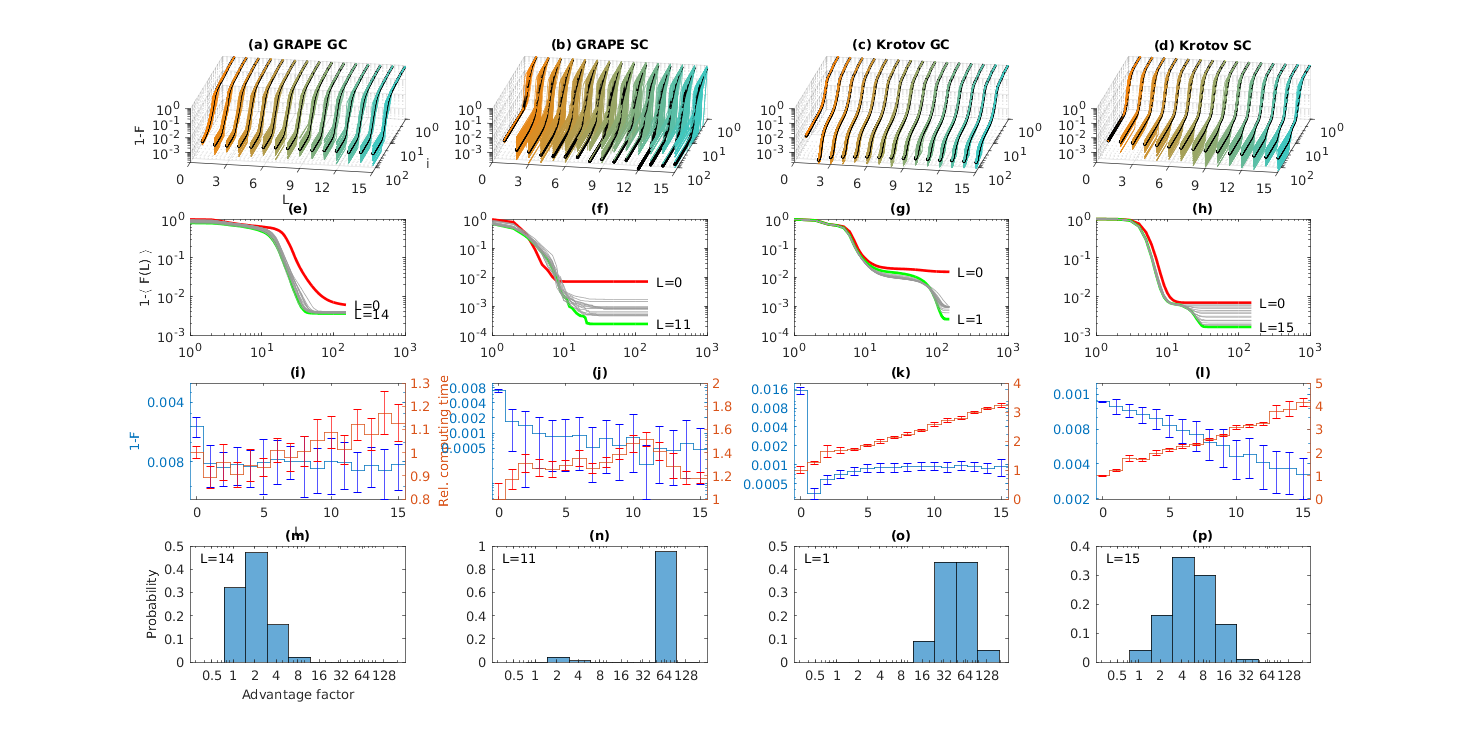
Numerical analysis: Results of PPOQC analysis in a model two-qubit Ising-coupled system are summarized in Fig. 2. For GC, we use CNOT gate as the target, while for SC, the task is a transfer from state to singlet state . In each case, we use a fixed set of one hundred random guess-sequences. PP-GRAPE and PP-Krotov algorithms were run for various sizes of orthogonal sets ( with push weight ) and compared with the pull-only () results (Fig. 2(a-d)). PPOQC outperformed the pull-only algorithms in terms of the mean final fidelity in all the cases (Fig. 2 (e-h)). More importantly, while the pull-only fidelities tend to saturate by settling into local minima, the push-pull trials appeared to explore larger parameter space and thereby extracted solutions with better fidelities. While the computational time for PP-GRAPE is weakly dependent on , we find a slow but linear increase in the case of PP-Krotov (Fig. 2 (i-l)). To quantify the advantage of PPOQC over the standard algorithms, we define the advantage factor , where corresponds to the one with maximum mean of final-fidelity (Fig. 2 (m-p)). In all the cases PPOQC () resulted in superior convergences than the standard pull-only () algorithms. In particular, PP-Grape SC and PP-Krotov GC reached advantage factors up to 64, while PP-Krotov SC reached up to 16. Only in PP-Grape GC, the advantage factor was modest 2.

To analyze the performance of PPOQC in larger systems, we implement Quantum Fourier Transform (QFT), which is central to several important quantum algorithms Nielsen et al. 2007. We implement the entire -qubit QFT circuit, consisting of local and conditional gates, into a single PP-Krotov GC sequence. The results, with registers up to seven qubits, shown in Fig. 3 assure that PPOQC advantage persists even in larger systems. Further discussions and numerical analysis are provided in supplemental materials. In the following, we switch to an experimental implementation of PPOQC pulse-sequence.

NMR experiments: We now study the efficacy of PPOQC via an important application in NMR spectroscopy, i.e., preparation of a long-lived state (LLS). Carravetta et al. had demonstrated that the singlet-order of a homonuclear spin-pair outlives the usual life-times imposed by spin-lattice relaxation time constant () Carravetta et al. 2004; Carravetta and Levitt 2004. Prompted by numerous applications in spectroscopy and imaging, several efficient ways of preparing LLS have been explored Pileio 2017. In the following, we utilize PP-Krotov SC optimization for this purpose.
We prepare LLS on two protons of 2,3,6-trichlorophenol (TCP; see Fig. 4 (a)). Sample consists of 7 mg of TCP dissolved in 0.6 ml of deuterated dimethyl sulfoxide. The experiments are carried out on a Bruker 500 MHz NMR spectrometer at an ambient temperature of 300 K. Standard NMR spectrum of TCP shown in Fig. 4 (a) indicates resonance offset frequencies to be Hz and the scalar coupling constant Hz. The internal Hamiltonian of the system, in a frame rotating about the direction of the Zeeman field at an average Larmor frequency is
where and are the -components of the spin angular momentum operators and respectively.
The thermal equilibrium state at high-field and high-temperature approximation is of the form (up to an identity term representing the background population). The goal is to design an RF sequence introducing a time-dependent Hamiltonian
that efficiently transfers into zero-quantum singlet-triplet order . Under an RF spin-lock the triplet order decays rapidly while the singlet order remains long-lived. The PP-Krotov SC pulse-sequence shown in Fig. 4 (b) consists of 1000 segments in a total duration of 45 ms, which is 30% shorter than the standard sequence that requires ms Carravetta and Levitt 2004. The fidelity profile shown in Fig. 4 (c) indicates the robustness of the sequence against RF inhomogeneity distribution with an average final fidelity above 95%. The LLS spectrum shown in Fig. 4(a) is the characteristic of the singlet state . Fig. 4 (d) shows the experimental results of LLS storage under 1 kHz WALTZ-16 spin-lock. It confirms the long life-time of about 24.5 s or about 4.5 times and measured by inversion recovery experiments. A comparison with the standard method (as in ref. Carravetta and Levitt 2004) revealed 27% higher singlet order, further indicating the superiority of the PP-Krotov SC sequence.
Summary: At the heart of optimization algorithms lies a performance function that evaluates a process in relation to a target. Using a hybrid objective function that simultaneously takes into account a given target operator as well as a set of orthogonal operators we devised the push-pull optimization of quantum controls. Combined influences of these operators not only results in a faster convergence of the optimization algorithm, but also effects a better exploration of the parameter space and thereby generates better solutions. Although the orthogonal set grows exponentially with the system size, it is not necessary to include an exhaustive set. Even a small set of orthogonal operators, generated randomly during the iterations, can bring about a significant improvement in convergence. While the push-pull approach can be implemented in a wide variety of quantum control routines, we described adopting it into a gradient based as well as a variational-principle based optimizations. We observed considerable improvements in the convergence rates, without overburdening computational costs. The numerical analysis with up to seven qubits confirmed that push-pull method retained superiority even in larger systems. Finally, using NMR methods, we experimentally verified the robustness of a push-pull Krotov control sequence preparing a long-lived singlet order. Further work in this direction includes adaptive push-weights, optimizing the functional forms of orthogonal gradients, generalization to open quantum controls, and so on.
Acknowledgments: Discussions with Sudheer Kumar, Deepak Khurana, Soham Pal, Gaurav Bhole, Dr. Hemant Katiyar, and Dr. Pranay Goel are gratefully acknowledged. This work was partly supported by DST/SJF/PSA-03/2012-13 and CSIR 03(1345)/16/EMR-II.
References
- Bryson (2018) A. E. Bryson, Applied optimal control: optimization, estimation and control (Routledge, 2018).
- Pontryagin (2018) L. S. Pontryagin, Mathematical theory of optimal processes (Routledge, 2018).
- Werschnik and Gross (2007) J. Werschnik and E. Gross, Journal of Physics B: Atomic, Molecular and Optical Physics 40, R175 (2007).
- Dong and Petersen (2010) D. Dong and I. R. Petersen, IET Control Theory & Applications 4, 2651 (2010).
- Brumer and Shapiro (1989) P. Brumer and M. Shapiro, Accounts of Chemical Research 22, 407 (1989).
- Petzold and Zhu (1999) L. Petzold and W. Zhu, AIChE journal 45, 869 (1999).
- Tannor and Rice (1985) D. J. Tannor and S. A. Rice, The Journal of chemical physics 83, 5013 (1985).
- Zhu et al. (1998) W. Zhu, J. Botina, and H. Rabitz, The Journal of Chemical Physics 108, 1953 (1998).
- Nielsen et al. (2007) N. C. Nielsen, C. Kehlet, S. J. Glaser, and N. Khaneja, eMagRes (2007).
- Palao and Kosloff (2002) J. P. Palao and R. Kosloff, Physical review letters 89, 188301 (2002).
- Doria et al. (2011) P. Doria, T. Calarco, and S. Montangero, Physical review letters 106, 190501 (2011).
- Fortunato et al. (2002) E. M. Fortunato, M. A. Pravia, N. Boulant, G. Teklemariam, T. F. Havel, and D. G. Cory, The Journal of chemical physics 116, 7599 (2002).
- Khaneja et al. (2005) N. Khaneja, T. Reiss, C. Kehlet, T. Schulte-Herbrüggen, and S. J. Glaser, Journal of magnetic resonance 172, 296 (2005).
- De Fouquieres et al. (2011) P. De Fouquieres, S. Schirmer, S. Glaser, and I. Kuprov, Journal of Magnetic Resonance 212, 412 (2011).
- Machnes et al. (2018) S. Machnes, E. Assémat, D. Tannor, and F. K. Wilhelm, Physical review letters 120, 150401 (2018).
- Krotov (2008) V. Krotov, in Doklady Mathematics, Vol. 78 (Springer, 2008) pp. 949–952.
- Maximov et al. (2008) I. I. Maximov, Z. Tošner, and N. C. Nielsen, The Journal of Chemical Physics 128, 05B609 (2008).
- Reich et al. (2012) D. M. Reich, M. Ndong, and C. P. Koch, The Journal of chemical physics 136, 104103 (2012).
- Caneva et al. (2011) T. Caneva, T. Calarco, and S. Montangero, Physical Review A 84, 022326 (2011).
- Sørensen et al. (2018) J. Sørensen, M. Aranburu, T. Heinzel, and J. Sherson, Physical Review A 98, 022119 (2018).
- Bhole et al. (2016) G. Bhole, V. Anjusha, and T. Mahesh, Physical Review A 93, 042339 (2016).
- Khurana and Mahesh (2017) D. Khurana and T. Mahesh, Journal of Magnetic Resonance 284, 8 (2017).
- Chen et al. (2013) C. Chen, D. Dong, H.-X. Li, J. Chu, and T.-J. Tarn, IEEE transactions on neural networks and learning systems 25, 920 (2013).
- Zhang et al. (2019) X.-M. Zhang, Z. Wei, R. Asad, X.-C. Yang, and X. Wang, arXiv preprint arXiv:1902.02157 (2019).
- Vandersypen and Chuang (2005) L. M. Vandersypen and I. L. Chuang, Reviews of modern physics 76, 1037 (2005).
- Dolde et al. (2014) F. Dolde, V. Bergholm, Y. Wang, I. Jakobi, B. Naydenov, S. Pezzagna, J. Meijer, F. Jelezko, P. Neumann, T. Schulte-Herbrüggen, et al., Nature communications 5, 3371 (2014).
- Singer et al. (2010) K. Singer, U. Poschinger, M. Murphy, P. Ivanov, F. Ziesel, T. Calarco, and F. Schmidt-Kaler, Reviews of Modern Physics 82, 2609 (2010).
- Shim and Tahan (2016) Y.-P. Shim and C. Tahan, Nature communications 7, 11059 (2016).
- Vinding et al. (2012) M. S. Vinding, I. I. Maximov, Z. Tošner, and N. C. Nielsen, The Journal of chemical physics 137, 054203 (2012).
- Chakrabarti and Rabitz (2007) R. Chakrabarti and H. Rabitz, International Reviews in Physical Chemistry 26, 671 (2007).
- Pechen and Tannor (2011) A. N. Pechen and D. J. Tannor, Physical review letters 106, 120402 (2011).
- Shankar (2012) R. Shankar, Principles of quantum mechanics (Springer Science & Business Media, 2012).
- Krotov (1995) V. Krotov, Global methods in optimal control theory, Vol. 195 (CRC Press, 1995).
- Carravetta et al. (2004) M. Carravetta, O. G. Johannessen, and M. H. Levitt, Physical review letters 92, 153003 (2004).
- Carravetta and Levitt (2004) M. Carravetta and M. H. Levitt, Journal of the American Chemical Society 126, 6228 (2004).
- Pileio (2017) G. Pileio, Progress in nuclear magnetic resonance spectroscopy 98, 1 (2017).
Supplemental information
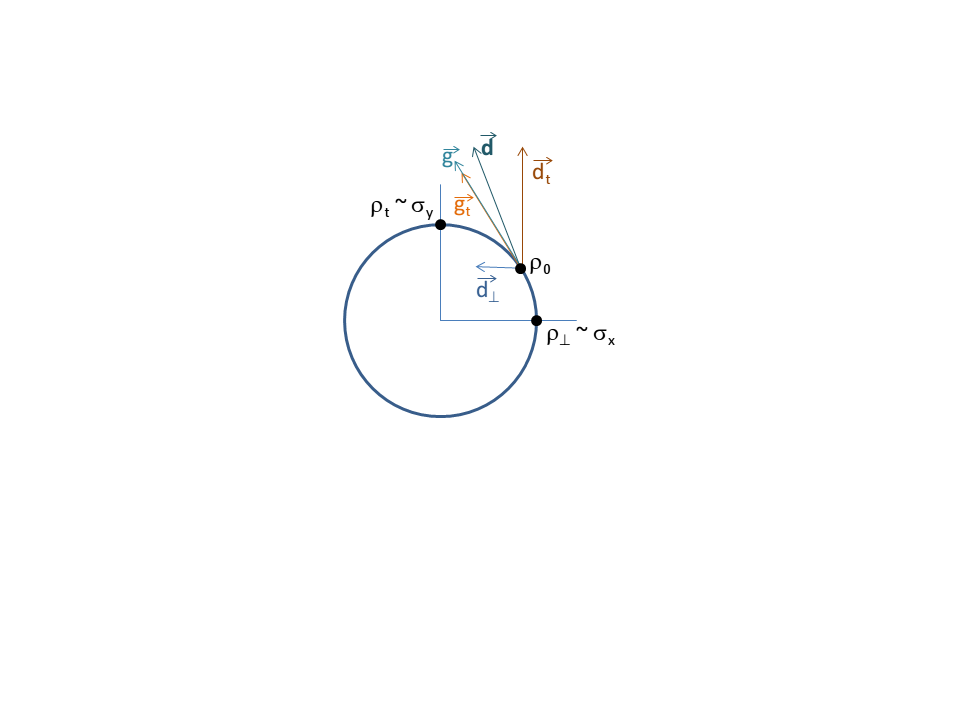
A naive model: Consider a single qubit state control problem with target being the pure state and its orthogonal state being . Consider an instantaneous state . To simplify the picture, we consider the dynamics in xy-plane of the Bloch sphere by fixing (see Fig. 5). In the pull-only scenario, the pull direction is along that is parallel to -axis. Since the dynamics is constrained on the unit circle, the corresponding gradient is the tangential component of . In the push-pull case, we also have a direction that is along -axis so that the net push-pull direction is along . Now the corresponding tangential component has a magnitude greater than since is the resultant of nonparallel vectors. Of course, this simple model does not capture the entire picture, neither does it fully grasp the push-roles of orthogonal operators. Nevertheless, the stronger gradients in the push-pull scenario hint about its faster convergence.
Push-weight: Fig. 6 displays infidelities of PP-GRAPE as well as PP-Krotov algorithms versus the push-weight . We notice that, on the positive side, the infidelity is generally superior to the pull-only algorithm (). In each case, there exists an optimal push-weight roughly in the range at which the PPOQC works best. It is interesting to see that some negative regions also display superior performances.
Rapid parameter search in push-pull approach: To gain insight into the superiority of push-pull over pull-only approach, we observed how the gradients evolve over time. Fig. 7 displays the evolution of gradients versus control amplitudes over several iterations. The simulations are carried out for a two-qubit CNOT gate with both pull-only and push-pull GRAPE algorithms. Push-pull algorithm ultimately converged to a better fidelity (0.993) than the pull-only algorithm (0.981). Notice that the push-pull gradients show more rapid changes than the pull-only algorithm, indicating a more robust parameter search in action. This behavior appears to be the crucial factor for the faster convergence of the push-pull approach.
