跳到论文正文
W Papers独立论文阅读器 arXiv:1908.06276 论文正文 计算阅读时间 · 0%
引用这篇论文根据当前论文元数据生成,正式投稿前建议核对。


License: arXiv.org perpetual non-exclusive license
arXiv:1908.06276v3 [math.DG] 27 Oct 2020

Stacking disorder in periodic minimal surfacesThanks: H. Chen is supported by Individual Research Grant from Deutsche Forschungsgemeinschaft within the project “Defects in Triply Periodic Minimal Surfaces”, Projektnummer 398759432. M. Traizet is supported by the ANR project Min-Max (ANR-19-CE40-0014)

Hao Chen ChenGeorg-August-Universität Göttingen, Institut für Numerische und Angewandte Mathematik Email address: h.chen@math.uni-goettingen.de and Martin Traizet TraizetInstitut Denis Poisson, CNRS UMR 7350, Faculté des Sciences et Techniques, Université de Tours Email address: martin.traizet@lmpt.univ-tours.fr
Date: August 11, 2026
Abstract.

We construct 1-parameter families of non-periodic embedded minimal surfaces of infinite genus in T×ℝT\times\mathbb{R}, where TT denotes a flat 2-tori. Each of our families converges to a foliation of T×ℝT\times\mathbb{R} by TT. These surfaces then lift to minimal surfaces in ℝ3\mathbb{R}^{3} that are periodic in horizontal directions but not periodic in the vertical direction. In the language of crystallography, our construction can be interpreted as disordered stacking of layers of periodically arranged catenoid necks. Limit positions of the necks are governed by equations that appear, surprisingly, in recent studies on the Mean Field Equation and the Painlevé VI Equation. This helps us to obtain a rich variety of disordered minimal surfaces. Our work is motivated by experimental observations of twinning defects in periodic minimal surfaces, which we reproduce as special cases of stacking disorder.

Key words and phrases: 
minimal surfaces
2010 Mathematics Subject Classification
Primary 53A10

1. Introduction

1.1. Background

Triply periodic minimal surfaces (TPMSs) is a topic of trans-disciplinary interest. On the one hand, the mathematical notion has been employed to model many structures in nature (e.g. biological membrane) and in laboratory (e.g. lyotropic liquid crystals); we refer the readers to the book [HBL+96] for more information. On the other hand, natural scientists have been contributing with important mathematical discoveries, many long precede the rigorous mathematical treatment. Examples include the famous gyroid discovered in [Sch70] and proved in [GBW96], as well as its deformations discovered in [FHL93, FH99] and recently proved in [Che19a].

The current paper is another example in which mathematics is inspired by natural sciences. In [HXBC11], mesoporous crystals exhibiting the structure of Schwarz’ D surface are synthesized. Remarkably, a twinning structure, which looks like two copies of Schwarz’ D surface glued along a reflection plane, is observed. In other word, the periodicity is broken in the direction orthogonal to the reflection plane. Thereafter, many other crystal defects are experimentally observed in more TPMS structures, leading to a growing demand of mathematical understanding.

Recently, the first named author [Che19b] responded to this demand with numerical experiments in Surface Evolver [Bra92]. More specifically, periodic twinning defects are numerically introduced into rPD surfaces (see Figure 1) and the gyroid. Success of these experiments provide strong evidences for the existence of single twinning defects.

Moreover, he also became aware of the node-opening techniques developed by the second named author [Tra02]. The idea is to glue catenoid necks among horizontal planes. When the planes are infinitesimally close, the necks degenerate to singular points termed nodes. It is proved that, if the limit positions of the nodes satisfy a balancing condition and a non-degeneracy condition, then it is possible to push the planes a little bit away from each other, giving a 1-parameter family of minimal surfaces along the way. The technique has been used to construct TPMSs [Tra08] by gluing necks among finitely many flat tori, and non-periodic minimal surfaces with infinitely many planar ends [MT12] by gluing necks among infinitely many Riemann spheres.

In this paper, we combine the techniques in [Tra08] and [MT12] to glue necks among infinitely many flat tori. Then each balanced and non-degenerate arrangement of nodes gives rise to a 1-parameter families of minimal surfaces. Seen in T×ℝT\times\mathbb{R}, each of these family converges to a foliation of T×ℝT\times\mathbb{R} by TT. Seen in ℝ3\mathbb{R}^{3}, the minimal surfaces are periodic in two independent horizontal directions but not periodic in any other independent direction.

Our motivation is to rigorously construct twinning defects, but the examples produced by our construction is far richer. In the language of crystallography, our construction can be seen as stacking layers of periodically arranged catenoid necks. In the case that TT is the 60-degree torus, for example, we will see that any bi-infinite sequence of 5 stacking patterns gives arise to a 1-parameter family of minimal surfaces. These are then uncountably many families. In particular, a twinning defect arises from a stacking fault, which is not periodic but still quite ordered from a physics point of view. But most of our examples does not exhibit any order, hence should be considered as stacking disorders.

Back to the twinning, experiments and simulations have shown that TPMSs with twinning defects decay exponentially to the standard TPMSs. We will provide mathematical proof to this physics phenomenon, hence finally justify the term “TPMS twinning”. More specifically, we will prove that if a configuration is eventually periodic, then the corresponding minimal surface is asymptotic to a TPMS. The proof uses weighted Banach space as in [Tra13].

Our construction uses Implicit Function Theorem, hence only works near the degenerate limit of foliations, which is not physically plausible. However, physicists have proposed formation mechanisms for TPMSs in nature and in laboratory (e.g. [CF97, MBF94, CCM+06, TBC+15]) that are very similar to node-opening, some even with experiment evidences. Hence we may hope that some of the minimal surfaces constructed in this paper, including those with stacking disorders, would be one day observed in laboratory.
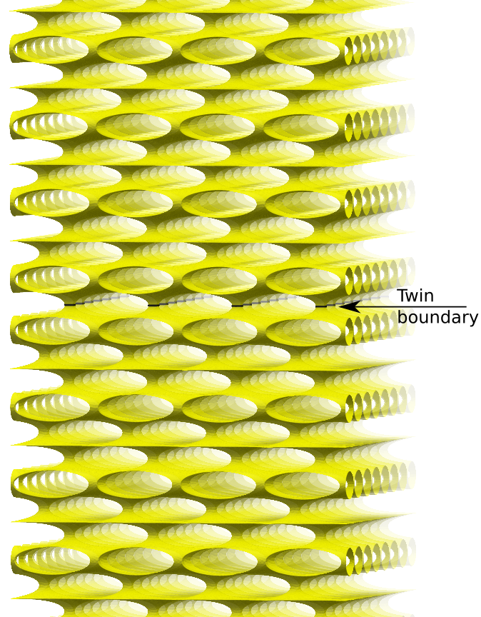
Refer to caption
Figure 1. Twinning defects in an rPD surface near the catenoid limit, as described in Example 5. This is actually an approximation by a TPMS with large vertical period. The surface has a horizontal symmetry plane in the middle. The image was computed in Surface Evolver [Bra92] using the procedure in [Che19b].

1.2. Mathematical setting

A doubly periodic minimal surface (DPMS) MM is invariant by two independent translations, which we may assume to be horizontal. Let Γ\Gamma be the two-dimensional lattice generated by these translations, then MM projects to a minimal surface M/ΓM/\Gamma in ℝ3/Γ=T×ℝ\mathbb{R}^{3}/\Gamma=T\times\mathbb{R}, where T=ℝ2/ΓT=\mathbb{R}^{2}/\Gamma denotes a flat 2-torus. Immediate examples of infinite genus are given by triply periodic minimal surfaces (TPMSs), if one ignores one of their three periods. Motivated by experimental observations mentioned above, we are particularly interested in non-periodic DPMS with infinite genus.

A flat torus in T×ℝT\times\mathbb{R} is horizontal if it has the form T×{h}T\times\{h\} for some h∈ℝh\in\mathbb{R}; then hh is called the height of the torus. Informally speaking, we construct minimal surfaces that look like infinitely many horizontal flat tori in T×ℝT\times\mathbb{R}, ordered by increasing height, with one catenoid neck between each adjacent pair. The tori are then labeled by k∈ℤk\in\mathbb{Z} in the order of height. The catenoid necks are also labeled by k∈ℤk\in\mathbb{Z}, such that the kk-th neck is between the kk-th and the (k+1)(k+1)-th tori.

Remark 1.1.

Our construction can, in principle, handle finitely many necks between each adjacent pair of tori. But in view of the immediate interest from material sciences, we will only glue one catenoid neck between each adjacent tori. This also eases the notations and facilitates the proofs, but still produces a rich variety of examples.

More formally, we say that a minimal surfaces M∈T×ℝM\in T\times\mathbb{R} is stacked if there is an increasing sequence of real numbers (hk)k∈ℤ(h_{k})_{k\in\mathbb{Z}} satisfying

  • •

    M∩(T×{hk})M\cap(T\times\{h_{k}\}) has a single connected component that projects to a null-homotopic smooth simple closed curve in TT;

  • •

    M∩(T×(hk,hk+1))M\cap(T\times(h_{k},h_{k+1})) is homeomorphic to TT with two disks removed.

Then the kk-th neck can be interpreted as an annular neighborhood of M∩(T×{hk})M\cap(T\times\{h_{k}\}).

Remark 1.2.

The term “stacked” is borrowed from crystallography. Closed-packed structures are often described as a result of stacking layers of periodically arranged atoms, one on top of another. Analogously, a stacked minimal surface can be seen as obtained by stacking layers of periodically arranged catenoid necks.

We intend to construct 1-parameter families MtM_{t}, t>0t>0, of stacked minimal surfaces such that, in the limit t→0t\to 0, every neck converges to a catenoid after suitable rescaling. If we rescale to keep the size of the torus, then MtM_{t} will converge to a foliation of T×ℝT\times\mathbb{R} by TT, and necks converge to singular points, which we call nodes.

1.3. Definitions and main result

Definition 1.1.

A node configuration is a sequence 𝒑=(pk)k∈ℤ\bm{p}=(p_{k})_{k\in\mathbb{Z}} such that pk∈Tp_{k}\in T for all k∈ℤk\in\mathbb{Z}.

We use pkp_{k} to prescribe the limit position of the kk-th node, and assume that

Hypothesis 1.2 (Uniform separation).

There exists a constant ϱ>0\varrho>0 such that pkp_{k} and pℓp_{\ell} are at least at distance ϱ\varrho apart whenever |k−ℓ|=1|k-\ell|=1.

Assume that 2​ω1=12\omega_{1}=1 and 2​ω2=τ2\omega_{2}=\tau generate the lattice Γ\Gamma, so T=Tτ=ℂ/(ℤ+τ​ℤ)T=T_{\tau}=\mathbb{C}/(\mathbb{Z}+\tau\mathbb{Z}). Without loss of generality, we also assume that Im⁡τ>0\operatorname{Im}\tau>0. Then for p∈Tp\in T, we use x⁡(p,τ)x(p;\tau) and y⁡(p,τ)y(p;\tau) to denote its coordinates in the basis 11 and τ\tau, and define the function

ξ⁡(p,τ)=x⁡(p,τ)​η1​(τ)+y⁡(p,τ)​η2​(τ),\xi(p;\tau)=x(p;\tau)\eta_{1}(\tau)+y(p;\tau)\eta_{2}(\tau),

where ηi​(τ)=ζ⁡(z+2​ωi,τ)−ζ⁡(z,τ)=2​ζ​(ωi,τ)\eta_{i}(\tau)=\zeta(z+2\omega_{i};\tau)-\zeta(z;\tau)=2\zeta(\omega_{i};\tau) for i=1,2i=1,2, and

ζ⁡(z,τ)=1z​∑0≠u∈ℤ+τ​ℤ(1z−u+1u+zu2)\zeta(z;\tau)=\frac{1}{z}\sum_{0\neq u\in\mathbb{Z}+\tau\mathbb{Z}}\Big(\frac{1}{z-u}+\frac{1}{u}+\frac{z}{u^{2}}\Big)

is the Weierstrass zeta function associated to Γ\Gamma.

The following definitions are borrowed from [Tra08] and [MT12]. Given a node configuration 𝒑\bm{p}, the force FkF_{k} exerted on the node pkp_{k} by other nodes is

(1) Fk:=ζ⁡(pk+1−pk,τ)+ζ⁡(pk−1−pk,τ)+2​ξ​(pk,τ)−ξ⁡(pk+1,τ)−ξ⁡(pk−1,τ)F_{k}:=\zeta(p_{k+1}-p_{k};\tau)+\zeta(p_{k-1}-p_{k};\tau)+2\xi(p_{k};\tau)-\xi(p_{k+1};\tau)-\xi(p_{k-1};\tau)
Definition 1.3.

A node configuration is said to be balanced if Fk=0F_{k}=0 for all k∈ℤk\in\mathbb{Z}.

Since our construction uses the Implicit Function Theorem, we need the differential of the force to be invertible in some sense. As explained in [MT12], (pk)(p_{k}) is not the right parameter to formulate non-degeneracy and one needs to introduce the sequence 𝒒=(qk)\bm{q}=(q_{k}) defined by

qk=pk−pk−1.q_{k}=p_{k}-p_{k-1}.

Note that the uniform separation hypothesis can be reformulated as (qk)(q_{k}) being bounded away from 00. From now on, we use the term “configuration” for the infinite sequence (qk)(q_{k}).

Under the new variables, (1) becomes

Fk:=ζ⁡(qk+1,τ)−ζ⁡(qk,τ)+ξ⁡(qk,τ)−ξ⁡(qk+1,τ)=Gk+1−Gk.F_{k}:=\zeta(q_{k+1};\tau)-\zeta(q_{k};\tau)+\xi(q_{k};\tau)-\xi(q_{k+1};\tau)=G_{k+1}-G_{k}.

where

Gk=G⁡(qk,τ)=ζ⁡(qk,τ)−ξ⁡(qk,τ).G_{k}=G(q_{k};\tau)=\zeta(q_{k};\tau)-\xi(q_{k};\tau).

A configuration is then balanced if (Gk)(G_{k}) is a constant sequence, i.e. Gk=G0G_{k}=G_{0} for all k∈ℤk\in\mathbb{Z}.

Definition 1.4.

A configuration is said to be non-degenerate if the differential of (Gk)k∈ℤ(G_{k})_{k\in\mathbb{Z}} with respect to (qk)k∈ℤ(q_{k})_{k\in\mathbb{Z}}, as a map from ℓ∞\ell^{\infty} to itself, is an isomorphism.

Note that G⁡(q,τ)G(q;\tau) is periodic in qq but not meromorphic. The function G⁡(q,τ)G(q;\tau) is called the Hecke form in [Lan95]. It was proved by Hecke [Hec27] that, if q=(k1+k2​τ)/Nq=(k_{1}+k_{2}\tau)/N with gcd⁡(k1,k2,N)=1\gcd(k_{1},k_{2},N)=1, then G⁡(q,τ)G(q;\tau) is a modular form of weight 11 with respect to the congruence group Γ⁡(N)\Gamma(N). Recently, the Hecke form gained popularity for its importance in the study of PDEs, including the Mean Field Equation, the Painlevé VI Equation, and the (generalized) Lamé Equation; see [Lin16] for a survey. We will exploit some of the recent results [LW10, CKLW18, BE16] in our construction.

Now we are ready to state our main theorems

Theorem 1.5.

If a configuration 𝐪\bm{q} is balanced, non-degenerate, and satisfies the uniform separation hypothesis, then there exists in T×ℝT\times\mathbb{R} a 1-parameter family (Mt)0<t<ϵ(M_{t})_{0<t<\epsilon} of embedded stacked minimal surfaces which, in the limit t→0t\to 0, converges to a foliation of T×ℝT\times\mathbb{R} by TT. Moreover, the necks have asymptotically catenoidal shape and their limiting positions in TT are prescribed by 𝐩\bm{p}.

Theorem 1.6.

Let 𝐪\bm{q} and 𝐪′\bm{q}^{\prime} be two balanced and non-degenerate configurations that satisfy the uniform separation hypothesis. Assume that (qk)(q_{k}) is periodic (in the sense qk+N=qkq_{k+N}=q_{k}) and qk′=qkq^{\prime}_{k}=q_{k} for all k≥0k\geq 0. Let (Mt)(M_{t}) and (Mt′)(M^{\prime}_{t}) denote the corresponding 1-parameter families of minimal surfaces. Then MtM_{t} is a TPMS and Mt′M^{\prime}_{t} is asymptotic to a translation of MtM_{t} as x3→∞x_{3}\to\infty.

The paper is organized by increasing technicality. After reviewing some examples in Section 2, we prove our main theorems in Section 3 and Section 4, respectively. Technical ingredients of the proofs are delayed to later sections. In Section 5 we prove the existence and smooth dependence on parameters of a holomorphic 1-form ω\omega that we used in the Weierstrass data in Section 3. In Section 6, we study the asymptotic behavior of ω\omega and other parameters, which is crucial for proving the TPMS asymptotic behavior in Section 4.

2. Examples

Given an infinite sequence of planes, if only one node is opened between each adjacent pair, the result is necessarily a Riemann minimal example [MT12]. We now show that opening nodes among flat tori is a sharp contrast. Although we only open one node between each adjacent pair of tori, we still obtain a rich variety of balanced configurations. We produce configurations using the following

Proposition 2.1.

Let q~0,q~1,⋯,q~n−1\widetilde{q}_{0},\widetilde{q}_{1},\cdots,\widetilde{q}_{n-1} be nn solutions of the equation

(2) G⁡(q,τ)=CG(q;\tau)=C

for the same complex constant CC. Assume that the differential of GG with respect to qq at q~k\widetilde{q}_{k}, as a function from ℝ2\mathbb{R}^{2} to ℝ2\mathbb{R}^{2}, is non-singular for each kk. Then any bi-infinite sequence (qk)k∈ℤ(q_{k})_{k\in\mathbb{Z}} of elements in the set {q~0,q~1,⋯,q~n−1}\{\widetilde{q}_{0},\widetilde{q}_{1},\cdots,\widetilde{q}_{n-1}\} is a balanced, non-degenerate configuration satisfying the uniform separation hypothesis.

Proof.

The configuration is balanced by definition. Since there is only a finite number of points q~k\widetilde{q}_{k}, the uniform separation hypothesis is satisfied and the differentials of GG with respect to qq at q~k\widetilde{q}_{k}, as well as their inverses, are uniformly bounded. Then the differential of (Gk)(G_{k}) with respect to (qk)(q_{k}) is clearly an automorphism of ℓ∞\ell^{\infty}. ∎

We can produce a rich variety of examples thanks to the fact that (2) often has several solutions, which we can combine in any arbitrary way to form stacking disorders. We first discuss the number of solutions of Equation (2).

2.1. Solutions with C=0C=0

The solutions to G⁡(q,τ)=0G(q;\tau)=0 are critical points of the Green function on a flat torus. The number of critical points and their non-degeneracy has been investigated in [LW10, CKLW18, BE16]. Recall that the function GG is odd and Γ\Gamma-periodic in the variable qq. Hence for any τ\tau, the 2-division points 1/21/2, τ/2\tau/2 and (1+τ)/2(1+\tau)/2 are trivial solutions to G⁡(q,τ)=0G(q;\tau)=0. Moreover, it is recently proved [CKLW18] (see also [BMMS17]) that all three trivial solutions are non-degenerate for a generic τ\tau, and at least two of them are non-degenerate for any τ\tau. Using Proposition 2.1, any flat 2-torus TT admits uncountably many balanced and non-degenerate configurations, giving rise to uncountably many 1-parameter families of non-periodic minimal surfaces in T×ℝT\times\mathbb{R}.

Since G⁡(q,τ)G(q;\tau) is odd in qq, non-trivial solutions of G⁡(q,τ)=0G(q;\tau)=0 must appear in pairs. Using a deep connection with the mean field equation, Lin and Wang proved that G⁡(q,τ)=0G(q;\tau)=0 has at most one non-trivial solution pair for a fixed τ\tau [LW10, Theorem 1.2]. In other words, G⁡(q,τ)=0G(q;\tau)=0 has either three or five solutions. A direct and simpler proof was later provided by Bergweiler and Eremenko [BE16], who also give an explicit criterion distinguishing τ\tau’s with three and five solutions. Moreover, in the case of five solutions, all solutions are non-degenerate [LW17]. For an explicit example, with τ=exp⁡(i​π/3)\tau=\exp({\rm i}\pi/3), the non-trivial pair of solutions are

(3) q=±(1+τ)/3.q=\pm(1+\tau)/3.

2.2. TPMS examples

For a fixed τ\tau, any bi-infinite sequence of the solutions of G⁡(q,τ)=0G(q;\tau)=0 is a balanced configuration, hence gives rise to a family of minimal surfaces. From a crystallographic point of view, most of these surfaces would be considered as disordered.

TPMSs with perfect periodic patterns, arising from periodic configurations, are certainly the most interesting cases for crystallographers. In the following, we list some TPMSs of genus three that arise from configurations with period 2 (namely q2​k=q0q_{2k}=q_{0} and q2​k+1=q1q_{2k+1}=q_{1} for all k∈ℤk\in\mathbb{Z}). This completes the discussion in Section 4.3.3 of [Tra08] which was incomplete.

Example 1.

If q1=q0q_{1}=q_{0} (so 𝒒\bm{q} is constant) the configuration is trivially balanced. These configurations give rise to TPMSs in Meeks’ 5-parameter family. Some famous examples are:

  • •

    Re⁡τ=0\operatorname{Re}\tau=0, q0=(1+τ)/2q_{0}=(1+\tau)/2, gives an orthorhombic deformation family of Schwarz’ P surface (named oPa in [FH92]), which reduces to Schwarz’ tP family when τ=i\tau={\rm i}.

  • •

    |τ|=1|\tau|=1, q0=(1+τ)/2q_{0}=(1+\tau)/2, gives another orthorhombic deformation family of Schwarz’ P surface (named oPb in [FH92]), which reduces to Schwarz’ tP family when τ=i\tau={\rm i}.

  • •

    Re⁡τ=0\operatorname{Re}\tau=0, q0=1/2q_{0}=1/2, gives an orthorhombic deformation family of Schwarz’ CLP surface (named oCLP’ in [FH92]).

  • •

    τ=exp⁡(i​π/3)\tau=\exp({\rm i}\pi/3), q0=(1+τ)/3q_{0}=(1+\tau)/3, gives a rhombohedral deformation family of Schwarz’ D and P surfaces (known as rPD).

Note that the first three examples are obtained from trivial solutions of G⁡(q,τ)=0G(q;\tau)=0, and the fourth one is obtained from the non-trivial solutions (3).

Example 2.

When Re⁡τ=0\operatorname{Re}\tau=0, q0=1/2q_{0}=1/2 and q1=τ/2q_{1}=\tau/2, gives the newly discovered o​Δo\Delta surfaces [CW18a]. Note that this example is obtained by alternating two trivial solutions of the equation G⁡(q,τ)=0G(q;\tau)=0.

Example 3.

Examples with q1=−q0q_{1}=-q_{0} were studied in [CW18b]. In particular

  • •

    τ=exp⁡(i​π/3)\tau=\exp({\rm i}\pi/3), q0=(1+τ)/3q_{0}=(1+\tau)/3, gives hexagonal Schwarz’ H family. Note that this example is obtained by alternating the two non-trivial solutions (3).

  • •

    There exists a real number π/2>θ∗>π/3\pi/2>\theta^{*}>\pi/3 such that whenever τ=exp⁡(i​θ)\tau=\exp(i\theta) with θ<θ∗\theta<\theta^{*}, the configuration is balanced with q0=c⁡(1+τ)q_{0}=c(1+\tau) for a unique c<1/2c<1/2. This leads to the orthorhombic deformations of Schwarz’ H surfaces in [CW18b]. Existence and uniqueness of θ∗\theta^{*} was essentially proved [Web02, WHW09], and independently in [LW10]. Its value was computed in [CW18b] explicitly as

    (4) θ∗=2​arctan⁡K′​(m)K⁡(m)≈1.23409,\theta^{*}=2\arctan\frac{K^{\prime}(m)}{K(m)}\approx 1.23409,

    where mm is the unique solution of 2​E​(m)=K⁡(m)2E(m)=K(m), and K⁡(m)K(m), K′​(m)K^{\prime}(m) and E⁡(m)E(m) are elliptic integrals of the first kind, associated first kind, and second kind, respectively.

  • •

    For general τ\tau, non-trivial q0q_{0}’s that give balanced configurations are studied in [Web02, LW10, CKLW18] and numerically in [CW18b].

Remark 2.1.

For crystallographers, the rPD and the H surfaces are analogous to, respectively, the cubic and hexagonal close-packing.

Remark 2.2.

Interestingly, configurations in Examples 1 and 3 give rise to TPMSs no matter their degeneracy. Those in Example 1 form a 4-parameter family, and they are limits of Meeks 5-parameter family. Those in Example 3 are degenerate only if q0q_{0} is a 2-division point, hence reduces to Example 1. In particular, the degenerate configuration with τ=exp⁡(i​θ∗)\tau=\exp(i\theta^{*}) and q0=q1=(1+τ)/2q_{0}=q_{1}=(1+\tau)/2 is considered in [CW18b]. It is the limit of a 1-parameter family of TPMSs that are degenerate in the sense that the same deformation of the lattices may lead to different deformations of the TPMSs. It is not clear to what extent does this phenomenon generalize.

2.3. Examples of TPMSs with defects

From the TPMS examples above, we obtain the following examples with asymptotic TPMS behavior by Theorem 1.6. From a crystallographic point of view, they are TPMSs with planar defects.

Example 4.

We may combine oPa, oCLP’ and oΔ\Delta surfaces using the trivial solutions of G⁡(q,τ)=0G(q;\tau)=0 at the 2-division points. For example:

  • •

    The configuration (qk)k∈ℤ(q_{k})_{k\in\mathbb{Z}} defined by

    Re⁡τ=0,qk={1/2if k<0,(1+τ)/2if k≥0,\operatorname{Re}\tau=0,\qquad q_{k}=\begin{cases}1/2&\text{if $k<0$,}\\ (1+\tau)/2&\text{if $k\geq 0$,}\end{cases}

    gives rise to non-periodic minimal surfaces in T×ℝT\times\mathbb{R} which are asymptotic to oPa surfaces as x3→+∞x_{3}\to+\infty and oCLP’ surfaces as x3→−∞x_{3}\to-\infty.

  • •

    The configuration (qk)k∈ℤ(q_{k})_{k\in\mathbb{Z}} defined by

    Re⁡τ=0,qk={1/2if k<0,τ/2if k≥0,\operatorname{Re}\tau=0,\qquad q_{k}=\begin{cases}1/2&\text{if $k<0$,}\\ \tau/2&\text{if $k\geq 0$,}\end{cases}

    gives rise to non-periodic minimal surfaces in T×ℝT\times\mathbb{R} which are asymptotic, as x3→+∞x_{3}\to+\infty and x3→−∞x_{3}\to-\infty, to two different oCLP’ surfaces. When τ=i\tau={\rm i}, the two oCLP’ surfaces differ only by a 180-degree rotation with horizontal axis, hence can be seen as a rotation twin.

  • •

    The configuration (qk)k∈ℤ(q_{k})_{k\in\mathbb{Z}} defined by

    Re⁡τ=0,qk={1/2if k<0 and odd,τ/2if k<0 and even,(1+τ)/2if k≥0,\operatorname{Re}\tau=0,\qquad q_{k}=\begin{cases}1/2&\text{if $k<0$ and odd,}\\ \tau/2&\text{if $k<0$ and even,}\\ (1+\tau)/2&\text{if $k\geq 0$,}\end{cases}

    gives rise to non-periodic minimal surfaces in T×ℝT\times\mathbb{R} which are asymptotic to oPa surfaces as x3→+∞x_{3}\to+\infty and the newly discovered oΔ\Delta surfaces [CW18a] as x3→−∞x_{3}\to-\infty.

We certainly did not list all possible combinations. Note that these examples generalize to other τ\tau’s in an obvious way, giving rise to non-periodic minimal surfaces that are asymptotic to unnamed TPMSs.

Example 5.

We may combine H and rPD surfaces using the pair of non-trivial solutions (3). For example:

  • •

    The configuration defined by

    τ=exp⁡(i​π/3),qk={(1+τ)/3if k<0,−(1+τ)/3if k≥0,\tau=\exp({\rm i}\pi/3),\qquad q_{k}=\begin{cases}(1+\tau)/3&\text{if $k<0$,}\\ -(1+\tau)/3&\text{if $k\geq 0$,}\end{cases}

    gives rise to non-periodic minimal surfaces in T×ℝT\times\mathbb{R} which are symptotic, as x3→+∞x_{3}\to+\infty and x3→−∞x_{3}\to-\infty, to two Schwarz rPD surfaces that differ only by a reflection, hence are twins of Schwarz rPD-surfaces (see Figure 1). Such a D-twin has been observed experimentally.

  • •

    The configuration defined by

    τ=exp⁡(i​π/3),qk={(1+τ)/3if k<0 and even,−(1+τ)/3otherwise,\tau=\exp({\rm i}\pi/3),\qquad q_{k}=\begin{cases}(1+\tau)/3&\text{if $k<0$ and even,}\\ -(1+\tau)/3&\text{otherwise,}\end{cases}

    gives rise to non-periodic minimal surfaces in T×ℝT\times\mathbb{R} which are asymptotic to Schwarz rPD surfaces as x3→+∞x_{3}\to+\infty and Schwarz’ H surfaces as x3→−∞x_{3}\to-\infty.

  • •

    The configuration defined by

    τ=exp⁡(i​π/3),qk={(1+τ)/3if k<0 and even or if k>0 and odd,−(1+τ)/3otherwise,\tau=\exp({\rm i}\pi/3),\qquad q_{k}=\begin{cases}(1+\tau)/3&\text{if $k<0$ and even or if $k>0$ and odd,}\\ -(1+\tau)/3&\text{otherwise,}\end{cases}

    gives rise to non-periodic minimal surfaces in T×ℝT\times\mathbb{R} which are asymptotic, as x3→+∞x_{3}\to+\infty and x3→−∞x_{3}\to-\infty, to two different Schwarz’ H surfaces that differ only by a horizontal translation.

We certainly did not list all possible combinations. These examples generalize, in an obvious way, to any other τ\tau’s such that G⁡(q,τ)=0G(q;\tau)=0 has a pair of non-trivial solutions, giving rise to non-periodic minimal surfaces that are asymptotic to unnamed TPMSs.

2.4. Historical remarks

The Hecke form G⁡(q,τ)G(q;\tau) has been studied independently by the PDE and minimal surface communities. Hence we would like to point out some connections between their approaches.

Solutions to G⁡(q,τ)=0G(q;\tau)=0 are particularly interesting as they are the critical points of the Green function on a flat torus TτT_{\tau} [LW10, CKLW18]. This is no surprise in the context of node-opening construction of TPMSs. In [Tra08], the forces between nodes are compared to electrostatic forces between electric charges. The Green function is nothing but the potential function of the electric field generated by periodically arranged charges. The balancing condition asks that all charges are in equilibrium, hence at a critical point of the potential.

A 2-division point ω\omega is degenerate if

τ​℘​(ω,τ)+η2​(τ)℘⁡(ω,τ)+η1​(τ)\frac{\tau\wp(\omega;\tau)+\eta_{2}(\tau)}{\wp(\omega;\tau)+\eta_{1}(\tau)}

is real. This is the quotient of periods of the elliptic function ℘⁡(z,τ)−℘⁡(ω,τ)\wp(z;\tau)-\wp(\omega;\tau). So if ω\omega is degenerate, the torus TτT_{\tau} admits a meromorphic 1-form with a double pole, a double zero, and only real periods. Such tori are no stranger to the minimal surface theory. In particular, the unique rhombic torus with period quotient −1-1 was used to construct helicoids with handles [Web02, WHW09], and its angle has an explicit expression as given in (4) (see [CW18b]). On the PDE side, existence of this torus was independently proved in [LW10].

Following [WHW09], we propose a simple construction for the torus and the 1-form: Slit the complex plane along the real segment [−1,1][-1,1]. Identify the top edge of [−1,−x][-1,-x] (resp. [−x,1][-x,1]) with the bottom edge of [x,1][x,1] (resp. [−1,x][-1,x]), where x∈[0,1)x\in[0,1) and (x+1)/(x−1)(x+1)/(x-1) is the quotient of periods. The result is a torus carrying a cone metric with two cone singularities, one of cone angle 6​π6\pi at the point identified with ±1\pm 1 and ±x\pm x, the other of cone angle −2​π-2\pi at ∞\infty. Its periods are obviously real. The same torus with flat metric is TτT_{\tau}.

It follows easily from [Web02] that there exists a unique torus for each real period quotient. This essentially proves Theorem 6.1(1) in [CKLW18].

2.5. Solutions with C≠0C\neq 0

As said before, [BE16] proved again that the equation G⁡(z,τ)=0G(z;\tau)=0 has either three or five solutions. Their elegant argument can be adapted to the case C≠0C\neq 0 and yields the following result:

Theorem 2.2.

For given τ\tau and C∈ℂC\in\mathbb{C}, the equation G⁡(q,τ)=CG(q;\tau)=C has at least 1 and at most 5 solutions.

Proof.

We adapt the argument of [BE16] to the case C≠0C\neq 0. First of all, following [BE16], we write

G⁡(z,τ)=ζ⁡(z,τ)+a​z+b​z¯ with ​a=πIm⁡(τ)−η1 and b=−πIm⁡(τ),G(z;\tau)=\zeta(z;\tau)+az+b\overline{z}\quad\mbox{ with }a=\frac{\pi}{\operatorname{Im}(\tau)}-\eta_{1}\quad\mbox{ and }\quad b=-\frac{\pi}{\operatorname{Im}(\tau)},

and define the anti-meromorphic function gg by

g⁡(z)=−1b​(ζ⁡(z)¯+a​z¯−C¯)=z−1b​(G⁡(z,τ)¯−C¯).g(z)=-\frac{1}{b}\left(\overline{\zeta(z)}+a\overline{z}-\overline{C}\right)=z-\frac{1}{b}\left(\overline{G(z;\tau)}-\overline{C}\right).

The only difference with [BE16] is that gg is not odd anymore if C≠0C\neq 0.

It is proved in Lemma 4 of [BE16] using complex dynamics that gg has at most two attracting fixed points modulo Γ\Gamma. The proof carries over to the case C≠0C\neq 0 with no change. The function gg satisfies g⁡(z+ω)=g⁡(z)+ωg(z+\omega)=g(z)+\omega for all ω∈Γ\omega\in\Gamma. Hence we may define a map ϕ:ℂ/Γ→ℂ∪{∞}\phi:\mathbb{C}/\Gamma\to\mathbb{C}\cup\{\infty\} by ϕ⁡(z)=z−g⁡(z)\phi(z)=z-g(z). The equation G⁡(z,τ)=CG(z;\tau)=C is equivalent to ϕ⁡(z)=0\phi(z)=0. Since ϕ\phi has a single simple pole, where the differential reverses orientation, its degree (as a map between compact manifolds of the same dimension) is −1-1. Hence the equation ϕ⁡(z)=0\phi(z)=0 always has at least one solution. In fact, ϕ⁡(z)=0\phi(z)=0 has exactly one solution if |C||C| is sufficiently large.

We have det(d​ϕ)=1−|∂¯​g|2\det(d\phi)=1-|\overline{\partial}g|^{2}. If 00 is a regular value of ϕ\phi, then writing N+N^{+} and N−N^{-} for the number of zeros of ϕ\phi with respectively positive and negative determinant of d​ϕd\phi, we see that N+N^{+} is the number of attracting fixed points of gg, so N+≤2N^{+}\leq 2. Then since deg⁡(ϕ)=−1\deg(\phi)=-1, we have N−=N++1N^{-}=N^{+}+1 so the total number of zeros of ϕ\phi is ≤5\leq 5. If 00 is a critical value of ϕ\phi, the number of zeros of ϕ\phi is still less than 5 by the same argument as in [BE16], Lemma 5.

Observe that if C=0C=0, then ϕ\phi is odd so has the three half-lattice points as trivial zeros: this is the only place in this part of the argument of [BE16] where the parity of ϕ\phi is really used. ∎

Note that to apply Theorem 2.2 to minimal surfaces, we still need to study the non-degeneracy of the solutions.

3. Construction

3.1. Parameters

The parameters of the construction are a real number tt in a neighborhood of 00 and four sequences of complex numbers

𝒂=(ak)k∈ℤ,𝒃=(bk)k∈ℤ,𝒗=(vk)k∈ℤ,and𝝉=(τk)k∈ℤ\bm{a}=(a_{k})_{k\in\mathbb{Z}},\quad\bm{b}=(b_{k})_{k\in\mathbb{Z}},\quad\bm{v}=(v_{k})_{k\in\mathbb{Z}},\quad\text{and}\quad\bm{\tau}=(\tau_{k})_{k\in\mathbb{Z}}

in ℓ∞\ell^{\infty}. Each parameter is in a small ℓ∞\ell^{\infty}-neighborhood of a central value denoted with an underscore. We will calculate that the central value of the parameters are:

(5) a¯k=−12,b¯k=12ξ(v¯k;τ¯k),v¯k=(−conj)kqk,τ¯k=(−conj)kτ,\underline{a}_{k}=-\frac{1}{2},\quad\underline{b}_{k}=\frac{1}{2}\xi(\underline{v}_{k};\underline{\tau}_{k}),\quad\underline{v}_{k}=(-\operatorname{conj})^{k}q_{k},\quad\underline{\tau}_{k}=(-\operatorname{conj})^{k}\tau,

where conj\operatorname{conj} denotes conjugation, τ\tau and (qk)(q_{k}) prescribe the flat 2-torus and the configuration as in the introduction. We use 𝒙=(𝒂,𝒃,𝒗,𝝉)\bm{x}=(\bm{a},\bm{b},\bm{v},\bm{\tau}) to denote the vector of all parameters but tt. When required, the dependence of objects on parameters will be denoted with a bracket as in Σ⁡[t,𝒙]\Sigma[t,\bm{x}], but will be omitted most of the time.

3.2. Opening nodes and the Gauss map

We denote by Tk=Tk​[𝒙]T_{k}=T_{k}[\bm{x}] the torus ℂ/(ℤ+τk​ℤ)\mathbb{C}/(\mathbb{Z}+\tau_{k}\mathbb{Z}). The point z=0z=0 in TkT_{k} is denoted by 0k0_{k}. We define the elliptic function gk=gk​[𝒙]g_{k}=g_{k}[\bm{x}] on TkT_{k} by

gk​(z)=ak​(ζ⁡(z,τk)−ζ⁡(z−vk,τk))+bk.g_{k}(z)=a_{k}\big(\zeta(z;\tau_{k})-\zeta(z-v_{k};\tau_{k})\big)+b_{k}.

It has two simple poles at 0k0_{k} and vkv_{k}, with residues aka_{k} and −ak-a_{k}, respectively. Observe that 1/gk1/g_{k} is a local complex coordinate in a neighborhood of 0k0_{k} and vkv_{k}. Hence for a sufficiently small ε>0\varepsilon>0, 1/gk1/g_{k} gives a diffeomorphism zk+z^{+}_{k} from a neighborhood of vkv_{k} in TkT_{k} to the disk D⁡(0,2​ε)⊂ℂD(0,2\varepsilon)\subset\mathbb{C}, and a diffeomorphism zk−z^{-}_{k} from a neighborhood of 0k0_{k} in TkT_{k} to the disk D⁡(0,2​ε)D(0,2\varepsilon). Provided that 𝒙\bm{x} is sufficiently close to 𝒙¯\underline{\bm{x}} and by Hypothesis 1.2, ε\varepsilon can be chosen independent of kk and 𝒙\bm{x}. Let Dk±D^{\pm}_{k} be the disk |zk±|<ε|z^{\pm}_{k}|<\varepsilon in TkT_{k}.

Consider the disjoint union of all TkT_{k} for k∈ℤk\in\mathbb{Z}. If t=0t=0, identify vk∈Tkv_{k}\in T_{k} and 0k+1∈Tk+10_{k+1}\in T_{k+1} to create a node. The resulting Riemann surface with nodes is denoted Σ⁡[0,𝒙]\Sigma[0,\bm{x}]. If t≠0t\neq 0 and |t|<ε|t|<\varepsilon, then for each k∈ℤk\in\mathbb{Z}, remove the disks |zk±|≤t2/ε|z^{\pm}_{k}|\leq t^{2}/\varepsilon from TkT_{k}, and let Ak±A^{\pm}_{k} be the annuli t2/ε<|zk±|<εt^{2}/\varepsilon<|z^{\pm}_{k}|<\varepsilon. Identify Ak+A_{k}^{+} and Ak+1−A_{k+1}^{-} by zk+​zk+1−=t2z_{k}^{+}z_{k+1}^{-}=t^{2}. This opens nodes and creates a neck between TkT_{k} and Tk+1T_{k+1}. The resulting Riemann surface is denoted Σ=Σ⁡[t,𝒙]\Sigma=\Sigma[t,\bm{x}].

If t≠0t\neq 0, we define the Gauss map g=g⁡[t,𝒙]g=g[t,\bm{x}] explicitly on Σ⁡[t,𝒙]\Sigma[t,\bm{x}] by

g⁡(z)=(t​gk​(z))(−1)k+1in Tk.g(z)=(tg_{k}(z))^{(-1)^{k+1}}\quad\text{in $T_{k}$.}

Then gg takes the same value at the points that are identified when defining Σ\Sigma. So gg is a well-defined meromorphic function on Σ\Sigma.

3.3. Height differential

We define

Ωk:=Tk∖(Dk+¯∪Dk−¯)andΩ:=⨆k∈ℤΩk⊂Σ.\Omega_{k}:=T_{k}\setminus\Big(\overline{D_{k}^{+}}\cup\overline{D_{k}^{-}}\Big)\quad\text{and}\quad\Omega:=\bigsqcup_{k\in\mathbb{Z}}\Omega_{k}\subset\Sigma.

All circles ∂Dk−\partial D_{k}^{-} are homologous in Σ\Sigma. This homology class is denoted γ\gamma. We denote by αk\alpha_{k} and βk\beta_{k} the standard generators of the homology of TkT_{k}, namely the homology classes of [0,1][0,1] and [0,τk][0,\tau_{k}] modulo ℤ+τk​ℤ\mathbb{Z}+\tau_{k}\mathbb{Z}. We choose representatives of αk\alpha_{k} and βk\beta_{k} within Ωk\Omega_{k}, so they can be seen as curves on Σ\Sigma.

By Proposition 5.1 in Section 5, for tt small enough, there exists a holomorphic 1-form ω=ω⁡[t,𝒙]\omega=\omega[t,\bm{x}] on Σ⁡[t,𝒙]\Sigma[t,\bm{x}] with imaginary periods on αk\alpha_{k}, βk\beta_{k} for all k∈ℤk\in\mathbb{Z} and ∫γω=2​π​i.\int_{\gamma}\omega=2\pi{\rm i}. We define the height differential d​hdh by

d​h=t​ω.dh=t\omega.

If t=0t=0, ω\omega is allowed to have simple poles at the nodes (a so-called regular 1-form on a Riemann surface with nodes). So ω\omega has simple poles at 0k0_{k} and vkv_{k}, with residues 11 and −1-1 respectively, and imaginary periods on αk\alpha_{k} and βk\beta_{k}. By Proposition 5.1, we have explicitly

(6) ω⁡[0,𝒙]=(ζ⁡(z,τk)−ζ⁡(z−vk,τk)−ξ⁡(vk,τk))​d​zin Tk.\omega[0,\bm{x}]=\left(\zeta(z;\tau_{k})-\zeta(z-v_{k};\tau_{k})-\xi(v_{k};\tau_{k})\right)dz\quad\text{in $T_{k}$}.

Finally, ω⁡[t,𝒙]\omega[t,\bm{x}] restricted to Ω\Omega depends smoothly on (t,𝒙)(t,\bm{x}) in a sense which we now explain.

Some care is required because the domain Ω\Omega depends on the parameters. To formulate the smooth dependence, we pullback ω\omega to a fixed domain as follows. Let 𝕋=ℂ/(ℤ+i​ℤ)\mathbb{T}=\mathbb{C}/(\mathbb{Z}+{\rm i}\mathbb{Z}) be the standard square torus. Let ψk​[𝒙]\psi_{k}[\bm{x}] be the diffeomorphism defined by

ψk​[𝒙]:𝕋→Tk​[𝒙],ψk​(x+i​y)=x+τk​y.\psi_{k}[\bm{x}]:\mathbb{T}\to T_{k}[\bm{x}],\quad\psi_{k}(x+{\rm i}y)=x+\tau_{k}y.

Let v~k=ψk−1​(vk)\widetilde{v}_{k}=\psi_{k}^{-1}(v_{k}). Fix a small ε′>0\varepsilon^{\prime}>0 and define

Ω~k=𝕋∖(D⁡(0,ε′)¯∪D⁡(v¯~k,ε′)¯)andΩ~=⨆k∈ℤΩ~k.\widetilde{\Omega}_{k}=\mathbb{T}\setminus\big(\overline{D(0,\varepsilon^{\prime})}\cup\overline{D(\underline{\widetilde{v}}_{k},\varepsilon^{\prime})}\big)\quad\text{and}\quad\widetilde{\Omega}=\bigsqcup_{k\in\mathbb{Z}}\widetilde{\Omega}_{k}.

If ε′\varepsilon^{\prime} is small enough and 𝒙\bm{x} is close enough to 𝒙¯\underline{\bm{x}}, we have Ωk⊂ψk​(Ω~k)\Omega_{k}\subset\psi_{k}(\widetilde{\Omega}_{k}). Moreover, if tt is small enough, the disks |zk±|<t2/ε|z_{k}^{\pm}|<t^{2}/\varepsilon which were removed when opening nodes are outside ψk​(Ω~k)\psi_{k}(\widetilde{\Omega}_{k}), so we can see ψk​(Ω~k)\psi_{k}(\widetilde{\Omega}_{k}) as a domain in Σ\Sigma. We define ψ:Ω~→Σ\psi:\widetilde{\Omega}\to\Sigma by ψ=ψk\psi=\psi_{k} on Ω~k\widetilde{\Omega}_{k}. Then ψ∗​ω\psi^{*}\omega is a smooth 1-form on Ω~\widetilde{\Omega}. (Note that ψ∗​ω\psi^{*}\omega is not holomorphic, because ψk\psi_{k} is not conformal.)

We define the pointwise norm of a (not necessarily holomorphic) 1-form η\eta on a domain UU in ℂ\mathbb{C} or a torus ℂ/Γ\mathbb{C}/\Gamma by |η⁡(z)|=supX∈ℂ∗|η⁡(z)​X||X||\eta(z)|=\sup_{X\in\mathbb{C}^{*}}\frac{|\eta(z)X|}{|X|}. We denote C0​(U)C^{0}(U) the Banach space of 1-forms η=f1​d​x+f2​d​y\eta=f_{1}\,dx+f_{2}\,dy with f1f_{1}, f2f_{2} bounded continuous functions on UU, with the sup norm. We can now state:

Proposition 3.1.

The map (t,𝐱)↦ψ∗​ω​[t,𝐱](t,\bm{x})\mapsto\psi^{*}\omega[t,\bm{x}] is smooth from a neighborhood of (0,𝐱¯)(0,\underline{\bm{x}}) to C0​(Ω~)C^{0}(\widetilde{\Omega}).

This is the content of Proposition 5.1(c).

Remark 3.1.

The point here is that Ω~\widetilde{\Omega} is a fixed domain, independent of the parameters. The domain ψ⁡(Ω~)⊂Σ\psi(\widetilde{\Omega})\subset\Sigma depends on (τk)(\tau_{k}) but not on tt nor the other parameters. It contains the domain Ω\Omega which fully depends on 𝒙\bm{x}. Since τk\tau_{k} is in a neighborhood of τ¯k\underline{\tau}_{k}, we have c−1≤|ψk∗​d​z|≤cc^{-1}\leq|\psi_{k}^{*}dz|\leq c for some uniform constant cc. Hence for any holomorphic 1-form η\eta on Σ\Sigma,

c−1​‖ψk∗​η‖C0​(Ω~)≤‖η‖C0​(ψ​(Ω~))≤c​‖ψk∗​η‖C0​(Ω~).c^{-1}\|\psi_{k}^{*}\eta\|_{C^{0}(\widetilde{\Omega})}\leq\|\eta\|_{C^{0}(\psi(\widetilde{\Omega}))}\leq c\|\psi_{k}^{*}\eta\|_{C^{0}(\widetilde{\Omega})}.

3.4. Zeros of the height differential

We use the Weierstrass parametrization

Σ[t,𝒙]∋z↦Re∫z0z(Φ1,Φ2,Φ3)∈ℝ3,\Sigma[t,\bm{x}]\ni z\mapsto\operatorname{Re}\int_{z_{0}}^{z}(\Phi_{1},\Phi_{2},\Phi_{3})\in\mathbb{R}^{3},

where

(Φ1,Φ2,Φ3):=(12​(g−1−g),i2​(g−1+g),1)​d​h(\Phi_{1},\Phi_{2},\Phi_{3}):=\Big(\frac{1}{2}(g^{-1}-g),\frac{{\rm i}}{2}(g^{-1}+g),1\Big)dh

are holomorphic differentials, so that the Weierstrass parametrization is an immersion. So we need to solve the Regularity Problem, which asks that d​hdh has a zero at each zero or pole of gg, with the same multiplicity, and no other zeros.

The elliptic function gk​[𝒙]g_{k}[\bm{x}] has degree 2 so it has two zeros in TkT_{k} which we denote Zk,1​[𝒙]Z_{k,1}[\bm{x}] and Zk,2​[𝒙]Z_{k,2}[\bm{x}]. Since gk​[𝒙]g_{k}[\bm{x}] has poles at 0k0_{k} and vkv_{k}, its zeros are in Ωk\Omega_{k} provided that ε\varepsilon is small enough. Note that we cannot rule out the possibility of a double zero Zk,1=Zk,2Z_{k,1}=Z_{k,2} at 𝒙¯\underline{\bm{x}}, in which case Zk,1Z_{k,1} and Zk,2Z_{k,2} are not smooth functions of 𝒙\bm{x}. Nevertheless, by Weierstrass Preparation Theorem, in a neighborhood of 𝒙¯\underline{\bm{x}}, Zk,1+Zk,2Z_{k,1}+Z_{k,2} and Zk,1​Zk,2Z_{k,1}Z_{k,2} are smooth functions of 𝒙\bm{x}. The gauss map gg, by definition, has zeros (resp. poles) at Zk,1Z_{k,1} and Zk,2Z_{k,2} for kk odd (resp. kk even).

Proposition 3.2.

For (t,𝐱)(t,\bm{x}) close to (0,𝐱¯)(0,\underline{\bm{x}}), ω\omega has two zeros in Ωk\Omega_{k} for k∈ℤk\in\mathbb{Z} (counting multiplicity) and no other zeros. The Regularity Problem is equivalent to

(7) ωd​z​(Zk,1)+ωd​z​(Zk,2)=0\frac{\omega}{dz}(Z_{k,1})+\frac{\omega}{dz}(Z_{k,2})=0

and

(8) ∫∂Ωkgk−1​ω=0\int_{\partial\Omega_{k}}g_{k}^{-1}\omega=0

for k∈ℤk\in\mathbb{Z}.

Proof.

By (6), ω⁡[0,𝒙]/d​z\omega[0,\bm{x}]/dz is an elliptic function of degree 22 in TkT_{k}, with simple poles at 0k0_{k} and vkv_{k}. So it has two zeros in Ωk\Omega_{k} as long as ε\varepsilon is small enough. Hence ψ∗​ω​[0,𝒙]\psi^{*}\omega[0,\bm{x}] has two zeros in Ω~k\widetilde{\Omega}_{k}, counting multiplicity. By Proposition 3.1 and the Argument Principle, for tt small enough, ψ∗​ω​[t,𝒙]\psi^{*}\omega[t,\bm{x}] has two zeros in Ω~k\widetilde{\Omega}_{k}, so ω⁡[t,𝒙]\omega[t,\bm{x}] has two zeros in ψ⁡(Ω~k)\psi(\widetilde{\Omega}_{k}). By the same proof of Corollary 2 in [Tra13], ω\omega has no zero in the annuli Ak±A_{k}^{\pm}, so it has two zeros in Ωk\Omega_{k} for each k∈ℤk\in\mathbb{Z}, and no further zero.

If Zk,1≠Zk,2Z_{k,1}\neq Z_{k,2}, then d​z/gkdz/g_{k} is a meromorphic 1-form on TkT_{k} with two simple poles at Zk,1Z_{k,1} and Zk,2Z_{k,2}. Therefore, by the Residue Theorem,

1gk′​(Zk,1)+1gk′​(Zk,2)=0,\frac{1}{g^{\prime}_{k}(Z_{k,1})}+\frac{1}{g^{\prime}_{k}(Z_{k,2})}=0,
∫∂Ωkgk−1​ω\displaystyle\int_{\partial\Omega_{k}}g_{k}^{-1}\omega =2​π​i​(ωgk′​d​z​(Zk,1)+ωgk′​d​z​(Zk,2))\displaystyle=2\pi{\rm i}\left(\frac{\omega}{g^{\prime}_{k}\,dz}(Z_{k,1})+\frac{\omega}{g^{\prime}_{k}\,dz}(Z_{k,2})\right)
=2​π​igk′​(Zk,1)​(ωd​z​(Zk,1)−ωd​z​(Zk,2)).\displaystyle=\frac{2\pi{\rm i}}{g^{\prime}_{k}(Z_{k,1})}\left(\frac{\omega}{dz}(Z_{k,1})-\frac{\omega}{dz}(Z_{k,2})\right).

Hence (7) and (8) are equivalent to ωd​z​(Zk,1)=ωd​z​(Zk,2)=0\frac{\omega}{dz}(Z_{k,1})=\frac{\omega}{dz}(Z_{k,2})=0.

If Zk,1=Zk,2Z_{k,1}=Z_{k,2}, gkg_{k} has a double zero at Zk,1Z_{k,1}. It is then easy to see, using the Residue Theorem, that (7) and (8) are equivalent to ω\omega having a double zero at Zk,1Z_{k,1}. ∎

Proposition 3.3.

For tt in a neighborhood of 00, there exists a unique value of (bk)∈ℓ∞(b_{k})\in\ell^{\infty}, depending smoothly on tt and the other parameters, such that (7) is solved for all k∈ℤk\in\mathbb{Z}. Moreover, at t=0t=0,

bk=−ak​ξ​(vk,τk)b_{k}=-a_{k}\xi(v_{k};\tau_{k})

so

(9) gk​d​z=ak​ωin Tk.g_{k}\,dz=a_{k}\omega\quad\text{in $T_{k}$}.
Proof.

Define

ℰ∥(⊔,§)=ω⌈‡(𝒵∥,∞)+ω⌈‡(𝒵∥,∈).\cal{E}_{k}(t,\bm{x})=\frac{\omega}{dz}(Z_{k,1})+\frac{\omega}{dz}(Z_{k,2}).

Then by the Residue Theorem,

ℰ∥​(⊔,§)=∞∈π⟩​∫∂Ω∥ω‡−𝒵∥,∞+ω‡−𝒵∥,∈=∞∈π⟩​∫∂Ω∥(∈‡−(𝒵∥,∞+𝒵∥,∈))ω‡∈−(𝒵∥,∞+𝒵∥,∈)‡+𝒵∥,∞𝒵∥,∈.\cal{E}_{k}(t,\bm{x})=\frac{1}{2\pi{\rm i}}\int_{\partial\Omega_{k}}\frac{\omega}{z-Z_{k,1}}+\frac{\omega}{z-Z_{k,2}}=\frac{1}{2\pi{\rm i}}\int_{\partial\Omega_{k}}\frac{(2z-(Z_{k,1}+Z_{k,2}))\omega}{z^{2}-(Z_{k,1}+Z_{k,2})z+Z_{k,1}Z_{k,2}}.

Using Proposition 3.1, (ℰ∥)∥∈𝒵(\cal{E}_{k})_{k\in\mathbb{Z}} is a smooth map with value in ℓ∞\ell^{\infty}. At t=0t=0, we have by (6)

ωd​z=1ak​(gk​(z)−bk)−ξ⁡(vk,τk)\frac{\omega}{dz}=\frac{1}{a_{k}}(g_{k}(z)-b_{k})-\xi(v_{k};\tau_{k})

Since gk​(Zk,i)=0g_{k}(Z_{k,i})=0,

ℰ∥(′,§)=−∈(⌊∥⊣∥+ξ(⊑∥;τ∥)).\cal{E}_{k}(0,\bm{x})=-2\left(\frac{b_{k}}{a_{k}}+\xi(v_{k};\tau_{k})\right).

Since a¯k=−1/2\underline{a}_{k}=-1/2, the partial differential of (ℰ∥)(\cal{E}_{k}) with respect to (bk)(b_{k}) is an automorphism of ℓ∞\ell^{\infty}. Proposition 3.3 then follows from the Implicit Function Theorem. ∎

If bkb_{k} is given by Proposition 3.3, then at t=0t=0, ω\omega and gkg_{k} are proportional in TkT_{k} hence have the same zeros. Then (8) is satisfied at t=0t=0 disregard of the value of the other parameters. So we cannot easily solve (8) for t≠0t\neq 0 using the Implicit Function Theorem. We will solve (8) in Section 3.6.

3.5. The Period Problem

From now on, we assume that (bk)(b_{k}) is given by Proposition 3.3 and 𝒙=(ak,vk,τk)k∈ℤ\bm{x}=(a_{k},v_{k},\tau_{k})_{k\in\mathbb{Z}} denotes the remaining parameters. The height differential has imaginary periods by definition. It remains to solve the following Period Problems for all k∈ℤk\in\mathbb{Z}:

(10) Re∫αkΦ1\displaystyle\operatorname{Re}\int_{\alpha_{k}}\Phi_{1} =(−1)k,\displaystyle=(-1)^{k}, Re∫αkΦ2\displaystyle\quad\operatorname{Re}\int_{\alpha_{k}}\Phi_{2} =0,\displaystyle=0,
(11) Re∫βkΦ1\displaystyle\operatorname{Re}\int_{\beta_{k}}\Phi_{1} =Re⁡τ,\displaystyle=\operatorname{Re}\tau, Re∫βkΦ2\displaystyle\operatorname{Re}\int_{\beta_{k}}\Phi_{2} =Im⁡τ,\displaystyle=\operatorname{Im}\tau,
(12) Re∫γΦ1\displaystyle\operatorname{Re}\int_{\gamma}\Phi_{1} =0,\displaystyle=0, Re∫γΦ2\displaystyle\operatorname{Re}\int_{\gamma}\Phi_{2} =0.\displaystyle=0.
Proposition 3.4.

For tt small enough, there exists unique values for the parameters (ak)(a_{k}) and (τk)(\tau_{k}) in ℓ∞\ell^{\infty}, depending smoothly on tt and (vk)(v_{k}), such that (10) and (11) are satisfied for all k∈ℤk\in\mathbb{Z}. Moreover, at t=0t=0, ak=−1/2a_{k}=-1/2 and τk=(−conj)k(τ)\tau_{k}=(-\operatorname{conj})^{k}(\tau), disregard of the value of (vk)(v_{k}).

Proof.

we define

𝒫∥,∞(⊔,§)\displaystyle\cal{P}_{k,1}(t,\bm{x}) =conj⁡(∫αkg−1​𝑑h)−∫αkg​𝑑h\displaystyle=\operatorname{conj}\Big(\int_{\alpha_{k}}g^{-1}\,dh\Big)-\int_{\alpha_{k}}g\,dh
𝒫∥,∈(⊔,§)\displaystyle\cal{P}_{k,2}(t,\bm{x}) =conj⁡(∫βkg−1​𝑑h)−∫βkg​𝑑h\displaystyle=\operatorname{conj}\Big(\int_{\beta_{k}}g^{-1}\,dh\Big)-\int_{\beta_{k}}g\,dh

Equations (10) and (11) are equivalent to

(13) {𝒫∥,∞(⊔,§)=∈(−∞)∥𝒫∥,∈(⊔,§)=∈τ.\left\{\begin{array}[]{l}\cal{P}_{k,1}(t,\bm{x})=2(-1)^{k}\\ \cal{P}_{k,2}(t,\bm{x})=2\tau.\end{array}\right.

We have in TkT_{k}:

g​d​h={gk−1​ω if k event2​gk​ω if k oddandg−1​d​h={t2​gk​ω if k evengk−1​ω if k oddg\,dh=\left\{\begin{array}[]{ll}g_{k}^{-1}\omega&\text{ if $k$ even}\\ t^{2}g_{k}\omega&\text{ if $k$ odd}\end{array}\right.\quad\text{and}\quad g^{-1}dh=\left\{\begin{array}[]{ll}t^{2}g_{k}\omega&\text{ if $k$ even}\\ g_{k}^{-1}\omega&\text{ if $k$ odd}\end{array}\right.

We can take αk=ψk​(α~k)\alpha_{k}=\psi_{k}(\widetilde{\alpha}_{k}) and βk=ψk​(β~k)\beta_{k}=\psi_{k}(\widetilde{\beta}_{k}) where α~k\widetilde{\alpha}_{k} and β~k\widetilde{\beta}_{k} are fixed curves in Ω~k\widetilde{\Omega}_{k}. By Proposition 3.1, (𝒫∥,∞)∥∈𝒵(\cal{P}_{k,1})_{k\in\mathbb{Z}} and (𝒫∥,∈)∥∈𝒵(\cal{P}_{k,2})_{k\in\mathbb{Z}} are smooth maps with value in ℓ∞\ell^{\infty}. At t=0t=0, we have by (9) that: For kk even,

𝒫∥,∞(′,§)=−∫α∥⊣∥−∞⌈‡=−∞⊣∥and𝒫∥,∈(′,§)=−∫β∥⊣∥−∞⌈‡=−τ∥⊣∥.\cal{P}_{k,1}(0,\bm{x})=-\int_{\alpha_{k}}a_{k}^{-1}dz=\frac{-1}{a_{k}}\quad\text{and}\quad\cal{P}_{k,2}(0,\bm{x})=-\int_{\beta_{k}}a_{k}^{-1}dz=\frac{-\tau_{k}}{a_{k}}.

The solution to (13) is then ak=−1/2a_{k}=-1/2 and τk=τ\tau_{k}=\tau. For kk odd,

𝒫∥,∞(′,§)=⌋≀\|∫α∥⊣∥−∞⌈‡=⌋≀\|∞⊣∥and𝒫∥,∈(′,§)=⌋≀\|∫β∥⊣∥−∞⌈‡=⌋≀\|τ∥⊣∥.\cal{P}_{k,1}(0,\bm{x})=\operatorname{conj}\int_{\alpha_{k}}a_{k}^{-1}dz=\operatorname{conj}\frac{1}{a_{k}}\quad\text{and}\quad\cal{P}_{k,2}(0,\bm{x})=\operatorname{conj}\int_{\beta_{k}}a_{k}^{-1}dz=\operatorname{conj}\frac{\tau_{k}}{a_{k}}.

The solution to (13) is then ak=−1/2a_{k}=-1/2 and τk=−conj⁡τ\tau_{k}=-\operatorname{conj}{\tau}. The partial differential of ((𝒫∥,∞),(𝒫∥,∈))((\cal{P}_{k,1}),(\cal{P}_{k,2})) with respect to ((ak),(τk))((a_{k}),(\tau_{k})) is clearly an automorphism of ℓ∞×ℓ∞\ell^{\infty}\times\ell^{\infty}. Proposition 3.4 then follows from the Implicit Function Theorem. ∎

3.6. Balancing

From now on, we assume that the parameters (ak)(a_{k}) and (τk)(\tau_{k}) are given by Proposition 3.4. So the only remaining parameters are tt and 𝒗=(vk)\bm{v}=(v_{k}). It remains to solve (8) and (12). We define

𝒢∥(⊔,⊑)=⌋≀\|∥∫∂𝒟∥−}∥ω.\cal{G}_{k}(t,\bm{v})=\operatorname{conj}^{k}\int_{\partial D_{k}^{-}}g_{k}\omega.
Proposition 3.5.

For t≠0t\neq 0, (8) and (12) are equivalent to 𝒢∥​(⊔,⊑)=𝒢′​(⊔,⊑)\cal{G}_{k}(t,\bm{v})=\cal{G}_{0}(t,\bm{v}) for all k∈ℤk\in\mathbb{Z}.

Proof.

We have for k∈ℤk\in\mathbb{Z}:

∫∂Ωkgk−1​ω\displaystyle\int_{\partial\Omega_{k}}g_{k}^{-1}\omega =−∫∂Dk−zk−ω−∫∂Dk+zk+ω\displaystyle=-\int_{\partial D_{k}^{-}}z_{k}^{-}\omega-\int_{\partial D_{k}^{+}}z_{k}^{+}\omega
=∫∂Dk−1+t2zk−1+​ω+∫∂Dk+1−t2zk+1−​ω\displaystyle=\int_{\partial D_{k-1}^{+}}\frac{t^{2}}{z_{k-1}^{+}}\omega+\int_{\partial D_{k+1}^{-}}\frac{t^{2}}{z_{k+1}^{-}}\omega
=t2​∫∂Dk−1+gk−1​ω+t2​∫∂Dk+1−gk+1​ω\displaystyle=t^{2}\int_{\partial D_{k-1}^{+}}g_{k-1}\omega+t^{2}\int_{\partial D_{k+1}^{-}}g_{k+1}\omega
=−t2∫∂Dk−1−gk−1ω+t2∫∂Dk+1−gk+1ω(because gk−1​ω is holomorphic in Ωk−1)\displaystyle=-t^{2}\int_{\partial D_{k-1}^{-}}g_{k-1}\omega+t^{2}\int_{\partial D_{k+1}^{-}}g_{k+1}\omega\quad\text{(because $g_{k-1}\omega$ is holomorphic in $\Omega_{k-1}$)}
=t2conjk+1(𝒢∥+∞−𝒢∥−∞).\displaystyle=t^{2}\operatorname{conj}^{k+1}(\cal{G}_{k+1}-\cal{G}_{k-1}).

Hence (8) is equivalent to 𝒢∥+∞=𝒢∥−∞\cal{G}_{k+1}=\cal{G}_{k-1} for k∈ℤk\in\mathbb{Z}.

We chose ∂D1−\partial D_{1}^{-} as a representative of γ\gamma. Equation (12) is equivalent to

∫∂D1−g−1​𝑑h−conj⁡(∫∂D1−g​𝑑h)=0.\int_{\partial D_{1}^{-}}g^{-1}\,dh-\operatorname{conj}\Big(\int_{\partial D_{1}^{-}}g\,dh\Big)=0.

We have

∫∂D1−g​d​h¯=t2​∫∂D1−g1​ω¯=t2​𝒢∞.\int_{\partial D_{1}^{-}}\overline{g\,dh}=t^{2}\int_{\partial D_{1}^{-}}\overline{g_{1}\omega}=t^{2}\cal{G}_{1}.
∫∂D1−g−1dh=∫∂D1−g1−1ω=−t2∫∂D0+g0ω=t2∫∂D0−g0ω=t2𝒢′.\int_{\partial D_{1}^{-}}g^{-1}\,dh=\int_{\partial D_{1}^{-}}g_{1}^{-1}\omega=-t^{2}\int_{\partial D_{0}^{+}}g_{0}\omega=t^{2}\int_{\partial D_{0}^{-}}g_{0}\omega=t^{2}\cal{G}_{0}.

Hence (12) is equivalent to 𝒢∞=𝒢′\cal{G}_{1}=\cal{G}_{0}. ∎

Proposition 3.6.

Assume that the configuration 𝐪=(qk)\bm{q}=(q_{k}) is balanced and non-degenerate. For tt in a neighborhood of 00, there exists a unique 𝐯⁡(t)\bm{v}(t) in ℓ∞\ell^{\infty}, depending smoothly on tt, such that vk(0)=(−conj)kqkv_{k}(0)=(-\operatorname{conj})^{k}q_{k} and

(14) 𝒢∥(⊔,⊑(⊔))=−∈π⟩𝒢(∐′;τ)\cal{G}_{k}(t,\bm{v}(t))=-2\pi{\rm i}G(q_{0};\tau)

for all k∈ℤk\in\mathbb{Z}, so (8) and (12) are solved.

Proof.

First of all, (𝒢∥​(⊔,⊑))(\cal{G}_{k}(t,\bm{v})) is a smooth function of (t,𝒗)(t,\bm{v}) with value in ℓ∞\ell^{\infty} by Proposition 3.1. At t=0t=0, we have in TkT_{k}:

gk​ωd​z=ak​(ωd​z)2=−12​(ζ⁡(z,τk)−ζ⁡(z−vk,τk)−ξ⁡(vk,τk))2g_{k}\frac{\omega}{dz}=a_{k}\left(\frac{\omega}{dz}\right)^{2}=\frac{-1}{2}\left(\zeta(z;\tau_{k})-\zeta(z-v_{k};\tau_{k})-\xi(v_{k};\tau_{k})\right)^{2}
Res0k⁡(gk​ω)\displaystyle\operatorname{Res}_{0_{k}}(g_{k}\omega) =−12​Res0k​[ζ​(z,τk)2−2​ζ​(z,τk)​(ζ⁡(z−vk,τk)+ξ⁡(vk,τk))]\displaystyle=\frac{-1}{2}\operatorname{Res}_{0_{k}}\left[\zeta(z;\tau_{k})^{2}-2\zeta(z;\tau_{k})\big(\zeta(z-v_{k};\tau_{k})+\xi(v_{k};\tau_{k})\big)\right]
=−ζ⁡(vk,τk)+ξ⁡(vk,τk)=−G⁡(vk,τk).\displaystyle=-\zeta(v_{k};\tau_{k})+\xi(v_{k};\tau_{k})=-G(v_{k};\tau_{k}).

Here we used the fact that ζ\zeta is odd, hence ζ2\zeta^{2} is even and has no residue at 00. Then by the Residue Theorem,

𝒢∥(′,⊑)=⌋≀\|∥(−∈π⟩𝒢(⊑∥;τ∥))=−∈π⟩(−⌋≀\|)∥𝒢(⊑∥;τ∥).\cal{G}_{k}(0,\bm{v})=\operatorname{conj}^{k}\big(-2\pi{\rm i}\,G(v_{k};\tau_{k})\big)=-2\pi{\rm i}(-\operatorname{conj})^{k}G(v_{k};\tau_{k}).

Recall that τk=(−conj)k(τ)\tau_{k}=(-\operatorname{conj})^{k}(\tau) at t=0t=0. Now change to the variable uk=(−conj)kvku_{k}=(-\operatorname{conj})^{k}v_{k} with central value u¯k=(−conj)kv¯k=qk\underline{u}_{k}=(-\operatorname{conj})^{k}\underline{v}_{k}=q_{k}. Using the definition of ζ\zeta, ξ\xi and GG, one easily checks that

G⁡(−z¯,−τ¯)=−conj⁡G⁡(z,τ).G(-\overline{z};-\overline{\tau})=-\operatorname{conj}{G(z;\tau)}.

Hence

𝒢∥(′,⊑)=−∈π⟩𝒢(⊓∥;τ).\cal{G}_{k}(0,\bm{v})=-2\pi{\rm i}\,G(u_{k};\tau).

Then Proposition 3.6 follows from the balance and non-degeneracy of (qk)(q_{k}) and the Implicit Function Theorem. ∎

Remark 3.2.

The horizontal component of the flux of γ\gamma, identified with a complex number, is given by

−i∫γgdh=−i∫∂D1−t2g1ω=−it2𝒢∞¯.-{\rm i}\int_{\gamma}g\,dh=-{\rm i}\int_{\partial D_{1}^{-}}t^{2}g_{1}\omega=-{\rm i}t^{2}\overline{\cal{G}_{1}}.

So (14) for k=1k=1 normalizes the horizontal part of the flux of γ\gamma (which can also be taken as a free parameter).

3.7. Embeddedness

We denote by 𝒙⁡(t)\bm{x}(t) the value of the parameters given by Proposition 3.3, 3.4 and 3.6, (Σt,gt,d​ht)(\Sigma_{t},g_{t},dh_{t}) the corresponding Weierstrass data, ft:Σt→ℝ3/Γf_{t}:\Sigma_{t}\to\mathbb{R}^{3}/\Gamma the immersion given by Weierstrass Representation and Mt=ft​(Σt)M_{t}=f_{t}(\Sigma_{t}). Recall that Γ\Gamma is the 2-dimensional lattice generated by the horizontal vectors (1,0,0)(1,0,0) and (Re⁡τ,Im⁡τ,0)(\operatorname{Re}\tau,\operatorname{Im}\tau,0). The goal of this section is to prove that MtM_{t} is embedded and has the geometry described in Section 1.2. The argument is very similar to Section 4.10 of [MT12], so we will only sketch it.

We write ft=(Xt,ht)f_{t}=(X_{t},h_{t}) with

Xt(z)=12conj(∫z0zgt−1dht)−12∫z0zgtdhtandht(z)=Re∫z0zdht.X_{t}(z)=\frac{1}{2}\operatorname{conj}\Big(\int_{z_{0}}^{z}g_{t}^{-1}dh_{t}\Big)-\frac{1}{2}\int_{z_{0}}^{z}g_{t}\,dh_{t}\quad\text{and}\quad h_{t}(z)=\operatorname{Re}\int_{z_{0}}^{z}dh_{t}.

We fix a base point O~k\widetilde{O}_{k} in Ω~k\widetilde{\Omega}_{k}, away from the zeros of gk∘ψkg_{k}\circ\psi_{k}, and let Ok=ψk​(O~k)∈ΩkO_{k}=\psi_{k}(\widetilde{O}_{k})\in\Omega_{k}. Let wk​(t)∈Σtw_{k}(t)\in\Sigma_{t} be the point zk+=tz_{k}^{+}=t which is identified with the point zk+1−=tz_{k+1}^{-}=t (the “middle” of the kk-th neck). For r>0r>0, we denote Ωk,r\Omega_{k,r} the torus TkT_{k} minus the two disks |zk±|≤r|z_{k}^{\pm}|\leq r. By the computations in Section 3.5, we have in Ωk,r\Omega_{k,r}

(15) limt→0dXt=(−conj)kdz\lim_{t\to 0}dX_{t}=(-\operatorname{conj})^{k}dz

so the image of Ωk,r\Omega_{k,r} is a graph for tt small enough and

limt→0Xt(wk(t))−Xt(wk−1(t))=(−conj)k∫0kv¯kdz=(−conj)k(v¯k)=qk.\lim_{t\to 0}X_{t}(w_{k}(t))-X_{t}(w_{k-1}(t))=(-\operatorname{conj})^{k}\int_{0_{k}}^{\underline{v}_{k}}dz=(-\operatorname{conj})^{k}(\underline{v}_{k})=q_{k}.
Remark 3.3.

This computation is not rigorous because the limit (15) only holds in Ωk,r\Omega_{k,r}. It can be made rigorous by expanding ωt\omega_{t} in Laurent series in the annuli Ak±A^{\pm}_{k}, see details in Appendix A of [MT12].

Recall that qk=pk−pk−1q_{k}=p_{k}-p_{k-1}. We may translate ftf_{t} horizontally so that Xt​(w0​(t))=p0X_{t}(w_{0}(t))=p_{0}. Then

limt→0Xt​(wk​(t))=pk.\lim_{t\to 0}X_{t}(w_{k}(t))=p_{k}.

In other words, pkp_{k} is the limit position of the kk-th neck. Note however that the convergence is not uniform with respect to kk. By (6), we have for z∈Ωk,rz\in\Omega_{k,r}

limt→01t(ht(z)−ht(Ok))=Relimt→0∫Okzωt=Re∫Okz(ζ(z;τ¯k)−ζ(z−v¯k;τ¯k)−ξ(v¯k;τ¯k))dz=:Υk(z).\lim_{t\to 0}\frac{1}{t}(h_{t}(z)-h_{t}(O_{k}))=\operatorname{Re}\,\lim_{t\to 0}\int_{O_{k}}^{z}\omega_{t}\\ =\operatorname{Re}\int_{O_{k}}^{z}\left(\zeta(z;\underline{\tau}_{k})-\zeta(z-\underline{v}_{k};\underline{\tau}_{k})-\xi(\underline{v}_{k};\underline{\tau}_{k})\right)\,dz=:\Upsilon_{k}(z).

The function Υk\Upsilon_{k} is bounded in Ωk,r\Omega_{k,r} by a uniform constant C⁡(r)C(r) depending only on rr. By Lemma A.2 in [MT12],

∫Ok−1Okωt≃−2​log​t​Res0k⁡(ω0)=−2​log​tas t→0.\int_{O_{k-1}}^{O_{k}}\omega_{t}\simeq-2\log t\operatorname{Res}_{0_{k}}(\omega_{0})=-2\log t\quad\text{as $t\to 0$.}

Hence

ht​(Ok)−ht​(Ok−1)∼−2​t​log⁡t.h_{t}(O_{k})-h_{t}(O_{k-1})\sim-2t\log t.

This ensures that for tt small enough, ft​(Ωk,r)f_{t}(\Omega_{k,r}) lies strictly above ft​(Ωk−1,r)f_{t}(\Omega_{k-1,r}) so the images ft​(Ωk,r)f_{t}(\Omega_{k,r}) for k∈ℤk\in\mathbb{Z} are disjoint.

Since the function Υk\Upsilon_{k} has two logarithmic singularities at 0k0_{k} and v¯k\underline{v}_{k}, for cc large enough, the level lines Υk=±c\Upsilon_{k}=\pm c are convex curves, which are included in Ωk,r\Omega_{k,r} provided rr is small enough. Define

hk±=ht​(Ok)±t​c.h_{k}^{\pm}=h_{t}(O_{k})\pm tc.

Then for tt small enough, MtM_{t} intersects the planes x3=hk+x_{3}=h_{k}^{+} and x3=hk−x_{3}=h_{k}^{-} in two convex curves denoted γk+\gamma_{k}^{+} and γk−\gamma_{k}^{-}, which are included in ft​(Ωk,r)f_{t}(\Omega_{k,r}). Then Mt∩{hk+<x3<hk+1−}M_{t}\cap\{h_{k}^{+}<x_{3}<h_{k+1}^{-}\} is a minimal annulus bounded by two convex curves in parallel planes. Such an annulus is foliated by convex curves by a theorem of Shiffman [Shi56]. This proves that MtM_{t} is embedded.

4. Convergence to TPMSs

In this section, we study the asymptotic behavior of the minimal surfaces that we just constructed. Readers who are not interested in the asymptotic behavior may skip this part and jump directly to the next section.

Assume that the configuration (qk)(q_{k}) is periodic. Then the corresponding minimal surface MtM_{t} is a TPMS (as an easy consequence of uniqueness in the Implicit Function Theorem). Let (qk′)(q_{k}^{\prime}) be another balanced, non-degenerate configuration with the same horizontal lattice Γ\Gamma, and assume that qk′=qkq^{\prime}_{k}=q_{k} for all k≥0k\geq 0. Let Mt′M^{\prime}_{t} be the family of minimal surfaces corresponding to the configuration (qk′)(q^{\prime}_{k}). In this section, we prove that Mt′M^{\prime}_{t} is asymptotic to a translation of MtM_{t} as the vertical coordinate x3→+∞x_{3}\to+\infty. This finally justify the term “TPMS twinning”.

We use primes for all objects associated to the configuration (qk′)(q^{\prime}_{k}). So Σ′=Σ⁡[t,𝒙′​(t)]\Sigma^{\prime}=\Sigma[t,\bm{x}^{\prime}(t)] and f′:Σ′→ℝ3/Γf^{\prime}:\Sigma^{\prime}\to\mathbb{R}^{3}/\Gamma is the immersion given by the Weierstrass data g′=g⁡[t,𝒙′​(t)]g^{\prime}=g[t,\bm{x}^{\prime}(t)] and d​h′=t​ω​[t,𝒙′​(t)]dh^{\prime}=t\omega[t,\bm{x}^{\prime}(t)]. We will omit the dependence on tt, hence will write, for instance, ω=ω⁡[t,𝒙⁡(t)]\omega=\omega[t,\bm{x}(t)] and ω′=ω⁡[t,𝒙′​(t)]\omega^{\prime}=\omega[t,\bm{x}^{\prime}(t)], and in the same way ψk=ψk​[t,𝒙⁡(t)]\psi_{k}=\psi_{k}[t,\bm{x}(t)] and ψk′=ψk​[t,𝒙′​(t)]\psi^{\prime}_{k}=\psi_{k}[t,\bm{x}^{\prime}(t)]. Otherwise notations are as in Section 3.7.

We use the same letter CC to denote any constant that is independent of t>0t>0 and k∈ℤk\in\mathbb{Z}.

Fix an arbitrary δ>1\delta>1. We will prove in Proposition 6.5 that, for tt sufficiently small, 𝒙−𝒙′\bm{x}-\bm{x}^{\prime} decays like δ−k\delta^{-k}. That is

‖xk−xk′‖≤Cδk.\|x_{k}-x^{\prime}_{k}\|\leq\frac{C}{\delta^{k}}.

Then Proposition 6.1 implies that, for tt sufficiently small, the difference between ψk∗​ω\psi_{k}^{*}\omega and (ψk′)∗​ω′(\psi^{\prime}_{k})^{*}\omega^{\prime} in Ω~k\widetilde{\Omega}_{k} also decays like δ−k\delta^{-k}; see Equation (17) below.

It is convenient to scale the third coordinate of ff and f′f^{\prime} by t−1t^{-1}. So let S:ℝ3→ℝ3S:\mathbb{R}^{3}\to\mathbb{R}^{3} be the linear map defined by S⁡(x1,x2,x3)=(x1,x2,t−1​x3)S(x_{1},x_{2},x_{3})=(x_{1},x_{2},t^{-1}x_{3}) and define f^=S∘f\widehat{f}=S\circ f and f^′=S∘f′\widehat{f}^{\prime}=S\circ f^{\prime}.

Proposition 4.1.

For k∈ℕk\in\mathbb{N},

‖d⁡(f^∘ψk)−d⁡(f^′∘ψk′)‖C0​(Ω~k)≤Cδk\|d(\widehat{f}\circ\psi_{k})-d(\widehat{f}^{\prime}\circ\psi_{k}^{\prime})\|_{C^{0}(\widetilde{\Omega}_{k})}\leq\frac{C}{\delta^{k}}
Proof.

We have in Ωk\Omega_{k}

(16) d​f^={(12​(t2​gk​ω¯−gk−1​ω),Re⁡ω)if k is even(12​(gk−1​ω¯−t2​gk​ω),Re⁡ω)if k is oddd\widehat{f}=\left\{\begin{array}[]{l}(\frac{1}{2}(t^{2}\overline{g_{k}\omega}-g_{k}^{-1}\omega),\operatorname{Re}\omega)\quad\text{if $k$ is even}\\ (\frac{1}{2}(\overline{g_{k}^{-1}\omega}-t^{2}g_{k}\omega),\operatorname{Re}\omega)\quad\text{if $k$ is odd}\end{array}\right.

and similar formulas for d​f^′d\widehat{f}^{\prime}. By Propositions 6.1 and 6.5, we have

(17) ‖ψk∗​ω−(ψk′)∗​ω′‖C0​(Ω~k)≤Cδk.\|\psi_{k}^{*}\omega-(\psi^{\prime}_{k})^{*}\omega^{\prime}\|_{C^{0}(\widetilde{\Omega}_{k})}\leq\frac{C}{\delta^{k}}.

Using Proposition 6.5 and the definition of gkg_{k}, we obtain

(18) ‖ψk∗​(gk​ω)−(ψk′)∗​(gk′​ω′)‖C0​(Ω~k)≤Cδk.\|\psi_{k}^{*}(g_{k}\omega)-(\psi^{\prime}_{k})^{*}(g_{k}^{\prime}\omega^{\prime})\|_{C^{0}(\widetilde{\Omega}_{k})}\leq\frac{C}{\delta^{k}}.

Let D~k,1\widetilde{D}_{k,1} and D~k,2\widetilde{D}_{k,2} be two disks containing the two zeros of gk∘ψkg_{k}\circ\psi_{k}, so that gk−1∘ψkg_{k}^{-1}\circ\psi_{k} is uniformly bounded outside these disks. Then

(19) ‖ψk∗​(gk−1​ω)−(ψk′)∗​((gk′)−1​ω′)‖C0​(Ω~k∖D~k,1∪D~k,2)≤Cδk.\|\psi_{k}^{*}(g_{k}^{-1}\omega)-(\psi^{\prime}_{k})^{*}((g_{k}^{\prime})^{-1}\omega^{\prime})\|_{C^{0}(\widetilde{\Omega}_{k}\setminus\widetilde{D}_{k,1}\cup\widetilde{D}_{k,2})}\leq\frac{C}{\delta^{k}}.

Since the Regularity Problem is solved, (gk′)−1​ω′(g^{\prime}_{k})^{-1}\omega^{\prime} extends holomorphically to the zeros of gk′g^{\prime}_{k}. Since ψk​(x+i​y)−ψk′​(x+i​y)=(τk−τk′)​y\psi_{k}(x+{\rm i}y)-\psi_{k}^{\prime}(x+{\rm i}y)=(\tau_{k}-\tau_{k}^{\prime})y, we have

(20) ‖ψk∗​((gk′)−1​ω′)−(ψk′)∗​((gk′)−1​ω′)‖C0​(Ω~k)≤Cδk.\|\psi_{k}^{*}((g^{\prime}_{k})^{-1}\omega^{\prime})-(\psi^{\prime}_{k})^{*}((g_{k}^{\prime})^{-1}\omega^{\prime})\|_{C^{0}(\widetilde{\Omega}_{k})}\leq\frac{C}{\delta^{k}}.

From (19) and (20), we obtain by the Triangular Inequality

‖ψk∗​[gk−1​ω−(gk′)−1​ω′]‖C0​(∂D~k,i)≤Cδk.\|\psi_{k}^{*}\left[g_{k}^{-1}\omega-(g_{k}^{\prime})^{-1}\omega^{\prime}\right]\|_{C^{0}(\partial\widetilde{D}_{k,i})}\leq\frac{C}{\delta^{k}}.

Since gk−1​ω−(gk′)−1​ω′g_{k}^{-1}\omega-(g^{\prime}_{k})^{-1}\omega^{\prime} is holomorphic, we obtain by the Maximum Principle (for the holomorphic structure on 𝕋\mathbb{T} induced by ψk\psi_{k})

‖ψk∗​[gk−1​ω−(gk′)−1​ω′]‖C0​(D~k,i)≤Cδk.\|\psi_{k}^{*}\left[g_{k}^{-1}\omega-(g_{k}^{\prime})^{-1}\omega^{\prime}\right]\|_{C^{0}(\widetilde{D}_{k,i})}\leq\frac{C}{\delta^{k}}.

Using (20),

(21) ‖ψk∗​(gk−1​ω)−(ψk′)∗​((gk′)−1​ω′)‖C0​(D~k,i)≤Cδk.\|\psi_{k}^{*}(g_{k}^{-1}\omega)-(\psi^{\prime}_{k})^{*}((g_{k}^{\prime})^{-1}\omega^{\prime})\|_{C^{0}(\widetilde{D}_{k,i})}\leq\frac{C}{\delta^{k}}.

Proposition 4.1 follows from (17), (18), (19) and (21). ∎

Recall that Ok=ψk​(O~k)O_{k}=\psi_{k}(\widetilde{O}_{k}) and Ok′=ψk′​(O~k)O^{\prime}_{k}=\psi^{\prime}_{k}(\widetilde{O}_{k}).

Proposition 4.2.

For k∈ℕk\in\mathbb{N},

‖f^​(Ok+1)−f^​(Ok)−f^′​(Ok+1′)+f^′​(Ok′)‖≤Cδk.\|\widehat{f}(O_{k+1})-\widehat{f}(O_{k})-\widehat{f}^{\prime}(O^{\prime}_{k+1})+\widehat{f}^{\prime}(O^{\prime}_{k})\|\leq\frac{C}{\delta^{k}}.

Hence the sequence (f^​(Ok)−f^′​(Ok′))k∈ℕ(\widehat{f}(O_{k})-\widehat{f}^{\prime}(O_{k}^{\prime}))_{k\in\mathbb{N}} is Cauchy. By translation, we may assume that its limit is zero, so

‖f^​(Ok)−f^′​(Ok′)‖≤C′δk with ​C′=C​δδ−1.\|\widehat{f}(O_{k})-\widehat{f}^{\prime}(O_{k}^{\prime})\|\leq\frac{C^{\prime}}{\delta^{k}}\quad\text{ with }C^{\prime}=\frac{C\delta}{\delta-1}.
Proof.

Recall from Section 3.7 that wk∈Σw_{k}\in\Sigma denotes the point zk+=tz_{k}^{+}=t, identified with zk+1−=tz_{k+1}^{-}=t. Similarly, we introduce wk′∈Σ′w^{\prime}_{k}\in\Sigma^{\prime} to denote the point zk′⁣+=tz^{\prime+}_{k}=t, identified with zk+1′⁣−=tz^{\prime-}_{k+1}=t. Moreover, let mk±∈Σm_{k}^{\pm}\in\Sigma denotes the point zk±=εz_{k}^{\pm}=\varepsilon, and mk′⁣±∈Σ′m^{\prime\pm}_{k}\in\Sigma^{\prime} denotes the point zk′⁣±=εz^{\prime\pm}_{k}=\varepsilon.

Proposition 4.2 follows from the following three estimates: For k∈ℕk\in\mathbb{N}:

(22) ‖f^​(Ok)−f^​(mk±)−f^′​(Ok′)+f^′​(mk′⁣±)‖\displaystyle\|\widehat{f}(O_{k})-\widehat{f}(m_{k}^{\pm})-\widehat{f}^{\prime}(O^{\prime}_{k})+\widehat{f}^{\prime}(m^{\prime\pm}_{k})\| ≤Cδk,\displaystyle\leq\frac{C}{\delta^{k}},
(23) ‖f^​(mk+)−f^​(wk)−f^′​(mk′⁣+)+f^′​(wk′)‖\displaystyle\|\widehat{f}(m_{k}^{+})-\widehat{f}(w_{k})-\widehat{f}^{\prime}(m^{\prime+}_{k})+\widehat{f}^{\prime}(w^{\prime}_{k})\| ≤Cδk,\displaystyle\leq\frac{C}{\delta^{k}},
(24) ‖f^​(mk+1−)−f^​(wk)−f^′​(mk+1′⁣−)+f^′​(wk′)‖\displaystyle\|\widehat{f}(m_{k+1}^{-})-\widehat{f}(w_{k})-\widehat{f}^{\prime}(m^{\prime-}_{k+1})+\widehat{f}^{\prime}(w^{\prime}_{k})\| ≤Cδk.\displaystyle\leq\frac{C}{\delta^{k}}.

Inequality (22) follows from Proposition 4.1,

ψk−1​(Ok)=(ψk′)−1​(Ok′)=O~kand|ψk−1​(mk±)−(ψk′)−1​(mk′⁣±)|≤Cδk.\psi_{k}^{-1}(O_{k})=(\psi^{\prime}_{k})^{-1}(O^{\prime}_{k})=\widetilde{O}_{k}\quad\text{and}\quad|\psi_{k}^{-1}(m_{k}^{\pm})-(\psi^{\prime}_{k})^{-1}(m^{\prime\pm}_{k})|\leq\frac{C}{\delta_{k}}.

To prove (23), we follow the proof of Lemma A.1 in [MT12]. We write the Laurent series of ω\omega in the annulus Ak+A^{+}_{k} in term of the complex coordinate z=zk+z=z_{k}^{+} as

ω=−d​zz+∑n≥1ck,n+​zn−1​d​z+∑n≥1t2​n​ck,n−​d​zzn+1\omega=\frac{-dz}{z}+\sum_{n\geq 1}c_{k,n}^{+}z^{n-1}dz+\sum_{n\geq 1}t^{2n}c_{k,n}^{-}\frac{dz}{z^{n+1}}

where

ck,n+=12​π​i​∫|z|=εωzn=12​π​i​∫∂Dk+ω(zk+)n\displaystyle c_{k,n}^{+}=\frac{1}{2\pi{\rm i}}\int_{|z|=\varepsilon}\frac{\omega}{z^{n}}=\frac{1}{2\pi{\rm i}}\int_{\partial D_{k}^{+}}\frac{\omega}{(z_{k}^{+})^{n}}
ck,n−=t−2​n2​π​i​∫|z|=εzn​ω=12​π​i​∫∂Dk+(t−2​zk+)n​ω=−12​π​i​∫∂Dk+1−ω(zk+1−)n.\displaystyle c_{k,n}^{-}=\frac{t^{-2n}}{2\pi{\rm i}}\int_{|z|=\varepsilon}z^{n}\omega=\frac{1}{2\pi{\rm i}}\int_{\partial D_{k}^{+}}(t^{-2}z_{k}^{+})^{n}\omega=\frac{-1}{2\pi{\rm i}}\int_{\partial D_{k+1}^{-}}\frac{\omega}{(z_{k+1}^{-})^{n}}.

We expand ω′\omega^{\prime} in the annulus Ak′⁣+A^{\prime+}_{k} in the same way, with coefficients ck,n′⁣±c^{\prime\pm}_{k,n} given by similar formulas. Using estimates (17) and (18), we obtain the following estimate

|ck,n±−ck,n′⁣±|≤C​nδk​(2​ε)n.|c_{k,n}^{\pm}-c^{\prime\pm}_{k,n}|\leq\frac{Cn}{\delta^{k}(2\varepsilon)^{n}}.

By integration, we obtain the following estimates (see details in Appendix A of [MT12]):

|∫z=εtω−ω′|\displaystyle\left|\int_{z=\varepsilon}^{t}\omega-\omega^{\prime}\right| ≤Cδk\displaystyle\leq\frac{C}{\delta^{k}}
|∫z=εtz⁡(ω−ω′)|\displaystyle\left|\int_{z=\varepsilon}^{t}z(\omega-\omega^{\prime})\right| ≤Cδk\displaystyle\leq\frac{C}{\delta^{k}}
|∫z=εtt2​z−1​(ω−ω′)|\displaystyle\left|\int_{z=\varepsilon}^{t}t^{2}z^{-1}(\omega-\omega^{\prime})\right| ≤Cδk\displaystyle\leq\frac{C}{\delta^{k}}

Then (23) follows from (16). (24) is proved in the same way, using z=zk+1−z=z_{k+1}^{-} as a local coordinate. ∎

Assume that the configuration (qk)(q_{k}) is periodic with even period NN, i.e. qk+N=qkq_{k+N}=q_{k}. By uniqueness in the Implicit Function Theorem, the resulting immersion ff is periodic. More precisely, if we define σ:Σ→Σ\sigma:\Sigma\to\Sigma by z∈Tk↦z∈Tk+Nz\in T_{k}\mapsto z\in T_{k+N} then f∘σ=f+𝒯f\circ\sigma=f+{\cal T} (where the period 𝒯∈ℝ3{\cal T}\in\mathbb{R}^{3} depends on tt).

Proposition 4.3.

Let M=f⁡(Σ)M=f(\Sigma) and M′=f′​(Σ′)M^{\prime}=f^{\prime}(\Sigma^{\prime}). Define Mℓ′=M′−ℓ​𝒯M^{\prime}_{\ell}=M^{\prime}-\ell{\cal T} for ℓ∈ℕ\ell\in\mathbb{N}. Then

limℓ→∞Mℓ′=M.\lim_{\ell\to\infty}M^{\prime}_{\ell}=M.

Here the limit is for the smooth convergence on compact subsets of ℝ3/Γ\mathbb{R}^{3}/\Gamma.

Proof.

By periodicity we have

Ω~k+N=Ω~kandf∘ψk+N=f∘ψk+𝒯in Ω~k.\widetilde{\Omega}_{k+N}=\widetilde{\Omega}_{k}\quad\text{and}\quad f\circ\psi_{k+N}=f\circ\psi_{k}+{\cal T}\quad\text{in $\widetilde{\Omega}_{k}$}.

By Propositions 4.1 and 4.2, we have for ℓ∈ℕ\ell\in\mathbb{N}

‖f∘ψk+ℓ​N−f′∘ψk+ℓ​N′‖C0​(Ω~k)≤Cδk+ℓ​N.\|f\circ\psi_{k+\ell N}-f^{\prime}\circ\psi^{\prime}_{k+\ell N}\|_{C^{0}(\widetilde{\Omega}_{k})}\leq\frac{C}{\delta^{k+\ell N}}.

Define fℓ′=f−ℓ​𝒯f^{\prime}_{\ell}=f-\ell{\cal T}. Then

‖f∘ψk−fℓ′∘ψk+ℓ​N′‖C0​(Ω~k)≤Cδk+ℓ​N.\|f\circ\psi_{k}-f^{\prime}_{\ell}\circ\psi^{\prime}_{k+\ell N}\|_{C^{0}(\widetilde{\Omega}_{k})}\leq\frac{C}{\delta^{k+\ell N}}.

Hence

(25) limℓ→∞fℓ′∘ψk+ℓ​N′​(Ω~k)=f∘ψk​(Ω~k).\lim_{\ell\to\infty}f^{\prime}_{\ell}\circ\psi^{\prime}_{k+\ell N}(\widetilde{\Omega}_{k})=f\circ\psi_{k}(\widetilde{\Omega}_{k}).

Recall from Section 3.7 that we have defined heights hk±h_{k}^{\pm} such that M∩{hk−<x3<hk+}M\cap\{h_{k}^{-}<x_{3}<h_{k}^{+}\} is included in f∘ψk​(Ω~k)f\circ\psi_{k}(\widetilde{\Omega}_{k}) and is bounded by two convex curves denoted γk+\gamma_{k}^{+} and γk−\gamma_{k}^{-}. Then for ℓ\ell large enough, Mℓ′∩{hk−<x3<hk+}M^{\prime}_{\ell}\cap\{h_{k}^{-}<x_{3}<h_{k}^{+}\} is included in fℓ′∘ψk+ℓ​N′​(Ω~k)f^{\prime}_{\ell}\circ\psi^{\prime}_{k+\ell N}(\widetilde{\Omega}_{k}) and is bounded by two convex curves denoted γk,ℓ′⁣+\gamma^{\prime+}_{k,\ell} and γk,ℓ′⁣−\gamma^{\prime-}_{k,\ell}. By (25) we have

limℓ→∞Mℓ′∩{hk−<x3<hk+}=M∩{hk−<x3<hk+}.\lim_{\ell\to\infty}M^{\prime}_{\ell}\cap\{h_{k}^{-}<x_{3}<h_{k}^{+}\}=M\cap\{h_{k}^{-}<x_{3}<h_{k}^{+}\}.

Let Ak,ℓ′=Mℓ′∩{hk+<x3<hk+1−}A^{\prime}_{k,\ell}=M^{\prime}_{\ell}\cap\{h_{k}^{+}<x_{3}<h_{k+1}^{-}\}. Then Ak,ℓ′A^{\prime}_{k,\ell} is an unstable minimal annulus bounded by γk,ℓ′⁣+\gamma^{\prime+}_{k,\ell} and γk+1,ℓ′⁣−\gamma^{\prime-}_{k+1,\ell}. By Theorem 2(a) in [Tra10], Ak,ℓ′A^{\prime}_{k,\ell} converges subsequentially as ℓ→∞\ell\to\infty to an unstable annulus bounded by γk+\gamma_{k}^{+} and γk+1−\gamma_{k+1}^{-}. By [MW91], this annulus is unique so the whole sequence converges and

limℓ→∞Ak,ℓ′=M∩{hk+<x3<hk+1−}.\lim_{\ell\to\infty}A^{\prime}_{k,\ell}=M\cap\{h_{k}^{+}<x_{3}<h_{k+1}^{-}\}.

Hence for any integers k1<k2k_{1}<k_{2}, we have

limℓ→∞Mℓ′∩{hk1+<x3<hk2+}=M∩{hk1+<x3<hk2+}\lim_{\ell\to\infty}M^{\prime}_{\ell}\cap\{h_{k_{1}}^{+}<x_{3}<h_{k_{2}}^{+}\}=M\cap\{h_{k_{1}}^{+}<x_{3}<h_{k_{2}}^{+}\}

which proves Proposition 4.3 since limk→±∞hk+=±∞\lim_{k\to\pm\infty}h_{k}^{+}=\pm\infty. ∎

5. The holomorphic 1-forms ω\omega

The goal of this section is to prove:

Proposition 5.1.
  1. (a)

    For (t,𝒙)(t,\bm{x}) in a neighborhood of (0,𝒙¯)(0,\underline{\bm{x}}), there exists a holomorphic (regular if t=0t=0) 1-form ω⁡[t,𝒙]\omega[t,\bm{x}] on Σ⁡[t,𝒙]\Sigma[t,\bm{x}] with imaginary periods on αk\alpha_{k} and βk\beta_{k} for all k∈ℤk\in\mathbb{Z} and ∫γω=2​π​i\int_{\gamma}\omega=2\pi{\rm i}.

  2. (b)

    At t=0t=0, we have for all k∈ℤk\in\mathbb{Z}:

    ω⁡[0,𝒙]=(ζ⁡(z,τk)−ζ⁡(z−vk,τk)−ξ⁡(vk,τk))​d​zin Tk.\omega[0,\bm{x}]=\left(\zeta(z;\tau_{k})-\zeta(z-v_{k};\tau_{k})-\xi(v_{k};\tau_{k})\right)dz\quad\text{in $T_{k}$}.
  3. (c)

    The pullback ψ∗​ω\psi^{*}\omega is in C0​(Ω~)C^{0}(\widetilde{\Omega}) and depends smoothly on (t,𝒙)(t,\bm{x}) in a neighborhood of (0,𝒙¯)(0,\underline{\bm{x}}).

Remark 5.1.

If the configuration is periodic with period 2​N2N (namely, qk+2​N=qkq_{k+2N}=q_{k}), the quotient of Σ\Sigma by its period is a compact Riemann surface, obtained by opening 2​N2N nodes between 2​N2N tori. In this case, the existence of ω\omega follows from the standard theory of Opening Nodes [Fay73]. To prove the existence of ω\omega in the non-periodic case, we adapt the argument in [Tra13] which allows for infinitely many nodes. The difference is that Riemann spheres are replaced by tori.

In the following, we use the same letter CC to designate all uniform constants.

5.1. Preliminaries

Definition 5.2.
  1. (a)

    For p,q∈Tkp,q\in T_{k}, p≠qp\neq q, we denote by ωk,p,q\omega_{k,p,q} the unique meromorphic 1-form on TkT_{k} with simple poles at p,qp,q with residues 11 and −1-1, and imaginary periods on αk\alpha_{k} and βk\beta_{k}. So ωk,p,q\omega_{k,p,q} is an abelian differential of the third kind with real normalisation.

  2. (b)

    For n≥2n\geq 2, we denote ωk,n+\omega_{k,n}^{+} (resp. ωk,n−\omega_{k,n}^{-}) the unique meromorphic 1-form on TkT_{k} with a pole of multiplicity nn at vkv_{k} (resp. 0k0_{k}) with principal part

    d​zk±(zk±)n\frac{dz_{k}^{\pm}}{(z_{k}^{\pm})^{n}}

    and imaginary periods on αk\alpha_{k} and βk\beta_{k}. So ωk,n±\omega_{k,n}^{\pm} are abelian differentials of the second kind with real normalisation. Recall that it depends on the choice of the local coordinate zk±z_{k}^{\pm} used to define the principal part.

Lemma 5.3.

The abelian differential ωk,p,q\omega_{k,p,q} is explicitely given by

(26) ωk,p,q=(ζ⁡(z−p,τk)−ζ⁡(z−q,τk)−ξ⁡(q−p,τk))​d​z.\omega_{k,p,q}=\left(\zeta(z-p;\tau_{k})-\zeta(z-q;\tau_{k})-\xi(q-p;\tau_{k})\right)dz.
Proof.

Let ωk,p,q′\omega^{\prime}_{k,p,q} be the right-hand side of (26). Then ωk,p,q′\omega^{\prime}_{k,p,q} has simple poles at p,qp,q with residues 11 and −1-1. Using the quasi-periodicity of ζ\zeta, ωk,p,q′\omega^{\prime}_{k,p,q} is independent of the choice of the representatives of pp and qq modulo ℤ+τk​ℤ\mathbb{Z}+\tau_{k}\mathbb{Z}. We take these representatives in the fundamental parallelogram spanned by 11 and τk\tau_{k}. We may represent αk\alpha_{k} and βk\beta_{k} by curves which do not intersect the segment [p,q][p,q]. Using the quasi-periodicity of ζ\zeta (and omitting the argument τk\tau_{k} everywhere)

∂∂q​∫αk(ζ⁡(z−p)−ζ⁡(z−q))​𝑑z=∫αkd​ζd​z​(z−q)​𝑑z=[ζ⁡(z−q)]αk​(0)αk​(1)=η1.\frac{\partial}{\partial q}\int_{\alpha_{k}}(\zeta(z-p)-\zeta(z-q))dz=\int_{\alpha_{k}}\frac{d\zeta}{dz}(z-q)dz=\left[\zeta(z-q)\right]_{\alpha_{k}(0)}^{\alpha_{k}(1)}=\eta_{1}.

Hence

∫αk(ζ⁡(z−p)−ζ⁡(z−q))​𝑑z=(q−p)​η1.\int_{\alpha_{k}}(\zeta(z-p)-\zeta(z-q))dz=(q-p)\eta_{1}.

Write q−p=x+y​τkq-p=x+y\tau_{k} and recall the definition of ξ\xi and Legendre Relation η1​τk−η2=2​π​i\eta_{1}\tau_{k}-\eta_{2}=2\pi{\rm i}, where we assumed that Im⁡τ>0\operatorname{Im}\tau>0. Then

∫αkωk,p,q′=(x+y​τk)​η1−(x​η1+y​η2)=y⁡(η1​τk−η2)=2​π​i​y.\int_{\alpha_{k}}\omega^{\prime}_{k,p,q}=(x+y\tau_{k})\eta_{1}-(x\eta_{1}+y\eta_{2})=y(\eta_{1}\tau_{k}-\eta_{2})=2\pi{\rm i}y.

In the same way,

∫βkωk,p,q′=(x+y​τk)​η2−(x​η1+y​η2)​τk=x⁡(η2−η1​τk)=−2​π​i​x.\int_{\beta_{k}}\omega^{\prime}_{k,p,q}=(x+y\tau_{k})\eta_{2}-(x\eta_{1}+y\eta_{2})\tau_{k}=x(\eta_{2}-\eta_{1}\tau_{k})=-2\pi{\rm i}x.

Hence ωk,p,q′\omega^{\prime}_{k,p,q} has imaginary periods so is equal to ωk,p,q\omega_{k,p,q} by uniqueness. ∎

Lemma 5.4.

There exists a uniform constant CC such that for (t,𝐱)(t,\bm{x}) in a neighborhood of (0,𝐱¯)(0,\underline{\bm{x}}) and k∈ℤk\in\mathbb{Z}:

‖ωk,n±‖C0​(Ωk)≤C​(2ε)n−1.\|\omega_{k,n}^{\pm}\|_{C^{0}(\Omega_{k})}\leq C\left(\frac{2}{\varepsilon}\right)^{n-1}.
Proof.

We only prove the ++ case. The −- case follows similarly.

Let ηk,n+\eta_{k,n}^{+} be the unique meromorphic 1-form on TkT_{k} with a pole at vkv_{k} with the same principal part as ωk,n+\omega_{k,n}^{+} and normalized by ∫αkηk,n+=0\int_{\alpha_{k}}\eta_{k,n}^{+}=0. These two differentials are related by

(27) ωk,n+=ηk,n++iIm⁡(τk)(Re∫βkηk,n+)dz.\omega_{k,n}^{+}=\eta_{k,n}^{+}+\frac{{\rm i}}{\operatorname{Im}(\tau_{k})}\left(\operatorname{Re}\int_{\beta_{k}}\eta_{k,n}^{+}\right)dz.

Indeed, the right-hand side has imaginary periods.

Write ηk,n+=fk,n+​d​z.\eta_{k,n}^{+}=f_{k,n}^{+}dz. For p,qp,q in Tk∖Dk+T_{k}\setminus D_{k}^{+}, we have by the Residue Theorem in Tk∖Dk+T_{k}\setminus D_{k}^{+}:

∫∂Dk+fk,n+​ωk,p,q=−2​π​i​(fk,n+​(p)−fk,n+​(q)).\int_{\partial D_{k}^{+}}f_{k,n}^{+}\omega_{k,p,q}=-2\pi{\rm i}\left(f_{k,n}^{+}(p)-f_{k,n}^{+}(q)\right).

On the other hand, since ωk,p,q\omega_{k,p,q} is holomorphic in Dk+D_{k}^{+} and by definition of the principal part of fk,n+f_{k,n}^{+} at vkv_{k}:

∫∂Dk+fk,n+​ωk,p,q=∫∂Dk+d​zk+d​z​(zk+)−n​ωk,p,q.\int_{\partial D_{k}^{+}}f_{k,n}^{+}\omega_{k,p,q}=\int_{\partial D_{k}^{+}}\frac{dz_{k}^{+}}{dz}(z_{k}^{+})^{-n}\omega_{k,p,q}.

Hence

fk,n+​(p)−fk,n+​(q)=−χk,n+​(p,q)withχk,n+​(p,q)=12​π​i​∫∂Dk+d​zk+d​z​(zk+)−n​ωk,p,q.f_{k,n}^{+}(p)-f_{k,n}^{+}(q)=-\chi_{k,n}^{+}(p,q)\quad\text{with}\quad\chi_{k,n}^{+}(p,q)=\frac{1}{2\pi{\rm i}}\int_{\partial D_{k}^{+}}\frac{dz_{k}^{+}}{dz}(z_{k}^{+})^{-n}\omega_{k,p,q}.

Integrating with respect to qq on αk\alpha_{k}, we obtain the following integral representation of fk,n+​(p)f_{k,n}^{+}(p) for p∈Tk∖Dk+p\in T_{k}\setminus D_{k}^{+}:

(28) fk,n+(p)=∫αk(fk,n+(p)−fk,n+(q))dq=−∫αkχk,n+(p,q)dq.f_{k,n}^{+}(p)=\int_{\alpha_{k}}(f_{k,n}^{+}(p)-f_{k,n}^{+}(q))dq=-\int_{\alpha_{k}}\chi_{k,n}^{+}(p,q)dq.

By Cauchy Theorem, we may replace the circle ∂Dk+\partial D_{k}^{+} by the circle |zk+|=ε2|z_{k}^{+}|=\frac{\varepsilon}{2} in the definition of χk,n+\chi_{k,n}^{+}. Using Lemma 5.3, there exists a uniform constant CC (independent of k∈ℤk\in\mathbb{Z} and 𝒙\bm{x} in a neighborhood of 𝒙¯\underline{\bm{x}}) such that for all p,q∈Ωkp,q\in\Omega_{k} and zz on the circle |zk+|=ε2|z_{k}^{+}|=\frac{\varepsilon}{2}:

|ωk,p,q​(z)|≤C.|\omega_{k,p,q}(z)|\leq C.

Then for p,q∈Ωkp,q\in\Omega_{k}:

|χk,n+​(p,q)|≤C2​π​∫|zk+|=ε/2|d​zk+||zk+|n=C2​π​(2ε)n​2​π​ε2=C​(2ε)n−1.|\chi_{k,n}^{+}(p,q)|\leq\frac{C}{2\pi}\int_{|z_{k}^{+}|=\varepsilon/2}\frac{|dz_{k}^{+}|}{|z_{k}^{+}|^{n}}=\frac{C}{2\pi}\left(\frac{2}{\varepsilon}\right)^{n}2\pi\frac{\varepsilon}{2}=C\left(\frac{2}{\varepsilon}\right)^{n-1}.

By (28),

(29) ‖ηk,n+‖C0​(Ωk)≤C​(2ε)n−1.\|\eta_{k,n}^{+}\|_{C^{0}(\Omega_{k})}\leq C\left(\frac{2}{\varepsilon}\right)^{n-1}.

Lemma 5.4 then follows from (27). ∎

5.2. Existence

Let Λ\Lambda denotes the set ℤ×{n∈ℕ:n≥2}×{+,−}\mathbb{Z}\times\{n\in\mathbb{N}:n\geq 2\}\times\{+,-\}. We look for ω\omega in the form ω⁡[t,𝒙]=ω~​(𝒙,𝝀⁡(t,𝒙))\omega[t,\bm{x}]=\widetilde{\omega}(\bm{x},\bm{\lambda}(t,\bm{x})) where

(30) ω~​(𝒙,𝝀)=ωk,0k,vk+∑n=2∞ρn−1​(λk,n+​ωk,n++λk,n−​ωk,n−)in Tk,\widetilde{\omega}(\bm{x},\bm{\lambda})=\omega_{k,0_{k},v_{k}}+\sum_{n=2}^{\infty}\rho^{n-1}\left(\lambda_{k,n}^{+}\omega_{k,n}^{+}+\lambda_{k,n}^{-}\omega_{k,n}^{-}\right)\quad\text{in $T_{k}$},

where ρ≤ε4\rho\leq\frac{\varepsilon}{4} is a fixed positive number, and 𝝀=(λk,ns)(k,n,s)∈Λ∈ℓ∞\bm{\lambda}=(\lambda_{k,n}^{s})_{(k,n,s)\in\Lambda}\in\ell^{\infty} is a sequence of complex numbers to be determined as a function of (t,𝒙)(t,\bm{x}). Observe that, formally, ω~​(𝒙,𝝀)\widetilde{\omega}(\bm{x},\bm{\lambda}) has the desired periods. Regarding convergence, by Lemma 5.4, we have in Ωk\Omega_{k}:

(31) ∑n=2∞ρn−1​|(λk,n+​ωk,n++λk,n−​ωk,n−)|≤2​C​‖𝝀‖∞​∑n=2∞(2​ρε)n−1≤2​C​‖𝝀‖∞.\sum_{n=2}^{\infty}\rho^{n-1}\left|(\lambda_{k,n}^{+}\omega_{k,n}^{+}+\lambda_{k,n}^{-}\omega_{k,n}^{-})\right|\leq 2C\|\bm{\lambda}\|_{\infty}\sum_{n=2}^{\infty}\left(\frac{2\rho}{\varepsilon}\right)^{n-1}\leq 2C\|\bm{\lambda}\|_{\infty}.

so the series (30) converges absolutely in Ωk\Omega_{k} and by Lemma 5.3,

(32) ‖ω~​(𝒙,𝝀)‖C0​(Ωk)≤C⁡(1+‖𝝀‖∞).\|\widetilde{\omega}(\bm{x},\bm{\lambda})\|_{C^{0}(\Omega_{k})}\leq C(1+\|\bm{\lambda}\|_{\infty}).

We assume for now the convergence outside Ωk\Omega_{k}.

Lemma 5.5.

Assume that the series (30) converges in the annulus Ak±A_{k}^{\pm} for all k∈ℤk\in\mathbb{Z}. For t≠0t\neq 0, ω~​(𝐱,𝛌)\widetilde{\omega}(\bm{x},\bm{\lambda}) is a well-defined 1-form on Σ⁡[t,𝐱]\Sigma[t,\bm{x}] if and only if for all k∈ℤk\in\mathbb{Z} and n≥2n\geq 2,

λk,n+\displaystyle\lambda_{k,n}^{+} =−12​π​i∫∂Dk+1−(t2ρ​zk+1−)n−1ω~(𝒙,𝝀)and\displaystyle=\frac{-1}{2\pi{\rm i}}\int_{\partial D_{k+1}^{-}}\left(\frac{t^{2}}{\rho\,z_{k+1}^{-}}\right)^{n-1}\widetilde{\omega}(\bm{x},\bm{\lambda})\quad\text{and}\quad
λk,n−\displaystyle\lambda_{k,n}^{-} =−12​π​i​∫∂Dk−1+(t2ρ​zk−1+)n−1​ω~​(𝒙,𝝀).\displaystyle=\frac{-1}{2\pi{\rm i}}\int_{\partial D_{k-1}^{+}}\left(\frac{t^{2}}{\rho\,z_{k-1}^{+}}\right)^{n-1}\widetilde{\omega}(\bm{x},\bm{\lambda}).
Proof.

Fix t≠0t\neq 0 and define a diffeomorphism

φk=(zk+1−)−1∘t2zk+:Ak+→Ak+1−\varphi_{k}=(z_{k+1}^{-})^{-1}\circ\frac{t^{2}}{z_{k}^{+}}:A_{k}^{+}\to A_{k+1}^{-}

so z∈Ak+z\in A_{k}^{+} is identified with φk​(z)∈Ak+1−\varphi_{k}(z)\in A_{k+1}^{-} when opening nodes. Then ω~\widetilde{\omega} is well-defined on Σ\Sigma if and only if φk∗​ω~=ω~\varphi_{k}^{*}\widetilde{\omega}=\widetilde{\omega} in the annulus Ak+A_{k}^{+} for all k∈ℤk\in\mathbb{Z}. Using the theorem on Laurent series, this is equivalent to

(33) ∫∂Dk+(zk+)n​(φk∗​ω~−ω~)=0for all k∈ℤ and n∈ℤ.\int_{\partial D_{k}^{+}}(z_{k}^{+})^{n}(\varphi_{k}^{*}\widetilde{\omega}-\widetilde{\omega})=0\quad\text{for all $k\in\mathbb{Z}$ and $n\in\mathbb{Z}$.}

We have

∫∂Dk+(zk+)n​φk∗​ω~\displaystyle\int_{\partial D_{k}^{+}}(z_{k}^{+})^{n}\varphi_{k}^{*}\widetilde{\omega} =∫∂Dk+φk∗​[(t2zk+1−)n​ω~]\displaystyle=\int_{\partial D_{k}^{+}}\varphi_{k}^{*}\left[\left(\frac{t^{2}}{z_{k+1}^{-}}\right)^{n}\widetilde{\omega}\right] by definition of φk\varphi_{k}
=∫φk​(∂Dk+)(t2zk+1−)n​ω~\displaystyle=\int_{\varphi_{k}(\partial D_{k}^{+})}\left(\frac{t^{2}}{z_{k+1}^{-}}\right)^{n}\widetilde{\omega} by a change of variable
=−∫∂Dk+1−(t2zk+1−)nω~\displaystyle=-\int_{\partial D_{k+1}^{-}}\left(\frac{t^{2}}{z_{k+1}^{-}}\right)^{n}\widetilde{\omega} because ω~\widetilde{\omega} is holomorphic in Ak+1−A_{k+1}^{-}.

For n=0n=0, (33) is always satisfied, because

−∫∂Dk+1−ω~−∫∂Dk+ω~=−2πiRes0k+1(ωk+1,0k+1,vk+1)−2πiResvk(ωk,0k,vk)=0.-\int_{\partial D_{k+1}^{-}}\widetilde{\omega}-\int_{\partial D_{k}^{+}}\widetilde{\omega}=-2\pi{\rm i}\,\operatorname{Res}_{0_{k+1}}(\omega_{k+1,0_{k+1},v_{k+1}})-2\pi{\rm i}\,\operatorname{Res}_{v_{k}}(\omega_{k,0_{k},v_{k}})=0.

For n≥1n\geq 1, we have by the Residue Theorem and definition of ω~​(𝒙,𝝀)\widetilde{\omega}(\bm{x},\bm{\lambda})

∫∂Dk+(zk+)n​ω~=2​π​i​ρn​λk,n+1+,\int_{\partial D_{k}^{+}}(z_{k}^{+})^{n}\widetilde{\omega}=2\pi{\rm i}\,\rho^{n}\lambda_{k,n+1}^{+},

so (33) is equivalent to

2πiρnλk,n+1+=−∫∂Dk+1−(t2zk+1−)nω~.2\pi{\rm i}\,\rho^{n}\lambda_{k,n+1}^{+}=-\int_{\partial D_{k+1}^{-}}\left(\frac{t^{2}}{z_{k+1}^{-}}\right)^{n}\widetilde{\omega}.

For n≤−1n\leq-1, we have by the Residue Theorem

∫∂Dk+1−(t2zk+1−)n​ω~=2​π​i​t2​n​ρ−n​λk+1,−n+1−\int_{\partial D_{k+1}^{-}}\left(\frac{t^{2}}{z_{k+1}^{-}}\right)^{n}\widetilde{\omega}=2\pi{\rm i}\,t^{2n}\rho^{-n}\lambda_{k+1,-n+1}^{-}

so (33) is equivalent to

2πit2​nρ−nλk+1,−n+1−=−∫∂Dk+(zk+)nω~2\pi{\rm i}\,t^{2n}\rho^{-n}\lambda_{k+1,-n+1}^{-}=-\int_{\partial D_{k}^{+}}(z_{k}^{+})^{n}\widetilde{\omega}

which, after replacing nn by −n-n and kk by k−1k-1, becomes

2πiρnλk,n+1−=−∫∂Dk−1+(t2zk−1+)nω~2\pi{\rm i}\,\rho^{n}\lambda_{k,n+1}^{-}=-\int_{\partial D_{k-1}^{+}}\left(\frac{t^{2}}{z_{k-1}^{+}}\right)^{n}\widetilde{\omega}

for all n≥1n\geq 1. Collecting all results gives Lemma 5.5. ∎

In view of Lemma 5.5, we define

Lk,n±​(t,𝒙,𝝀)=−12​π​i​∫∂Dk±1∓(t2ρ​zk±1∓)n−1​ω~​(𝒙,𝝀)L_{k,n}^{\pm}(t,\bm{x},\bm{\lambda})=\frac{-1}{2\pi{\rm i}}\int_{\partial D_{k\pm 1}^{\mp}}\left(\frac{t^{2}}{\rho\,z_{k\pm 1}^{\mp}}\right)^{n-1}\widetilde{\omega}(\bm{x},\bm{\lambda})

and 𝑳=(Lk,ns)(k,n,s)∈Λ\bm{L}=(L_{k,n}^{s})_{(k,n,s)\in\Lambda}, so ω~​(𝒙,𝝀)\widetilde{\omega}(\bm{x},\bm{\lambda}) is well-defined on Σ⁡[t,𝒙]\Sigma[t,\bm{x}] if and only if 𝝀=𝑳⁡(t,𝒙,𝝀)\bm{\lambda}=\bm{L}(t,\bm{x},\bm{\lambda}). Observe that 𝑳⁡(t,𝒙,𝝀)\bm{L}(t,\bm{x},\bm{\lambda}) is defined for all 𝝀∈ℓ∞\bm{\lambda}\in\ell^{\infty}. In particular, we do not need the convergence in Ak±A_{k}^{\pm} to define 𝑳\bm{L}. Also, ω~\widetilde{\omega} and 𝑳\bm{L} are affine with respect to 𝝀\bm{\lambda}.

Lemma 5.6.

For (t,𝐱)(t,\bm{x}) in a neighborhood of (0,𝐱¯)(0,\underline{\bm{x}}), 𝛌↦𝐋⁡(t,𝐱,𝛌)\bm{\lambda}\mapsto\bm{L}(t,\bm{x},\bm{\lambda}) is contracting from ℓ∞\ell^{\infty} to itself, hence has a fixed point 𝛌⁡(t,𝐱)\bm{\lambda}(t,\bm{x}) by the Fixed Point Theorem.

Proof.

We can bound the length of ∂Dk±\partial D_{k}^{\pm} by a uniform constant ℓ\ell. By Estimate (31):

|Lk,n±​(t,𝒙,𝝀)−Lk,n±​(t,𝒙,𝟎)|≤ℓ2​π​(t2ρ​ε)n−1​2​C​‖𝝀‖∞.|L_{k,n}^{\pm}(t,\bm{x},\bm{\lambda})-L_{k,n}^{\pm}(t,\bm{x},\bm{0})|\leq\frac{\ell}{2\pi}\left(\frac{t^{2}}{\rho\varepsilon}\right)^{n-1}2C\|\bm{\lambda}\|_{\infty}.

Hence if t2≤ρ​εt^{2}\leq\rho\varepsilon,

‖𝑳⁡(t,𝒙,𝝀)−𝑳⁡(t,𝒙,𝟎)‖∞≤C​ℓ​t2π​ρ​ε​‖𝝀‖∞.\|\bm{L}(t,\bm{x},\bm{\lambda})-\bm{L}(t,\bm{x},\bm{0})\|_{\infty}\leq\frac{C\ell t^{2}}{\pi\rho\varepsilon}\|\bm{\lambda}\|_{\infty}.

so 𝑳\bm{L} is contracting for tt sufficiently small. ∎

Now we verify the convergence of (30) outside Ωk\Omega_{k}.

Lemma 5.7.

If 𝛌=𝐋⁡(t,𝐱,𝛌)\bm{\lambda}=\bm{L}(t,\bm{x},\bm{\lambda}) and t≠0t\neq 0 is sufficiently small, the series (30) converges absolutely in the annulus Ak±A_{k}^{\pm} for all k∈ℤk\in\mathbb{Z}.

Proof.

We only deal with the convergence of ∑n≥2ρn−1​λk,n+​ωk,n+\sum_{n\geq 2}\rho^{n-1}\lambda_{k,n}^{+}\omega_{k,n}^{+}. Its convergence in Ak−A_{k}^{-} is straightforward because ωk,n+\omega_{k,n}^{+} is holomorphic in Dk−D_{k}^{-} and we already know the convergence on ∂Dk−\partial D_{k}^{-}. It remains to prove the convergence in Ak+A_{k}^{+}.

By Cauchy Theorem, we can replace the circle ∂Dk+1−\partial D_{k+1}^{-} by the circle |zk+1−|=2​ε|z_{k+1}^{-}|=2\varepsilon in the definition of Lk,n+​(t,𝒙,𝝀)L_{k,n}^{+}(t,\bm{x},\bm{\lambda}). Using Estimate (32), this gives

(34) |λk,n+|=|Lk,n+​(t,𝒙,𝝀)|≤C⁡(1+‖𝝀‖∞)​(t22​ρ​ε)n−1.|\lambda_{k,n}^{+}|=|L_{k,n}^{+}(t,\bm{x},\bm{\lambda})|\leq C(1+\|\bm{\lambda}\|_{\infty})\left(\frac{t^{2}}{2\rho\varepsilon}\right)^{n-1}.

By definition, the function

ωk,n+d​z−(zk+)′(zk+)n\frac{\omega_{k,n}^{+}}{dz}-\frac{(z_{k}^{+})^{\prime}}{(z_{k}^{+})^{n}}

extends holomorphically to the disk Dk+D_{k}^{+}. By the maximum principle and Lemma 5.4

supDk+|ωk,n+d​z−(zk+)′(zk+)n|=max∂Dk+⁡|ωk,n+d​z−(zk+)′(zk+)n|≤C​(2ε)n−1+Cεn≤C​(2ε)n.\sup_{D_{k}^{+}}\left|\frac{\omega_{k,n}^{+}}{dz}-\frac{(z_{k}^{+})^{\prime}}{(z_{k}^{+})^{n}}\right|=\max_{\partial D_{k}^{+}}\left|\frac{\omega_{k,n}^{+}}{dz}-\frac{(z_{k}^{+})^{\prime}}{(z_{k}^{+})^{n}}\right|\leq C\left(\frac{2}{\varepsilon}\right)^{n-1}+\frac{C}{\varepsilon^{n}}\leq C\left(\frac{2}{\varepsilon}\right)^{n}.

Hence recalling the definition of Ak+A_{k}^{+}, and provided 2​t2≤ε22t^{2}\leq\varepsilon^{2}:

supAk+|ωk,n+|≤C​(2ε)n+C​(εt2)n≤C​(εt2)n.\sup_{A_{k}^{+}}|\omega_{k,n}^{+}|\leq C\left(\frac{2}{\varepsilon}\right)^{n}+C\left(\frac{\varepsilon}{t^{2}}\right)^{n}\leq C\left(\frac{\varepsilon}{t^{2}}\right)^{n}.

Using Estimate (34), we obtain

supAk+ρn−1​|λk,n+​ωk,n+|≤C​εt2​2n​(1+‖𝝀‖∞).\sup_{A_{k}^{+}}\rho^{n-1}|\lambda_{k,n}^{+}\omega_{k,n}^{+}|\leq\frac{C\varepsilon}{t^{2}2^{n}}(1+\|\bm{\lambda}\|_{\infty}).

Hence the series ∑n≥2ρn−1​λk,n+​ωk,n+\sum_{n\geq 2}\rho^{n-1}\lambda_{k,n}^{+}\omega_{k,n}^{+} converges absolutely in Ak+A_{k}^{+}.

Convergence of ∑n≥2ρn−1​λk,n−​ωk,n−\sum_{n\geq 2}\rho^{n-1}\lambda_{k,n}^{-}\omega_{k,n}^{-} follows similarly. ∎

We define ω⁡[t,𝒙]=ω~​(t,𝝀⁡(t,𝒙))\omega[t,\bm{x}]=\widetilde{\omega}(t,\bm{\lambda}(t,\bm{x})). By Lemmas 5.5 and 5.7, ω⁡[t,𝒙]\omega[t,\bm{x}] is a well-defined holomorphic 1-form on Σ⁡[t,𝒙]\Sigma[t,\bm{x}] and has the desired periods by definition. This proves Proposition 5.1(a). At t=0t=0, 𝑳=𝟎\bm{L}=\bm{0} so 𝝀=𝟎\bm{\lambda}=\bm{0} and ω=ωk,0k,vk\omega=\omega_{k,0_{k},v_{k}} in TkT_{k}. Proposition 5.1(b) follows from Lemma 5.3.

5.3. Smooth dependence on parameters

We denote γ~k−\widetilde{\gamma}_{k}^{-} the circle |z|=2​ε′|z|=2\varepsilon^{\prime} in 𝕋=ℂ/(ℤ+i​ℤ)\mathbb{T}=\mathbb{C}/(\mathbb{Z}+{\rm i}\mathbb{Z}) and γ~k+\widetilde{\gamma}_{k}^{+} the circle |z−v~k|=2​ε′|z-\widetilde{v}_{k}|=2\varepsilon^{\prime}. These two circles are fixed and included in the domain Ω~k\widetilde{\Omega}_{k}. Define for η∈C0​(Ω~)\eta\in C^{0}(\widetilde{\Omega})

L~k,n±​(t,𝒙,η)=−12​π​i​∫γ~k±1∓(t2ρ​zk±1∓∘ψk±1)n−1​η\widetilde{L}_{k,n}^{\pm}(t,\bm{x},\eta)=\frac{-1}{2\pi{\rm i}}\int_{\widetilde{\gamma}_{k\pm 1}^{\mp}}\left(\frac{t^{2}}{\rho\,z_{k\pm 1}^{\mp}\circ\psi_{k\pm 1}}\right)^{n-1}\eta

and let 𝑳~=(L~k,ns)(k,n,s)∈Λ.\widetilde{\bm{L}}=(\widetilde{L}_{k,n}^{s})_{(k,n,s)\in\Lambda}. Using a change of variable

L~k,n±​(t,𝒙,(ψ∗​ω~)​(𝒙,𝝀))=−12​π​i​∫ψk±1​(γ~±1∓)(t2ρ​zk±1∓)n−1​ω~​(𝒙,𝝀)=Lk,n±​(t,𝒙,𝝀).\widetilde{L}_{k,n}^{\pm}(t,\bm{x},(\psi^{*}\widetilde{\omega})(\bm{x},\bm{\lambda}))=\frac{-1}{2\pi{\rm i}}\int_{\psi_{k\pm 1}(\widetilde{\gamma}_{\pm 1}^{\mp})}\left(\frac{t^{2}}{\rho\,z_{k\pm 1}^{\mp}}\right)^{n-1}\widetilde{\omega}(\bm{x},\bm{\lambda})=L_{k,n}^{\pm}(t,\bm{x},\bm{\lambda}).

Hence

(35) 𝑳⁡(t,𝒙,𝝀)=𝑳~​(t,𝒙,(ψ∗​ω~)​(𝒙,𝝀)).\bm{L}(t,\bm{x},\bm{\lambda})=\widetilde{\bm{L}}(t,\bm{x},(\psi^{*}\widetilde{\omega})(\bm{x},\bm{\lambda})).

By Lemma 5.8 below and composition, 𝑳\bm{L} is smooth so its fixed point 𝝀⁡(t,𝒙)\bm{\lambda}(t,\bm{x}) depends smoothly on (t,𝒙)(t,\bm{x}). By the first point of Lemma 5.8, (ψ∗​ω)​[t,𝒙]=(ψ∗​ω~)​(𝒙,𝝀⁡(t,𝒙))(\psi^{*}\omega)[t,\bm{x}]=(\psi^{*}\widetilde{\omega})(\bm{x},\bm{\lambda}(t,\bm{x})) depends smoothly on (t,𝒙)(t,\bm{x}). This proves Proposition 5.1(c).

Lemma 5.8.
  1. (a)

    ψ∗​ω~\psi^{*}\widetilde{\omega} is a smooth function of 𝒙\bm{x} in an ℓ∞\ell^{\infty}-neighborhood of 𝒙¯\underline{\bm{x}} and 𝝀∈ℓ∞\bm{\lambda}\in\ell^{\infty}, with value in C0​(Ω~)C^{0}(\widetilde{\Omega}).

  2. (b)

    𝑳~\widetilde{\bm{L}} is a smooth function of tt in a neighborhood of 00, 𝒙\bm{x} in an ℓ∞\ell^{\infty}-neighborhood of 𝒙¯\underline{\bm{x}} and η∈C0​(Ω~)\eta\in C^{0}(\widetilde{\Omega}), with value in ℓ∞\ell^{\infty}.

For any infinite set KK, if (Vk)k∈K(V_{k})_{k\in K} is a sequence of normed spaces, we denote

(⨁k∈KVk)∞={x∈∏k∈KVk:‖x‖∞=supk∈K‖xk‖<∞}.\big(\bigoplus_{k\in K}V_{k}\big)_{\infty}=\{x\in\prod_{k\in K}V_{k}:\|x\|_{\infty}=\sup_{k\in K}\|x_{k}\|<\infty\}.

To prove Lemma 5.8, we use the following elementary fact.

Proposition 5.9.

For k∈Kk\in K, let fk:B⁡(0,r)⊂Uk→Vkf_{k}:B(0,r)\subset U_{k}\to V_{k} be a smooth function between normed spaces. Assume that there exists uniform constants C⁡(m)C(m) such that

∀m∈ℕ,∀k∈K,∀xk∈B⁡(0,r),‖dm​fk​(xk)‖≤C⁡(m)\forall m\in\mathbb{N},\quad\forall k\in K,\quad\forall x_{k}\in B(0,r),\quad\|d^{m}f_{k}(x_{k})\|\leq C(m)

where dm​fkd^{m}f_{k} denotes the mm-th order differential of fkf_{k}. Let U∞=(⨁k∈KUk)∞U^{\infty}=(\bigoplus_{k\in K}U_{k})_{\infty} and V∞=(⨁k∈KVk)∞V^{\infty}=(\bigoplus_{k\in K}V_{k})_{\infty}. Define 𝐟:B⁡(0,r)⊂U∞→V∞\bm{f}:B(0,r)\subset U^{\infty}\to V^{\infty} by 𝐟⁡(𝐱)=(fk​(xk))k∈K\bm{f}(\bm{x})=(f_{k}(x_{k}))_{k\in K}. Then 𝐟\bm{f} is smooth and d​𝐟​(𝐱)​𝐡=(d​fk​(xk)​hk)k∈Kd\bm{f}(\bm{x})\bm{h}=(df_{k}(x_{k})h_{k})_{k\in K}.

We summarize the hypothesis of Proposition 5.9 by saying that the functions fkf_{k} have uniformly bounded derivatives.

Proof.

It is straightforward to prove that ff is differentiable (with the indicated differential) using Taylor Formula with integral remainder. Smoothness follows by induction. ∎

Recall that Ωk,r\Omega_{k,r} denotes the torus TkT_{k} minus the disks |zk±|≤r|z_{k}^{\pm}|\leq r. We fix a uniform positive ε′′<ε\varepsilon^{\prime\prime}<\varepsilon so that for all 𝒙\bm{x} in a neighborhood of 𝒙¯\underline{\bm{x}} and k∈ℤk\in\mathbb{Z}, ψk​(Ω~k)⊂Ωk,ε′′\psi_{k}(\widetilde{\Omega}_{k})\subset\Omega_{k,\varepsilon^{\prime\prime}}. We choose ρ\rho such that ρ≤ε′′/4\rho\leq\varepsilon^{\prime\prime}/4.

Claim 5.10.
  1. (a)

    For k∈ℤk\in\mathbb{Z}, ψk∗​ωk,0k,vk\psi_{k}^{*}\omega_{k,0_{k},v_{k}} is a smooth function of (τk,vk)(\tau_{k},v_{k}) in a neighborhood of (τ¯k,v¯k)(\underline{\tau}_{k},\underline{v}_{k}), with value in C0​(Ω~k)C^{0}(\widetilde{\Omega}_{k}) and has uniformly bounded derivatives.

  2. (b)

    For k∈ℤk\in\mathbb{Z} and n≥2n\geq 2, (ε′′2)n−1​ψk∗​ωk,n±(\frac{\varepsilon^{\prime\prime}}{2})^{n-1}\psi_{k}^{*}\omega_{k,n}^{\pm} is a smooth function of xk=(ak,bk,vk,τk)x_{k}=(a_{k},b_{k},v_{k},\tau_{k}) in a neighborhood of x¯k\underline{x}_{k}, with value in C0​(Ω~k)C^{0}(\widetilde{\Omega}_{k}), and has uniformly (with respect to kk and nn) bounded derivatives.

  3. (c)

    If t2<ρ​ε′′t^{2}<\rho\varepsilon^{\prime\prime}, then for k∈ℤk\in\mathbb{Z} and n≥2n\geq 2, (t2ρ​zk±∘ψk)n−1\left(\frac{t^{2}}{\rho z_{k}^{\pm}\circ\psi_{k}}\right)^{n-1} restricted to γ~k±\widetilde{\gamma}_{k}^{\pm} is a smooth function of tt in a neighborhood of 00 and xkx_{k} in a neighborhood of x¯k\underline{x}_{k}, with value in C0​(γ~k±)C^{0}(\widetilde{\gamma}_{k}^{\pm}), and has uniformly bounded derivatives.

Proof.
  1. (a)

    follows from the explicit formula in Lemma 5.3 and Hypothesis 1.2.

  2. (b)

    By (29), we have, for some uniform constant CC

    ‖ηk,n±‖C0​(Ωk,ε′′)≤C​(2ε′′)n−1.\|\eta_{k,n}^{\pm}\|_{C^{0}(\Omega_{k,\varepsilon^{\prime\prime}})}\leq C\left(\frac{2}{\varepsilon^{\prime\prime}}\right)^{n-1}.

    Hence

    ‖ψk∗​ηk,n±‖C0​(Ω~k)≤2​C​(2ε′′)n−1.\|\psi_{k}^{*}\eta_{k,n}^{\pm}\|_{C^{0}(\widetilde{\Omega}_{k})}\leq 2C\left(\frac{2}{\varepsilon^{\prime\prime}}\right)^{n-1}.

    Observe that ψk\psi_{k} depends holomorphically on τk\tau_{k}. Also, ηk,n±\eta_{k,n}^{\pm} depends holomorphically on xkx_{k} (ωk,n±\omega_{k,n}^{\pm} does not). Hence for z∈Ω~kz\in\widetilde{\Omega}_{k}, ψk∗​ηk,n±​(z)\psi_{k}^{*}\eta_{k,n}^{\pm}(z) depends holomorphically on xkx_{k}. By Cauchy Estimate, restricting the parameter 𝒙\bm{x} to a smaller neighborhood of 𝒙¯\underline{\bm{x}},we have

    ‖dm​ψk∗​ηk,n±‖C0​(Ω~k)≤C⁡(m)​(2ε′′)n−1\|d^{m}\psi_{k}^{*}\eta_{k,n}^{\pm}\|_{C^{0}(\widetilde{\Omega}_{k})}\leq C(m)\left(\frac{2}{\varepsilon^{\prime\prime}}\right)^{n-1}

    for some uniform constants C⁡(m)C(m), where dmd^{m} denotes the mm-th order differential with respect to xkx_{k}. (b) follows from (27).

  3. (c)

    Since ψk​(γ~k±)⊂ψk​(Ω~k)⊂Ωk,ε′′\psi_{k}(\widetilde{\gamma}_{k}^{\pm})\subset\psi_{k}(\widetilde{\Omega}_{k})\subset\Omega_{k,\varepsilon^{\prime\prime}}, we have |zk±∘ψk|≥ε′′|z_{k}^{\pm}\circ\psi_{k}|\geq\varepsilon^{\prime\prime} on γ~k±\widetilde{\gamma}_{k}^{\pm}. Hence

    ‖(t2ρ​zk±∘ψk)n−1‖C0​(γ~k±)≤1.\left\|\left(\frac{t^{2}}{\rho z_{k}^{\pm}\circ\psi_{k}}\right)^{n-1}\right\|_{C^{0}(\widetilde{\gamma}_{k}^{\pm})}\leq 1.

    Since zk±∘ψk​(z)z_{k}^{\pm}\circ\psi_{k}(z) depends holomorphically on xkx_{k}, we obtain uniform estimates of the derivatives by Cauchy Estimate.

∎

Proof of Lemma 5.8.

We write ω~1\widetilde{\omega}_{1} for the first term in the definition of ω~\widetilde{\omega} and ω~2\widetilde{\omega}_{2} for the second term (the sum for n≥2n\geq 2).

  1. (a)

    (ψ∗​ω~1)​(𝒙)∈C0​(Ω~)(\psi^{*}\widetilde{\omega}_{1})(\bm{x})\in C^{0}(\widetilde{\Omega}) and is a smooth function of 𝒙\bm{x}. This follows from Claim 5.10(a) and Proposition 5.9. (ψ∗​ω~2)​(𝒙,𝝀)∈C0​(Ω~)(\psi^{*}\widetilde{\omega}_{2})(\bm{x},\bm{\lambda})\in C^{0}(\widetilde{\Omega}) and is a smooth function of 𝒙\bm{x} and 𝝀\bm{\lambda}. This follows from Claim 5.10(b), Proposition 5.9 and the fact that the bilinear operator

    (36) (η,𝝀)↦(∑n=2∞(2​ρε′′)n−1​(λk,n+​ηk,n++λk,n−​ηk,n−))k∈ℤ\big(\eta,\bm{\lambda})\mapsto\left(\sum_{n=2}^{\infty}\left(\frac{2\rho}{\varepsilon^{\prime\prime}}\right)^{n-1}(\lambda_{k,n}^{+}\eta_{k,n}^{+}+\lambda_{k,n}^{-}\eta_{k,n}^{-})\right)_{k\in\mathbb{Z}}

    is bounded from (⨁(k,n,s)∈ΛC0​(Ω~k))∞×ℓ∞\big(\bigoplus_{(k,n,s)\in\Lambda}C^{0}(\widetilde{\Omega}_{k})\big)_{\infty}\times\ell^{\infty} to C0​(Ω~)C^{0}(\widetilde{\Omega}). (Since ρ≤ε′′/4\rho\leq\varepsilon^{\prime\prime}/4, it has norm at most 2). This proves Lemma 5.8(a).

  2. (b)

    Lemma 5.8(b) follows from Claim 5.10(c), Proposition 5.9 and the fact that the bilinear operator

    (37) (𝒇,η)↦(−12​π​i​∫γ~k+s−sfk+s,n−s​η)(k,n,s)∈Λ(\bm{f},\eta)\mapsto\left(\frac{-1}{2\pi{\rm i}}\int_{\widetilde{\gamma}_{k+s}^{-s}}f_{k+s,n}^{-s}\eta\right)_{(k,n,s)\in\Lambda}

    is bounded from (⨁(k,n,s)∈ΛC0​(γ~ks))∞×C0​(Ω~)\big(\bigoplus_{(k,n,s)\in\Lambda}C^{0}(\widetilde{\gamma}_{k}^{s})\big)_{\infty}\times C^{0}(\widetilde{\Omega}) to ℓ∞\ell^{\infty}.

∎

6. Asymptotic behavior

Assume that we are given two configurations (qk)(q_{k}) and (qk′)(q_{k}^{\prime}) such that qk=qk′q_{k}=q^{\prime}_{k} for all k≥0k\geq 0. In this section we prove that the holomorphic 1-form ω′\omega^{\prime} and the parameters 𝒙′\bm{x}^{\prime} are asymptotic to ω\omega and 𝒙\bm{x}. These results were used in Section 4 to prove the asymptotic behaviors of the minimal surfaces.

6.1. Asymptotic behavior of ω\omega

For any infinite set KK equipped with a weight function σ:K→[1,∞)\sigma:K\to[1,\infty), if (Vk)k∈K(V_{k})_{k\in K} is a sequence of normed spaces, we define

(⨁k∈KVk)∞,σ={𝒙∈∏k∈KVk:‖𝒙‖∞,σ=supk∈Kσ⁡(k)​‖xk‖<∞}.\big(\bigoplus_{k\in K}V_{k}\big)_{\infty,\sigma}=\{\bm{x}\in\prod_{k\in K}V_{k}:\|\bm{x}\|_{\infty,\sigma}=\sup_{k\in K}\sigma(k)\|x_{k}\|<\infty\}.

If Vk=ℂnV_{k}=\mathbb{C}^{n} for all k∈Kk\in K, then we simply use the notation ℓ∞,σ​(K)\ell^{\infty,\sigma}(K). The argument KK will be omitted if it is clear in the context.

Let 𝒙¯\underline{\bm{x}} and 𝒙¯′\underline{\bm{x}}^{\prime} be the central values corresponding to the configurations (qk)(q_{k}) and (qk′)(q^{\prime}_{k}), as given by (5). Our goal is to compare ω⁡[t,𝒙]\omega[t,\bm{x}] to ω⁡[t,𝒙′]\omega[t,\bm{x}^{\prime}] for 𝒙,𝒙′\bm{x},\bm{x}^{\prime} in a neighborhood of 𝒙¯,𝒙¯′\underline{\bm{x}},\underline{\bm{x}}^{\prime}. For this purpose, we replace the definition of Ω~k\widetilde{\Omega}_{k} and Ω~\widetilde{\Omega} in Section 3.3 by

Ω~k=𝕋∖(D¯​(0,ε′)∪D¯​(v¯~k,ε′)∪D¯​(v¯~k′,ε′))andΩ~=⨆k∈ℤΩ~k.\widetilde{\Omega}_{k}=\mathbb{T}\setminus\big(\overline{D}(0,\varepsilon^{\prime})\cup\overline{D}(\underline{\widetilde{v}}_{k},\varepsilon^{\prime})\cup\overline{D}(\underline{\widetilde{v}}^{\prime}_{k},\varepsilon^{\prime})\big)\quad\text{and}\quad\widetilde{\Omega}=\bigsqcup_{k\in\mathbb{Z}}\widetilde{\Omega}_{k}.

Now (ψ∗​ω)​[t,𝒙](\psi^{*}\omega)[t,\bm{x}] and (ψ∗​ω)​[t,𝒙′](\psi^{*}\omega)[t,\bm{x}^{\prime}] are both defined on the same fixed domain Ω~\widetilde{\Omega} so we can compare them.

Fix δ>1\delta>1 and define the weight σ:ℤ→[1,∞)\sigma:\mathbb{Z}\to[1,\infty) by σ⁡(k)=1\sigma(k)=1 if k≤0k\leq 0 and σ⁡(k)=δk\sigma(k)=\delta^{k} if k≥0k\geq 0. We extend this weight to Λ\Lambda by σ⁡(k,n,s)=σ⁡(k)\sigma(k,n,s)=\sigma(k) for all (k,n,s)∈Λ(k,n,s)\in\Lambda. We have x¯k=x¯k′\underline{x}_{k}=\underline{x}_{k}^{\prime} for all k≥0k\geq 0 so 𝒙¯′−𝒙¯∈ℓ∞,σ\underline{\bm{x}}^{\prime}-\underline{\bm{x}}\in\ell^{\infty,\sigma}. It will be convenient to write

Δ​𝒙=𝒙′−𝒙.\Delta\bm{x}=\bm{x}^{\prime}-\bm{x}.

We define the weighted space C0,σ​(Ω~)C^{0,\sigma}(\widetilde{\Omega}) (not to be confused with a Hölder space) by

C0,σ​(Ω~)=(⨁k∈ℤC0​(Ω~k))∞,σC^{0,\sigma}(\widetilde{\Omega})=\big(\bigoplus_{k\in\mathbb{Z}}C^{0}(\widetilde{\Omega}_{k})\big)_{\infty,\sigma}

So functions in C0,σ​(Ω~)C^{0,\sigma}(\widetilde{\Omega}) decay like δ−k\delta^{-k} in Ω~k\widetilde{\Omega}_{k} as k→+∞k\to+\infty.

Proposition 6.1.

For tt small enough, 𝐱\bm{x} in an ℓ∞\ell^{\infty}-neighborhood of 𝐱¯\underline{\bm{x}} and Δ​𝐱\Delta\bm{x} in an ℓ∞,σ\ell^{\infty,\sigma} neighborhood of Δ​𝐱¯=𝐱¯′−𝐱¯\Delta\underline{\bm{x}}=\underline{\bm{x}}^{\prime}-\underline{\bm{x}},

(ψ∗​ω)​[t,𝒙+Δ​𝒙]−(ψ∗​ω)​[t,𝒙]∈C0,σ​(Ω~)(\psi^{*}\omega)[t,\bm{x}+\Delta\bm{x}]-(\psi^{*}\omega)[t,\bm{x}]\in C^{0,\sigma}(\widetilde{\Omega})

and depends smoothly on tt, 𝐱∈ℓ∞\bm{x}\in\ell^{\infty} and Δ​𝐱∈ℓ∞,σ\Delta\bm{x}\in\ell^{\infty,\sigma}.

Proof.

Recall that 𝝀⁡(t,𝒙)\bm{\lambda}(t,\bm{x}) is given by Lemma 5.6 and define

𝝁⁡(t,𝒙,Δ​𝒙)=𝝀⁡(t,𝒙+Δ​𝒙)−𝝀⁡(t,𝒙)∈ℓ∞​(Λ).\bm{\mu}(t,\bm{x},\Delta\bm{x})=\bm{\lambda}(t,\bm{x}+\Delta\bm{x})-\bm{\lambda}(t,\bm{x})\in\ell^{\infty}(\Lambda).

Our goal is to prove that 𝝁⁡(t,𝒙,Δ​𝒙)∈ℓ∞,σ​(Λ)\bm{\mu}(t,\bm{x},\Delta\bm{x})\in\ell^{\infty,\sigma}(\Lambda).

Let

Δ​𝑳​(t,𝒙,Δ​𝒙,𝝀,Δ​𝝀)=𝑳⁡(t,𝒙+Δ​𝒙,𝝀+Δ​𝝀)−𝑳⁡(t,𝒙,𝝀).\Delta\bm{L}(t,\bm{x},\Delta\bm{x},\bm{\lambda},\Delta\bm{\lambda})=\bm{L}(t,\bm{x}+\Delta\bm{x},\bm{\lambda}+\Delta\bm{\lambda})-\bm{L}(t,\bm{x},\bm{\lambda}).

Then

Δ​𝑳​(t,𝒙,Δ​𝒙,𝝀⁡(t,𝒙),𝝁⁡(t,𝒙,Δ​𝒙))=𝑳⁡(t,𝒙+Δ​𝒙,𝝀⁡(t,𝒙+Δ​𝒙))−𝑳⁡(t,𝒙,𝝀⁡(t,𝒙))=𝝁⁡(t,𝒙,Δ​𝒙).\Delta\bm{L}(t,\bm{x},\Delta\bm{x},\bm{\lambda}(t,\bm{x}),\bm{\mu}(t,\bm{x},\Delta\bm{x}))=\bm{L}(t,\bm{x}+\Delta\bm{x},\bm{\lambda}(t,\bm{x}+\Delta\bm{x}))-\bm{L}(t,\bm{x},\bm{\lambda}(t,\bm{x}))\\ =\bm{\mu}(t,\bm{x},\Delta\bm{x}).

In other words, 𝝁⁡(t,𝒙,Δ​𝒙)\bm{\mu}(t,\bm{x},\Delta\bm{x}) is a fixed point of Δ​𝑳\Delta\bm{L} with respect to the Δ​𝝀\Delta{\bm{\lambda}} variable.

Define

Δ​𝑳~​(t,𝒙,Δ​𝒙,η,Δ​η)=𝑳~​(t,𝒙+Δ​𝒙,η+Δ​η)−𝑳~​(t,𝒙,η)\Delta\widetilde{\bm{L}}(t,\bm{x},\Delta\bm{x},\eta,\Delta\eta)=\widetilde{\bm{L}}(t,\bm{x}+\Delta\bm{x},\eta+\Delta\eta)-\widetilde{\bm{L}}(t,\bm{x},\eta)

and

𝑯⁡(𝒙,Δ​𝒙,𝝀,Δ​𝝀)=(ψ∗​ω~)​(𝒙+Δ​𝒙,𝝀+Δ​𝝀)−(ψ∗​ω~)​(𝒙,𝝀).\bm{H}(\bm{x},\Delta{\bm{x}},\bm{\lambda},\Delta{\bm{\lambda}})=(\psi^{*}\widetilde{\omega})(\bm{x}+\Delta{\bm{x}},\bm{\lambda}+\Delta{\bm{\lambda}})-(\psi^{*}\widetilde{\omega})(\bm{x},\bm{\lambda}).

Recalling (35), we have

Δ​𝑳​(t,𝒙,Δ​𝒙,𝝀,Δ​𝝀)=Δ​𝑳~​(t,𝒙,Δ​𝒙,(ψ∗​ω~)​(𝒙,𝝀),𝑯⁡(𝒙,Δ​𝒙,𝝀,Δ​𝝀)).\Delta\bm{L}(t,\bm{x},\Delta{\bm{x}},\bm{\lambda},\Delta{\bm{\lambda}})=\Delta\widetilde{\bm{L}}\big(t,\bm{x},\Delta{\bm{x}},(\psi^{*}\widetilde{\omega})(\bm{x},\bm{\lambda}),\bm{H}(\bm{x},\Delta{\bm{x}},\bm{\lambda},\Delta{\bm{\lambda}})\big).

By Lemma 6.2 below, Δ​𝑳∈ℓ∞,σ\Delta\bm{L}\in\ell^{\infty,\sigma} is smooth with respect to 𝒙,𝝀∈ℓ∞\bm{x},\bm{\lambda}\in\ell^{\infty} and Δ​𝒙,Δ​𝝀∈ℓ∞,σ\Delta{\bm{x}},\Delta\bm{\lambda}\in\ell^{\infty,\sigma}, and is contracting with respect to Δ​𝝀\Delta{\bm{\lambda}}, so its unique fixed point 𝝁⁡(t,𝒙,Δ​𝒙)\bm{\mu}(t,\bm{x},\Delta{\bm{x}}) is in ℓ∞,σ\ell^{\infty,\sigma} and depends smoothly on t,𝒙t,\bm{x},Δ​𝒙\Delta{\bm{x}} in their respective spaces. Finally, we have by definition

(ψ∗​ω)​[t,𝒙+Δ​𝒙]−(ψ∗​ω)​[t,𝒙]\displaystyle(\psi^{*}\omega)[t,\bm{x}+\Delta{\bm{x}}]-(\psi^{*}\omega)[t,\bm{x}] =(ψ∗​ω~)​(𝒙+Δ​𝒙,𝝀⁡(t,𝒙+Δ​𝒙))−(ψ∗​ω~)​(𝒙,𝝀⁡(t,𝒙))\displaystyle=(\psi^{*}\widetilde{\omega})(\bm{x}+\Delta{\bm{x}},\bm{\lambda}(t,\bm{x}+\Delta{\bm{x}}))-(\psi^{*}\widetilde{\omega})(\bm{x},\bm{\lambda}(t,\bm{x}))
=𝑯⁡(𝒙,Δ​𝒙,𝝀⁡(t,𝒙),𝝁⁡(t,𝒙,Δ​𝒙))\displaystyle=\bm{H}\big(\bm{x},\Delta{\bm{x}},\bm{\lambda}(t,\bm{x}),\bm{\mu}(t,\bm{x},\Delta{\bm{x}})\big)

so Proposition 6.1 follows from Lemma 6.2(a). ∎

Lemma 6.2.
  1. (a)

    For 𝒙\bm{x} in an ℓ∞\ell^{\infty}-neighborhood of 𝒙¯\underline{\bm{x}}, Δ​𝒙\Delta{\bm{x}} in an ℓ∞,σ\ell^{\infty,\sigma}-neighborhood of Δ​𝒙¯\Delta\underline{\bm{x}}, 𝝀∈ℓ∞\bm{\lambda}\in\ell^{\infty} and Δ​𝝀∈ℓ∞,σ\Delta{\bm{\lambda}}\in\ell^{\infty,\sigma},

    𝑯⁡(𝒙,Δ​𝒙,𝝀,Δ​𝝀)∈C0,σ​(Ω~)\bm{H}(\bm{x},\Delta{\bm{x}},\bm{\lambda},\Delta{\bm{\lambda}})\in C^{0,\sigma}(\widetilde{\Omega})

    and depends smoothly on 𝒙,Δ​𝒙,𝝀,Δ​𝝀\bm{x},\Delta{\bm{x}},\bm{\lambda},\Delta{\bm{\lambda}}.

  2. (b)

    For tt in a neighborhood of 00, 𝒙\bm{x} in an ℓ∞\ell^{\infty}-neighborhood of 𝒙¯\underline{\bm{x}}, Δ​𝒙\Delta{\bm{x}} in an ℓ∞,σ\ell^{\infty,\sigma}-neighborhood of Δ​𝒙¯\Delta\underline{\bm{x}}, η∈C0​(Ω~)\eta\in C^{0}(\widetilde{\Omega}) and Δ​η∈C0,σ​(Ω~)\Delta{\eta}\in C^{0,\sigma}(\widetilde{\Omega}),

    Δ​𝑳~​(t,𝒙,Δ​𝒙,η,Δ​η)∈ℓ∞,σ\Delta\widetilde{\bm{L}}(t,\bm{x},\Delta{\bm{x}},\eta,\Delta{\eta})\in\ell^{\infty,\sigma}

    and depends smoothly on t,𝒙,Δ​𝒙,η,Δ​ηt,\bm{x},\Delta{\bm{x}},\eta,\Delta{\eta}.

  3. (c)

    For tt small enough, Δ​𝑳\Delta\bm{L} is contracting with respect to Δ​𝝀\Delta{\bm{\lambda}}, as a map from ℓ∞,σ\ell^{\infty,\sigma} to itself.

We need the following

Proposition 6.3.

Under the same notations and hypothesis as in Proposition 5.9, let σ:K→[1,∞)\sigma:K\to[1,\infty) be an arbitrary weight. Let U∞,σ=(⨁k∈KUk)∞,σU^{\infty,\sigma}=(\bigoplus_{k\in K}U_{k})_{\infty,\sigma} and V∞,σ=(⨁k∈KVk)∞,σV^{\infty,\sigma}=(\bigoplus_{k\in K}V_{k})_{\infty,\sigma}. Define for 𝐱∈B⁡(𝟎,r/2)⊂U∞\bm{x}\in B(\bm{0},r/2)\subset U^{\infty} and Δ​𝐱∈B⁡(𝟎,r/2)⊂U∞,σ\Delta{\bm{x}}\in B(\bm{0},r/2)\subset U^{\infty,\sigma}

Δ​𝒇​(𝒙,Δ​𝒙)=(fk​(xk+Δ​xk)−fk​(xk))k∈K.\Delta\bm{f}(\bm{x},\Delta\bm{x})=\big(f_{k}(x_{k}+\Delta x_{k})-f_{k}(x_{k})\big)_{k\in K}.

Then Δ​𝐟​(𝐱,Δ​𝐱)∈V∞,σ\Delta\bm{f}(\bm{x},\Delta{\bm{x}})\in V^{\infty,\sigma}, Δ​𝐟\Delta\bm{f} is smooth and

d⁡(Δ​𝒇)​(𝒙,Δ​𝒙)​(𝒉,Δ​𝒉)=(d​fk​(xk+Δ​xk)​(hk+Δ​hk)−d​fk​(xk)​hk)k∈K.d(\Delta\bm{f})(\bm{x},\Delta\bm{x})(\bm{h},\Delta{\bm{h}})=\big(df_{k}(x_{k}+\Delta{x}_{k})(h_{k}+\Delta{h}_{k})-df_{k}(x_{k})h_{k}\big)_{k\in K}.
Proof.

By the Mean Value Inequality

σ⁡(k)​‖fk​(xk+Δ​xk)−fk​(xk)‖≤C​σ​(k)​‖Δ​xk‖\sigma(k)\|f_{k}(x_{k}+\Delta{x}_{k})-f_{k}(x_{k})\|\leq C\sigma(k)\|\Delta{x}_{k}\|

Hence Δ​𝒇​(𝒙,Δ​𝒙)∈V∞,σ\Delta\bm{f}(\bm{x},\Delta{\bm{x}})\in V^{\infty,\sigma}. Define

lk​(hk,Δ​hk)=d​fk​(xk+Δ​xk)​(hk+Δ​hk)−d​fk​(xk)​hkand𝒍⁡(𝒉,Δ​𝒉)=(lk​(hk,Δ​hk))k∈K.l_{k}(h_{k},\Delta{h}_{k})=df_{k}(x_{k}+\Delta{x}_{k})(h_{k}+\Delta{h}_{k})-df_{k}(x_{k})h_{k}\quad\text{and}\quad\bm{l}(\bm{h},\Delta{\bm{h}})=(l_{k}(h_{k},\Delta{h}_{k}))_{k\in K}.

Using the Mean Value Inequality, one easily obtains

σ⁡(k)​‖lk​(hk,Δ​hk)‖≤C​σ​(k)​(‖Δ​hk‖+‖Δ​xk‖​‖hk‖).\sigma(k)\|l_{k}(h_{k},\Delta{h}_{k})\|\leq C\sigma(k)\big(\|\Delta{h}_{k}\|+\|\Delta{x}_{k}\|\,\|h_{k}\|\big).

Hence 𝒍\bm{l} is a bounded operator from U∞×U∞,σU^{\infty}\times U^{\infty,\sigma} to V∞,σV^{\infty,\sigma}. Using Taylor Formula with integral remainder, we have

Δ​fk​(xk+hk,Δ​xk+Δ​hk)−Δ​fk​(xk,Δ​xk)−lk​(hk,Δ​hk)\displaystyle\Delta f_{k}(x_{k}+h_{k},\Delta{x}_{k}+\Delta{h}_{k})-\Delta f_{k}(x_{k},\Delta{x}_{k})-l_{k}(h_{k},\Delta{h}_{k})
=\displaystyle= fk​(xk+Δ​xk+hk+Δ​hk)−fk​(xk+Δ​xk)\displaystyle f_{k}(x_{k}+\Delta{x}_{k}+h_{k}+\Delta{h}_{k})-f_{k}(x_{k}+\Delta{x}_{k})
−d​fk​(xk+Δ​xk)​(hk+Δ​hk)−[fk​(xk+hk)−fk​(xk)−d​fk​(xk)​hk]\displaystyle-df_{k}(x_{k}+\Delta{x}_{k})(h_{k}+\Delta{h}_{k})-\left[f_{k}(x_{k}+h_{k})-f_{k}(x_{k})-df_{k}(x_{k})h_{k}\right]
=\displaystyle= ∫01(1−t)​[d2​fk​(xk+Δ​xk+t⁡(hk+Δ​hk))​(hk+Δ​hk)2−d2​fk​(xk+t​hk)​hk2]​𝑑t\displaystyle\int_{0}^{1}(1-t)\left[d^{2}f_{k}\big(x_{k}+\Delta{x}_{k}+t(h_{k}+\Delta{h}_{k})\big)(h_{k}+\Delta{h}_{k})^{2}-d^{2}f_{k}(x_{k}+th_{k})h_{k}^{2}\right]dt

By the Mean Value Inequality

σ⁡(k)​‖Δ​fk​(xk+hk,Δ​xk+Δ​hk)−Δ​fk​(xk,Δ​xk)−lk​(hk,Δ​hk)‖\displaystyle\sigma(k)\|\Delta f_{k}(x_{k}+h_{k},\Delta{x}_{k}+\Delta{h}_{k})-\Delta f_{k}(x_{k},\Delta{x}_{k})-l_{k}(h_{k},\Delta{h}_{k})\|
≤\displaystyle\leq C​σ​(k)​[2​‖hk‖​‖Δ​hk‖+‖Δ​hk‖2+(‖Δ​xk‖+‖Δ​hk‖)​‖hk‖2].\displaystyle C\sigma(k)\left[2\|h_{k}\|\|\Delta{h}_{k}\|+\|\Delta{h}_{k}\|^{2}+(\|\Delta{x}_{k}\|+\|\Delta{h}_{k}\|)\|h_{k}\|^{2}\right].

Hence

‖Δ​𝒇​(𝒙+𝒉,Δ​𝒙+Δ​𝒉)−Δ​𝒇​(𝒙,Δ​𝒙)−𝒍⁡(𝒉,Δ​𝒉)‖∞,σ=O⁡((‖𝒉‖∞+‖Δ​𝒉‖∞,σ)2)\|\Delta\bm{f}(\bm{x}+\bm{h},\Delta{\bm{x}}+\Delta{\bm{h}})-\Delta\bm{f}(\bm{x},\Delta{\bm{x}})-\bm{l}(\bm{h},\Delta{\bm{h}})\|_{\infty,\sigma}=O((\|\bm{h}\|_{\infty}+\|\Delta{\bm{h}}\|_{\infty,\sigma})^{2})

so Δ​𝒇\Delta\bm{f} is differentiable with d​(Δ​𝒇)​(𝒙,Δ​𝒙)=𝒍d(\Delta\bm{f})(\bm{x},\Delta{\bm{x}})=\bm{l}. Smoothness follows by induction. ∎

We shall use the following corollary with K=ℤK=\mathbb{Z}, K+=ℕK^{+}=\mathbb{N} and K−=ℤ∖ℕK^{-}=\mathbb{Z}\setminus\mathbb{N}:

Corollary 6.4.

With the same notation as in Proposition 6.3, assume that for k∈Kk\in K, fkf_{k} is defined in B⁡(x¯k,r)∪B⁡(x¯k′,r)B(\underline{x}_{k},r)\cup B(\underline{x}^{\prime}_{k},r) in UkU_{k} and has uniformly bounded derivatives. Assume that KK admits a partition (K+,K−)(K^{+},K^{-}) such that for all k∈K+k\in K^{+}, x¯k=x¯k′\underline{x}_{k}=\underline{x}^{\prime}_{k}, and for all k∈K−k\in K^{-}, σ⁡(k)=1\sigma(k)=1. Then for 𝐱∈B⁡(𝐱¯,r/2)⊂U∞\bm{x}\in B(\underline{\bm{x}},r/2)\subset U^{\infty} and Δ​𝐱∈B⁡(𝐱¯′−𝐱¯,r/2)⊂U∞,σ\Delta{\bm{x}}\in B(\underline{\bm{x}}^{\prime}-\underline{\bm{x}},r/2)\subset U^{\infty,\sigma}, Δ​𝐟​(𝐱,Δ​𝐱)∈V∞,σ\Delta\bm{f}(\bm{x},\Delta{\bm{x}})\in V^{\infty,\sigma} and depends smoothly on 𝐱\bm{x} and Δ​𝐱\Delta{\bm{x}}.

Proof.

We decompose a sequence 𝒙=(xk)k∈K\bm{x}=(x_{k})_{k\in K} as 𝒙=𝒙++𝒙−\bm{x}=\bm{x}^{+}+\bm{x}^{-} with 𝒙+\bm{x}^{+} supported on K+K^{+} and 𝒙−\bm{x}^{-} supported on K−K^{-}. By Proposition 5.9, 𝒇−​(𝒙−)∈V∞\bm{f}^{-}(\bm{x}^{-})\in V^{\infty} and 𝒇−​(𝒙−+Δ​𝒙−)∈V∞\bm{f}^{-}(\bm{x}^{-}+\Delta{\bm{x}}^{-})\in V^{\infty} so Δ​𝒇−​(𝒙−,Δ​𝒙−)∈V∞\Delta\bm{f}^{-}(\bm{x}^{-},\Delta{\bm{x}}^{-})\in V^{\infty}. Since σ=1\sigma=1 on K−K^{-}, Δ​𝒇−​(𝒙−,Δ​𝒙−)∈V∞,σ\Delta\bm{f}^{-}(\bm{x}^{-},\Delta{\bm{x}}^{-})\in V^{\infty,\sigma}. Since 𝒙¯+=(𝒙¯′)+\underline{\bm{x}}^{+}=(\underline{\bm{x}}^{\prime})^{+}, we may use the change of variable 𝒙+=𝒙¯++𝒚+\bm{x}^{+}=\underline{\bm{x}}^{+}+\bm{y}^{+} and conclude that Δ​𝒇+​(𝒙+,Δ​𝒙+)∈V∞,σ\Delta\bm{f}^{+}(\bm{x}^{+},\Delta{\bm{x}}^{+})\in V^{\infty,\sigma} by Proposition 6.3. ∎

Proof of Lemma 6.2.

Lemma 6.2(a) follows from the following.

  • •

    (ψ∗​ω~1)​(𝒙+Δ​𝒙)−(ψ∗​ω~1)​(𝒙)∈C0,σ​(Ω~)(\psi^{*}\widetilde{\omega}_{1})(\bm{x}+\Delta{\bm{x}})-(\psi^{*}\widetilde{\omega}_{1})(\bm{x})\in C^{0,\sigma}(\widetilde{\Omega}) and is a smooth function of 𝒙\bm{x}, Δ​𝒙\Delta{\bm{x}}. This follows from Claim 5.10(a) and Corollary 6.4.

  • •

    (ψ∗​ω~2)​(𝒙+Δ​𝒙,𝝀)−(ψ∗​ω~2)​(𝒙,𝝀)∈C0,σ​(Ω~)(\psi^{*}\widetilde{\omega}_{2})(\bm{x}+\Delta{\bm{x}},\bm{\lambda})-(\psi^{*}\widetilde{\omega}_{2})(\bm{x},\bm{\lambda})\in C^{0,\sigma}(\widetilde{\Omega}) and is a smooth function of 𝒙\bm{x}, Δ​𝒙\Delta{\bm{x}} and 𝝀\bm{\lambda}. This follows from Claim 5.10(b), Corollary 6.4 and the fact that the bilinear operator (36) is bounded from (⨁(k,n,s)∈ΛC0​(Ω~k))∞,σ×ℓ∞​(Λ)\big(\bigoplus_{(k,n,s)\in\Lambda}C^{0}(\widetilde{\Omega}_{k})\big)_{\infty,\sigma}\times\ell^{\infty}(\Lambda) to C0,σ​(Ω~)C^{0,\sigma}(\widetilde{\Omega}).

  • •

    (ψ∗​ω~2)​(𝒙+Δ​𝒙,Δ​𝝀)∈C0,σ​(Ω~)(\psi^{*}\widetilde{\omega}_{2})(\bm{x}+\Delta{\bm{x}},\Delta{\bm{\lambda}})\in C^{0,\sigma}(\widetilde{\Omega}) and is a smooth function of 𝒙\bm{x}, Δ​𝒙\Delta{\bm{x}} and Δ​𝝀\Delta{\bm{\lambda}}. This follows from Claim 5.10(b), Proposition 5.9 and the fact that the bilinear operator (36) is bounded from (⨁(k,n,s)∈ΛC0​(Ω~k))∞×ℓ∞,σ​(Λ)\big(\bigoplus_{(k,n,s)\in\Lambda}C^{0}(\widetilde{\Omega}_{k})\big)_{\infty}\times\ell^{\infty,\sigma}(\Lambda) to C0,σ​(Ω~)C^{0,\sigma}(\widetilde{\Omega}).

Lemma 6.2(b) follows from the following.

  • •

    𝑳~​(t,𝒙+Δ​𝒙,η)−𝑳~​(t,𝒙,η)∈ℓ∞,σ​(Λ)\widetilde{\bm{L}}(t,\bm{x}+\Delta{\bm{x}},\eta)-\widetilde{\bm{L}}(t,\bm{x},\eta)\in\ell^{\infty,\sigma}(\Lambda) and depends smoothly on t,𝒙,Δ​𝒙t,\bm{x},\Delta{\bm{x}} and η\eta. This follows from Claim 5.10(c), Corollary 6.4 and the fact that the bilinear operator (37) is bounded from (⨁(k,n,s)∈ΛC0​(γ~ks))∞,σ×C0​(Ω~)\big(\bigoplus_{(k,n,s)\in\Lambda}C^{0}(\widetilde{\gamma}_{k}^{s})\big)_{\infty,\sigma}\times C^{0}(\widetilde{\Omega}) to ℓ∞,σ​(Λ)\ell^{\infty,\sigma}(\Lambda). This uses that σ⁡(k)σ⁡(k±1)≤δ\frac{\sigma(k)}{\sigma(k\pm 1)}\leq\delta and explains our choice of the weight σ\sigma.

  • •

    𝑳~​(t,𝒙+Δ​𝒙,Δ​η)∈ℓ∞,σ​(Λ)\widetilde{\bm{L}}(t,\bm{x}+\Delta{\bm{x}},\Delta{\eta})\in\ell^{\infty,\sigma}(\Lambda) and depends smoothly on t,𝒙,Δ​𝒙t,\bm{x},\Delta{\bm{x}} and Δ​η\Delta{\eta}. This follows from Claim 5.10(c), Proposition 5.9 and the fact that the bilinear operator (37) is bounded from (⨁(k,n,s)∈ΛC0​(γ~ks))∞×C0,σ​(Ω~)\big(\bigoplus_{(k,n,s)\in\Lambda}C^{0}(\widetilde{\gamma}_{k}^{s})\big)_{\infty}\times C^{0,\sigma}(\widetilde{\Omega}) to ℓ∞,σ​(Λ)\ell^{\infty,\sigma}(\Lambda).

Finally, we have

Δ​𝑳​(t,𝒙,Δ​𝒙,𝝀,Δ​𝝀)−Δ​𝑳​(t,𝒙,Δ​𝒙,𝝀,0)=𝑳⁡(t,𝒙+Δ​𝒙,𝝀+Δ​𝝀)−𝑳⁡(t,𝒙+Δ​𝒙,𝝀).\Delta\bm{L}(t,\bm{x},\Delta{\bm{x}},\bm{\lambda},\Delta{\bm{\lambda}})-\Delta\bm{L}(t,\bm{x},\Delta{\bm{x}},\bm{\lambda},0)=\bm{L}(t,\bm{x}+\Delta{\bm{x}},\bm{\lambda}+\Delta{\bm{\lambda}})-\bm{L}(t,\bm{x}+\Delta{\bm{x}},\bm{\lambda}).

Using Estimate (31) as in the proof of Lemma 5.6,

‖𝑳⁡(t,𝒙+Δ​𝒙,𝝀+Δ​𝝀)−𝑳⁡(t,𝒙+Δ​𝒙,𝝀)‖∞,σ≤C​ℓ​δ​t2π​ρ​ε​‖Δ​𝝀‖∞,σ\|\bm{L}(t,\bm{x}+\Delta{\bm{x}},\bm{\lambda}+\Delta{\bm{\lambda}})-\bm{L}(t,\bm{x}+\Delta{\bm{x}},\bm{\lambda})\|_{\infty,\sigma}\leq\frac{C\ell\delta t^{2}}{\pi\rho\varepsilon}\|\Delta{\bm{\lambda}}\|_{\infty,\sigma}

so Δ​𝑳\Delta\bm{L} is contracting with respect to Δ​𝝀\Delta{\bm{\lambda}} for tt small enough. ∎

6.2. Asymptotic behavior of the parameters

Let 𝒙⁡(t)\bm{x}(t) and 𝒙′​(t)\bm{x}^{\prime}(t) be the solutions obtained in Section 3 from the configurations (qk)(q_{k}) and (qk′)(q^{\prime}_{k}), respectively.

Proposition 6.5.

For tt small enough, 𝐱′​(t)−𝐱⁡(t)∈ℓ∞,σ\bm{x}^{\prime}(t)-\bm{x}(t)\in\ell^{\infty,\sigma}.

Proof.

Recall the definition of ℰ∥\cal{E}_{k} in Section 3.4, 𝒫∥,∞\cal{P}_{k,1} and 𝒫∥,∈\cal{P}_{k,2} in Section 3.5 and 𝒢∥\cal{G}_{k} in Section 3.6. We have solved equations by three consecutive applications of the Implicit Function Theorem. But we could have solved all of them by one single application. Indeed, consider the change of parameter

bk=−ak​ξ​(vk,τk)+b^k.b_{k}=-a_{k}\xi(v_{k},\tau_{k})+\widehat{b}_{k}.

By the computations in Sections 3.4, 3.5 and 3.6, the jacobian of (ℰ∥,𝒫∥,∞,𝒫∥,∈,𝒢∥)(\cal{E}_{k},\cal{P}_{k,1},\cal{P}_{k,2},\cal{G}_{k}) with respect to (b^k,ak,τk,vk)(\widehat{b}_{k},a_{k},\tau_{k},v_{k}) has upper-triangular form with ℝ\mathbb{R}-linear automorphisms of ℂ\mathbb{C} on the diagonal, whose inverses are uniformly bounded with respect to kk. Define

ℱ∥(⊔,§)=(ℰ∥(⊔,§),𝒫∥,∞(⊔,§),𝒫∥,∈(⊔,§),𝒢∥(⊔,§)+∈π⟩𝒢(∐′;𝒯))andℱ=(ℱ∥)∥∈𝒵.\cal{F}_{k}(t,\bm{x})=\left(\cal{E}_{k}(t,\bm{x}),\cal{P}_{k,1}(t,\bm{x}),\cal{P}_{k,2}(t,\bm{x}),\cal{G}_{k}(t,\bm{x})+2\pi{\rm i}G(q_{0};T)\right)\quad\text{and}\quad\bm{\cal F}=(\cal{F}_{k})_{k\in\mathbb{Z}}.

Then d𝒙​ℱ​(0,𝒙¯′)d_{\bm{x}}\bm{\cal F}(0,\underline{\bm{x}}^{\prime}) is an automorphism of ℓ∞\ell^{\infty}, and restricts to an automorphism of ℓ∞,σ\ell^{\infty,\sigma}. Define, for 𝒙\bm{x} in an ℓ∞\ell^{\infty}-neighborhood of 𝒙¯\underline{\bm{x}} and Δ​𝒙\Delta{\bm{x}} in an ℓ∞,σ\ell^{\infty,\sigma}-neighborhood of Δ​𝒙¯=𝒙¯′−𝒙¯\Delta\underline{\bm{x}}=\underline{\bm{x}}^{\prime}-\underline{\bm{x}}

Δ​ℱ​(t,𝒙,Δ​𝒙)=ℱ⁡(t,𝒙+Δ​𝒙)−ℱ⁡(t,𝒙).\Delta\bm{\cal F}(t,\bm{x},\Delta{\bm{x}})=\bm{\cal F}(t,\bm{x}+\Delta{\bm{x}})-\bm{\cal F}(t,\bm{x}).

By Lemma 6.6 below, Δ​ℱ​(t,𝒙,Δ​𝒙)∈ℓ∞,σ\Delta\bm{\cal F}(t,\bm{x},\Delta{\bm{x}})\in\ell^{\infty,\sigma}. We have

Δ​ℱ​(0,𝒙¯,Δ​𝒙¯)=ℱ⁡(t,𝒙¯′)−ℱ⁡(t,𝒙¯)=0anddΔ​𝒙​(Δ​ℱ)​(0,𝒙¯,Δ​𝒙¯)=d𝒙​ℱ​(0,𝒙¯′).\Delta\bm{\cal F}(0,\underline{\bm{x}},\Delta\underline{\bm{x}})=\bm{\cal F}(t,\underline{\bm{x}}^{\prime})-\bm{\cal F}(t,\underline{\bm{x}})=0\quad\text{and}\quad d_{\Delta{\bm{x}}}(\Delta\bm{\cal F})(0,\underline{\bm{x}},\Delta\underline{\bm{x}})=d_{\bm{x}}\bm{\cal F}(0,\underline{\bm{x}}^{\prime}).

By the Implicit Function Theorem, for tt small enough and 𝒙\bm{x} in a neighborhood of 𝒙¯\underline{\bm{x}}, there exists Δ​𝒙​(t,𝒙)∈ℓ∞,σ\Delta{\bm{x}}(t,\bm{x})\in\ell^{\infty,\sigma} such that Δ​ℱ​(t,𝒙,Δ​𝒙​(t,𝒙))=0\Delta\bm{\cal F}(t,\bm{x},\Delta{\bm{x}}(t,\bm{x}))=0. We substitute 𝒙=𝒙⁡(t)\bm{x}=\bm{x}(t) and obtain ℱ⁡(t,𝒙⁡(t)+Δ​𝒙​(t,𝒙⁡(t)))=ℱ⁡(t,𝒙′​(t))=0\bm{\cal F}(t,\bm{x}(t)+\Delta{\bm{x}}(t,\bm{x}(t)))=\bm{\cal F}(t,\bm{x}^{\prime}(t))=0. By uniqueness, 𝒙′​(t)=𝒙⁡(t)+Δ​𝒙​(t,𝒙⁡(t))\bm{x}^{\prime}(t)=\bm{x}(t)+\Delta{\bm{x}}(t,\bm{x}(t)), which proves Proposition 6.5. ∎

Lemma 6.6.

For tt in a neighborhood of 00, 𝐱\bm{x} in an ℓ∞\ell^{\infty}-neighborhood of 𝐱¯\underline{\bm{x}} and Δ​𝐱\Delta{\bm{x}} in an ℓ∞,σ\ell^{\infty,\sigma}-neighborhood of Δ​𝐱¯\Delta\underline{\bm{x}}, Δ​ℱ​(t,𝐱,Δ​𝐱)∈ℓ∞,σ\Delta\bm{\cal F}(t,\bm{x},\Delta{\bm{x}})\in\ell^{\infty,\sigma} and depends smoothly on tt, 𝐱\bm{x} and Δ​𝐱\Delta{\bm{x}}.

Proof.

Define for z∈𝕋z\in\mathbb{T}:

fk​[𝒙]​(z)=ψk​(z)−(Zk,1+Zk,2)ψk​(z)2−(Zk,1+Zk,2)​ψk​(z)+Zk,1​Zk,2and𝒇⁡[𝒙]=(fk​[𝒙])k∈ℤ.f_{k}[\bm{x}](z)=\frac{\psi_{k}(z)-(Z_{k,1}+Z_{k,2})}{\psi_{k}(z)^{2}-(Z_{k,1}+Z_{k,2})\psi_{k}(z)+Z_{k,1}Z_{k,2}}\quad\text{and}\quad\bm{f}[\bm{x}]=(f_{k}[\bm{x}])_{k\in\mathbb{Z}}.

By Cauchy Theorem and a change of variable,

ℰ∥(⊔,§)=∞∈π⟩∫∂Ω~∥,∈ε′{∥ψ∥∗ω[⊔,§].\cal{E}_{k}(t,\bm{x})=\frac{1}{2\pi{\rm i}}\int_{\partial\widetilde{\Omega}_{k,2\varepsilon^{\prime}}}f_{k}\psi_{k}^{*}\omega[t,\bm{x}].

Hence we can write

ℰ⁡(t,𝒙)=𝑩⁡(𝒇⁡[𝒙],(ψ∗​ω)​[t,𝒙])where𝑩⁡(𝒇,η)=(12​π​i​∫∂Ω~k,2​ε′fk​ηk)k∈ℤ.\bm{\cal E}(t,\bm{x})=\bm{B}(\bm{f}[\bm{x}],(\psi^{*}\omega)[t,\bm{x}])\quad\text{where}\quad\bm{B}(\bm{f},\eta)=\left(\frac{1}{2\pi{\rm i}}\int_{\partial\widetilde{\Omega}_{k,2\varepsilon^{\prime}}}f_{k}\eta_{k}\right)_{k\in\mathbb{Z}}.

Using Weierstrass Preparation Theorem, the symmetric functions of Zk,1Z_{k,1} and Zk,2Z_{k,2} are holomorphic functions of xkx_{k}. Hence fkf_{k} is a smooth function of xkx_{k} with value in C0​(∂Ω~k,2​ε′)C^{0}(\partial\widetilde{\Omega}_{k,2\varepsilon^{\prime}}). Using Corollary 6.4 and that the bilinear operator

𝑩:(⨁k∈ℤC0​(∂Ω~k,2​ε′))∞,σ×C0​(Ω~)→ℓ∞,σ\bm{B}:\big(\bigoplus_{k\in\mathbb{Z}}C^{0}(\partial\widetilde{\Omega}_{k,2\varepsilon^{\prime}})\big)_{\infty,\sigma}\times C^{0}(\widetilde{\Omega})\to\ell^{\infty,\sigma}

is bounded, we conclude that

(38) 𝑩⁡(𝒇⁡[𝒙+Δ​𝒙]−𝒇⁡[𝒙],(ψ∗​ω)​[t,𝒙])∈ℓ∞,σ\bm{B}(\bm{f}[\bm{x}+\Delta{\bm{x}}]-\bm{f}[\bm{x}],(\psi^{*}\omega)[t,\bm{x}])\in\ell^{\infty,\sigma}

and depends smoothly on tt, 𝒙\bm{x} and Δ​𝒙\Delta{\bm{x}}. Using Proposition 6.1 and that the bilinear operator

𝑩:(⨁k∈ℤC0​(∂Ω~k,2​ε′))∞×C0,σ​(Ω~)→ℓ∞,σ\bm{B}:\big(\bigoplus_{k\in\mathbb{Z}}C^{0}(\partial\widetilde{\Omega}_{k,2\varepsilon^{\prime}})\big)_{\infty}\times C^{0,\sigma}(\widetilde{\Omega})\to\ell^{\infty,\sigma}

is bounded, we obtain

(39) 𝑩⁡(𝒇⁡[𝒙+Δ​𝒙],(ψ∗​ω)​[t,𝒙+Δ​𝒙]−(ψ∗​ω)​[t,𝒙])∈ℓ∞,σ\bm{B}(\bm{f}[\bm{x}+\Delta{\bm{x}}],(\psi^{*}\omega)[t,\bm{x}+\Delta{\bm{x}}]-(\psi^{*}\omega)[t,\bm{x}])\in\ell^{\infty,\sigma}

and depends smoothly on tt, 𝒙\bm{x} and Δ​𝒙\Delta{\bm{x}}. Adding (38) and (39), we conclude that

ℰ⁡(t,𝒙+Δ​𝒙)−ℰ⁡(t,𝒙)∈ℓ∞,σ\bm{\cal E}(t,\bm{x}+\Delta{\bm{x}})-\bm{\cal E}(t,\bm{x})\in\ell^{\infty,\sigma}

and depends smoothly on tt, 𝒙\bm{x} and Δ​𝒙\Delta{\bm{x}}.

Finally, 𝒫∥,∞\cal{P}_{k,1}, 𝒫∥,∈\cal{P}_{k,2} and 𝒢∥\cal{G}_{k} are defined as integrals of ω\omega times powers of gkg_{k} on certain curves in TkT_{k}, so we can deal with them in the same way as ℰ∥\cal{E}_{k}. ∎

References

  • [BE16] Walter Bergweiler and Alexandre Eremenko. Green’s function and anti-holomorphic dynamics on a torus. Proc. Amer. Math. Soc., 144(7):2911–2922, 2016.
  • [BMMS17] Konstantin Bogdanov, Khudoyor Mamayusupov, Sabyasachi Mukherjee, and Dierk Schleicher. Antiholomorphic perturbations of Weierstrass Zeta functions and Green’s function on tori. Nonlinearity, 30(8):3241–3254, 2017.
  • [Bra92] Kenneth A. Brakke. The Surface Evolver. Experiment. Math., 1(2):141–165, 1992.
  • [CCM+06] Charlotte E. Conn, Oscar Ces, Xavier Mulet, Stephanie Finet, Roland Winter, John M. Seddon, and Richard H. Templer. Dynamics of structural transformations between lamellar and inverse bicontinuous cubic lyotropic phases. Physical review letters, 96(10):108102, 2006.
  • [CF97] Thierry Charitat and Bertrand Fourcade. Lattice of passages connecting membranes. Journal de Physique II, 7(1):15–35, 1997.
  • [Che19a] Hao Chen. Existence of the rhombohedral and tetragonal deformation families of the gyroid. page 21 pp., 2019. preprint, arXiv:1901.04006.
  • [Che19b] Hao Chen. Minimal twin surfaces. Exp. Math., 28(4):404–419, 2019.
  • [CKLW18] Zhijie Chen, Ting-Jung Kuo, Chang-Shou Lin, and Chin-Lung Wang. Green function, Painlevé VI equation, and Eisenstein series of weight one. J. Differential Geom., 108(2):185–241, 2018.
  • [CW18a] Hao Chen and Matthias Weber. A new deformation family of Schwarz’ D surface. page 15 pp., 2018. to appear in Trans. Amer. Math. Soc., arXiv:1804.01442.
  • [CW18b] Hao Chen and Matthias Weber. An orthorhombic deformation family of Schwarz’ H surfaces. page 17 pp., 2018. to appear in Trans. Amer. Math. Soc., arXiv:1807.10631.
  • [Fay73] John D. Fay. Theta Functions on Riemann Surfaces, volume 352 of Lecture Notes in Mathematics. 1973.
  • [FH92] Andrew Fogden and Stephen T Hyde. Parametrization of triply periodic minimal surfaces. ii. regular class solutions. Acta Crystallographica Section A: Foundations of Crystallography, 48(4):575–591, 1992.
  • [FH99] Andrew Fogden and Stephen T. Hyde. Continuous transformations of cubic minimal surfaces. The European Physical Journal B-Condensed Matter and Complex Systems, 7(1):91–104, 1999.
  • [FHL93] Andrew Fogden, Markus Haeberlein, and Sven Lidin. Generalizations of the gyroid surface. J. Phys. I, 3(12):2371–2385, 1993.
  • [GBW96] Karsten Große-Brauckmann and Meinhard Wohlgemuth. The gyroid is embedded and has constant mean curvature companions. Calc. Var. Partial Differential Equations, 4(6):499–523, 1996.
  • [HBL+96] Stephen T. Hyde, Zoltan Blum, Tomas Landh, Sven Lidin, Barry W. Ninham, Sten Andersson, and Kåre Larsson. The Language of Shape: The Role of Curvature in Condensed Matter: Physics, Chemistry and Biology. Elsevier Science, 1996.
  • [Hec27] Erich Hecke. Zur Theorie der elliptischen Modulfunktionen. Math. Ann., 97(1):210–242, 1927.
  • [HXBC11] Lu Han, Ping Xiong, Jingfeng Bai, and Shunai Che. Spontaneous formation and characterization of silica mesoporous crystal spheres with reverse multiply twinned polyhedral hollows. Journal of the American Chemical Society, 133(16):6106–6109, 2011.
  • [Lan95] Serge Lang. Introduction to modular forms, volume 222 of Grundlehren der Mathematischen Wissenschaften. Springer-Verlag, Berlin, 1995. With appendixes by D. Zagier and Walter Feit, Corrected reprint of the 1976 original.
  • [Lin16] Chang-Shou Lin. Green function, mean field equation and Painlevé VI equation. In Current developments in mathematics 2015, pages 137–188. Int. Press, Somerville, MA, 2016.
  • [LW10] Chang-Shou Lin and Chin-Lung Wang. Elliptic functions, Green functions and the mean field equations on tori. Ann. of Math. (2), 172(2):911–954, 2010.
  • [LW17] Chang-Shou Lin and Chin-Lung Wang. On the minimality of extra critical points of Green functions on flat tori. Int. Math. Res. Not. IMRN, (18):5591–5608, 2017.
  • [MBF94] Xavier Michalet, David Bensimon, and Bertrand Fourcade. Fluctuating vesicles of nonspherical topology. Physical review letters, 72(1):168, 1994.
  • [MT12] Filippo Morabito and Martin Traizet. Non-periodic Riemann examples with handles. Adv. Math., 229(1):26–53, 2012.
  • [MW91] William H. Meeks and Brian White. Minimal surfaces bounded by convex curves in parallel planes. Comment. Math. Helvetici, 66:263–278, 1991.
  • [Sch70] Alan H. Schoen. Infinite periodic minimal surfaces without self-intersections. Technical Note D-5541, NASA, Cambridge, Mass., May 1970.
  • [Shi56] Max Shiffman. On surfaces of stationary area bounded by two circles, or convex curves, in parallel planes. Ann. of Math. (2), 63:77–90, 1956.
  • [TBC+15] T.-Y. Dora Tang, Nicholas J. Brooks, Oscar Ces, John M. Seddon, and Richard H. Templer. Structural studies of the lamellar to bicontinuous gyroid cubic (Q GII) phase transitions under limited hydration conditions. Soft matter, 11(10):1991–1997, 2015.
  • [Tra02] Martin Traizet. An embedded minimal surface with no symmetries. J. Diff. Geom., 60:103–153, 2002.
  • [Tra08] Martin Traizet. On the genus of triply periodic minimal surfaces. J. Diff. Geom., 79(2):243–275, 2008.
  • [Tra10] Martin Traizet. On minimal surfaces bounded by two convex curves in parallel planes. Comment. Math. Helv., 85:39–71, 2010.
  • [Tra13] Martin Traizet. Opening infinitely many nodes. J. Reine Angew. Math., 684:165–186, 2013.
  • [Web02] Matthias Weber. Period quotient maps of meromorphic 1-forms and minimal surfaces on tori. J. Geom. Anal., 12(2):325–354, 2002.
  • [WHW09] Matthias Weber, David Hoffman, and Michael Wolf. An embedded genus-one helicoid. Ann. of Math. (2), 169(2):347–448, 2009.