A Sharp Threshold Phenomenon for the Distributed Complexity of the Lovász Local Lemma
Sebastian BrandtETH Zürichbrandts@ethz.ch
Yannic Maus11 1 Supported by the European Union’s Horizon 2020 Research And Innovation Programme under grant agreement no. 755839.Technionyannic.maus@cs.technion.ac.il
Jara UittoETH Zürich and University of Freiburgjara.uitto@inf.ethz.ch
Abstract
The Lovász Local Lemma (LLL) says that, given a set of bad events that depend on the values of some random variables and where each event happens with probability at most and depends on at most other events, there is an assignment of the variables that avoids all bad events if the LLL criterion is satisfied. Nowadays, in the area of distributed graph algorithms it has also become a powerful framework for developing—mostly randomized—algorithms. A classic result by Moser and Tardos yields an algorithm for the distributed Lovász Local Lemma [JACM’10] if is satisfied. Given a stronger criterion, i.e., demanding a smaller error probability, it is conceivable that we can find better algorithms. Indeed, for example Chung, Pettie and Su [PODC’14] gave an algorithm under the criterion. Going further, Ghaffari, Harris and Kuhn introduced an time algorithm given [FOCS’18]. On the negative side, Brandt et al. and Chang et al. showed that we cannot go below (randomized) [STOC’16] and (deterministic) [FOCS’16], respectively, under the criterion . Furthermore, there is a lower bound of that holds for any criterion.
In this paper, we study the dependency of the distributed complexity of the LLL problem on the chosen LLL criterion. We show that for the fundamental case of each random variable of the considered LLL instance being associated with an edge of the input graph, that is, each random variable influences at most two events, a sharp threshold phenomenon occurs at : we provide a simple deterministic (!) algorithm that matches the lower bound in bounded degree graphs, if , whereas for , the randomized and the deterministic lower bounds hold.
In many applications variables affect more than two events; our main contribution is to extend our algorithm to the case where random variables influence at most three different bad events. We show that, surprisingly, the sharp threshold occurs at the exact same spot, providing evidence for our conjecture that this phenomenon always occurs at , independent of the number of events that are affected by a variable. Almost all steps of the proof framework we provide for the case extend directly to the case of arbitrary ; consequently, our approach serves as a step towards characterizing the complexity of the LLL under different exponential criteria.
1 Introduction
The probabilistic method is a standard tool for proving the existence of combinatorial objects satisfying a set of properties . It states that if the probability that a randomly chosen object—where objects are chosen from an appropriate class of objects—satisfies all properties in is larger than zero then there exists an object that satisfies all properties in . One can characterize the properties in through a set of “bad events” over some random variables. Then, showing the existence of an object is the same as showing that the probability that no bad event happens is strictly positive, i.e., there is an assignment of the variables such that none of the bad events occur. Suppose that we can bound the probability for each event . Then, we can use the well-known union bound and obtain that . The downside of the union bound is that it is global in the sense that the bound we require gets more demanding with the number of events. The celebrated Lovász Local Lemma (LLL) [EL74] can be seen as a local version of the union bound. Let be the maximum number of other events that any event depends on and let be an upper bound on the probability that event occurs.22 2 In the symmetric version of LLL, one assumes that is the same for all events . Then, the lemma states that if the local criterion is satisfied, then the probability of avoiding all bad events is strictly positive and due to the probabilistic method there is also an assignment to the variables avoiding all bad events. Notice that unlike in the union-bound approach, the criterion does not depend on the number of bad events.
In its original form, the proof of the lemma is existential and does not provide an efficient algorithm for finding an assignment of the variables that avoids the bad events. For 15 years, finding such a method eluded the research community. After the first constructive proof and an algorithm for the lemma by Beck [Bec91], a lot of work was dedicated to improving the algorithms for LLL [Alo91, MR98, CS00, Sri08, PT09]. In 2010, Moser and Tardos [MT10] provided a beautiful solution to the problem using a simple algorithm that iteratively (re-)samples all the random variables associated with some bad event that occurred. Their work was particularly good news for the distributed community; the approach is easy to parallelize.
Distributed LLL
Let be a finite set of (bad) events that depend on a set of random variables with a discrete finite range. The dependency graph of an LLL instance is a graph where is the node set and two nodes are connected by an edge if the corresponding events depend on a common variable. In the distributed LLL, the dependency graph corresponds to a communication network and the model of computing is the standard distributed message passing model on graphs, the model: The nodes communicate in synchronous rounds and in every round, each node can send one (unbounded size) message to each of its neighbors and perform (unbounded) local computations. In the end of the computation, each node has to know the assignment to the variables that influence its own event and agree on the assignment with its neighbors (that share the variables). A distributed LLL instance is solved if the nodes have jointly computed an assignment to the variables that avoids all bad events. The complexity measure is the number of rounds.
Criteria vs. Time.
It is natural to assume that if we strengthen the LLL criterion , i.e., the bad events are less likely to happen, we can find better algorithms. From previous work we know, that if , one cannot hope to obtain a better runtime than [BFH+16] randomized and deterministic [CKP16]. It is known that cannot be beaten under any LLL criterion that is a function of [CPS17]. Central questions in the field are how close can we get to these bounds and under which criteria.
Our Contributions.
Our first contribution is a simple and natural deterministic algorithm that solves the LLL problem in time under the exponential criterion . Our algorithm works under the assumption that each random variable affects at most two bad events. For constant degree graphs, our algorithm is optimal in two ways. First, it matches the lower bound and second, the runtime which we obtain is unachievable for any criterion that is weaker than . In particular, crossing the threshold introduces a fundamental phase shift in the complexity landscape of LLL. For randomized algorithms, the complexity drops from to and for deterministic, the drop is from to .
Let us explain our first result in more detail: Since every variable affects at most two events, one can assume that the variables are located on the edges of the dependency graph. Our algorithm iterates over these edges and deterministically fixes the random variables shared by the endpoints of the edge. The order of the edges can be adversarial. In particular, the assigned values are never changed once they are fixed. We show that independent of the execution history, we can always find an assignment for the variables on an edge that increases the (conditional) probabilities of the corresponding bad events to occur by a factor of at most per edge that we consider. Since there are at most edges incident on any event, at the end of this process, the probability of any bad event is at most . As all random variables in the probability space are fixed, there is no randomness left and hence, the probability must be .
Theorem 1.1.
Consider an LLL instance with the criterion and where every random variable affects at most bad events. There is a sequential and local deterministic process that computes an assignment to the variables that avoids all bad events.
The algorithm of Theorem 1.1 is local in the sense that it can be run in parallel with the help of a suitable edge-coloring of the dependency graph. The edge-coloring can be computed, e.g., with the algorithm from [PR01], which implies the following corollary.
Corollary 1.2.
Consider an LLL instance with the criterion and where every random variable affects at most bad events. There is an round deterministic distributed algorithm that solves the LLL problem.
Beyond Two Events per Variable.
In many distributed problems, the output of a node may affect many of its neighbors. Hence, it is natural to study the LLL setting where the random variables influence more than two events. Our core question is:
Our algorithms for the case of generalize in a straightforward way. However, this comes with a cost. First, every time our algorithm fixes an assignment for a random variable, the probabilities of the affected events to occur may increase by a factor of . Furthermore, every event may depend on different variables33 3 In principle, the number of variables could be larger. However, it is straightforward to reformulate the instance in a way that combines variables affecting the same events.. Hence, the criterion we need is . The second question we want to answer is whether this criterion is inherent to the case of larger .
Our main contribution is to answer the aforementioned questions for the case that is . Furthermore, most parts of our proof—but unfortunately not all—generalize to all . If each variable affects at most three events and we provide a sequential process that iterates over the random variables and assigns values to them deterministically; the assigned values are never changed once they are fixed. Just as in the case , this process can be run in parallel and as a corollary, we obtain a distributed algorithm with the same asymptotic runtime as for . Surprisingly, we do not need any compromise in the LLL criterion.
There is a sharp threshold phenomenon for the distributed complexity of the Lovász Local Lemma at if variables can affect at most three events. The phase shift is from deterministic and randomized time above the threshold to strictly below the threshold. The threshold is the same as in the case where each variable affects at most two events.Formally we prove the following statements for the case .
Theorem 1.3.
Consider an LLL instance with the criterion and where every random variable affects at most bad events. There is a sequential and local deterministic process that computes an assignment to the variables that avoids all bad events.
Here the process is local in the sense that the choice of the value for a random variable only depends on the -hop neighborhood of the variable in the dependency graph. Thus, we can fix variables in parallel as long as we do not simultaneously fix variables that influence the same event. We obtain our desired runtime by first -hop coloring44 4 A proper coloring of a graph is a -hop coloring if nodes in distance at most two do not have the same color. the graph with colors. Then, we iterate through the color classes and fix all the random variables of the nodes in the current color class. Using the algorithm by Fraigniaud, Heinrich and Kosowski, the coloring can be found in time [FHK16].
Corollary 1.4.
Consider an LLL instance with the criterion and where every random variable affects at most bad events. There is an round deterministic distributed algorithm that solves the LLL problem.
This deterministic algorithm improves on the previously best randomized algorithm which has a runtime of [GHK18] (see related work section for more details).
In a recent breakthrough, Ghaffari, Harris, and Kuhn gave a general derandomization method for algorithms that requires, per node, a small global failure probability, i.e., small as a function of . Put into this frame, our result is a first step towards a general derandomization method under a local bound on the failure probability. Notice that even the very strong criterion is much less demanding than in the case of low degree graphs. Generalizing it to weaker criteria and random variables that affect arbitrarily many events would be a major breakthrough.
Applications
In the sinkless orientation problem, the goal is to assign an orientation to each edge such that no node forms a sink. It is the prime example of a problem that is just very slightly above the ”exponential threshold” for which our derandomization works. In fact the failure probability for each node is exactly at the threshold if each edge is oriented randomly and the problem also served for proving the randomized lower bound [BFH+16] and deterministic [CKP16] lower bound for LLL in the regime . It has been studied vividly since its first appearance, see e.g. [BFH+16, CKP16], and has also become an important subroutine for solving classic problems such as edge coloring [GS17, GHK+17], and hence, studying its relaxations is a canonical step for future work. A natural extension to this problem is to consider orientations in hypergraphs, where each edge is allowed to contain more than two nodes. A hyperedge is assigned an orientation towards one of its nodes, i.e., exactly one node is chosen as the head of the hyperedge and the rest are chosen as tails. For example, the following setting falls into our regime: Consider hypergraphs of rank 3, i.e., the maximum number of nodes per edge is 3. Node is a sink if it is the head of all of its hyperedges. The goal is to compute 3 orientations of the edges such that each node is not a sink in at least two of the orientations. For the parameters to work out, the degree of the dependency graph must be at least 7.
Another problem that is slightly above the exponential threshold is the weak splitting problem [GKM17] which is defined as follows. You are given a bipartite graph with the objective to color the nodes in with two colors such that each node in has at least one neighbor in of each color. The seemingly simple problem has recently gotten a lot of attention because it is --complete, that is, an efficient, i.e., rounds, deterministic algorithm for the problem would imply an efficient deterministic algorithm for many classic problems such at MIS and -vertex coloring. Interpreting the vertices in as variables—the maximum degree of nodes in corresponds to our parameter , i.e., how many events share a variable— makes it a canonical problem that fits the LLL framework with very weak guarantees. However, the standard case of weak splitting with colors and the requirement that every node sees at least neighbor of each color is slightly above the ”exponential threshold”. Hence, it does not fall into the regime that we can solve with the results in this work. As a matter of fact, there is a lower bound for the problem [BGK+19] which is proven through a reduction from the sinkless orientation problem.
By weakening the conditions of the weak splitting problem a tiny bit, the problem also fits into our framework and we immediately acquire new algorithms. As an example, consider the weak splitting with , where is the maximum degree of , using colors and requiring every node to see at least colors. Notice that a natural interpretation of this setting is a hypergraph edge-coloring, where the nodes of correspond to rank hyperedges. These type of weak variants have also been studied in the aforementioned submission [BGK+19], however, with the objective to show that they are --complete when can be of arbitrary size. Even though the runtime of our algorithms is polynomial in the maximum degree and thus, mostly efficient for very small degrees, we believe that derandomizing weak splitting variants might pave the way to new ideas, also for solving the original problem. Variants of the weak splitting have also appeared under the name of frugal edge coloring, e.g., in [Har18, Definition 2.5].
Techniques and Generalization
Now, we discuss which parts of our approach generalize to the case where , and which do not.
In the case of , we show that, informally speaking, there is a way to fix the random variables such that no node is unlucky too often. The rough intuition is that if the probability of a particular bad event to occur has increased a lot, it must have neighboring bad events whose probability is (relatively) low. Hence, when the next random variable affecting these events is to be fixed, there is a way to make sure that the probability of does not increase much (or even decreases) since incurring a large increase for the probabilities of the neighboring events is acceptable. We show this by careful bookkeeping during the execution of our algorithm. The main technical challenge is to show that each time we fix a random variable, there is a good choice, i.e., a choice that makes sure that certain values we keep track of never grow too much. In the end, these values bound the increase of the probabilities of the individual bad events, The proof is very technical, but ultimately, we reduce existence of a good choice for each random variable to the convexity of a certain function.
For the case of , we were able to express this function as a relatively clean closed expression. For the case of , finding such an expression and using this knowledge to show that the assoiciated function is convex is the only challenge in obtaining full generality. All the other parts of our method generalize to higher ranks. We believe that the approach is viable to higher , but needs new analytic insights that are posed as an exciting direction for future work.
Conjecture 1.5.
Consider an LLL instance with the criterion and where every random variable affects at most bad events. For any , there is a distributed algorithm that solves the LLL problem with criterion in time .
Remark.
If we tighten the LLL criterion in 1.5 to , we can use the deterministic algorithm by Fischer and Ghaffari [FG17] to solve the LLL in time in the following way. First, in time , we compute a -hop coloring of the dependency graph with colors and treat this coloring as a -network decomposition. Then, using this network decomposition with the algorithm by Fischer and Ghaffari, we obtain an LLL algorithm with runtime .
Related Work.
A straightforward distributed implementation of the resampling framework of Moser and Tardos [MT10] yields an algorithm for the distributed LLL problem under the criterion. Recently, Chung et al. [CPS17] designed an algorithm with runtime which was then improved to by Ghaffari [Gha16]. The runtime landscape changes if we make the LLL criterion stronger, i.e., make the bad events less likely to happen. Under the criterion, Chung et al. [CPS17] gave an time algorithm for LLL. For an even stronger polynomial criterion of and assuming that , Fischer and Ghaffari gave a time algorithm [FG17]. The state-of-the-art under the polynomial criteria, is a [GHK18]55 5 Here stands for a power tower of height and stands for a logarithm iterated times. round algorithm for any under the criterion. Subsequent to the current paper Rhozoň and Ghaffari obtained a major breakthrough in the area of local distributed graph algorithms by obtaining a simple, deterministic and efficient algorithm to solve the so called network decomposition problem [VG19]. Among many other implications this yields a randomized algorithm for the distributed LLL problem under some fixed polynomial criterion of the form .
Chang and Pettie [CP17] underlined the general importance of the LLL problem for distributed randomized algorithms. They showed that in constant degree graphs, LLL is “complete” for problems solvable in sublogarithmic time in the following sense: Any algorithm that has a runtime of can be automatically turned into a new algorithm that runs in time , where stands for the randomized complexity of solving the LLL problem under any polynomial criterion. The authors make the following conjecture.
Conjecture 1.6 ([CP17]).
Assume that . There exists a sufficiently large constant such that the distributed LLL problem can be solved in time on bounded degree graphs, under the symmetric LLL criterion .
One aspect of their conjecture is to find a threshold criterion that allows for time algorithms. We show that in the exponential end of the spectrum, this threshold can be achieved and even broken without using any randomization. This picture highlights another interesting question for future work: What bounds can we achieve for LLL criteria between exponential and polynomial?
2 Warm-up: When Variables Affect at Most Two Events
In this section, we discuss our results for the setting where each random variable affects at most two events. In other words, each random variable of the given LLL instance belongs to one edge in the dependency graph. Note that we can assume that there is exactly one variable per edge: the definition of the dependency graph ensures in this setting that there is at least one variable per edge, and if an edge is associated with more than one random variable we can encode these random variables in one new random variable. We start by proving the following statement. See 1.1
Proof.
Our sequential process does not depend on the order in which we fix the random variables; in fact our algorithm still works if an (even adaptive) adversary chooses the order in which we have to fix the random variables. Let be a random variable chosen by this adversary, let be the edge associated with , let and be the two bad events associated with and , and let be the random variables that are affecting at least one of and have already been fixed, say, to values . Let denote the probabilities with which assumes the possible values , respectively.
We claim that there exists a value for such that, by fixing , the increase for the probability that occurs and the increase for the probability that occurs add up to at most . Introduce the term ; then, in other words, we want to show that there exists a value for such that
Suppose our claim is false. Then we have
yielding a contradiction. Hence, the claim is true; in particular, we can choose a value for our random variable such that the probability that occurs increases by a factor of at most and the same holds for . Imagine that we choose a value with this property for each random variable. Then, after all random variables are fixed, the total increase for the probability of a bad event to occur is upper-bounded by because each random variable associated with an edge incident to supplies an increase of at most and all other random variables do not change the probability of to occur. Since, in the beginning, , the probability of to occur after fixing all random variables in the described way is strictly smaller than and must therefore be . Hence, none of the bad events occurs. ∎
Proof of Corollary 1.2.
As the variables in the proof of Theorem 1.1 can be fixed simultaneously if they do not influence the same event, we can parallelize the algorithm with an edge-coloring of the dependency graph—recall that there is one variable on each of the edges of the dependency graph. An -edge-coloring of the dependency graph can be computed in rounds and then we can iterate through the color classes in rounds and fix all variables. ∎
3 An Algorithm for
In this section we show our main result, a sequential and local process to fix the variables of an LLL with exponential criterion where each variable affects at most three events. We use Sections 3.1, 3.2 and 3.3 for its proof. In Section 3.4, we show how this leads to an distributed algorithm for the LLL problem. Before outlining our proof, we introduce some necessary notation.
Let be the hypergraph defined on the same node set as the dependency graph, where, for each variable in the LLL instance, we have one hyperedge connecting exactly the nodes from that depend on the variable. The rank of a hypergraph is the cardinality of the largest hyperedge. In this section, we focus on the case that has rank at most , that is, any variable influences at most three events. If a hyperedge has cardinality , then we call the associated random variable a rank variable.
Throughout this section, we will assume that all considered random variables are of rank exactly . This does not lose generality, due to the following observation: If the random variable under consideration is of rank , then we can simply extend to a rank random variable by adding a virtual third affected bad event, where each choice for the value of does not change the probability of the new bad event to occur.
3.1 Proof Outline
We will show that it is possible to fix values for the random variables in a completely arbitrary order. Moreover, the value a random variable is fixed to only depends on the current state of the radius- neighborhood of the random variable. While it is not obvious at all that fixing random variables in the local way and arbitrary order described above is possible, we show that this is indeed the case, by designing a property which we call such that
- 1)
for each input graph (including already fixed random variables) that satisfies , and each random variable that has not been fixed yet, there is a value for the random variable such that fixing the random variable to this value will preserve , and
- 2)
after all random variables are fixed (by subsequently choosing values as promised by 1) ), the guarantees that none of the bad events occurs.
The most challenging part of our work is to come up with such a property and to prove that it satisfies 1) and 2).
We continue with describing property more detailed. During the process of fixing the random variables, we keep track, for each event, how favorable or unfavorable the decisions made so far were. This is done in a peculiar way: On each edge of the dependency graph we maintain two non-negative values and with , that is, we have one value for each endpoint. Initially all of these values are set to . Apart from the sum being at most , these values measure the favorability and unfavorability of previous decisions in the following way: For each node , the probability of the associated bad event to occur—in the probability space spanned by all still unfixed variables—is always upper-bounded by times the product of the values written on the incident edges on the side of , that is, the probability of the bad event at is always upper bounded by . At the start, this is trivially satisfied as this product equals . We say property holds at some point during our algorithm if the values on the edges are such that the aforementioned conditions hold. We will soon give some intuition on why we can always find these values for the edges when fixing a variable, but let us first show that 2) holds: At the end of the process, when all variables are fixed, we obtain that this product is at most as there are at most incident edges in the dependency graph and each value on an edge can be at most . When all random variables are fixed, then, for each bad event, the probability that it occurs is at most , which implies that none of the bad events occurs and 2) holds.
While this explains why it is desirable to define in the aforementioned way (in particular, why the “bookkeeping” is performed on the edges of the dependency graph), it is far from clear why, when fixing a random variable, a value for the variable as promised in 1) exists.
To shed some light on the intuitive reason for this existence, recall the case where variables affect at most two events, and assume that we want to fix variable on edge . A choice for is good if the induced increases of the probabilities that the bad events and occur are representable on the single edge between and in the dependency graph. For , representable means that the sum of the increases is at most . In Section 2, we formally show that such a choice always exists, mostly due to linearity of expectation. For , let share a hyperedge on which we want to fix a variable . Again, we want to show that there is a choice for such that the increases of the probabilities that the events and occur can be represented on the three edges between and in the dependency graph. However, in contrast to rank , the condition on whether a triple of increases can be represented is much more delicate and relies on nonlinear relations between the values and . Thus, for rank we cannot deduce the existence of a good choice immediately from the linearity of expectation.
To better understand our approach for rank , let us look at the case of rank from a slightly different point of view, where we do not encode different random variables corresponding to the same edge in one new random variable, but instead allow those random variables to be processed individually. As explained in Section 2 and elaborated upon above, it is always possible to find a value for the random variable corresponding to some edge of the dependency graph such that, for the two endpoints, the increases in the probabilities that the respective bad events occur add up to at most . As it turns out, an even stronger existential statement of this kind is true: If we have to fix several random variables that all correspond to the same edge, we can do so sequentially, each time ensuring that the so-far obtained total increases for the probabilities of the affected two events add up to at most . In other words, for any two given non-negative values with , we can find a value for any given random variable in a way that ensures that times the induced probability increase of the first affected bad event plus times the induced probability increase of the seconded affected bad event is at most . This statement can be seen as a weighted version of the original statement from Section 2, and, as we will see, both carry over to the case . We next define property formally.
Definition 3.1 (Property ).
Let be the dependency graph of an LLL instance with bad events , variables and assume that some of the random variables, say, , have already been fixed to values , respectively. Let be a function that maps each pair , where is an endpoint of , to a value . We say that satisfies property if
- 1.
for all , and
- 2.
for all .
The main technical ingredient for proving our main result is the following lemma.
Lemma 3.2 (Variable Fixing Lemma).
Let be the random variables that have been fixed so far and an arbitrary random variable that has not been fixed yet. Assume that satisfies . Then there is a value that can assume and a function such that satisfies . Moreover, if is a node not contained in the hyperedge in associated with , then for any edge we have and .
We postpone the proof of Lemma 3.2 to Section 3.3 and first show that using Lemma 3.2 proving our main theorem is straightforward. See 1.3
Proof.
In the proof of Theorem 1.1, we could essentially fix each random variable without using any other information than which values were assigned to the adjacent already fixed random variables. In the current proof, during the process of fixing the random variables, we will also maintain a function such that, at all times, satisfies property . Define . In the beginning, before fixing any random variable, we set , for all , thereby ensuring that indeed satisfies property .
Now Lemma 3.2 asserts that there is a value for any adversarially chosen random variable and an update to our function such that after assigning this value and updating accordingly, still satisfies property . Let all random variables be fixed according to this scheme. Then, after fixing the random variables, property ensures that the probability of some specific bad event to occur is upper-bounded by
Hence, for each bad event, the probability that it occurs is . ∎
3.2 Representable Triples
The first subproperty of property naturally gives rise to the notion of a very useful class of objects which we call representable triples.
Definition 3.3 (Representable triples).
A triple is called representable if there are values such that , , , , , and . Let denote the set of all representable triples.
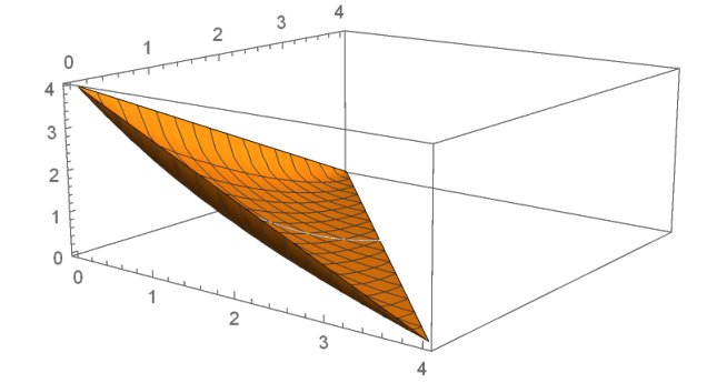
See Figure 2 for an illustration of a representable triple and Figure 1 for an illustration of the set . Note that in any representable triple we have .
Before we can shed light on how we will use representable triples to obtain the desired result, we need to define another concept that is closely related to convexity.
Definition 3.4 (incurved).
We say that a set is incurved if there are no , such that .
Now we are set to give a high-level overview of our approach to prove Lemma 3.2. The “representable triples” from Section 3.2 formalize both the situation at the beginning of the variable fixing performed in Lemma 3.2 and the desired outcome, or more precisely, the part of the situation (resp. outcome) corresponding to subproperty (1) of property : before fixing the variable in question, the values given by add up to at most on each edge, hence the corresponding triple is representable, and Lemma 3.2 assures that the same holds for the values given by after the fixing. The situation before the fixing is worst-case if the respective representable triple lies on the surface bounding the set of all representable triples and if we can find a new representable triple (as the desired outcome, together with a suitable value for the random variable), then we can also find one that lies on this surface. Hence, we can reduce our considerations to this surface. It turns out that the question whether there exists a suitable value for the random variable to be fixed in Lemma 3.2 depends on the shape of this surface: if there is no such suitable value, then the function describing the surface is not convex. However, Lemma 3.5 and Lemma 3.6 show that this function is convex, thereby ensuring that a suitable value exists, which essentially proves Lemma 3.2. For technical reasons, we use the concept of incurvedness (instead of the closely related convexity) for the proof of the relation between the existence of a suitable value for the random variable and the shape of the surface (Lemma 3.9), and show that the convexity of the surface-describing function implies the incurvedness of the set that is bounded by the function (Lemma 3.7). We encourage the reader to consult the plot given in Figure 1 to convince her- or himself that is incurved.
Lemma 3.5.
(Proof Deferred to the Appendix) For we obtain
Lemma 3.6.
(Proof deferred to the Appendix) The function is convex on .
The characterization of given in Lemma 3.5 together with the convexity of from Lemma 3.6 imply that is incurved. The formal proof of this statement is given by Lemma 3.7. Note that Lemma 3.5 and Lemma 3.6 are not crucial to our general approach if one can find a different proof to show that is incurved.
Lemma 3.7.
is incurved.
Proof.
Suppose for a contradiction that there are , with . Let , and set . We consider three cases, depending on the values of and .
- 1.
- 2.
and . In this case, we see that, for any , we have , which implies , by Lemma 3.5, and, again, we obtain a contradiction.
- 3.
and or vice versa. W.l.o.g., we can assume that and . Let be the uniquely defined value such that, for the triple , we have . Observe that if , we can write as , for some , by setting (or if ). But then we obtain a contradiction by applying the argumentation in Case 1 for the triples and . Hence, we know that . Similarly to before, we can write as , for some . In particular, we have which together with and implies that . By Lemma 3.5, , yielding a contradiction. ∎
3.3 Proof of the Variable Fixing Lemma (Lemma 3.2)
Consider the random variable we are about to fix in Lemma 3.2, and assume that it affects the three events located at the nodes which then are connected in the dependency graph by the edges , , and . Recall that our input graph together with the function satisfies . Let the discrete distribution of be given by the set of possible values for and corresponding positive probabilities with which those values occur. For each possible value of we are interested in the increases (or decreases) of the probabilities of our bad events due to fixing . For each value and each , define
If , set .
Now if we can find a value for and values , with , , , such that
then we can prove Lemma 3.2 by identifying and on . In order to find such a value , we will need the definition of an evil value.
Definition 3.8 (evil value).
Let denote the set of all representable triples, and fix some . We call a value of a rank random variable -evil if there exists no such that
In particular, if is -evil, then the triple is not contained in . We prove the following.
Lemma 3.9.
If there exist a rank random variable and a triple such that all possible values for are -evil, then is not incurved.
Proof.
Let and be as described above. Let be the set of possible values for , occurring with positive probabilities . Let denote the bad events affected by , and let denote the associated nodes in the dependency graph, respectively. For , we denote by the probability of bad event to occur conditioned on the values the already fixed random variables have been assigned. By the definition of , we have, for any ,
For , consider the triples defined by . Since is -evil for each , we see that no is contained in . Moreover, by our above observations, we have
Hence, . Consider the sequence of triples defined by and
for all . Let be the smallest index such that . A straighforward induction shows that
Hence, we know that such a exists since as shown above. Moreover, since , we see that . Thus, due to the choice of , by setting , , and
we obtain the desired since . Note that all are elements of as they are weighted averages of elements in , by the characterization of the given above. ∎
Proof of Lemma 3.2.
Recall our setting and observation immediately before Definition 3.8. By combining Lemma 3.7 and Lemma 3.9, we see that for the random variable and the representable triple , there exist a value for and a representable triple such that
Since is representable, there exist values with , , and , , . Hence,
which implies that, for the function completed by identifying and on , the pair satisfies property . Lemma 3.2 follows. ∎
3.4 Proof of the Main Corollary
See 1.4
Proof.
We begin by finding a -hop vertex-coloring of the dependency graph with colors. This can be done in time [FHK16]. Then, we iterate through the color classes and every node of a color class fixes, one by one but in a single communication round, all of its variables that are not fixed yet. We make two observations. First, since we are iterating through a -hop-coloring, no two nodes ever fix variables that share an event. Put otherwise, variables incident on events within at least hops from each other cannot share an event. Second, we are effectively fixing the random variables according to some order on the variables. Since Theorem 1.3 works for any order and due to the local nature of the fixing and bookkeeping in the proof of Theorem 1.3, our process correctly solves the LLL instance. Putting the above together, we obtain an time algorithm for the LLL problem. ∎
Acknowledgements
We thank Mohsen Ghaffari for bringing the considered problem to our attention, together with providing the solution for rank .
References
- [Alo91] Noga Alon. A Parallel Algorithmic Version of the Local Lemma. Random Structures & Algorithms, 2(4):367–378, 1991.
- [Bec91] József Beck. An Algorithmic Approach to the Lovász Local Lemma. Random Structures & Algorithms, 2(4):343–365, 1991.
- [BFH+16] Sebastian Brandt, Orr Fischer, Juho Hirvonen, Barbara Keller, Tuomo Lempiäinen, Joel Rybicki, Jukka Suomela, and Jara Uitto. A Lower Bound for the Distributed Lovász Local Lemma. In the Proceedings of the ACM-SIAM Symposium on Discrete Algorithms (SODA), 2016.
- [BGK+19] Philipp Bamberger, Mohsen Ghaffari, Fabian Kuhn, Yannic Maus, and Jara Uitto. On the complexity of distributed splitting problems. In the Proceedings of the ACM Symposium on Principles of Distributed Computing (PODC). ACM, 2019.
- [BV04] Stephen Boyd and Lieven Vandenberghe. Convex Optimization. Cambridge University Press, 2004.
- [CKP16] Yi-Jun Chang, Tsvi Kopelowitz, and Seth Pettie. An Exponential Separation between Randomized and Deterministic Complexity in the LOCAL Model. In the Proceedings of the Symposium on Foundations of Computer Science (FOCS), pages 615–624, 2016.
- [CP17] Yi-Jun Chang and Seth Pettie. A Time Hierarchy Theorem for the LOCAL Model. In the Proceedings of the Symposium on Foundations of Computer Science (FOCS), pages 156–167, 2017.
- [CPS17] Kai-Min Chung, Seth Pettie, and Hsin-Hao Su. Distributed Algorithms for the Lovász Local Lemma and Graph Coloring. Distributed Computing, 30(4):261–280, 2017.
- [CS00] Artur Czumaj and Christian Scheideler. Coloring Non-uniform Hypergraphs: A New Algorithmic Approach to the General Lovász Local Lemma. In the Proceedings of the ACM-SIAM Symposium on Discrete Algorithms (SODA), pages 30–39, 2000.
- [EL74] Paul Erdös and László Lovász. Problems and Results on 3-chromatic Hypergraphs and some Related Questions. Colloquia Mathematica Societatis János Bolyai, pages 609–627, 1974.
- [FG17] Manuela Fischer and Mohsen Ghaffari. Sublogarithmic Distributed Algorithms for Lovász Local Lemma, and the Complexity Hierarchy. In the Proceedings of the 31st International Symposium on Distributed Computing (DISC), pages 18:1–18:16, 2017.
- [FHK16] Pierre Fraigniaud, Marc Heinrich, and Adrian Kosowski. Local Conflict Coloring. In the Proceedings of the Symposium on Foundations of Computer Science (FOCS), pages 625–634, 2016.
- [Gha16] Mohsen Ghaffari. An Improved Distributed Algorithm for Maximal Independent Set. In the Proceedings of the ACM-SIAM Symposium on Discrete Algorithms (SODA), pages 270–277, 2016.
- [GHK+17] Mohsen Ghaffari, Juho Hirvonen, Fabian Kuhn, Yannic Maus, Jukka Suomela, and Jara Uitto. Improved distributed degree splitting and edge coloring. pages 19:1–19:15, 2017.
- [GHK18] Mohsen Ghaffari, David G. Harris, and Fabian Kuhn. On Derandomizing Local Distributed Algorithms. In the Proceedings of the Symposium on Foundations of Computer Science (FOCS), pages 662–673, 2018.
- [GKM17] Mohsen Ghaffari, Fabian Kuhn, and Yannic Maus. On the complexity of local distributed graph problems. In the Proceedings of the ACM-SIAM Symposium on Discrete Algorithms (SODA), pages 784–797. ACM, 2017.
- [GS17] Mohsen Ghaffari and Hsin-Hao Su. Distributed degree splitting, edge coloring, and orientations. In Proc. 28th ACM-SIAM Symp. on Discrete Algorithms (SODA), 2017.
- [Har18] David G. Harris. Distributed approximation algorithms for maximum matching in graphs and hypergraphs. CoRR, abs/1807.07645, 2018.
- [MR98] Michael Molloy and Bruce Reed. Further Algorithmic Aspects of the Local Lemma. In the Proceedings of the ACM-SIAM Symposium on Discrete Algorithms (SODA), pages 524–529, 1998.
- [MT10] Robin A. Moser and Gábor Tardos. A Constructive Proof of the General Lovász Local Lemma. J. ACM, pages 11:1–11:15, 2010.
- [PR01] Alessandro Panconesi and Romeo Rizzi. Some Simple Distributed Algorithms for Sparse Networks. Distributed Computing, 14(2):97–100, 2001.
- [PT09] János Pach and Gábor Tardos. Conflict-free Colourings of Graphs and Hypergraphs. Combinatorics Probability and Computing, 18(5), 2009.
- [Sri08] Aravind Srinivasan. Improved Algorithmic Versions of the Lovász Local Lemma. In the Proceedings of the ACM-SIAM Symposium on Discrete Algorithms (SODA), pages 611–620, 2008.
- [VG19] Václav Rozhoň and Mohsen Ghaffari. Polylogarithmic-time deterministic network decomposition and distributed derandomization. CoRR, abs/1907.10937, 2019.
Appendix A Deferred Proofs
Proof of Lemma 3.5.
Let We first show that any representable is in . If is representable there are with and . Thus we obtain . We now show that the maximal for which is representable for given with equals . Note that this implies that any is also representable. We consider several cases for and where the only non trivial case is .
- •
Case : We can choose and , i.e, is representable and we also have .
- •
Case : We can choose and . Then we obtain and we also have .
- •
Case : The proof of this case is analogous to the case .
- •
Case . First note that implies because . For fixed we vary the value of to see which values of can be represented. We denote this varying value of by . As we obtain and due to we obtain . Thus we obtain that and . To find the maximal value of we compute the derivative as
Thus we have if and only if .
Case : The equality is satisfied for , that is, .
Case : Let . Then we get if and only if which is satisfied for
The value is outside of the range as for it is negative and for it is larger than . Plugging into yields
Factoring out of the four terms yields and multiplying nominator and denominator with yields As and we have the maximum possible value for for a given with and is . This concludes the case .
Summarizing all cases we have shown that any representable is contained in the set . For the converse direction let , that is, , and . The previous proof has shown that is representable by letting and . As we can also represent by decreasing (or ) without violating the constraints. ∎
Proof of Lemma 3.6.
Set and . Since is continuous on , it is sufficient to show convexity of on the open domain , which in turn can be showed by proving that at every point , the Hessian of is positive semi-definite (cf., e.g., [BV04, Section 3.1.4]). We will prove the slightly stronger statement that is positive definite, which, by Sylvester’s criterion, is equivalent to the statement that all leading principal minors of are positive. In other words, we will prove our lemma by showing that and for all . To this end, we first calculate the four involved terms for . We have
which implies
Since our function is symmetric in and , we also have
Hence, we obtain
for all . Here, the last inequality follows from the fact that, for all , we have since , , and . As argued above, it follows that is convex on . ∎