跳到论文正文
W Papers独立论文阅读器 arXiv:1908.06234 论文正文 计算阅读时间 · 0%
引用这篇论文根据当前论文元数据生成,正式投稿前建议核对。


License: arXiv.org perpetual non-exclusive license
arXiv:1908.06234v2 [astro-ph.CO] 01 Jul 2020

Perturbation theory approach to predict the covariance matrices of the galaxy power spectrum and bispectrum in redshift spacePerturbation theory approach to predict the covariance matrices of the galaxy power spectrum and bispectrum in redshift space–C

Naonori S. Sugiyama Thanks: E-mail: nao.s.sugiyama@gmail.com Affiliation:  National Astronomical Observatory of Japan, Mitaka, Tokyo 181-8588, Japan    Shun Saito Affiliation:  Department of Physics, Missouri University of Science and Technology, 1315 N. Pine St., Rolla MO 65409, USA Affiliation:  Max-Planck-Institut für Astrophysik, Karl-Schwarzschild-Starße 1, D-85740 Garching bei München, Germany Affiliation:  Kavli Institute for the Physics and Mathematics of the Universe (WPI),Todai Institutes for Advanced Study, The University of Tokyo, Chiba 277-8582, Japan    Florian Beutler Affiliation:  Institute of Cosmology & Gravitation, University of Portsmouth, Portsmouth, PO1 3FX, UK Affiliation:  Lawrence Berkeley National Laboratory, 1 Cyclotron Road, Berkeley, CA 94720, USA       Hee-Jong Seo Affiliation:  Department of Physics and Astronomy, Ohio University, Clippinger Labs, Athens, OH 45701
Abstract

In this paper, we predict the covariance matrices of both the power spectrum and the bispectrum, including full non-Gaussian contributions, redshift space distortions, linear bias effects and shot-noise corrections, using perturbation theory (PT). To quantify the redshift-space distortion effect, we focus mainly on the monopole and quadrupole components of both the power and bispectra. We, for the first time, compute the 5- and 6-point spectra to predict the cross-covariance between the power and bispectra, and the auto-covariance of the bispectrum in redshift space. We test the validity of our calculations by comparing them with the covariance matrices measured from the MultiDark-Patchy mock catalogues that are designed to reproduce the galaxy clustering measured from the Baryon Oscillation Spectroscopic Survey Data Release 12. We argue that the simple, leading-order perturbation theory works because the shot-noise corrections for the Patchy mocks are more dominant than other higher-order terms we ignore. In the meantime, we confirm some discrepancies in the comparison, especially of the cross-covariance. We discuss potential sources of such discrepancies. We also show that our PT model reproduces well the cumulative signal-to-noise of the power spectrum and the bispectrum as a function of maximum wavenumber, implying that our PT model captures successfully essential contributions to the covariance matrices.

Keywords: 
cosmology: large-scale structure of Universe – cosmology: dark matter – cosmology: observations – cosmology: theory

1 INTRODUCTION

It is essential to measure higher order statistics beyond the two-point statistics to extract the full cosmological information, as the galaxy density field at low redshift is strongly non-Gaussian due to non-linear structure formation and galaxy bias. Given the greatly successful analyses of the two-point statistics in galaxy redshift surveys (e.g., see Alam et al. 2017 and references therein), the focus has been recently shifting to higher order statistics, i.e., the three-point correlation function or its Fourier space counterpart, the bispectrum. Over the past few years, some applications to use the the three-point statistics to constrain cosmological parameters have been made (as recent works, e.g.,  Slepian et al. 2017; Gil-Marln et al. 2017; Pearson & Samushia 2018). The joint analysis of the two- and three-point statistics will thus continue to be a standard method for analyzing galaxy data in future galaxy redshift surveys: e.g., the Subaru Prime Focus Spectrograph (PFS;  Takada et al. 2014), the Dark Energy Spectroscopic Instrument (DESI; Levi et al. 2013), the Euclid mission (Laureijs et al. 2011) and the Wide Field Infrared Survey Telescope (WFIRST; Akeson et al. 2019). To correctly interpret the upcoming high quality datasets, accurate modeling not only of the nonlinear power spectrum and the bispecutrm but also of their statistical uncertainties, i.e., covariance matrices, is of crucial importance.

A common approach to estimate the covariance matrix is to utilize hundreds or thousands of synthetic realizations generated by fast approximate schemes to create galaxy catalogues, e.g., the Quick-Particle-Mesh (QPM; White et al. 2014) mocks, the MultiDark-Patchy (MD-Patchy; Klypin et al. 2016; Kitaura et al. 2016) mocks, the Effective Zel’dovich approximation (EZ; Chuang et al. 2015) mocks, and log-normal mocks (Agrawal et al. 2017). However, there are two issues for the estimates of the covariance matrix from the mock catalogues. First, such brute-force production suffers from the noise due to the finite number of realizations, and uncertainties on the invert covariance matrix estimate propagate directly to increased uncertainties on cosmological parameters (Hartlap et al. 2006; Taylor et al. 2013; Dodelson & Schneider 2013; Percival et al. 2014; Taylor & Joachimi 2014). The situation becomes worse in the joint analysis of the power spectrum and the bispectrum, because it requires about 10 or 20 times larger number of data bins than the power spectrum only analysis (Sugiyama et al. 2019), substantially increasing the required number of independent realizations. To reduce the computational cost of mock generation, various other approaches have been proposed for the power spectrum analysis (Hamilton et al. 2006; Pope & Szapudi 2008; Schneider et al. 2011; Paz & Sanchez 2015; Pearson & Samushia 2016; Padmanabhan et al. 2016; O’Connell et al. 2016; Howlett & Percival 2017; Escoffier et al. 2016; Takahashi et al. 2018). Second, aforementioned fast mock generation schemes are typically designed to only reproduce the observed 2-point function for a target galaxy sample, and hence it is not entirely clear if they can reproduce the 3-point functions at the same time. These difficulties associated with the mock-based approach motivate an analytical approach as a complementary way to estimate the covariance matrix. An analytical approach does not suffer from the issues discussed above, albeit its accuracy should be confirmed by ideal mock galaxy simulations. Therefore it is highly desirable to develop an analytic model to predict the covariance matrices.

From a theoretical point of view, the covariance matrix can be expressed with unconnected and connected parts, the so-called Gaussian and non-Gaussian terms, respectively. To evaluate the non-Gaussian terms, one needs to take into account statistics beyond the power spectrum and bispectrum: namely, the trispectrum, the 5-point and the 6-point spectrum in Fourier space, as we will explicitly show later. In the case of the two-point statistics, the analytical expression in the Gaussian limit was first shown in e.g., Feldman et al. 1994; subsequently, perturbation theory was often adopted to assess the impact of the non-Gaussian term (the trispectrum) on the matter (halo) power spectrum covariances  (Meiksin & White 1999; Eisenstein & Zaldarriaga 2001; Smith 2009; Carron et al. 2015; Bertolini et al. 2016; Mohammed et al. 2017; Barreira & Schmidt 2017a; Barreira & Schmidt 2017b; Howlett & Percival 2017) and the weak lensing power spectrum covariances (Scoccimarro et al. 1999b; Reischke et al. 2017; Barreira et al. 2018). In addition, the halo model approach (for a review, see Cooray & Sheth 2002) has been used to estimate the covariance matrix for the matter (halo) (Neyrinck et al. 2006; Neyrinck & Szapudi 2007; Wu & Huterer 2013; Mohammed & Seljak 2014; Ginzburg et al. 2017; Takada & Hu 2013) and weak lensing power spectra (Cooray & Hu 2001; Takada & Bridle 2007; Takada & Jain 2009; Takahashi et al. 2018). Since these analytical models are unable to capture full non-linear gravitational effects on small scales, one also often uses NN-body simulations for a better understanding of the non-Gaussian effect and for testing the validity of these models (Rimes & Hamilton 2006; Neyrinck & Szapudi 2008; Takahashi et al. 2009; Takahashi et al. 2011; Sato et al. 2009; Ngan et al. 2012; de Putter et al. 2012; Blot et al. 2015; Blot et al. 2016; Blot et al. 2018).

The bispectrum covariance is far less well understood compared to the power spectrum case. Kayo et al. 2013; Kayo & Takada 2013 addressed the amount of information included in the lensing power and bispectra using the halo model approach as well as ray-tracing simulations, but took into account the contribution only from the 1-halo term to the 6-point function. Chan & Blot 2017; Chan et al. 2018 measured the 3-dimensional (3D) matter and halo bispectrum covariances from NN-body simulations in real space and computed a part of non-Gaussian terms of the bispectrum covariance using perturbation theory, ignoring the 6-point function. Gualdi et al. 2018; Gualdi et al. 2019 have computed a part of non-Gaussian terms of the bispectrum covariance, as well as the cross-covariance between the power and bispectra, using perturbation theory in redshift-space. Colavincenzo et al. 2018 has compared the bispectrum “monopole” measurements and their covariances in both real and redshift spaces from a set of different methods for the efficient generation of approximate dark matter catalogues.

Despite all the work discussed above, there is still a limited understanding of the analytical covariance in redshift space. The observed 3D galaxy clustering is distorted along the line of sight (LOS) because of the peculiar velocities of galaxies (Kaiser 1987), known as redshift space distortion (RSD; see Hamilton 1997 for a review). An additional anisotropic signal arises due to the conversion from the observed redshifts into radial distances with incorrect cosmological parameters, which is known as the Alcock-Paczyński (AP) effect (Alcock & Paczyński 1979). To single out only the anisotropic signal, we commonly decompose the power spectrum (e.g., Hamilton 1997) and the bispectrum (Scoccimarro et al. 1999a; Sugiyama et al. 2019; Slepian & Eisenstein 2018) into multipole components regarding the angle with respect to the LOS direction. In particular, we have recently proposed a new decomposition formalism for the redshift-space bispectrum, based on the tri-polar spherical harmonic (TriPoSH) formalism (Sugiyama et al. 2019), and showed the advantages of our novel formalism including the survey window function; throughout this paper, we adopt our decomposed multipole components of the bispectrum to explore their covariances. We note that, while the Gaussian term of the covariance of the power spectrum multipoles has been well studied in Grieb et al. 2016; Li et al. 2019, the theoretical modeling of non-Gaussian contributions to the covariances of the power spectrum and especially of the bispectrum has not been investigated in detail.

The aim of this paper is therefore to develop a simple model for the galaxy power spectrum and bispectrum covariances, including the full non-Gaussian parts up to the 6-point spectrum, the RSD effect, the linear bias and the shot-noise corrections, which will enable us to compare our calculations with the covariances estimated from realistic mock simulations. For this purpose, we adopt the standard perturbation theory (PT; for a review, see Bernardeau et al. 2002) and compute up to the leading order, i.e., the tree level. This requires the fifth order of perturbation solutions of density fluctuations, because the trispectrum (4-point), the 5-point and the 6-point spectra calculations require the third, fourth and fifth order of the perturbation theory, respectively. We test the validity of our PT calculations by comparing them with the Multidark Patchy mock catalogues (Klypin et al. 2016; Kitaura et al. 2016) that are designed to reproduce the galaxy data set measured from the Baryon Oscillation Spectroscopic Survey Data Release 12 (BOSS DR12; Alam et al. 2015). We remark that, in our previous work (Sugiyama et al. 2019), we showed that the Patchy mock catalogs can reproduce the bispectrum multipoles of the observed BOSS data. We will show good agreement of the PT calculations with the mock results of the covariance matrices for the power spectrum and bispectrum up to the scales of ∼0.2​h​Mpc−1\sim 0.2\,h\,{\rm Mpc^{-1}}.

To predict the covariances of the power and bispectrum measured from discrete samples, i.e., galaxy samples, the Poisson shot-noise remains an issue, which is highly relevant to the off-diagonal component in the covariances. As pointed out in Smith 2009 using NN-body simulations, there is a difference between the covariance matrices estimated from the halo power spectrum measurements without and with the shot-noise subtraction: namely, the off-diagonal correlation that is present in the shot-noise uncorrected covariance are suppressed in the shot-noise corrected covariance. This result implies that, since the total number of halos (galaxies) varies between realizations, there are additional sources of covariance that originate from the cross-correlation between the halo (galaxy) power spectrum and the number density as well as the variance of the number density, but such correlations relevant to the shot-noise term are mostly removed by the shot-noise subtraction. Chan & Blot 2017 discussed a similar behavior for the halo bispectrum covariance. In the case of the two-point correlation function, O’Connell et al. 2016 has shown the covariance expression accounting for removing the self-counting of galaxies corresponding to the shot-noise term in Fourier space. In this paper, we work in Fourier space and will show the analytic expressions of the shot-noise corrected covariances in both the power spectrum and bispectrum, and address its impact on the non-Gaussian contribution of the covariances.

The plan of this paper is as follows. Section 2 presents the analytical expressions of the covariance matrices of the power spectrum and the bispectrum. Section 3 reviews the decomposition formalism of the redshift-space power spectrum and bispectrum. We test the validation of our analytical calculations by comparing them with the Patchy mock results in Section 4. To estimate the impact of the non-Gaussian errors, we compute the cumulative signal-to-noise ratios in 5. The conclusions and discussion are summarized in Section 6. Throughout this paper, we adopt a flat Λ\LambdaCDM cosmology that is the same as used in the Patchy mocks: (ΩΛ,Ωm,Ωb,σ8,h)=(0.693,0.307,0.0480,0.829,0.678)(\Omega_{\Lambda},\Omega_{\rm m},\Omega_{\rm b},\sigma_{8},h)=(0.693,0.307,0.0480,0.829,0.678).

2 Covariance model

The goal of this paper is to provide an analytic model of the covariance matrices for both the power spectrum and the bispectrum on the basis of PT, and to compare them with the covariance matrices measured from the Patchy mock catalogs to test the validity of the perturbation theory calculations. In this section, we present exact formulae to describe the covariance matrices. More concretely, we show the representations of the power, bi, tri, 5-point and 6-point spectra in a discretized picture in Section 2.1, and derive the analytic expressions of the auto-covariances of both the power spectrum and the bispectrum, as well as the cross-covariance between the power spectrum and the bispectrum, with the shot-noise term subtracted from the power- and bi-spectrum measurements, in Sections 2.2, 2.4 and 2.5. Throughout this paper, we ignore non-linear corrections on the covariance matrix such as higher-order loop corrections, including the Finger-of-God effect, non-linear bias effects, and the super-sample covariance (SSC) effect. We summarize the limitation of our analytical calculations in Section 2.6.

For notational simplicity, we omit to denote the redshift- and LOS-dependence on all statistics that we compute: e.g., the redshift-space power spectrum P⁡(𝒌,n^,z)P(\mn@boldsymbol{k},\hat{n},z), with 𝒌\mn@boldsymbol{k}, n^\hat{n} and zz being respectively wavevector, the unit vector orienting to the LOS direction and redshift, is represented just as P⁡(𝒌)P(\mn@boldsymbol{k}). In Appendix A, we present our PT approach to evaluate the expressions shown here.

2.1 NN-point Statistics in a discretized picture

Following Peebles 1980, the Fourier transform of the galaxy number density, n⁡(𝒙)n(\mn@boldsymbol{x}), is discretized as follows:

n(𝒌)=∫d3xe−i𝒌⋅𝒙n(𝒙)→∑inie−i𝒌⋅𝒙i,\displaystyle n(\mn@boldsymbol{k})=\int d^{3}x\,e^{-i\mn@boldsymbol{k}\cdot\mn@boldsymbol{x}}\,n(\mn@boldsymbol{x})\to\sum_{i}\,n_{i}\,e^{-i\mn@boldsymbol{k}\cdot\mn@boldsymbol{x}_{i}}, (1)

where we divide the space into the infinitesimal grid cells of volume δ​V\delta V. Each cell is allowed to contain at most one galaxy, which can be described by the occupation number ni=n⁡(𝒙i)​δ​Vn_{i}=n(\mn@boldsymbol{x}_{i})\delta V such that ni=1n_{i}=1 if the ii-th cell has a galaxy, otherwise ni=0n_{i}=0, and therefore, it satisfies ni=ni2=⋯=ninn_{i}=n_{i}^{2}=\dots=n_{i}^{n}. The total number of galaxies, NN, is then given by N=∑i⟨ni⟩cN=\sum_{i}\langle n_{i}\rangle_{\rm c}, where ⟨⋯⟩c\langle\cdots\rangle_{\rm c} denotes a cumulant of the ensemble average. The background (unperturbed) number density, which is defined as n¯=N/V\bar{n}=N/V with VV being the survey volume, is measured by the 𝒌=0\mn@boldsymbol{k}=0 mode of the ensemble average of the galaxy number density: namely, ⟨n⁡(𝒌)⟩c=(2​π)3​δD​(𝒌)​n¯\langle n(\mn@boldsymbol{k})\rangle_{\rm c}=(2\pi)^{3}\delta_{\rm D}\left(\mn@boldsymbol{k}\right)\bar{n}, where δD\delta_{\rm D} represents the Dirac delta function. This fact indicates that n⁡(𝒌)n(\mn@boldsymbol{k}) at 𝒌≠𝟎\mn@boldsymbol{k}\neq\mn@boldsymbol{0} is a perturbed quantity.

The power spectrum is then represented in the discretized description as

VN2​⟨n⁡(𝒌)​n​(𝒌′)⟩c\displaystyle\frac{V}{N^{2}}\left\langle n(\mn@boldsymbol{k})n(\mn@boldsymbol{k}^{\prime})\right\rangle_{\rm c} =\displaystyle= (2​π)3​δD​(𝒌+𝒌′)V[VN2∑i≠j⟨ninj⟩ce−i𝒌⋅(𝒙i−𝒙j)+VN2∑i⟨ni2⟩c]\displaystyle\frac{(2\pi)^{3}\delta_{\rm D}\left(\mn@boldsymbol{k}+\mn@boldsymbol{k}^{\prime}\right)}{V}\,\left[\frac{V}{N^{2}}\sum_{i\neq j}\left\langle n_{i}n_{j}\right\rangle_{\rm c}e^{-i\mn@boldsymbol{k}\cdot(\mn@boldsymbol{x}_{i}-\mn@boldsymbol{x}_{j})}+\frac{V}{N^{2}}\sum_{i}\left\langle n_{i}^{2}\right\rangle_{\rm c}\right] (2)
=\displaystyle= (2​π)3​δD​(𝒌+𝒌′)V​[P​(𝒌)+1n¯],\displaystyle\frac{(2\pi)^{3}\delta_{\rm D}\left(\mn@boldsymbol{k}+\mn@boldsymbol{k}^{\prime}\right)}{V}\,\left[P(\mn@boldsymbol{k})+\frac{1}{\bar{n}}\right],

where 𝒌≠𝟎\mn@boldsymbol{k}\neq\mn@boldsymbol{0}, 𝒌′≠𝟎\mn@boldsymbol{k}^{\prime}\neq\mn@boldsymbol{0}, and in the second line of the above expression, we used ∑i⟨ni2⟩c=∑i⟨ni⟩c=N\sum_{i}\langle n_{i}^{2}\rangle_{\rm c}=\sum_{i}\langle n_{i}\rangle_{\rm c}=N. From Eq. (2), the power spectrum estimator is derived as

P^​(𝒌,𝒌′)\displaystyle\widehat{P}(\mn@boldsymbol{k},\mn@boldsymbol{k}^{\prime}) =\displaystyle= VN2∑i,jninje−i𝒌⋅𝒙ie−i𝒌′⋅𝒙j−VN2∑i=jni2e−i(𝒌+𝒌′)⋅𝒙i\displaystyle\frac{V}{N^{2}}\sum_{i,j}n_{i}n_{j}e^{-i\mn@boldsymbol{k}\cdot\mn@boldsymbol{x}_{i}}e^{-i\mn@boldsymbol{k}^{\prime}\cdot\mn@boldsymbol{x}_{j}}-\frac{V}{N^{2}}\sum_{i=j}n_{i}^{2}e^{-i(\mn@boldsymbol{k}+\mn@boldsymbol{k}^{\prime})\cdot\mn@boldsymbol{x}_{i}} (3)
=\displaystyle= VN2∑i≠jninje−i𝒌⋅𝒙ie−i𝒌′⋅𝒙j,\displaystyle\frac{V}{N^{2}}\sum_{i\neq j}n_{i}n_{j}e^{-i\mn@boldsymbol{k}\cdot\mn@boldsymbol{x}_{i}}e^{-i\mn@boldsymbol{k}^{\prime}\cdot\mn@boldsymbol{x}_{j}},

which satisfies

⟨P^​(𝒌,𝒌′)⟩c=(2​π)3​δD​(𝒌+𝒌′)V​P​(𝒌).\displaystyle\langle\widehat{P}(\mn@boldsymbol{k},\mn@boldsymbol{k}^{\prime})\rangle_{\rm c}=\frac{(2\pi)^{3}\delta_{\rm D}\left(\mn@boldsymbol{k}+\mn@boldsymbol{k}^{\prime}\right)}{V}P(\mn@boldsymbol{k}). (4)

We stress that the condition in this estimator, i≠ji\neq j, ensures that the Poisson shot noise, i.e., the second term in the first line of Eq. (3), is subtracted out.

Similarly, the estimators of higher order statistics, the bispectrum, the trispectrum, the 5-point spectrum and the 6-point spectrum, are given by

B^​(𝒌1,𝒌2,𝒌3)\displaystyle\widehat{B}(\mn@boldsymbol{k}_{1},\mn@boldsymbol{k}_{2},\mn@boldsymbol{k}_{3}) =\displaystyle= (V2/N3)∑i≠j≠kninjnke−i𝒌1⋅𝒙ie−i𝒌2⋅𝒙je−i𝒌3⋅𝒙k\displaystyle(V^{2}/N^{3})\sum_{i\neq j\neq k}n_{i}n_{j}n_{k}\,e^{-i\mn@boldsymbol{k}_{1}\cdot\mn@boldsymbol{x}_{i}}e^{-i\mn@boldsymbol{k}_{2}\cdot\mn@boldsymbol{x}_{j}}e^{-i\mn@boldsymbol{k}_{3}\cdot\mn@boldsymbol{x}_{k}}
T^​(𝒌1,𝒌2,𝒌3,𝒌4)\displaystyle\widehat{T}(\mn@boldsymbol{k}_{1},\mn@boldsymbol{k}_{2},\mn@boldsymbol{k}_{3},\mn@boldsymbol{k}_{4}) =\displaystyle= (V3/N4)∑i≠j≠k≠lninjnknle−i𝒌1⋅𝒙ie−i𝒌2⋅𝒙je−i𝒌3⋅𝒙ke−i𝒌4⋅𝒙l\displaystyle(V^{3}/N^{4})\sum_{i\neq j\neq k\neq l}n_{i}n_{j}n_{k}n_{l}\,e^{-i\mn@boldsymbol{k}_{1}\cdot\mn@boldsymbol{x}_{i}}e^{-i\mn@boldsymbol{k}_{2}\cdot\mn@boldsymbol{x}_{j}}e^{-i\mn@boldsymbol{k}_{3}\cdot\mn@boldsymbol{x}_{k}}e^{-i\mn@boldsymbol{k}_{4}\cdot\mn@boldsymbol{x}_{l}}
P^5​(𝒌1,𝒌2,𝒌3,𝒌4,𝒌5)\displaystyle\widehat{P}_{5}(\mn@boldsymbol{k}_{1},\mn@boldsymbol{k}_{2},\mn@boldsymbol{k}_{3},\mn@boldsymbol{k}_{4},\mn@boldsymbol{k}_{5}) =\displaystyle= (V4/N5)∑i≠j≠k≠l≠mninjnknlnme−i𝒌1⋅𝒙ie−i𝒌2⋅𝒙je−i𝒌3⋅𝒙ke−i𝒌4⋅𝒙le−i𝒌5⋅𝒙m\displaystyle(V^{4}/N^{5})\hskip-5.69046pt\sum_{i\neq j\neq k\neq l\neq m}\hskip-5.69046ptn_{i}n_{j}n_{k}n_{l}n_{m}\,e^{-i\mn@boldsymbol{k}_{1}\cdot\mn@boldsymbol{x}_{i}}e^{-i\mn@boldsymbol{k}_{2}\cdot\mn@boldsymbol{x}_{j}}e^{-i\mn@boldsymbol{k}_{3}\cdot\mn@boldsymbol{x}_{k}}e^{-i\mn@boldsymbol{k}_{4}\cdot\mn@boldsymbol{x}_{l}}e^{-i\mn@boldsymbol{k}_{5}\cdot\mn@boldsymbol{x}_{m}}
P^6​(𝒌1,𝒌2,𝒌3,𝒌4,𝒌5,𝒌6)\displaystyle\widehat{P}_{6}(\mn@boldsymbol{k}_{1},\mn@boldsymbol{k}_{2},\mn@boldsymbol{k}_{3},\mn@boldsymbol{k}_{4},\mn@boldsymbol{k}_{5},\mn@boldsymbol{k}_{6}) =\displaystyle= (V5/N6)∑i≠j≠k≠l≠m≠nninjnknlnmnne−i𝒌1⋅𝒙ie−i𝒌2⋅𝒙je−i𝒌3⋅𝒙ke−i𝒌4⋅𝒙le−i𝒌5⋅𝒙me−i𝒌6⋅𝒙n.\displaystyle(V^{5}/N^{6})\hskip-8.5359pt\sum_{i\neq j\neq k\neq l\neq m\neq n}\hskip-8.5359ptn_{i}n_{j}n_{k}n_{l}n_{m}n_{n}\,e^{-i\mn@boldsymbol{k}_{1}\cdot\mn@boldsymbol{x}_{i}}e^{-i\mn@boldsymbol{k}_{2}\cdot\mn@boldsymbol{x}_{j}}e^{-i\mn@boldsymbol{k}_{3}\cdot\mn@boldsymbol{x}_{k}}e^{-i\mn@boldsymbol{k}_{4}\cdot\mn@boldsymbol{x}_{l}}e^{-i\mn@boldsymbol{k}_{5}\cdot\mn@boldsymbol{x}_{m}}e^{-i\mn@boldsymbol{k}_{6}\cdot\mn@boldsymbol{x}_{n}}. (5)

Note that all these estimators are contributed only by density correlations among different positions. Namely, the self-counting of galaxies is all removed: e.g., i≠j≠ki\neq j\neq k includes the condition i≠ki\neq k, and i≠j≠k≠li\neq j\neq k\neq l means i≠ki\neq k, i≠li\neq l and j≠lj\neq l. Similar results hold also for i≠j≠k≠l≠mi\neq j\neq k\neq l\neq m and i≠j≠k≠l≠m≠ni\neq j\neq k\neq l\neq m\neq n. Therefore, these estimators do not include the shot noise effect. They satisfy

⟨B^​(𝒌1,𝒌2,𝒌3)⟩c\displaystyle\langle\widehat{B}(\mn@boldsymbol{k}_{1},\mn@boldsymbol{k}_{2},\mn@boldsymbol{k}_{3})\rangle_{\rm c} =\displaystyle= (2​π)3​δD​(𝒌123)V​B​(𝒌1,𝒌2,𝒌3)\displaystyle\frac{(2\pi)^{3}\delta_{\rm D}\left(\mn@boldsymbol{k}_{123}\right)}{V}B(\mn@boldsymbol{k}_{1},\mn@boldsymbol{k}_{2},\mn@boldsymbol{k}_{3})
⟨T^​(𝒌1,𝒌2,𝒌3,𝒌4)⟩c\displaystyle\langle\widehat{T}(\mn@boldsymbol{k}_{1},\mn@boldsymbol{k}_{2},\mn@boldsymbol{k}_{3},\mn@boldsymbol{k}_{4})\rangle_{\rm c} =\displaystyle= (2​π)3​δD​(𝒌1234)V​T​(𝒌1,𝒌2,𝒌3,𝒌4)\displaystyle\frac{(2\pi)^{3}\delta_{\rm D}\left(\mn@boldsymbol{k}_{1234}\right)}{V}T(\mn@boldsymbol{k}_{1},\mn@boldsymbol{k}_{2},\mn@boldsymbol{k}_{3},\mn@boldsymbol{k}_{4})
⟨P^5​(𝒌1,𝒌2,𝒌3,𝒌4,𝒌5)⟩c\displaystyle\langle\widehat{P}_{5}(\mn@boldsymbol{k}_{1},\mn@boldsymbol{k}_{2},\mn@boldsymbol{k}_{3},\mn@boldsymbol{k}_{4},\mn@boldsymbol{k}_{5})\rangle_{\rm c} =\displaystyle= (2​π)3​δD​(𝒌12345)V​P5​(𝒌1,𝒌2,𝒌3,𝒌4,𝒌5)\displaystyle\frac{(2\pi)^{3}\delta_{\rm D}\left(\mn@boldsymbol{k}_{12345}\right)}{V}P_{5}(\mn@boldsymbol{k}_{1},\mn@boldsymbol{k}_{2},\mn@boldsymbol{k}_{3},\mn@boldsymbol{k}_{4},\mn@boldsymbol{k}_{5})
⟨P^6​(𝒌1,𝒌2,𝒌3,𝒌4,𝒌5,𝒌6)⟩c\displaystyle\langle\widehat{P}_{6}(\mn@boldsymbol{k}_{1},\mn@boldsymbol{k}_{2},\mn@boldsymbol{k}_{3},\mn@boldsymbol{k}_{4},\mn@boldsymbol{k}_{5},\mn@boldsymbol{k}_{6})\rangle_{\rm c} =\displaystyle= (2​π)3​δD​(𝒌123456)V​P6​(𝒌1,𝒌2,𝒌3,𝒌4,𝒌5,𝒌6),\displaystyle\frac{(2\pi)^{3}\delta_{\rm D}\left(\mn@boldsymbol{k}_{123456}\right)}{V}P_{6}(\mn@boldsymbol{k}_{1},\mn@boldsymbol{k}_{2},\mn@boldsymbol{k}_{3},\mn@boldsymbol{k}_{4},\mn@boldsymbol{k}_{5},\mn@boldsymbol{k}_{6}), (6)

where 𝒌1≠𝟎\mn@boldsymbol{k}_{1}\neq\mn@boldsymbol{0}, 𝒌2≠𝟎\mn@boldsymbol{k}_{2}\neq\mn@boldsymbol{0}, 𝒌3≠𝟎\mn@boldsymbol{k}_{3}\neq\mn@boldsymbol{0}, 𝒌4≠𝟎\mn@boldsymbol{k}_{4}\neq\mn@boldsymbol{0}, 𝒌5≠𝟎\mn@boldsymbol{k}_{5}\neq\mn@boldsymbol{0}, 𝒌6≠𝟎\mn@boldsymbol{k}_{6}\neq\mn@boldsymbol{0}, and 𝒌1​…​n=𝒌1+⋯+𝒌n\mn@boldsymbol{k}_{1\dots n}=\mn@boldsymbol{k}_{1}+\dots+\mn@boldsymbol{k}_{n}. We stress again that these higher order statistics defined above are the quantities with the self-counting of galaxies, i.e. the shot-noise, removed. To correctly estimate the signal of the measured statistics, the shot-noise subtraction is crucial, because the amplitude of the bispectrum monopole becomes comparable to or even smaller than that of the corresponding shot-noise term at scales of k≳0.1​h​Mpc−1k\gtrsim 0.1\,h\,{\rm Mpc^{-1}} for the BOSS sample (Sugiyama et al. 2019). We expect similar results for higher order statistics. As we will show in Section 2.3, the shot-noise subtraction is also crucial for suppressing the off-diagonal component of the covariance.

2.2 Power spectrum covariance

The power spectrum covariance can be decomposed into two contributions:

Cov⁡[P^​(𝒌),P^​(𝒌′)]=Cov​[P^​(𝒌),P^​(𝒌′)]P​P+Cov​[P^​(𝒌),P^​(𝒌′)]T,\displaystyle{\rm Cov}\big[\widehat{P}(\mn@boldsymbol{k}),\widehat{P}(\mn@boldsymbol{k}^{\prime})\big]={\rm Cov}\big[\widehat{P}(\mn@boldsymbol{k}),\widehat{P}(\mn@boldsymbol{k}^{\prime})\big]_{PP}+{\rm Cov}\big[\widehat{P}(\mn@boldsymbol{k}),\widehat{P}(\mn@boldsymbol{k}^{\prime})\big]_{T}, (7)

where the first and second terms on the right hand side (RHS) denote the Gaussian and non-Gaussian parts, respectively. The subscripts “P​PPP” and “TT” indicate that the Gaussian part consists of the product of two power spectra (PP), and that the non-Gaussian part arises from the trispectrum (TT), respectively.

To correctly derive the auto-covariance of the galaxy power spectrum with shot-noise corrections, we use the discretized representation of the power spectrum estimator (3); then, the power spectrum covariance can be represented as

Cov⁡[P^​(𝒌),P^​(𝒌′)]\displaystyle{\rm Cov}\big[\widehat{P}(\mn@boldsymbol{k}),\widehat{P}(\mn@boldsymbol{k}^{\prime})\big] =\displaystyle= (VN2)2∑i≠j∑k≠le−i𝒌⋅(𝒙i−𝒙j)e−i𝒌′⋅(𝒙k−𝒙l)[⟨nink⟩c⟨njnl⟩c+⟨ninl⟩c⟨njnk⟩c+⟨ninjnknl⟩c].\displaystyle\left(\frac{V}{N^{2}}\right)^{2}\sum_{i\neq j}\sum_{k\neq l}e^{-i\mn@boldsymbol{k}\cdot(\mn@boldsymbol{x}_{i}-\mn@boldsymbol{x}_{j})}e^{-i\mn@boldsymbol{k}^{\prime}\cdot(\mn@boldsymbol{x}_{k}-\mn@boldsymbol{x}_{l})}\left[\langle n_{i}n_{k}\rangle_{\rm c}\langle n_{j}n_{l}\rangle_{\rm c}+\langle n_{i}n_{l}\rangle_{\rm c}\langle n_{j}n_{k}\rangle_{\rm c}+\langle n_{i}n_{j}n_{k}n_{l}\rangle_{\rm c}\right]. (8)

The first two terms on the RHS correspond to the Gaussian part, given by

Cov​[P^​(𝒌),P^​(𝒌′)]P​P\displaystyle{\rm Cov}\big[\widehat{P}(\mn@boldsymbol{k}),\widehat{P}(\mn@boldsymbol{k}^{\prime})\big]_{PP} =\displaystyle= (VN2)2[∑i,k⟨nink⟩ce−i𝒌⋅𝒙ie−i𝒌′⋅𝒙k][∑j,l⟨njnl⟩cei​𝒌⋅𝒙jei​𝒌′⋅𝒙l]+(1 perm.).\displaystyle\left(\frac{V}{N^{2}}\right)^{2}\bigg[\sum_{i,k}\langle n_{i}n_{k}\rangle_{\rm c}e^{-i\mn@boldsymbol{k}\cdot\mn@boldsymbol{x}_{i}}e^{-i\mn@boldsymbol{k}^{\prime}\cdot\mn@boldsymbol{x}_{k}}\bigg]\bigg[\sum_{j,l}\langle n_{j}n_{l}\rangle_{\rm c}e^{i\mn@boldsymbol{k}\cdot\mn@boldsymbol{x}_{j}}e^{i\mn@boldsymbol{k}^{\prime}\cdot\mn@boldsymbol{x}_{l}}\bigg]+\mbox{(1 perm.)}. (9)

Using Eq. (2), the Gaussian term becomes the well-known form

Cov​[P^​(𝒌),P^​(𝒌′)]P​P=(2​π)3​δD​(𝒌+𝒌′)+(2​π)3​δD​(𝒌−𝒌′)V​[P(N)​(𝒌)]2,\displaystyle{\rm Cov}\big[\widehat{P}(\mn@boldsymbol{k}),\widehat{P}(\mn@boldsymbol{k}^{\prime})\big]_{PP}=\frac{(2\pi)^{3}\delta_{\rm D}(\mn@boldsymbol{k}+\mn@boldsymbol{k}^{\prime})+(2\pi)^{3}\delta_{\rm D}(\mn@boldsymbol{k}-\mn@boldsymbol{k}^{\prime})}{V}\left[P^{(\rm N)}(\mn@boldsymbol{k})\right]^{2}, (10)

where we define the power spectrum with the shot-noise term as

P(N)​(𝒌)≡P⁡(𝒌)+1n¯.\displaystyle P^{(\rm N)}(\mn@boldsymbol{k})\equiv P(\mn@boldsymbol{k})+\frac{1}{\bar{n}}. (11)

As well known, here the shot noise effect on the power spectrum covariance remains even after shot noise correction due to the contribution from e.g., i=ki=k or j=lj=l terms. The third term on the RHS of Eq. (8), i.e., the non-Gaussian part, is given by

Cov​[P^​(𝒌),P^​(𝒌′)]T\displaystyle{\rm Cov}\big[\widehat{P}(\mn@boldsymbol{k}),\widehat{P}(\mn@boldsymbol{k}^{\prime})\big]_{T} =\displaystyle= (V/N2)2∑(i≠j),(k≠l)⟨ninjnknl⟩ce−i𝒌⋅𝒙iei​𝒌⋅𝒙je−i𝒌′⋅𝒙kei​𝒌′⋅𝒙l\displaystyle(V/N^{2})^{2}\sum_{(i\neq j),(k\neq l)}\langle n_{i}n_{j}n_{k}n_{l}\ \rangle_{\rm c}\,e^{-i\mn@boldsymbol{k}\cdot\mn@boldsymbol{x}_{i}}e^{i\mn@boldsymbol{k}\cdot\mn@boldsymbol{x}_{j}}e^{-i\mn@boldsymbol{k}^{\prime}\cdot\mn@boldsymbol{x}_{k}}e^{i\mn@boldsymbol{k}^{\prime}\cdot\mn@boldsymbol{x}_{l}} (12)
=\displaystyle= (V/N2)2∑i≠j≠k≠l⟨ninjnknl⟩ce−i𝒌⋅𝒙iei​𝒌⋅𝒙je−i𝒌′⋅𝒙kei​𝒌′⋅𝒙l\displaystyle(V/N^{2})^{2}\sum_{i\neq j\neq k\neq l}\langle n_{i}n_{j}n_{k}n_{l}\ \rangle_{\rm c}\,e^{-i\mn@boldsymbol{k}\cdot\mn@boldsymbol{x}_{i}}e^{i\mn@boldsymbol{k}\cdot\mn@boldsymbol{x}_{j}}e^{-i\mn@boldsymbol{k}^{\prime}\cdot\mn@boldsymbol{x}_{k}}e^{i\mn@boldsymbol{k}^{\prime}\cdot\mn@boldsymbol{x}_{l}}
+\displaystyle+ (V/N2)2[∑(i≠j≠l),(i=k)⟨ni2njnl⟩ce−i(𝒌+𝒌′)⋅𝒙iei​𝒌⋅𝒙jei​𝒌′⋅𝒙l+(3 perms.)]\displaystyle(V/N^{2})^{2}\Big[\sum_{(i\neq j\neq l),(i=k)}\langle n_{i}^{2}n_{j}n_{l}\ \rangle_{\rm c}\,e^{-i(\mn@boldsymbol{k}+\mn@boldsymbol{k}^{\prime})\cdot\mn@boldsymbol{x}_{i}}e^{i\mn@boldsymbol{k}\cdot\mn@boldsymbol{x}_{j}}e^{i\mn@boldsymbol{k}^{\prime}\cdot\mn@boldsymbol{x}_{l}}+\mbox{(3 perms.)}\Big]
+\displaystyle+ (V/N2)2[∑(i≠j),(i=k),(j=l)⟨ni2nj2⟩ce−i(𝒌+𝒌′)⋅𝒙iei⁡(𝒌+𝒌′)⋅𝒙j+(1 perm.)].\displaystyle(V/N^{2})^{2}\Big[\hskip-8.5359pt\sum_{\begin{subarray}{c}(i\neq j),(i=k),(j=l)\end{subarray}}\hskip-8.5359pt\langle n_{i}^{2}n_{j}^{2}\rangle_{\rm c}\,e^{-i(\mn@boldsymbol{k}+\mn@boldsymbol{k}^{\prime})\cdot\mn@boldsymbol{x}_{i}}e^{i(\mn@boldsymbol{k}+\mn@boldsymbol{k}^{\prime})\cdot\mn@boldsymbol{x}_{j}}+\mbox{(1 perm.)}\Big].

From Eq. (5), we finally derive

Cov​[P^​(𝒌),P^​(𝒌′)]T=1V​T(N)​(𝒌,−𝒌,𝒌′,−𝒌′),\displaystyle{\rm Cov}\big[\widehat{P}(\mn@boldsymbol{k}),\widehat{P}(\mn@boldsymbol{k}^{\prime})\big]_{T}=\frac{1}{V}\,T^{(\rm N)}(\mn@boldsymbol{k},-\mn@boldsymbol{k},\mn@boldsymbol{k}^{\prime},-\mn@boldsymbol{k}^{\prime}), (13)

where the trispectrum term including shot-noise is defined as

T(N)​(𝒌1,𝒌2,𝒌1′,𝒌2′)\displaystyle T^{(\rm N)}(\mn@boldsymbol{k}_{1},\mn@boldsymbol{k}_{2},\mn@boldsymbol{k}^{\prime}_{1},\mn@boldsymbol{k}^{\prime}_{2}) ≡\displaystyle\equiv T⁡(𝒌1,𝒌2,𝒌1′,𝒌2′)\displaystyle T(\mn@boldsymbol{k}_{1},\mn@boldsymbol{k}_{2},\mn@boldsymbol{k}^{\prime}_{1},\mn@boldsymbol{k}^{\prime}_{2}) (14)
+\displaystyle+ 1n¯​[B⁡(−𝒌1−𝒌1′,𝒌1,𝒌1′)+B⁡(−𝒌1−𝒌2′,𝒌1,𝒌2′)+B⁡(−𝒌2−𝒌1′,𝒌2,𝒌1′)+B⁡(−𝒌2−𝒌2′,𝒌2,𝒌2′)]\displaystyle\frac{1}{\bar{n}}\left[B(-\mn@boldsymbol{k}_{1}-\mn@boldsymbol{k}^{\prime}_{1},\mn@boldsymbol{k}_{1},\mn@boldsymbol{k}^{\prime}_{1})+B(-\mn@boldsymbol{k}_{1}-\mn@boldsymbol{k}^{\prime}_{2},\mn@boldsymbol{k}_{1},\mn@boldsymbol{k}^{\prime}_{2})+B(-\mn@boldsymbol{k}_{2}-\mn@boldsymbol{k}^{\prime}_{1},\mn@boldsymbol{k}_{2},\mn@boldsymbol{k}^{\prime}_{1})+B(-\mn@boldsymbol{k}_{2}-\mn@boldsymbol{k}^{\prime}_{2},\mn@boldsymbol{k}_{2},\mn@boldsymbol{k}^{\prime}_{2})\right]
+\displaystyle+ 1n¯2​[P⁡(𝒌1+𝒌1′)+P⁡(𝒌1+𝒌2′)].\displaystyle\frac{1}{\bar{n}^{2}}\left[P(\mn@boldsymbol{k}_{1}+\mn@boldsymbol{k}^{\prime}_{1})+P(\mn@boldsymbol{k}_{1}+\mn@boldsymbol{k}^{\prime}_{2})\right].

The expression of the power spectrum covariance matrix shown in this subsection, Eqs. (10) and (14), corresponds to Eqs. (2.19), (2.20) and (2.21) in O’Connell et al. 2016, which are derived for the two-point correlation function in configuration space. We shall extend the calculations of the power spectrum covariance to the covariances associated with the bispectrum in Sections 2.4 and 2.5.

2.3 The shot-noise correction and comparison with previous works

Our result of the non-Gaussian term of the power spectrum covariance, Eq. (13), is different from the expression derived in some of previous works (e.g., Meiksin & White 1999; Smith 2009; Chan & Blot 2017). In this subsection, we show that the difference originates from the Poisson shot-noise subtraction in the estimator.

Since the non-Gaussian part of the power spectrum covariance results from the four-point function, let us first compute the trispectrum including the shot-noise terms (Matarrese et al. 1997, see e.g.,):

V3N4​⟨n⁡(𝒌1)​n​(𝒌2)​n​(𝒌3)​n​(𝒌4)⟩c\displaystyle\frac{V^{3}}{N^{4}}\left\langle n(\mn@boldsymbol{k}_{1})n(\mn@boldsymbol{k}_{2})n(\mn@boldsymbol{k}_{3})n(\mn@boldsymbol{k}_{4})\right\rangle_{\rm c} =\displaystyle= (2​π)3​δD​(𝒌1234)V{T(𝒌1,𝒌2,𝒌3,𝒌4)\displaystyle\frac{(2\pi)^{3}\delta_{\rm D}\left(\mn@boldsymbol{k}_{1234}\right)}{V}\Big\{T(\mn@boldsymbol{k}_{1},\mn@boldsymbol{k}_{2},\mn@boldsymbol{k}_{3},\mn@boldsymbol{k}_{4}) (15)
+\displaystyle+ (1/n¯)[B(−𝒌1−𝒌2,𝒌1,𝒌2)+B(−𝒌1−𝒌3,𝒌1,𝒌3)+B(−𝒌1−𝒌4,𝒌1,𝒌4)\displaystyle(1/\bar{n})[B(-\mn@boldsymbol{k}_{1}-\mn@boldsymbol{k}_{2},\mn@boldsymbol{k}_{1},\mn@boldsymbol{k}_{2})+B(-\mn@boldsymbol{k}_{1}-\mn@boldsymbol{k}_{3},\mn@boldsymbol{k}_{1},\mn@boldsymbol{k}_{3})+B(-\mn@boldsymbol{k}_{1}-\mn@boldsymbol{k}_{4},\mn@boldsymbol{k}_{1},\mn@boldsymbol{k}_{4})
+B(−𝒌2−𝒌3,𝒌2,𝒌3)+B(−𝒌2−𝒌4,𝒌2,𝒌4)+B(−𝒌3−𝒌4,𝒌3,𝒌4)]\displaystyle\hskip 13.942pt+\ B(-\mn@boldsymbol{k}_{2}-\mn@boldsymbol{k}_{3},\mn@boldsymbol{k}_{2},\mn@boldsymbol{k}_{3})+B(-\mn@boldsymbol{k}_{2}-\mn@boldsymbol{k}_{4},\mn@boldsymbol{k}_{2},\mn@boldsymbol{k}_{4})+B(-\mn@boldsymbol{k}_{3}-\mn@boldsymbol{k}_{4},\mn@boldsymbol{k}_{3},\mn@boldsymbol{k}_{4})]
+\displaystyle+ (1/n¯2)​[P⁡(𝒌1)+P⁡(𝒌2)+P⁡(𝒌3)+P⁡(𝒌4)+P⁡(𝒌1+𝒌2)+P⁡(𝒌1+𝒌3)+P⁡(𝒌1+𝒌4)]\displaystyle(1/\bar{n}^{2})[P(\mn@boldsymbol{k}_{1})+P(\mn@boldsymbol{k}_{2})+P(\mn@boldsymbol{k}_{3})+P(\mn@boldsymbol{k}_{4})+P(\mn@boldsymbol{k}_{1}+\mn@boldsymbol{k}_{2})+P(\mn@boldsymbol{k}_{1}+\mn@boldsymbol{k}_{3})+P(\mn@boldsymbol{k}_{1}+\mn@boldsymbol{k}_{4})]
+\displaystyle+ (1/n¯3)}.\displaystyle(1/\bar{n}^{3})\Big\}.

Hence, we find the non-Gaussian term in the covariance of the power spectrum with the shot-noise contribution as (Meiksin & White 1999, see e.g., Eqs (7) and (8) in)

(VN2)2​⟨|n⁡(𝒌)|2​|n⁡(𝒌′)|2⟩c\displaystyle\left(\frac{V}{N^{2}}\right)^{2}\left\langle|n(\mn@boldsymbol{k})|^{2}|n(\mn@boldsymbol{k}^{\prime})|^{2}\right\rangle_{\rm c} =\displaystyle= 1V{T(𝒌,−𝒌,𝒌′,−𝒌′)\displaystyle\frac{1}{V}\Big\{T(\mn@boldsymbol{k},-\mn@boldsymbol{k},\mn@boldsymbol{k}^{\prime},-\mn@boldsymbol{k}^{\prime}) (16)
+\displaystyle+ (1/n¯)[B(𝟎,𝒌,−𝒌)+B(𝟎,𝒌′,−𝒌′)\displaystyle(1/\bar{n})[B(\mn@boldsymbol{0},\mn@boldsymbol{k},-\mn@boldsymbol{k})+B(\mn@boldsymbol{0},\mn@boldsymbol{k}^{\prime},-\mn@boldsymbol{k}^{\prime})
+B(−𝒌−𝒌′,𝒌,𝒌′)+B(−𝒌+𝒌′,𝒌,−𝒌)+B(𝒌−𝒌′,−𝒌,𝒌′)+B(𝒌+𝒌′,−𝒌,−𝒌′)]\displaystyle\hskip 13.942pt+\ B(-\mn@boldsymbol{k}-\mn@boldsymbol{k}^{\prime},\mn@boldsymbol{k},\mn@boldsymbol{k}^{\prime})+B(-\mn@boldsymbol{k}+\mn@boldsymbol{k}^{\prime},\mn@boldsymbol{k},-\mn@boldsymbol{k})+B(\mn@boldsymbol{k}-\mn@boldsymbol{k}^{\prime},-\mn@boldsymbol{k},\mn@boldsymbol{k}^{\prime})+B(\mn@boldsymbol{k}+\mn@boldsymbol{k}^{\prime},-\mn@boldsymbol{k},-\mn@boldsymbol{k}^{\prime})]
+\displaystyle+ (1/n¯2)​[2​P​(𝒌)+2​P​(𝒌′)+P⁡(𝟎)+P⁡(𝒌+𝒌′)+P⁡(𝒌−𝒌′)]\displaystyle(1/\bar{n}^{2})[2P(\mn@boldsymbol{k})+2P(\mn@boldsymbol{k}^{\prime})+P(\mn@boldsymbol{0})+P(\mn@boldsymbol{k}+\mn@boldsymbol{k}^{\prime})+P(\mn@boldsymbol{k}-\mn@boldsymbol{k}^{\prime})]
+\displaystyle+ (1/n¯3)}.\displaystyle(1/\bar{n}^{3})\Big\}.

Meanwhile, the covariance of the power spectrum with the shot-noise subtracted can be expressed as (Smith 2009, see e.g., Eqs (83) in)

Cov​[P^​(𝒌),P^​(𝒌′)]T\displaystyle{\rm Cov}\big[\widehat{P}(\mn@boldsymbol{k}),\widehat{P}(\mn@boldsymbol{k}^{\prime})\big]_{T} =\displaystyle= V2N4​⟨|n⁡(𝒌)|2​|n⁡(𝒌′)|2⟩c−V2N4​⟨|n⁡(𝒌)|2​(∑ini)⟩c\displaystyle\frac{V^{2}}{N^{4}}\left\langle|n(\mn@boldsymbol{k})|^{2}|n(\mn@boldsymbol{k}^{\prime})|^{2}\right\rangle_{\rm c}-\frac{V^{2}}{N^{4}}\left\langle|n(\mn@boldsymbol{k})|^{2}\bigg(\sum_{i}n_{i}\bigg)\right\rangle_{\rm c} (17)
−\displaystyle- V2N4​⟨(∑ini)​|n⁡(𝒌′)|2⟩c+V2N4​⟨(∑ini)​(∑jnj)⟩c.\displaystyle\frac{V^{2}}{N^{4}}\left\langle\bigg(\sum_{i}n_{i}\bigg)|n(\mn@boldsymbol{k}^{\prime})|^{2}\right\rangle_{\rm c}+\frac{V^{2}}{N^{4}}\left\langle\bigg(\sum_{i}n_{i}\bigg)\bigg(\sum_{j}n_{j}\bigg)\right\rangle_{\rm c}.

Now, we derive the analytical expressions of the second term (likewise the third term) as

V2N4​⟨(∑ini)​|n⁡(𝒌)|2⟩c\displaystyle\frac{V^{2}}{N^{4}}\left\langle\bigg(\sum_{i}n_{i}\bigg)|n(\mn@boldsymbol{k})|^{2}\right\rangle_{\rm c} =\displaystyle= V2N4∑i,j,k⟨ninjnk⟩ce−i𝒌⋅(𝒙j−𝒙k)\displaystyle\frac{V^{2}}{N^{4}}\sum_{i,j,k}\langle n_{i}n_{j}n_{k}\rangle_{\rm c}e^{-i\mn@boldsymbol{k}\cdot(\mn@boldsymbol{x}_{j}-\mn@boldsymbol{x}_{k})} (18)
=\displaystyle= V2N4(∑(i≠j),(j≠k),(i≠k)+∑(i=j),(i≠k)+∑(i=k),(i≠j)+∑(j=k),(i≠j)+∑i=j=k)⟨ninjnk⟩ce−i𝒌⋅(𝒙j−𝒙k)\displaystyle\frac{V^{2}}{N^{4}}\left(\sum_{(i\neq j),(j\neq k),(i\neq k)}+\sum_{(i=j),(i\neq k)}+\sum_{(i=k),(i\neq j)}+\sum_{(j=k),(i\neq j)}+\sum_{i=j=k}\right)\langle n_{i}n_{j}n_{k}\rangle_{\rm c}e^{-i\mn@boldsymbol{k}\cdot(\mn@boldsymbol{x}_{j}-\mn@boldsymbol{x}_{k})}
=\displaystyle= 1V​(1n¯)​[B⁡(𝟎,𝒌,−𝒌)+2n¯​P​(𝒌)+1n¯​P​(𝟎)+1n¯2]\displaystyle\frac{1}{V}\left(\frac{1}{\bar{n}}\right)\left[B(\mn@boldsymbol{0},\mn@boldsymbol{k},-\mn@boldsymbol{k})+\frac{2}{\bar{n}}P(\mn@boldsymbol{k})+\frac{1}{\bar{n}}P(\mn@boldsymbol{0})+\frac{1}{\bar{n}^{2}}\right]

and the last term becomes

V2N4​⟨(∑ini)​(∑jnj)⟩c\displaystyle\frac{V^{2}}{N^{4}}\left\langle\bigg(\sum_{i}n_{i}\bigg)\bigg(\sum_{j}n_{j}\bigg)\right\rangle_{\rm c} =\displaystyle= V2N4(∑i≠j+∑i=j)⟨ninj⟩c\displaystyle\frac{V^{2}}{N^{4}}\left(\sum_{i\neq j}+\sum_{i=j}\right)\langle n_{i}n_{j}\rangle_{\rm c} (19)
=\displaystyle= 1V​(1n¯2)​[P​(𝟎)+1n¯].\displaystyle\frac{1}{V}\left(\frac{1}{\bar{n}^{2}}\right)\left[P(\mn@boldsymbol{0})+\frac{1}{\bar{n}}\right].

Substituting Eqs. (16), (18) and (19) into Eq. (17), we recover the formula, Eq. (13). In other words, the shot-noise subtraction in the power spectrum measurements cancels with some of the non-Gaussian terms. This suggests that the non-Gaussian error of the power spectrum estimation is suppressed if the shot noise is subtracted out, which is contrary to the Gaussian error of the power spectrum where shot noise subtraction does not alter the error. Since we are not interested in the shot-noise component as a desired signal, we argue that the shot noise should be subtracted to ensure the higher signal to noise.

It is worth noting that the correlations relevant to the shot-noise terms in Eq. (16) are caused by the same reason as the so-called local mean effect  (de Putter et al. 2012), which comes from long-wavelength modes of density fluctuations beyond survey area. These effects arise from the fact that one does not know the true mean number density of galaxies, but instead has to rely on an estimate of the mean density within a finite survey volume. Consequently, the observed mean density is modulated by the 𝒌=𝟎\mn@boldsymbol{k}=\mn@boldsymbol{0} mode, which is referred as the beat or zero mode. In fact, Eq. (16) includes some terms estimated at 𝒌=𝟎\mn@boldsymbol{k}=\mn@boldsymbol{0}. To correctly estimate these beat mode terms, we have to account for the survey window effect; for instance, B⁡(𝟎,𝒌,−𝒌)B(\mn@boldsymbol{0},\mn@boldsymbol{k},-\mn@boldsymbol{k}) in Eq. (16) can be replaced by

B⁡(𝟎,𝒌,−𝒌)→1V​∫d3​ε(2​π)3​|W⁡(𝜺)|2​B​(𝜺,𝒌,−𝒌−𝜺),\displaystyle B(\mn@boldsymbol{0},\mn@boldsymbol{k},-\mn@boldsymbol{k})\to\frac{1}{V}\int\frac{d^{3}\varepsilon}{(2\pi)^{3}}|W(\mn@boldsymbol{\varepsilon})|^{2}B(\mn@boldsymbol{\varepsilon},\mn@boldsymbol{k},-\mn@boldsymbol{k}-\mn@boldsymbol{\varepsilon}), (20)

where VV denotes the survey volume, W⁡(𝜺)W(\mn@boldsymbol{\varepsilon}) represents the Fourier transform of a given survey selection function, and 𝜺\mn@boldsymbol{\varepsilon} corresponds to the beat mode. If we assume that the survey window is effectively a delta function in Fourier space, W⁡(𝜺)=(2​π)3​δD​(𝜺)W(\mn@boldsymbol{\varepsilon})=(2\pi)^{3}\delta_{\rm D}(\mn@boldsymbol{\varepsilon}), the RHS recovers the left hand side (LHS) that has no window effect. In this paper, we compare our models with the mock data for which we know the true mean density, and therefore, we ignore the impact of the wrong shot-noise subtraction with the wrong assumption of mean number density. We nevertheless stress here that the contributions from the beat mode and some of the other terms that appear in Eq. (16), e.g., (1/n¯)​B​(𝟎,𝒌,−𝒌)(1/\bar{n})B(\mn@boldsymbol{0},\mn@boldsymbol{k},-\mn@boldsymbol{k}) and a constant 1/n¯31/\bar{n}^{3}, are not necessary to be computed as long as we measure the shot-noise subtracted power spectrum and estimate the corresponding covariance, because these terms cancel with the shot-noise subtraction effect (17), yielding our result, Eq. (13). In the following sections we will apply the same techniques discussed here for the power spectrum covariance to the bispectrum covariance: namely, we estimate the covariance of the bispectrum after the shot-noise subtraction and with no beat mode term appearing in the shot-noise terms.

2.4 Cross-covariance between the power spectrum and the bispectrum

The cross-covariance between the power spectrum and the bispectrum has two sources:

Cov⁡[P^​(𝒌),B^​(𝒌1,𝒌2,𝒌3)]\displaystyle{\rm Cov}\big[\widehat{P}(\mn@boldsymbol{k}),\widehat{B}(\mn@boldsymbol{k}_{1},\mn@boldsymbol{k}_{2},\mn@boldsymbol{k}_{3})\big] =\displaystyle= Cov​[P^​(𝒌),B^​(𝒌1,𝒌2,𝒌3)]P​B+Cov​[P^​(𝒌),B^​(𝒌1,𝒌2,𝒌3)]P5,\displaystyle{\rm Cov}\big[\widehat{P}(\mn@boldsymbol{k}),\widehat{B}(\mn@boldsymbol{k}_{1},\mn@boldsymbol{k}_{2},\mn@boldsymbol{k}_{3})\big]_{PB}+{\rm Cov}\big[\widehat{P}(\mn@boldsymbol{k}),\widehat{B}(\mn@boldsymbol{k}_{1},\mn@boldsymbol{k}_{2},\mn@boldsymbol{k}_{3})\big]_{P_{5}}, (21)

where 𝒌1+𝒌2+𝒌3=𝟎\mn@boldsymbol{k}_{1}+\mn@boldsymbol{k}_{2}+\mn@boldsymbol{k}_{3}=\mn@boldsymbol{0}, and the first term on the RHS with the subscript “P​BPB” consists of a product of the power spectrum and the bispectrum, and the second term with “P5P_{5}” arises from the 5-point power spectrum. Unlike the power spectrum covariance, these two terms both come from non-Gaussian effects.

The “P​BPB” term is given by

Cov​[P^​(𝒌),B^​(𝒌1,𝒌2,𝒌3)]P​B\displaystyle{\rm Cov}\big[\widehat{P}(\mn@boldsymbol{k}),\widehat{B}(\mn@boldsymbol{k}_{1},\mn@boldsymbol{k}_{2},\mn@boldsymbol{k}_{3})\big]_{PB}\hskip-7.11317pt =\displaystyle= (V3N5)∑i≠j∑k≠l≠me−i𝒌⋅(𝒙i−𝒙j)e−i𝒌1⋅𝒙ke−i𝒌2⋅𝒙le−i𝒌3⋅𝒙m[⟨nink⟩c⟨njnlnm⟩c+(5 perms.)]\displaystyle\hskip-7.11317pt\left(\frac{V^{3}}{N^{5}}\right)\sum_{i\neq j}\sum_{k\neq l\neq m}e^{-i\mn@boldsymbol{k}\cdot(\mn@boldsymbol{x}_{i}-\mn@boldsymbol{x}_{j})}e^{-i\mn@boldsymbol{k}_{1}\cdot\mn@boldsymbol{x}_{k}}e^{-i\mn@boldsymbol{k}_{2}\cdot\mn@boldsymbol{x}_{l}}e^{-i\mn@boldsymbol{k}_{3}\cdot\mn@boldsymbol{x}_{m}}\left[\langle n_{i}n_{k}\rangle_{\rm c}\langle n_{j}n_{l}n_{m}\rangle_{\rm c}+\mbox{(5 perms.)}\right]
=\displaystyle= (V3N5)[∑i,k⟨nink⟩ce−i𝒌⋅𝒙ie−i𝒌1⋅𝒙k][∑j,l≠m⟨njnlnm⟩cei​𝒌​𝒙je−i𝒌2⋅𝒙le−i𝒌3⋅𝒙m]+(5 perms.),\displaystyle\hskip-7.11317pt\left(\frac{V^{3}}{N^{5}}\right)\left[\sum_{i,k}\,\langle n_{i}n_{k}\rangle_{\rm c}\,e^{-i\mn@boldsymbol{k}\cdot\mn@boldsymbol{x}_{i}}e^{-i\mn@boldsymbol{k}_{1}\cdot\mn@boldsymbol{x}_{k}}\right]\left[\sum_{j,l\neq m}\,\langle n_{j}n_{l}n_{m}\rangle_{\rm c}\,e^{i\mn@boldsymbol{k}\mn@boldsymbol{x}_{j}}e^{-i\mn@boldsymbol{k}_{2}\cdot\mn@boldsymbol{x}_{l}}e^{-i\mn@boldsymbol{k}_{3}\cdot\mn@boldsymbol{x}_{m}}\right]+\mbox{(5 perms.)},

and from Eq. (5), we obtain

Cov​[P^​(𝒌),B^​(𝒌1,𝒌2,𝒌3)]P​B\displaystyle{\rm Cov}\big[\widehat{P}(\mn@boldsymbol{k}),\widehat{B}(\mn@boldsymbol{k}_{1},\mn@boldsymbol{k}_{2},\mn@boldsymbol{k}_{3})\big]_{PB}\hskip-7.11317pt =\displaystyle= (2​π)3​δD​(𝒌+𝒌1)V​ 2​P(N)​(𝒌1)​B(N)​(𝒌1,𝒌2,𝒌3)\displaystyle\hskip-7.11317pt\frac{(2\pi)^{3}\delta_{\rm D}\left(\mn@boldsymbol{k}+\mn@boldsymbol{k}_{1}\right)}{V}\,2\,P^{(\rm N)}(\mn@boldsymbol{k}_{1})B^{(\rm N)}(\mn@boldsymbol{k}_{1},\mn@boldsymbol{k}_{2},\mn@boldsymbol{k}_{3}) (23)
+\displaystyle+ (2​π)3​δD​(𝒌+𝒌2)V​ 2​P(N)​(𝒌2)​B(N)​(𝒌2,𝒌1,𝒌3)\displaystyle\hskip-7.11317pt\frac{(2\pi)^{3}\delta_{\rm D}\left(\mn@boldsymbol{k}+\mn@boldsymbol{k}_{2}\right)}{V}\,2\,P^{(\rm N)}(\mn@boldsymbol{k}_{2})B^{(\rm N)}(\mn@boldsymbol{k}_{2},\mn@boldsymbol{k}_{1},\mn@boldsymbol{k}_{3})
+\displaystyle+ (2​π)3​δD​(𝒌+𝒌3)V​ 2​P(N)​(𝒌3)​B(N)​(𝒌3,𝒌1,𝒌2),\displaystyle\hskip-7.11317pt\frac{(2\pi)^{3}\delta_{\rm D}\left(\mn@boldsymbol{k}+\mn@boldsymbol{k}_{3}\right)}{V}\,2\,P^{(\rm N)}(\mn@boldsymbol{k}_{3})B^{(\rm N)}(\mn@boldsymbol{k}_{3},\mn@boldsymbol{k}_{1},\mn@boldsymbol{k}_{2}),

where the bispectrum with shot-noise terms is given by

B(N)​(𝒌1,𝒌2,𝒌3)=B⁡(𝒌1,𝒌2,𝒌3)+1n¯​[P⁡(𝒌2)+P⁡(𝒌3)].\displaystyle B^{(\rm N)}(\mn@boldsymbol{k}_{1},\mn@boldsymbol{k}_{2},\mn@boldsymbol{k}_{3})=B(\mn@boldsymbol{k}_{1},\mn@boldsymbol{k}_{2},\mn@boldsymbol{k}_{3})+\frac{1}{\bar{n}}\left[P(\mn@boldsymbol{k}_{2})+P(\mn@boldsymbol{k}_{3})\right]. (24)

Note that the above shot-noise terms in the bispecrtrum are not the same as the normal bispectrum shot-noise terms, i.e., (1/n¯)​[P⁡(𝒌1)+P⁡(𝒌2)+P⁡(𝒌3)]+(1/n¯2)(1/\bar{n})[P(\mn@boldsymbol{k}_{1})+P(\mn@boldsymbol{k}_{2})+P(\mn@boldsymbol{k}_{3})]+(1/\bar{n}^{2}) (Matarrese et al. 1997). This discrepancy comes from the same reason as the case of the power spectrum covariance, as discussed in Section 2.3. Namely, since we measure the power and bispectra with their shot-noise terms subtracted, some of the shot-noise corrections in the corresponding covariance are offset by correlation terms associated with the mean number density just like Eqs. (18) and (19) in the power spectrum case. Furthermore, it is worth noting that the shot-noise terms in Cov​[P,B]P​B{\rm Cov}[P,B]_{PB}, e.g., [P⁡(𝒌1)+1/n¯]×(1/n¯)​[P⁡(𝒌2)+P⁡(𝒌3)][P(\mn@boldsymbol{k}_{1})+1/\bar{n}]\times(1/\bar{n})[P(\mn@boldsymbol{k}_{2})+P(\mn@boldsymbol{k}_{3})], never vanish even in the Gaussian limit. Thus, taking account of the shot-noise terms in non-Gaussian covariances is important for the joint analysis of the power spectrum and the bispectrum.

Following the calculation of the trispectrum contribution to the power spectrum covariance (12), the “P5P_{5}” term can be calculated as

Cov​[P^​(𝒌),B^​(𝒌1,𝒌2,𝒌3)]P5\displaystyle{\rm Cov}\big[\widehat{P}(\mn@boldsymbol{k}),\widehat{B}(\mn@boldsymbol{k}_{1},\mn@boldsymbol{k}_{2},\mn@boldsymbol{k}_{3})\big]_{P_{5}} =\displaystyle= (V3N5)∑i≠j∑k≠l≠m⟨ninjnknlnm⟩ce−i𝒌⋅(𝒙i−𝒙j)e−i𝒌1⋅𝒙ke−i𝒌2⋅𝒙le−i𝒌3⋅𝒙m\displaystyle\left(\frac{V^{3}}{N^{5}}\right)\sum_{i\neq j}\sum_{k\neq l\neq m}\langle n_{i}n_{j}n_{k}n_{l}n_{m}\rangle_{\rm c}e^{-i\mn@boldsymbol{k}\cdot(\mn@boldsymbol{x}_{i}-\mn@boldsymbol{x}_{j})}e^{-i\mn@boldsymbol{k}_{1}\cdot\mn@boldsymbol{x}_{k}}e^{-i\mn@boldsymbol{k}_{2}\cdot\mn@boldsymbol{x}_{l}}e^{-i\mn@boldsymbol{k}_{3}\cdot\mn@boldsymbol{x}_{m}} (25)
=\displaystyle= (V3/N5)∑i≠j≠k≠l≠m⟨ninjnknlnm⟩ce−i𝒌⋅𝒙iei​𝒌⋅𝒙je−i𝒌1⋅𝒙ke−i𝒌2⋅𝒙le−i𝒌3⋅𝒙m\displaystyle(V^{3}/N^{5})\sum_{i\neq j\neq k\neq l\neq m}\langle n_{i}n_{j}n_{k}n_{l}n_{m}\rangle_{\rm c}\,e^{-i\mn@boldsymbol{k}\cdot\mn@boldsymbol{x}_{i}}e^{i\mn@boldsymbol{k}\cdot\mn@boldsymbol{x}_{j}}e^{-i\mn@boldsymbol{k}_{1}\cdot\mn@boldsymbol{x}_{k}}e^{-i\mn@boldsymbol{k}_{2}\cdot\mn@boldsymbol{x}_{l}}e^{-i\mn@boldsymbol{k}_{3}\cdot\mn@boldsymbol{x}_{m}}
+\displaystyle+ (V3/N5)[∑(i≠j≠l≠m),(i=k)⟨ni2njnlnm⟩ce−i(𝒌+𝒌1)⋅𝒙iei​𝒌⋅𝒙je−i𝒌2⋅𝒙le−i𝒌3⋅𝒙m+(5 perms.)]\displaystyle(V^{3}/N^{5})\Big[\hskip-14.22636pt\sum_{(i\neq j\neq l\neq m),\,(i=k)}\hskip-14.22636pt\langle n_{i}^{2}n_{j}n_{l}n_{m}\rangle_{\rm c}\,e^{-i(\mn@boldsymbol{k}+\mn@boldsymbol{k}_{1})\cdot\mn@boldsymbol{x}_{i}}e^{i\mn@boldsymbol{k}\cdot\mn@boldsymbol{x}_{j}}e^{-i\mn@boldsymbol{k}_{2}\cdot\mn@boldsymbol{x}_{l}}e^{-i\mn@boldsymbol{k}_{3}\cdot\mn@boldsymbol{x}_{m}}+\mbox{(5 perms.)}\Big]
+\displaystyle+ (V3/N5)[∑(i≠j≠m),(i=k),(j=l)⟨ni2nj2nm⟩ce−i(𝒌+𝒌1)⋅𝒙ie−i(𝒌2−𝒌)⋅𝒙je−i𝒌3⋅𝒙m+(5 perms.)].\displaystyle(V^{3}/N^{5})\Big[\hskip-14.22636pt\sum_{(i\neq j\neq m),\,(i=k),\,(j=l)}\hskip-14.22636pt\langle n_{i}^{2}n_{j}^{2}n_{m}\rangle_{\rm c}\,e^{-i(\mn@boldsymbol{k}+\mn@boldsymbol{k}_{1})\cdot\mn@boldsymbol{x}_{i}}e^{-i(\mn@boldsymbol{k}_{2}-\mn@boldsymbol{k})\cdot\mn@boldsymbol{x}_{j}}e^{-i\mn@boldsymbol{k}_{3}\cdot\mn@boldsymbol{x}_{m}}+\mbox{(5 perms.)}\Big].

The above expression can be simplified to

Cov​[P^​(𝒌),B^​(𝒌1,𝒌2,𝒌3)]P5=1V​P5(N)​(𝒌,−𝒌,𝒌1,𝒌2,𝒌3),\displaystyle{\rm Cov}\big[\widehat{P}(\mn@boldsymbol{k}),\widehat{B}(\mn@boldsymbol{k}_{1},\mn@boldsymbol{k}_{2},\mn@boldsymbol{k}_{3})\big]_{P_{5}}=\frac{1}{V}P_{5}^{(\rm N)}(\mn@boldsymbol{k},-\mn@boldsymbol{k},\mn@boldsymbol{k}_{1},\mn@boldsymbol{k}_{2},\mn@boldsymbol{k}_{3}), (26)

where

P5(N)​(𝒌,−𝒌,𝒌1,𝒌2,𝒌3)\displaystyle P^{(\rm N)}_{5}(\mn@boldsymbol{k},-\mn@boldsymbol{k},\mn@boldsymbol{k}_{1},\mn@boldsymbol{k}_{2},\mn@boldsymbol{k}_{3}) =\displaystyle= P5​(𝒌,−𝒌,𝒌1,𝒌2,𝒌3)\displaystyle P_{5}(\mn@boldsymbol{k},-\mn@boldsymbol{k},\mn@boldsymbol{k}_{1},\mn@boldsymbol{k}_{2},\mn@boldsymbol{k}_{3}) (27)
+\displaystyle+ 1n¯[T(𝒌+𝒌1,−𝒌,𝒌2,𝒌3)+T(𝒌+𝒌2,−𝒌,𝒌1,𝒌3)+T(𝒌+𝒌3,−𝒌,𝒌1,𝒌2)\displaystyle\frac{1}{\bar{n}}\Big[T(\mn@boldsymbol{k}+\mn@boldsymbol{k}_{1},-\mn@boldsymbol{k},\mn@boldsymbol{k}_{2},\mn@boldsymbol{k}_{3})+T(\mn@boldsymbol{k}+\mn@boldsymbol{k}_{2},-\mn@boldsymbol{k},\mn@boldsymbol{k}_{1},\mn@boldsymbol{k}_{3})+T(\mn@boldsymbol{k}+\mn@boldsymbol{k}_{3},-\mn@boldsymbol{k},\mn@boldsymbol{k}_{1},\mn@boldsymbol{k}_{2})
+\displaystyle+ T(−𝒌+𝒌1,𝒌,𝒌2,𝒌3)+T(−𝒌+𝒌2,𝒌,𝒌1,𝒌3)+T(−𝒌+𝒌3,𝒌,𝒌1,𝒌2)]\displaystyle\hskip 11.38092ptT(-\mn@boldsymbol{k}+\mn@boldsymbol{k}_{1},\mn@boldsymbol{k},\mn@boldsymbol{k}_{2},\mn@boldsymbol{k}_{3})+T(-\mn@boldsymbol{k}+\mn@boldsymbol{k}_{2},\mn@boldsymbol{k},\mn@boldsymbol{k}_{1},\mn@boldsymbol{k}_{3})+T(-\mn@boldsymbol{k}+\mn@boldsymbol{k}_{3},\mn@boldsymbol{k},\mn@boldsymbol{k}_{1},\mn@boldsymbol{k}_{2})\Big]
+\displaystyle+ 1n¯2[B(𝒌+𝒌1,𝒌2−𝒌,𝒌3)+B(𝒌+𝒌1,𝒌3−𝒌,𝒌2)+B(𝒌+𝒌2,𝒌3−𝒌,𝒌1)\displaystyle\frac{1}{\bar{n}^{2}}\Big[B(\mn@boldsymbol{k}+\mn@boldsymbol{k}_{1},\mn@boldsymbol{k}_{2}-\mn@boldsymbol{k},\mn@boldsymbol{k}_{3})+B(\mn@boldsymbol{k}+\mn@boldsymbol{k}_{1},\mn@boldsymbol{k}_{3}-\mn@boldsymbol{k},\mn@boldsymbol{k}_{2})+B(\mn@boldsymbol{k}+\mn@boldsymbol{k}_{2},\mn@boldsymbol{k}_{3}-\mn@boldsymbol{k},\mn@boldsymbol{k}_{1})
+\displaystyle+ B(−𝒌+𝒌1,𝒌2+𝒌,𝒌3)+B(−𝒌+𝒌1,𝒌3+𝒌,𝒌2)+B(−𝒌+𝒌2,𝒌3+𝒌,𝒌1)].\displaystyle\hskip 14.22636ptB(-\mn@boldsymbol{k}+\mn@boldsymbol{k}_{1},\mn@boldsymbol{k}_{2}+\mn@boldsymbol{k},\mn@boldsymbol{k}_{3})+B(-\mn@boldsymbol{k}+\mn@boldsymbol{k}_{1},\mn@boldsymbol{k}_{3}+\mn@boldsymbol{k},\mn@boldsymbol{k}_{2})+B(-\mn@boldsymbol{k}+\mn@boldsymbol{k}_{2},\mn@boldsymbol{k}_{3}+\mn@boldsymbol{k},\mn@boldsymbol{k}_{1})\Big].

2.5 Bispectrum covariance

The auto-covariance of the bispectrum has four sources:

Cov⁡[B^,B^]\displaystyle{\rm Cov}\big[\widehat{B},\widehat{B}\big] =\displaystyle= Cov​[B^,B^]P​P​P+Cov​[B^,B^]B​B+Cov​[B^,B^]P​T+Cov​[B^,B^]P6,\displaystyle{\rm Cov}\big[\widehat{B},\widehat{B}\big]_{PPP}+{\rm Cov}\big[\widehat{B},\widehat{B}\big]_{BB}+{\rm Cov}\big[\widehat{B},\widehat{B}\big]_{PT}+{\rm Cov}\big[\widehat{B},\widehat{B}\big]_{P_{6}}, (28)

where we omitted to denote the dependence of wavevector on the bispectrum for notational simplicity, and the term with the subscript “P​P​PPPP” consists of a product of three power spectra, the “B​BBB” term a product of two bispectra, the “P​TPT” term a product of power spectrum and trispectrum, and the “P6P_{6}” term the 6-point spectrum.

The expression of the “P​P​PPPP” term, which is the Gaussian part, is well known (e.g., see Sefusatti et al. 2006):

Cov​[B^​(𝒌1,𝒌2,𝒌3),B^​(𝒌1′,𝒌2′,𝒌3′)]P​P​P\displaystyle{\rm Cov}\big[\widehat{B}(\mn@boldsymbol{k}_{1},\mn@boldsymbol{k}_{2},\mn@boldsymbol{k}_{3}),\widehat{B}(\mn@boldsymbol{k}^{\prime}_{1},\mn@boldsymbol{k}^{\prime}_{2},\mn@boldsymbol{k}^{\prime}_{3})\big]_{PPP} =\displaystyle= [(2​π)3​δD​(𝒌1+𝒌1′)​(2​π)3​δD​(𝒌2+𝒌2′)V+(5 perms.)]\displaystyle\Bigg[\frac{(2\pi)^{3}\delta_{\rm D}\left(\mn@boldsymbol{k}_{1}+\mn@boldsymbol{k}^{\prime}_{1}\right)(2\pi)^{3}\delta_{\rm D}\left(\mn@boldsymbol{k}_{2}+\mn@boldsymbol{k}^{\prime}_{2}\right)}{V}+\mbox{(5 perms.)}\Bigg] (29)
×\displaystyle\times P(N)​(𝒌1)​P(N)​(𝒌2)​P(N)​(𝒌3)\displaystyle P^{(\rm N)}(\mn@boldsymbol{k}_{1})P^{(\rm N)}(\mn@boldsymbol{k}_{2})P^{(\rm N)}(\mn@boldsymbol{k}_{3})

with 𝒌1+𝒌2+𝒌3=𝟎\mn@boldsymbol{k}_{1}+\mn@boldsymbol{k}_{2}+\mn@boldsymbol{k}_{3}=\mn@boldsymbol{0} and 𝒌1′+𝒌2′+𝒌3′=𝟎\mn@boldsymbol{k}^{\prime}_{1}+\mn@boldsymbol{k}^{\prime}_{2}+\mn@boldsymbol{k}^{\prime}_{3}=\mn@boldsymbol{0}. The “B​BBB” and “P​TPT” terms are given by

Cov​[B^​(𝒌1,𝒌2,𝒌3),B^​(𝒌1′,𝒌2′,𝒌3′)]B​B\displaystyle{\rm Cov}\big[\widehat{B}(\mn@boldsymbol{k}_{1},\mn@boldsymbol{k}_{2},\mn@boldsymbol{k}_{3}),\widehat{B}(\mn@boldsymbol{k}^{\prime}_{1},\mn@boldsymbol{k}^{\prime}_{2},\mn@boldsymbol{k}^{\prime}_{3})\big]_{BB} =\displaystyle= (V2N3)[∑(i≠j),l⟨ninjnl⟩ce−i𝒌1⋅𝒙ie−i𝒌2⋅𝒙je−i𝒌′1⋅𝒙l]\displaystyle\left(\frac{V^{2}}{N^{3}}\right)\Big[\sum_{(i\neq j),l}\langle n_{i}n_{j}n_{l}\rangle_{\rm c}e^{-i\mn@boldsymbol{k}_{1}\cdot\mn@boldsymbol{x}_{i}}e^{-i\mn@boldsymbol{k}_{2}\cdot\mn@boldsymbol{x}_{j}}e^{-i\mn@boldsymbol{k}^{\prime}_{1}\cdot\mn@boldsymbol{x}_{l}}\Big]
×\displaystyle\times (V2N3)[∑k,(m≠n)⟨nknmnn⟩ce−i𝒌3⋅𝒙ke−i𝒌′2⋅𝒙me−i𝒌′3⋅𝒙n+(8 perms.)]\displaystyle\left(\frac{V^{2}}{N^{3}}\right)\Big[\sum_{k,\,(m\neq n)}\langle n_{k}n_{m}n_{n}\rangle_{\rm c}e^{-i\mn@boldsymbol{k}_{3}\cdot\mn@boldsymbol{x}_{k}}e^{-i\mn@boldsymbol{k}^{\prime}_{2}\cdot\mn@boldsymbol{x}_{m}}e^{-i\mn@boldsymbol{k}^{\prime}_{3}\cdot\mn@boldsymbol{x}_{n}}+\mbox{(8 perms.)}\Big]
Cov​[B^​(𝒌1,𝒌2,𝒌3),B^​(𝒌1′,𝒌2′,𝒌3′)]P​T\displaystyle{\rm Cov}\big[\widehat{B}(\mn@boldsymbol{k}_{1},\mn@boldsymbol{k}_{2},\mn@boldsymbol{k}_{3}),\widehat{B}(\mn@boldsymbol{k}^{\prime}_{1},\mn@boldsymbol{k}^{\prime}_{2},\mn@boldsymbol{k}^{\prime}_{3})\big]_{PT} =\displaystyle= (VN2)[∑i,l⟨ninl⟩ce−i𝒌1⋅𝒙ie−i𝒌′1⋅𝒙l]\displaystyle\left(\frac{V}{N^{2}}\right)\Big[\sum_{i,\,l}\langle n_{i}n_{l}\rangle_{\rm c}e^{-i\mn@boldsymbol{k}_{1}\cdot\mn@boldsymbol{x}_{i}}e^{-i\mn@boldsymbol{k}^{\prime}_{1}\cdot\mn@boldsymbol{x}_{l}}\Big]
×\displaystyle\times (V3N4)[∑(j≠k),(m≠n)⟨njnknmnn⟩ce−i𝒌2⋅𝒙je−i𝒌3⋅𝒙ke−i𝒌′2⋅𝒙me−i𝒌′3⋅𝒙n+(8 perms.)].\displaystyle\left(\frac{V^{3}}{N^{4}}\right)\Big[\sum_{(j\neq k),\,(m\neq n)}\langle n_{j}n_{k}n_{m}n_{n}\rangle_{\rm c}e^{-i\mn@boldsymbol{k}_{2}\cdot\mn@boldsymbol{x}_{j}}e^{-i\mn@boldsymbol{k}_{3}\cdot\mn@boldsymbol{x}_{k}}e^{-i\mn@boldsymbol{k}^{\prime}_{2}\cdot\mn@boldsymbol{x}_{m}}e^{-i\mn@boldsymbol{k}^{\prime}_{3}\cdot\mn@boldsymbol{x}_{n}}+(\mbox{8 perms.)}\Big].

Using Eq. (5), these above expressions become

Cov​[B^​(𝒌1,𝒌2,𝒌3),B^​(𝒌1′,𝒌2′,𝒌3′)]B​B=(2​π)3​δD​(𝒌1−𝒌1′)V​B(N)​(𝒌1,𝒌2,𝒌3)​B(N)​(𝒌1′,𝒌2′,𝒌3′)+(8 perms.),\displaystyle{\rm Cov}\big[\widehat{B}(\mn@boldsymbol{k}_{1},\mn@boldsymbol{k}_{2},\mn@boldsymbol{k}_{3}),\widehat{B}(\mn@boldsymbol{k}^{\prime}_{1},\mn@boldsymbol{k}^{\prime}_{2},\mn@boldsymbol{k}^{\prime}_{3})\big]_{BB}=\frac{(2\pi)^{3}\delta_{\rm D}\left(\mn@boldsymbol{k}_{1}-\mn@boldsymbol{k}^{\prime}_{1}\right)}{V}B^{(\rm N)}(\mn@boldsymbol{k}_{1},\mn@boldsymbol{k}_{2},\mn@boldsymbol{k}_{3})B^{(\rm N)}(\mn@boldsymbol{k}^{\prime}_{1},\mn@boldsymbol{k}^{\prime}_{2},\mn@boldsymbol{k}^{\prime}_{3})+\mbox{(8 perms.)}, (31)
Cov​[B^​(𝒌1,𝒌2,𝒌3),B^​(𝒌1′,𝒌2′,𝒌3′)]P​T=(2​π)3​δD​(𝒌1+𝒌1′)V​P(N)​(𝒌1)​T(N)​(𝒌2,𝒌3,𝒌2′,𝒌3′)+(8 perms.).\displaystyle{\rm Cov}\big[\widehat{B}(\mn@boldsymbol{k}_{1},\mn@boldsymbol{k}_{2},\mn@boldsymbol{k}_{3}),\widehat{B}(\mn@boldsymbol{k}^{\prime}_{1},\mn@boldsymbol{k}^{\prime}_{2},\mn@boldsymbol{k}^{\prime}_{3})\big]_{PT}=\frac{(2\pi)^{3}\delta_{\rm D}\left(\mn@boldsymbol{k}_{1}+\mn@boldsymbol{k}^{\prime}_{1}\right)}{V}P^{(\rm N)}(\mn@boldsymbol{k}_{1})T^{(\rm N)}(\mn@boldsymbol{k}_{2},\mn@boldsymbol{k}_{3},\mn@boldsymbol{k}^{\prime}_{2},\mn@boldsymbol{k}^{\prime}_{3})+\mbox{(8 perms.)}. (32)

Finally, just like the calculation of Cov​[P,P]T{\rm Cov}[P,P]_{T} and Cov​[P,B]P5{\rm Cov}[P,B]_{P_{5}}, the “P6P_{6}” term is given by

Cov​[B^​(𝒌1,𝒌2,𝒌3),B^​(𝒌1′,𝒌2′,𝒌3′)]P6\displaystyle{\rm Cov}\big[\widehat{B}(\mn@boldsymbol{k}_{1},\mn@boldsymbol{k}_{2},\mn@boldsymbol{k}_{3}),\widehat{B}(\mn@boldsymbol{k}^{\prime}_{1},\mn@boldsymbol{k}^{\prime}_{2},\mn@boldsymbol{k}^{\prime}_{3})\big]_{P_{6}} =\displaystyle= 1V{P6(𝒌1,𝒌2,𝒌3,𝒌1′,𝒌2′,𝒌3′)\displaystyle\frac{1}{V}\Big\{P_{6}(\mn@boldsymbol{k}_{1},\mn@boldsymbol{k}_{2},\mn@boldsymbol{k}_{3},\mn@boldsymbol{k}^{\prime}_{1},\mn@boldsymbol{k}^{\prime}_{2},\mn@boldsymbol{k}^{\prime}_{3}) (33)
+\displaystyle+ 1n¯​[P5​(𝒌1+𝒌1′,𝒌2,𝒌3,𝒌2′,𝒌3′)+(8 perms.)]\displaystyle\frac{1}{\bar{n}}\Big[P_{5}(\mn@boldsymbol{k}_{1}+\mn@boldsymbol{k}^{\prime}_{1},\mn@boldsymbol{k}_{2},\mn@boldsymbol{k}_{3},\mn@boldsymbol{k}^{\prime}_{2},\mn@boldsymbol{k}^{\prime}_{3})+\mbox{(8 perms.)}\Big]
+\displaystyle+ 1n¯2​[T⁡(𝒌1+𝒌1′,𝒌2+𝒌2′,𝒌3,𝒌3′)+(17 perms.)]\displaystyle\frac{1}{\bar{n}^{2}}\Big[T(\mn@boldsymbol{k}_{1}+\mn@boldsymbol{k}^{\prime}_{1},\mn@boldsymbol{k}_{2}+\mn@boldsymbol{k}^{\prime}_{2},\mn@boldsymbol{k}_{3},\mn@boldsymbol{k}^{\prime}_{3})+\mbox{(17 perms.)}\Big]
+\displaystyle+ 1n¯3[B(𝒌1+𝒌1′,𝒌2+𝒌2′,𝒌3+𝒌3′)+(5 perms.)]}.\displaystyle\frac{1}{\bar{n}^{3}}\Big[B(\mn@boldsymbol{k}_{1}+\mn@boldsymbol{k}^{\prime}_{1},\mn@boldsymbol{k}_{2}+\mn@boldsymbol{k}^{\prime}_{2},\mn@boldsymbol{k}_{3}+\mn@boldsymbol{k}^{\prime}_{3})+\mbox{(5 perms.)}\Big]\Big\}.

The full expressions of Cov​[B,B]P​P​P{\rm Cov}[B,B]_{PPP}, Cov​[B,B]B​B{\rm Cov}[B,B]_{BB}, Cov​[B,B]P​T{\rm Cov}[B,B]_{PT} and Cov​[B,B]P6{\rm Cov}[B,B]_{P_{6}} without abbreviating expressions using “perms.” are summarized in Appendix B.

2.6 Computation of analytical PT expressions and its limitations

We compute the covariances up to the leading order of the standard PT, and summarize the necessary expressions in Appendix A. In practice, the computation requires the linear power spectrum, Plin​(k)P_{\rm lin}(k), which we generate with CLASS (Lesgourgues 2011). In numerically computing the covariance matrices, we use CUBA, a publicly available library for multidimensional numerical integration 11 1 http://www.feynarts.de/cuba/. The cosmological parameters used in our calculations are shown at the end of Section 1.

Let us here clarify the assumptions and limitations in our approach. First of all, we focus on the leading-order (i.e., the tree-level) PT terms and ignore any loop corrections. Similarly, we only include the linear bias, and ignore any higher order bias parameters such as b2b_{2}, b3b_{3} and bKb_{\rm K}, where b2b_{2}, b3b_{3}, bKb_{\rm K} are the second- and third-order local biases, and the tidal bias, respectively (Saito et al. 2014; Desjacques et al. 2018, see e.g.,). In terms of RSD, we do take into account some of the nonlinear terms through the higher-order kernels such as Z2Z_{2} (see Appendix A), but do not include fully nonlinear term such as the Finger-of-God (FOG) suppression (Taruya et al. 2010, e.g.,). Studying the impact of these additional non-linear effects on the power and bispectrum covariances are left to future work.

In addition, we do not take account of any survey window effects in predicting the covariance matrices. The survey window effect suppresses the amplitude of the covariance on large scales (Li et al. 2019), and also generate additional sources to the covariance arising from long-wavelength fluctuations beyond the survey area, the so-called super-sample covariance (SSC; Hamilton et al. 2006; Rimes & Hamilton 2006; de Putter et al. 2012; Takada & Hu 2013; Chan et al. 2018). Because of the suppression effect, our analytical calculations of the covariance are somewhat overestimated on large scales compared to the mock results. However, as shown in (Li et al. 2019), such large scale contributions to the covariance does not significantly affect cumulative signal-to noise ratios (see Section 5), since the signal to noise for the modes close to the survey size is expected to be extremely small. For the SSC effect, we completely ignore it, because the Patchy mocks with which we compare our results do not also include the SSC effect correctly. Besides, at least in the case of the galaxy power spectrum, it is considered that the two main contributions to the SSC effect on galaxy clustering, the beat-coupling effect (Hamilton et al. 2006) and the local mean effect (de Putter et al. 2012), tend to cancel each other out (de Putter et al. 2012), so we assume that the total contributions of the SSC effect to the covariance is small enough to be ignored. More recently, Wadekar & Scoccimarro 2019 provided detailed studies of the SSC effect on the power spectrum covariance. Our results on the signal-to-noise ratios of the power spectrum monopole and quadrupole are quantitatively consistent with Fig. 10 in Wadekar & Scoccimarro 2019, which takes the SSC terms into account. For instance, our (S/N)P0​(kmax=0.2)∼160({\rm S/N})_{P_{0}}(k_{\rm max}=0.2)\sim 160 and (S/N)P2​(kmax=0.2)∼25({\rm S/N})_{P_{2}}(k_{\rm max}=0.2)\sim 25 (see Fig. 6 in Section 5). This fact would support the finding in the previous works. In the bispectrum case, Chan et al. 2018 showed for dark matter in real space that relative to the bispectrum covariance without the SSC effect, the magnitude of SSC of the bispectrum is roughly an order of magnitude smaller than the power spectrum case. Thus, these works imply that the SSC effect may be sub-dominant in the covariance of the galaxy clustering. The remaining work on the super-survey effect is to account for the RSD effect and to compute the quadrupole (and hexadecapole) component of the bispectrum covariance, which is left for future works.

Finally, the survey window effect introduces two effects on the Gaussian terms of Cov⁡[P,P]{\rm Cov}\left[P,P\right] and Cov⁡[B,B]{\rm Cov}\left[B,B\right]. The first one is to suppress the amplitude of the power spectrum at the ∼20%\sim 20\% level at large scales such as k∼0.01​h​Mpc−1k\sim 0.01\,h\,{\rm Mpc^{-1}} for a BOSS-like survey region, indicating that the amplitude of the covariance is also suppressed at the large scales. The second one is to generate correlations between different kk-modes in the covariance; e.g., even the Gaussian term of Cov⁡[P,P]{\rm Cov}\left[P,P\right] can have contributions to the off-diagonal elements. In the case of the power spectrum, these effects have been studied in details by Li et al. 2019. We ignore the effect in this paper just for simplicity and leave the work on extending to the bispectrum covariance case for future topics.

3 Decomposition formalism of the covariance matrix

3.1 Decomposition formalism of the power spectrum and the bispectrum

So far we have presented the analytic expressions to describe the covariance matrices for the full 3D power spectrum and the bispectrum. In the following, we decompose the full 3D power spectrum and the bispectrum into the form that is practically more convenient in analyzing actual galaxy surveys. The galaxy power and bispectra have the angular-dependence along the LOS direction n^\hat{n} due to the RSD and the AP effects. To quantify such anisotropic signals, it is useful to expand the power and bispectra in orthogonal functions, i.e., Legendre polynomials and tri-polar spherical harmonics, respectively, and to spherically average them around wavevectors and the LOS with the orthogonal functions weighted to give multipole components (Hamilton 1997; Sugiyama et al. 2019):

Pℓ​(k)\displaystyle P_{\ell}(k) =\displaystyle= (2​ℓ+1)​∫d2​k^4​π​∫d2​n^4​π​ℒℓ​(k^⋅n^)​P​(𝒌)\displaystyle(2\ell+1)\int\frac{d^{2}\hat{k}}{4\pi}\int\frac{d^{2}\hat{n}}{4\pi}\,{\cal L}_{\ell}(\hat{k}\cdot\hat{n})\,P(\mn@boldsymbol{k})
Bℓ1​ℓ2​L​(k1,k2)\displaystyle B_{\ell_{1}\ell_{2}L}(k_{1},k_{2}) =\displaystyle= Nℓ1​ℓ2​L​Hℓ1​ℓ2​L2​∫d2​k^14​π​∫d2​k^24​π​∫d2​n^4​π​𝒮ℓ1​ℓ2​L​(k^1,k^2,n^)​B​(𝒌1,𝒌2,−𝒌12),\displaystyle N_{\ell_{1}\ell_{2}L}H_{\ell_{1}\ell_{2}L}^{2}\int\frac{d^{2}\hat{k}_{1}}{4\pi}\int\frac{d^{2}\hat{k}_{2}}{4\pi}\int\frac{d^{2}\hat{n}}{4\pi}\,{\cal S}_{\ell_{1}\ell_{2}L}(\hat{k}_{1},\hat{k}_{2},\hat{n})\,B(\mn@boldsymbol{k}_{1},\mn@boldsymbol{k}_{2},-\mn@boldsymbol{k}_{12}), (34)

where ℒℓ{\cal L}_{\ell} denotes the Legendre polynomials at ℓ\ell-th order, Nℓ1​ℓ2​L=(2​ℓ1+1)​(2​ℓ2+1)​(2​L+1)N_{\ell_{1}\ell_{2}L}=(2\ell_{1}+1)(2\ell_{2}+1)(2L+1), and Hℓ1​ℓ2​L=(ℓ1ℓ2L000)H_{\ell_{1}\ell_{2}L}=\left(\begin{smallmatrix}\ell_{1}&\ell_{2}&L\\ 0&0&0\end{smallmatrix}\right) filters ℓ1+ℓ2+L=even\ell_{1}+\ell_{2}+L={\rm even} components with the bracket with 33 multipole indices, (…)(\dots), being the Wigner-3​j3j symbol. The base function 𝒮ℓ1​ℓ2​L{\cal S}_{\ell_{1}\ell_{2}L} is defined as

𝒮ℓ1​ℓ2​L​(k^1,k^2,n^)\displaystyle{\cal S}_{\ell_{1}\ell_{2}L}(\hat{k}_{1},\hat{k}_{2},\hat{n}) =\displaystyle= 1Hℓ1​ℓ2​L​∑m1​m2​M(ℓ1ℓ2Lm1m2M)​yℓ1m1​(k^1)​yℓ2m2​(k^2)​yLM​(n^),\displaystyle\frac{1}{H_{\ell_{1}\ell_{2}L}}\sum_{m_{1}m_{2}M}\left(\begin{smallmatrix}\ell_{1}&\ell_{2}&L\\ m_{1}&m_{2}&M\end{smallmatrix}\right)y_{\ell_{1}}^{m_{1}}(\hat{k}_{1})y_{\ell_{2}}^{m_{2}}(\hat{k}_{2})y_{L}^{M}(\hat{n}), (35)

where yℓm=4​π/(2​ℓ+1)​Yℓmy_{\ell}^{m}=\sqrt{4\pi/(2\ell+1)}\,Y_{\ell}^{m} is a normalized spherical harmonic function, which reduces to the Legendre polynomial if L=0L=0: 𝒮ℓ​ℓ​L=0​(k^1,k^2,n^)=ℒℓ​(k^1⋅k^2){\cal S}_{\ell\ell L=0}(\hat{k}_{1},\hat{k}_{2},\hat{n})={\cal L}_{\ell}(\hat{k}_{1}\cdot\hat{k}_{2}). One of the most remarkable features of this decomposition formalism, especially for the bispectrum, is that the final result is independent of the choice of the coordinate system, so one can choose any convenient coordinate system for numerical computation: e.g., the coorinate system taking the k^1\hat{k}_{1} or the LOS n^\hat{n} as the zz-axis (Scoccimarro et al. 1999a; Slepian & Eisenstein 2018). The multipole indexes, ℓ\ell and LL, in the power spectrum and the bispectrum respectively mean the expansion with respect to the LOS direction; they should be even, because the anisotropies arising from the RSD or AP effect are axially symmetric around the LOS in the framework of Newtonian gravity. If we consider General Relativistic corrections, the odd mode, i.e., ℓ=odd\ell={\rm odd} and L=oddL={\rm odd}, may appear (e.g., for the bispectrum, see Clarkson et al. 2018). We can then single out only the anisotropic signal by computing the ℓ>0\ell>0 mode for the power spectrum and L>0L>0 for the bispectrum. The power and bispectrum multipoles defined above satisfy three fundamental statistical properties of the Universe: homogeneity, isotropy and parity-symmetry. From these conditions, the bispectrum multipoles become non-zero if Hℓ1​ℓ2​L≠0H_{\ell_{1}\ell_{2}L}\neq 0. (For more details of the bispectrum multipoles, see Sugiyama et al. 2019.) Throughout this paper, we refer to the ℓ=0\ell=0 (L=0L=0) mode for the power spectrum (bispectrum) as “monopole”, and to the ℓ=2\ell=2 (L=2L=2) mode as “quadrupole”.

Using Eq. (34) the covariances of the power and bispectrum multipoles can be written as

Cov⁡[Pℓ​(k),Pℓ′​(k′)]\displaystyle{\rm Cov}\left[P_{\ell}(k),\,P_{\ell^{\prime}}(k^{\prime})\right] =\displaystyle= (2​ℓ+1)​(2​ℓ′+1)​∫d​k^4​π​∫d​k^′4​π​∫d​n^4​π​ℒℓ​(k^⋅n^)​ℒℓ′​(k^′⋅n^)​Cov​[P⁡(𝒌),P⁡(𝒌′)]\displaystyle(2\ell+1)(2\ell^{\prime}+1)\int\frac{d\hat{k}}{4\pi}\int\frac{d\hat{k}^{\prime}}{4\pi}\int\frac{d\hat{n}}{4\pi}\,{\cal L}_{\ell}(\hat{k}\cdot\hat{n})\,{\cal L}_{\ell^{\prime}}(\hat{k}^{\prime}\cdot\hat{n})\,{\rm Cov}\left[P(\mn@boldsymbol{k}),\,P(\mn@boldsymbol{k}^{\prime})\right]
Cov⁡[Pℓ​(k),Bℓ1​ℓ2​L​(k1,k2)]\displaystyle{\rm Cov}\left[P_{\ell}(k),\,B_{\ell_{1}\ell_{2}L}(k_{1},k_{2})\right] =\displaystyle= (2​ℓ+1)​Nℓ1​ℓ2​L​Hℓ1​ℓ2​L2​∫d​k^4​π​∫d​k^14​π​∫d​k^24​π​∫d​n^4​π​ℒℓ​(k^⋅n^)​𝒮ℓ1​ℓ2​L​(k^1,k^2,n^)\displaystyle(2\ell+1)N_{\ell_{1}\ell_{2}L}H_{\ell_{1}\ell_{2}L}^{2}\int\frac{d\hat{k}}{4\pi}\int\frac{d\hat{k}_{1}}{4\pi}\int\frac{d\hat{k}_{2}}{4\pi}\int\frac{d\hat{n}}{4\pi}\,{\cal L}_{\ell}(\hat{k}\cdot\hat{n})\,{\cal S}_{\ell_{1}\ell_{2}L}(\hat{k}_{1},\hat{k}_{2},\hat{n})
×\displaystyle\times Cov⁡[P⁡(𝒌),B⁡(𝒌1,𝒌2,−𝒌12)]\displaystyle{\rm Cov}\left[P(\mn@boldsymbol{k}),\,B(\mn@boldsymbol{k}_{1},\mn@boldsymbol{k}_{2},-\mn@boldsymbol{k}_{12})\right]
Cov⁡[Bℓ1​ℓ2​L​(k1,k2),Bℓ1′​ℓ2′​L′​(k1′,k2′)]\displaystyle{\rm Cov}\left[B_{\ell_{1}\ell_{2}L}(k_{1},k_{2}),\,B_{\ell^{\prime}_{1}\ell^{\prime}_{2}L^{\prime}}(k^{\prime}_{1},k^{\prime}_{2})\right] =\displaystyle= Nℓ1​ℓ2​L​Nℓ1′​ℓ2′​L′​Hℓ1​ℓ2​L2​Hℓ1′​ℓ2′​L′2​∫d​k^14​π​∫d​k^24​π​∫d​k^1′4​π​∫d​k^2′4​π​∫d​n^4​π\displaystyle N_{\ell_{1}\ell_{2}L}N_{\ell^{\prime}_{1}\ell^{\prime}_{2}L^{\prime}}H_{\ell_{1}\ell_{2}L}^{2}H_{\ell^{\prime}_{1}\ell^{\prime}_{2}L^{\prime}}^{2}\int\frac{d\hat{k}_{1}}{4\pi}\int\frac{d\hat{k}_{2}}{4\pi}\int\frac{d\hat{k}^{\prime}_{1}}{4\pi}\int\frac{d\hat{k}^{\prime}_{2}}{4\pi}\int\frac{d\hat{n}}{4\pi} (36)
×\displaystyle\times 𝒮ℓ1​ℓ2​L​(k^1,k^2,n^)​𝒮ℓ1′​ℓ2′​L′​(k^1′,k^2′,n^)​Cov​[B⁡(𝒌1,𝒌2,−𝒌12),B⁡(𝒌1′,𝒌2′,−𝒌12′)],\displaystyle{\cal S}_{\ell_{1}\ell_{2}L}(\hat{k}_{1},\hat{k}_{2},\hat{n})\,{\cal S}_{\ell^{\prime}_{1}\ell^{\prime}_{2}L^{\prime}}(\hat{k}^{\prime}_{1},\hat{k}^{\prime}_{2},\hat{n})\,{\rm Cov}\left[B(\mn@boldsymbol{k}_{1},\mn@boldsymbol{k}_{2},-\mn@boldsymbol{k}_{12}),B(\mn@boldsymbol{k}^{\prime}_{1},\mn@boldsymbol{k}^{\prime}_{2},-\mn@boldsymbol{k}^{\prime}_{12})\right],

where 𝒌12=𝒌1+𝒌2\mn@boldsymbol{k}_{12}=\mn@boldsymbol{k}_{1}+\mn@boldsymbol{k}_{2}. Thus, the covariance of the multipoles is directly related to that of the 3D power spectrum and the bispectrum. The calculations of these expressions require three, four and five two-dimensional angular integrals for Cov⁡[P,P]{\rm Cov}[P,P], Cov⁡[P,B]{\rm Cov}[P,B] and Cov⁡[B,B]{\rm Cov}[B,B], respectively. Because of the rotational invariance, we can reduce the number of integral dimensions by three by choosing a specific coordinate system; therefore, the actually required numbers of integral dimensions are 3(=6−3)3\,(=6-3), 5(=8−3)5\,(=8-3) and 7(=10−3)7\,(=10-3) for Cov⁡[P,P]{\rm Cov}[P,P], Cov⁡[P,B]{\rm Cov}[P,B] and Cov⁡[B,B]{\rm Cov}[B,B], respectively. In this paper, we adopt the following coordinates: for Cov⁡[P,P]{\rm Cov}[P,P],

k^\displaystyle\hat{k} =\displaystyle= {sin⁡θk,0,cos⁡θk}\displaystyle\{\sin\theta_{k},0,\cos\theta_{k}\}
k^′\displaystyle\hat{k}^{\prime} =\displaystyle= {sinθk′cosφk′,sinθk′sinφk′,cosθk′}\displaystyle\{\sin\theta_{k^{\prime}}\cos\varphi_{k^{\prime}},\sin\theta_{k^{\prime}}\sin\varphi_{k^{\prime}},\cos\theta_{k^{\prime}}\}
n^\displaystyle\hat{n} =\displaystyle= {0,0,1},\displaystyle\{0,0,1\}, (37)

for Cov⁡[P,B]{\rm Cov}[P,B],

k^\displaystyle\hat{k} =\displaystyle= {sin⁡θk,0,cos⁡θk}\displaystyle\{\sin\theta_{k},0,\cos\theta_{k}\}
k^1\displaystyle\hat{k}_{1} =\displaystyle= {sinθk1cosφk1,sinθk1sinφk1,cosθk1}\displaystyle\{\sin\theta_{k_{1}}\cos\varphi_{k_{1}},\sin\theta_{k_{1}}\sin\varphi_{k_{1}},\cos\theta_{k_{1}}\}
k^2\displaystyle\hat{k}_{2} =\displaystyle= {sinθk2cosφk2,sinθk2sinφk2,cosθk2}\displaystyle\{\sin\theta_{k_{2}}\cos\varphi_{k_{2}},\sin\theta_{k_{2}}\sin\varphi_{k_{2}},\cos\theta_{k_{2}}\}
n^\displaystyle\hat{n} =\displaystyle= {0,0,1},\displaystyle\{0,0,1\}, (38)

and for Cov⁡[B,B]{\rm Cov}[B,B],

k^1\displaystyle\hat{k}_{1} =\displaystyle= {sin⁡θk1,0,cos⁡θk1}\displaystyle\{\sin\theta_{k_{1}},0,\cos\theta_{k_{1}}\}
k^2\displaystyle\hat{k}_{2} =\displaystyle= {sinθk2cosφk2,sinθk2sinφk2,cosθk2}\displaystyle\{\sin\theta_{k_{2}}\cos\varphi_{k_{2}},\sin\theta_{k_{2}}\sin\varphi_{k_{2}},\cos\theta_{k_{2}}\}
k^1′\displaystyle\hat{k}^{\prime}_{1} =\displaystyle= {sinθk1′cosφk1′,sinθk1′sinφk1′,cosθk1′}\displaystyle\{\sin\theta_{k^{\prime}_{1}}\cos\varphi_{k^{\prime}_{1}},\sin\theta_{k^{\prime}_{1}}\sin\varphi_{k^{\prime}_{1}},\cos\theta_{k^{\prime}_{1}}\}
k^2′\displaystyle\hat{k}^{\prime}_{2} =\displaystyle= {sinθk2′cosφk2′,sinθk2′sinφk2′,cosθk2′}\displaystyle\{\sin\theta_{k^{\prime}_{2}}\cos\varphi_{k^{\prime}_{2}},\sin\theta_{k^{\prime}_{2}}\sin\varphi_{k^{\prime}_{2}},\cos\theta_{k^{\prime}_{2}}\}
n^\displaystyle\hat{n} =\displaystyle= {0,0,1},\displaystyle\{0,0,1\}, (39)

where we fixed the LOS to the zz-axis. The above discussion on the number of integral dimensions is the case only for the connected parts, which arise from the trispectrum, the 5-point spectrum and the 6-point spectrum for Cov⁡[P,P]{\rm Cov}[P,P], Cov⁡[P,B]{\rm Cov}[P,B] and Cov⁡[B,B]{\rm Cov}[B,B], respectively. As we will explicitly show in the next subsection, the required number of integrals for the unconnected parts becomes even smaller, because we can analytically calculate the angular integrals relevant to the Dirac delta function.

3.2 Further simplification of the unconnected parts

In this subsection, we provide analytical calculations of the unconnected parts of the covariance. We begin with the simplest case, the power spectrum covariance, in Section 3.2.1. We will then extend it to the cross-covariance between PP and BB, and the auto bispectrum covariance in Sections 3.2.2 and 3.2.3.

3.2.1 Power spectrum covariance

Inserting Eq.(10) in Eq. (36), one trivially obtains

Cov​[Pℓ​(k),Pℓ′​(k′)]P​P\displaystyle{\rm Cov}\left[P_{\ell}(k),\,P_{\ell^{\prime}}(k^{\prime})\right]_{PP} =\displaystyle= 2​(2​ℓ+1)​(2​ℓ′+1)​(2​π)3​δD​(k−k′)4​π​k2​V​∫d​μ2​ℒℓ​(μ)​ℒℓ′​(μ)​[P⁡(𝒌)+1n¯]2,\displaystyle 2(2\ell+1)(2\ell^{\prime}+1)\frac{(2\pi)^{3}\delta_{\rm D}(k-k^{\prime})}{4\pi k^{2}V}\int\frac{d\mu}{2}\,{\cal L}_{\ell}(\mu)\,{\cal L}_{\ell^{\prime}}(\mu)\,\left[P(\mn@boldsymbol{k})+\frac{1}{\bar{n}}\right]^{2}, (40)

where μ=k^⋅n^\mu=\hat{k}\cdot\hat{n}, and we used the relation

δD​(𝒌−𝒌′)=1k2​δD​(k−k′)​δD​(k^−k^′).\displaystyle\delta_{\rm D}\left(\mn@boldsymbol{k}-\mn@boldsymbol{k}^{\prime}\right)=\frac{1}{k^{2}}\delta_{\rm D}\left(k-k^{\prime}\right)\delta_{\rm D}\big(\hat{k}-\hat{k}^{\prime}\big). (41)

When discretizing the delta function, it is common to use the following relation

δD​(k−k′)→1Δ​k​δk​k′(K),\displaystyle\delta_{\rm D}\left(k-k^{\prime}\right)\to\frac{1}{\Delta k}\delta^{(\rm K)}_{kk^{\prime}}, (42)

where δK\delta_{\rm K} represents the Kronecker delta defined such that δk​k′(K)=1\delta^{(\rm K)}_{kk^{\prime}}=1 if k=k′k=k^{\prime}, otherwise zero, and Δ​k\Delta k denotes the width of kk-bins. Equation (40) then becomes the well-known form (Taruya et al. 2010; Taruya et al. 2011, e.g.,)

Cov​[Pℓ​(k),Pℓ′​(k′)]P​P\displaystyle{\rm Cov}\left[P_{\ell}(k),\,P_{\ell^{\prime}}(k^{\prime})\right]_{PP} =\displaystyle= 2​(2​ℓ+1)​(2​ℓ′+1)​δk​k′(K)Nmode​(k)​∫d​μ2​ℒℓ​(μ)​ℒℓ′​(μ)​[P⁡(𝒌)+1n¯]2,\displaystyle 2(2\ell+1)(2\ell^{\prime}+1)\frac{\delta^{(\rm K)}_{kk^{\prime}}}{N_{\rm mode}(k)}\int\frac{d\mu}{2}\,{\cal L}_{\ell}(\mu)\,{\cal L}_{\ell^{\prime}}(\mu)\,\left[P(\mn@boldsymbol{k})+\frac{1}{\bar{n}}\right]^{2}, (43)

where Nmode​(k)=4​π​k2​Δ​k​V/(2​π)3N_{\rm mode}(k)=4\pi k^{2}\Delta kV/(2\pi)^{3} corresponds to the number of independent Fourier modes in each kk-bin. Thus, the unconnected part of the covariance is reduced to a one-dimensional integral, and has the dependence of the bin width.

3.2.2 The cross-covariance

For the cross-covariance, we substitute Eq. (23) into Eq. (36); then, we can analytically calculate the integral over the angle k^\hat{k}:

Cov​[Pℓ​(k),Bℓ1​ℓ2​L​(k1,k2)]P​B\displaystyle{\rm Cov}\left[P_{\ell}(k),\,B_{\ell_{1}\ell_{2}L}(k_{1},k_{2})\right]_{PB} =\displaystyle= 2​(2​ℓ+1)​Nℓ1​ℓ2​L​Hℓ1​ℓ2​L2​∫dcosθk12​∫dcosθk2dφk24​π​𝒮ℓ1​ℓ2​L​(k^1,k^2,n^)\displaystyle 2\,(2\ell+1)\,N_{\ell_{1}\ell_{2}L}H_{\ell_{1}\ell_{2}L}^{2}\int\frac{d\cos\theta_{k_{1}}}{2}\int\frac{d\cos\theta_{k_{2}}d\varphi_{k_{2}}}{4\pi}{\cal S}_{\ell_{1}\ell_{2}L}(\hat{k}_{1},\hat{k}_{2},\hat{n}) (44)
×\displaystyle\times {δk​k1(K)Nmode​(k1)ℒℓ(k^1⋅n^)P(N)(𝒌1)B(N)(𝒌1,𝒌2,𝒌3)\displaystyle\hskip-7.11317pt\Bigg\{\frac{\delta^{(\rm K)}_{kk_{1}}}{N_{\rm mode}(k_{1})}{\cal L}_{\ell}(\hat{k}_{1}\cdot\hat{n})P^{(\rm N)}(\mn@boldsymbol{k}_{1})B^{(\rm N)}(\mn@boldsymbol{k}_{1},\mn@boldsymbol{k}_{2},\mn@boldsymbol{k}_{3})
+\displaystyle+ δk​k2(K)Nmode​(k2)​ℒℓ​(k^2⋅n^)​P(N)​(𝒌2)​B(N)​(𝒌2,𝒌1,𝒌3)\displaystyle\frac{\delta^{(\rm K)}_{kk_{2}}}{N_{\rm mode}(k_{2})}{\cal L}_{\ell}(\hat{k}_{2}\cdot\hat{n})P^{(\rm N)}(\mn@boldsymbol{k}_{2})B^{(\rm N)}(\mn@boldsymbol{k}_{2},\mn@boldsymbol{k}_{1},\mn@boldsymbol{k}_{3})
+\displaystyle+ δk​k3(K)Nmode​(k3)ℒℓ(k^3⋅n^)P(N)(𝒌3)B(N)(𝒌3,𝒌1,𝒌2)},\displaystyle\frac{\delta^{(\rm K)}_{kk_{3}}}{N_{\rm mode}(k_{3})}{\cal L}_{\ell}(\hat{k}_{3}\cdot\hat{n})P^{(\rm N)}(\mn@boldsymbol{k}_{3})B^{(\rm N)}(\mn@boldsymbol{k}_{3},\mn@boldsymbol{k}_{1},\mn@boldsymbol{k}_{2})\Bigg\},

where the bispectrum satisfies the triangle condition 𝒌3=−𝒌1−𝒌2\mn@boldsymbol{k}_{3}=-\mn@boldsymbol{k}_{1}-\mn@boldsymbol{k}_{2}. Here, we take n^\hat{n} as the zz-axis and adopt the same coordinates as Eq. (37).

Note that it is impractical to numerically compute δk​k3(K)\delta^{\rm(K)}_{kk_{3}} in the last line of Eq. (44), because k3k_{3} is continuous due to its dependence of an angle between k^1\hat{k}_{1} and k^2\hat{k}_{2}. To approximately estimate the last term on the RHS of Eq. (44) including the binning effect, we adopt a top-hat function instead of the Kronecker delta and make the following replacement

δk​k′(K)Nmode​(k)→W⁡(k,k′)N~mode​(k,k′)\displaystyle\frac{\delta^{(\rm K)}_{kk^{\prime}}}{N_{\rm mode}(k)}\to\frac{W(k,k^{\prime})}{\widetilde{N}_{\rm mode}(k,k^{\prime})} (45)

where

W⁡(k,k′)={1|k−k′|<Δ​k/20otherwise,\displaystyle W(k,k^{\prime})=\begin{cases}1&|k-k^{\prime}|<\Delta k/2\\ 0&\mbox{otherwise}\end{cases}, (46)

and

N~mode​(k,k′)=4​π​k​k′​Δ​k​V(2​π)3.\displaystyle\widetilde{N}_{\rm mode}(k,k^{\prime})=\frac{4\pi kk^{\prime}\Delta kV}{(2\pi)^{3}}. (47)

Then, Eq. (44) becomes

Cov​[Pℓ​(k),Bℓ1​ℓ2​L​(k1,k2)]P​B\displaystyle{\rm Cov}\left[P_{\ell}(k),\,B_{\ell_{1}\ell_{2}L}(k_{1},k_{2})\right]_{PB} =\displaystyle= 2​(2​ℓ+1)​Nℓ1​ℓ2​L​Hℓ1​ℓ2​L2​∫dcosθk12​∫dcosθk2dφk24​π​𝒮ℓ1​ℓ2​L​(k^1,k^2,n^)\displaystyle 2\,(2\ell+1)\,N_{\ell_{1}\ell_{2}L}H_{\ell_{1}\ell_{2}L}^{2}\int\frac{d\cos\theta_{k_{1}}}{2}\int\frac{d\cos\theta_{k_{2}}d\varphi_{k_{2}}}{4\pi}{\cal S}_{\ell_{1}\ell_{2}L}(\hat{k}_{1},\hat{k}_{2},\hat{n}) (48)
×\displaystyle\times {W⁡(k,k1)N~mode​(k,k1)ℒℓ(k^1⋅n^)P(N)(𝒌1)B(N)(𝒌1,𝒌2,𝒌3)\displaystyle\hskip-7.11317pt\Bigg\{\frac{W(k,k_{1})}{\widetilde{N}_{\rm mode}(k,k_{1})}{\cal L}_{\ell}(\hat{k}_{1}\cdot\hat{n})P^{(\rm N)}(\mn@boldsymbol{k}_{1})B^{(\rm N)}(\mn@boldsymbol{k}_{1},\mn@boldsymbol{k}_{2},\mn@boldsymbol{k}_{3})
+\displaystyle+ W⁡(k,k2)N~mode​(k,k2)​ℒℓ​(k^2⋅n^)​P(N)​(𝒌2)​B(N)​(𝒌2,𝒌1,𝒌3)\displaystyle\frac{W(k,k_{2})}{\widetilde{N}_{\rm mode}(k,k_{2})}{\cal L}_{\ell}(\hat{k}_{2}\cdot\hat{n})P^{(\rm N)}(\mn@boldsymbol{k}_{2})B^{(\rm N)}(\mn@boldsymbol{k}_{2},\mn@boldsymbol{k}_{1},\mn@boldsymbol{k}_{3})
+\displaystyle+ W⁡(k,k3)N~mode​(k,k3)ℒℓ(k^3⋅n^)P(N)(𝒌3)B(N)(𝒌3,𝒌1,𝒌2)}.\displaystyle\frac{W(k,k_{3})}{\widetilde{N}_{\rm mode}(k,k_{3})}{\cal L}_{\ell}(\hat{k}_{3}\cdot\hat{n})P^{(\rm N)}(\mn@boldsymbol{k}_{3})B^{(\rm N)}(\mn@boldsymbol{k}_{3},\mn@boldsymbol{k}_{1},\mn@boldsymbol{k}_{2})\Bigg\}.

3.2.3 Bispectrum covariance

As mentioned in Section 2.5, the unconnected parts of the bispectrum covariance have three sources: one Gaussian term, Cov​[B,B]P​P​P{\rm Cov}[B,B]_{PPP}, and two non-Gaussian parts, Cov​[B,B]B​B{\rm Cov}[B,B]_{BB} and Cov​[B,B]P​T{\rm Cov}[B,B]_{PT}. Since their analytical expressions are quite lengthy, we restrict ourselves here to only one term appearing in the P​P​PPPP, B​BBB and P​TPT terms and present their full expressions without using "perms." in Appendix B.

Using the same approach as in the case of the cross-covariance, the Gaussian part is given by

Cov​[Bℓ1​ℓ2​L​(k1,k2),Bℓ1′​ℓ2′​L′​(k1′,k2′)]P​P​P\displaystyle{\rm Cov}\left[B_{\ell_{1}\ell_{2}L}(k_{1},k_{2}),\,B_{\ell^{\prime}_{1}\ell^{\prime}_{2}L^{\prime}}(k^{\prime}_{1},k^{\prime}_{2})\right]_{PPP} =\displaystyle= Nℓ1​ℓ2​L​Nℓ1′​ℓ2′​L′​Hℓ1​ℓ2​L2​Hℓ1′​ℓ2′​L′2​V​∫dcosθk12​∫dcosθk2dφk24​π\displaystyle N_{\ell_{1}\ell_{2}L}N_{\ell^{\prime}_{1}\ell^{\prime}_{2}L^{\prime}}H_{\ell_{1}\ell_{2}L}^{2}H_{\ell^{\prime}_{1}\ell^{\prime}_{2}L^{\prime}}^{2}\,V\int\frac{d\cos\theta_{k_{1}}}{2}\int\frac{d\cos\theta_{k_{2}}d\varphi_{k_{2}}}{4\pi} (49)
×\displaystyle\times 𝒮ℓ1​ℓ2​L​(k^1,k^2,n^)​𝒮ℓ1′​ℓ2′​L′​(k^1,k^2,n^)​W⁡(k1,k1′)N~mode​(k1,k1′)​W⁡(k2,k2′)N~mode​(k2,k2′)\displaystyle{\cal S}_{\ell_{1}\ell_{2}L}(\hat{k}_{1},\hat{k}_{2},\hat{n})\,{\cal S}_{\ell^{\prime}_{1}\ell^{\prime}_{2}L^{\prime}}(\hat{k}_{1},\hat{k}_{2},\hat{n})\,\frac{W(k_{1},k_{1}^{\prime})}{\widetilde{N}_{\rm mode}(k_{1},k_{1}^{\prime})}\frac{W(k_{2},k_{2}^{\prime})}{\widetilde{N}_{\rm mode}(k_{2},k_{2}^{\prime})}
×\displaystyle\times P(N)​(𝒌1)​P(N)​(𝒌2)​P(N)​(𝒌3)+(5 perms.).\displaystyle P^{(\rm N)}(\mn@boldsymbol{k}_{1})P^{(\rm N)}(\mn@boldsymbol{k}_{2})P^{(\rm N)}(\mn@boldsymbol{k}_{3})+\mbox{(5 perms.)}.

where we used the same coordinates as Eq. (37). The two non-Gaussian unconnected terms are calculated as follows:

Cov​[Bℓ1​ℓ2​L​(k1,k2),Bℓ1′​ℓ2′​L′​(k1′,k2′)]B​B\displaystyle{\rm Cov}\left[B_{\ell_{1}\ell_{2}L}(k_{1},k_{2}),\,B_{\ell^{\prime}_{1}\ell^{\prime}_{2}L^{\prime}}(k^{\prime}_{1},k^{\prime}_{2})\right]_{BB} (50)
=\displaystyle= Nℓ1​ℓ2​L​Nℓ1′​ℓ2′​L′​Hℓ1​ℓ2​L2​Hℓ1′​ℓ2′​L′2​∫dcosθk12​∫d​k^24​π​∫d​k^2′4​π\displaystyle N_{\ell_{1}\ell_{2}L}N_{\ell^{\prime}_{1}\ell^{\prime}_{2}L^{\prime}}H_{\ell_{1}\ell_{2}L}^{2}H_{\ell^{\prime}_{1}\ell^{\prime}_{2}L^{\prime}}^{2}\int\frac{d\cos\theta_{k_{1}}}{2}\int\frac{d\hat{k}_{2}}{4\pi}\int\frac{d\hat{k}^{\prime}_{2}}{4\pi}
×\displaystyle\times 𝒮ℓ1​ℓ2​L​(k^1,k^2,n^)​𝒮ℓ1′​ℓ2′​L′​(k^1′,k^2′,n^)​W⁡(k1,k1′)N~mode​(k1,k1′)​B(N)​(𝒌1,𝒌2,𝒌3)​B(N)​(𝒌1′,𝒌2′,𝒌3′)+(8 perms.)\displaystyle{\cal S}_{\ell_{1}\ell_{2}L}(\hat{k}_{1},\hat{k}_{2},\hat{n})\,{\cal S}_{\ell^{\prime}_{1}\ell^{\prime}_{2}L^{\prime}}(\hat{k}_{1}^{\prime},\hat{k}^{\prime}_{2},\hat{n})\,\frac{W\left(k_{1},k^{\prime}_{1}\right)}{\widetilde{N}_{\rm mode}(k_{1},k^{\prime}_{1})}B^{(\rm N)}(\mn@boldsymbol{k}_{1},\mn@boldsymbol{k}_{2},\mn@boldsymbol{k}_{3})B^{(\rm N)}(\mn@boldsymbol{k}^{\prime}_{1},\mn@boldsymbol{k}^{\prime}_{2},\mn@boldsymbol{k}^{\prime}_{3})+\mbox{(8 perms.)}

with 𝒌1=𝒌1′\mn@boldsymbol{k}_{1}=\mn@boldsymbol{k}^{\prime}_{1}, and

Cov​[Bℓ1​ℓ2​L​(k1,k2),Bℓ1′​ℓ2′​L′​(k1′,k2′)]P​T\displaystyle{\rm Cov}\left[B_{\ell_{1}\ell_{2}L}(k_{1},k_{2}),\,B_{\ell^{\prime}_{1}\ell^{\prime}_{2}L^{\prime}}(k^{\prime}_{1},k^{\prime}_{2})\right]_{PT} (51)
=\displaystyle= Nℓ1​ℓ2​L​Nℓ1′​ℓ2′​L′​Hℓ1​ℓ2​L2​Hℓ1′​ℓ2′​L′2​∫dcosθk12​∫d​k^24​π​∫d​k^2′4​π\displaystyle N_{\ell_{1}\ell_{2}L}N_{\ell^{\prime}_{1}\ell^{\prime}_{2}L^{\prime}}H_{\ell_{1}\ell_{2}L}^{2}H_{\ell^{\prime}_{1}\ell^{\prime}_{2}L^{\prime}}^{2}\int\frac{d\cos\theta_{k_{1}}}{2}\int\frac{d\hat{k}_{2}}{4\pi}\int\frac{d\hat{k}^{\prime}_{2}}{4\pi}
×\displaystyle\times 𝒮ℓ1​ℓ2​L​(k^1,k^2,n^)​𝒮ℓ1′​ℓ2′​L′​(k^1′,k^2′,n^)​W⁡(k1,k1′)N~mode​(k1,k1′)​P(N)​(𝒌1)​T(N)​(𝒌2,𝒌3,𝒌2′,𝒌3′)+(8 perms.)\displaystyle{\cal S}_{\ell_{1}\ell_{2}L}(\hat{k}_{1},\hat{k}_{2},\hat{n})\,{\cal S}_{\ell^{\prime}_{1}\ell^{\prime}_{2}L^{\prime}}(\hat{k}^{\prime}_{1},\hat{k}^{\prime}_{2},\hat{n})\,\frac{W\left(k_{1},k^{\prime}_{1}\right)}{\widetilde{N}_{\rm mode}(k_{1},k^{\prime}_{1})}P^{(\rm N)}(\mn@boldsymbol{k}_{1})T^{(\rm N)}(\mn@boldsymbol{k}_{2},\mn@boldsymbol{k}_{3},\mn@boldsymbol{k}^{\prime}_{2},\mn@boldsymbol{k}^{\prime}_{3})+\mbox{(8 perms.)}

with 𝒌1=−𝒌1′\mn@boldsymbol{k}_{1}=-\mn@boldsymbol{k}^{\prime}_{1}, where we adopt the same coordinates as Eq. (38).

4 Comparison with the Patchy mocks

sample zz VV [h−1​Gpc]3[\,h^{-1}\,{\rm Gpc}]^{3} n¯/104\bar{n}/10^{4} [h−1​Mpc]−3[\,h^{-1}\,{\rm Mpc}]^{-3} f​σ8​(z)f\,\sigma_{8}(z) b​σ8​(z)b\,\sigma_{8}(z) σ8​(z)\sigma_{8}(z) Δ​k\Delta k [h​Mpc−1][\,h\,{\rm Mpc^{-1}}]
NGC (0.4<z<0.60.4<z<0.6) 0.510.51 1.761.76 3.263.26 0.480.48 1.271.27 0.640.64 0.020.02
Table 1: Parameters required for calculations of the covariance matrix from analytical expressions. The assumed galaxy sample is the BOSS NGC sample at the redshift range of 0.4<z<0.60.4<z<0.6. This table shows the corresponding parameters of the sample: from left to right, the mean redshift zz, survey volume VV, mean number density n¯\bar{n}, growth rate function f​σ8f\sigma_{8} , linear bias parameter b​σ8b\sigma_{8} and rms matter density fluctuation on scales of 8​h−1​Mpc8\,h^{-1}\,{\rm Mpc}. The right end column shows the width of kk-bins Δ​k\Delta k, because the covariance depends on the bin width.

To test the validity of our analytical calculations in perturbation theory (PT), we compare them with the covariance matrices measured from the Patchy mock catalogs. The outline of this section is as follows: First, we present the prescription of how to measure the power and bispectra from the mocks in Section 4.1. The parameters required for theoretical predictions are summarized in Table 1. Since the primary goal of this paper is to investigate the properties of the covariance of the galaxy clustering in redshift space, we focus especially on the auto- and cross-covariances relevant to the monopole and quadrupole components. Namely, for the power spectrum covariance, we compute Cov⁡[P0,P0]{\rm Cov}\left[P_{0},P_{0}\right], Cov⁡[P0,P2]{\rm Cov}\left[P_{0},P_{2}\right] and Cov⁡[P2,P2]{\rm Cov}\left[P_{2},P_{2}\right] in Figure 1. Since the decomposed bispectra (34) have an infinite number of multipole terms, B000B_{000}, B110B_{110}, B220B_{220}, etc., for the monopole component (L=0L=0), and B202B_{202}, B112B_{112}, B222B_{222}, etc., for the quadrupole component (L=2L=2), we first restrict our attention to the lowest order of each of the monopole and quadrupole components, i.e., B000B_{000} and B202B_{202}. Then, we compute the following four cross-covariances between the power and bispectra, Cov⁡[P0,B000]{\rm Cov}\left[P_{0},B_{000}\right], Cov⁡[P0,B202]{\rm Cov}\left[P_{0},B_{202}\right], Cov⁡[B202,P0]{\rm Cov}\left[B_{202},P_{0}\right] and Cov⁡[P2,B202]{\rm Cov}\left[P_{2},B_{202}\right] in Figure 2. For the auto-covariance of the bispectrum, Figure 3 shows Cov⁡[B000,B000]{\rm Cov}\left[B_{000},B_{000}\right], Cov⁡[B000,B202]{\rm Cov}\left[B_{000},B_{202}\right] and Cov⁡[B202,B202]{\rm Cov}\left[B_{202},B_{202}\right]. After that, we study the covariances relevant to higher order multipoles of the monopole bispectrum and show in Figure 4 Cov⁡[B110,B110]{\rm Cov}\left[B_{110},B_{110}\right], Cov⁡[B220,B220]{\rm Cov}\left[B_{220},B_{220}\right] and Cov⁡[B000,B110]{\rm Cov}\left[B_{000},B_{110}\right]. Finally, we reveal the scales where the shot-noise term becomes dominant on the covariances for both the power and bispectrum cases through Figure 5.

4.1 Measurements from the Patchy mocks

The Patchy mocks (Klypin et al. 2016; Kitaura et al. 2016) have been calibrated to an NN-body simulation based reference sample using approximate galaxy solvers and analytical-statistical biasing models, and incorporate observational effects including the survey geometry, veto mask and fiber collisions. According to the cosmological analysis of the BOSS DR12 galaxies (Alam et al. 2017), we divide the range of observed redshift in the BOSS survey into three bins, 0.3<z<0.50.3<z<0.5, 0.4<z<0.60.4<z<0.6 and 0.5<z<0.750.5<z<0.75 for two distinct sky regions (North and South Galactic Caps); in this paper, as a demonstration, we decide to use the combined (i.e., CMASS plus LOWZ) sample in the middle redshift bin of North Galactic Cap (NGC) only, which corresponds to the mean redshift z=0.51z=0.51. To estimate the sample covariance matrix, we measure the power spectrum and bispectrum multipoles from all available 20482048 realizations22 2 https://www.sdss.org/dr12/, using estimators based on the Fast Fourier Transform (FFT) schemes (see Bianchi et al. 2015; Scoccimarro 2015; Hand et al. 2017; Sugiyama et al. 2018 for the power spectrum and Scoccimarro 2015; Slepian & Eisenstein 2016; Sugiyama et al. 2019 for the bispectrum. In particular, for details of how to measure the bispectrum multipoles (34), see Section 44 in  Sugiyama et al. 2019). The kk-range that we measure is 0.02​h​Mpc−1<k<0.2​h​Mpc−10.02\,h\,{\rm Mpc^{-1}}<k<0.2\,h\,{\rm Mpc^{-1}} with 1010 bins; thus, the width between kk-bins is Δ​k=0.02​h​Mpc−1\Delta k=0.02\,h\,{\rm Mpc^{-1}}.

Just for simplicity, we focus on the k1=k2k_{1}=k_{2} elements of the bispectrum multipoles Bℓ1​ℓ2​L​(k1,k2)B_{\ell_{1}\ell_{2}L}(k_{1},k_{2}). Then, the bispectrum multipoles are characterized by only one wavenumber kk like the power spectrum multipoles, which helps reducing computational time. As shown in Sugiyama et al. 2019, the k1=k2k_{1}=k_{2} elements of the bispectrum multipoles dominate the signal-to-noise ratios for the monopole components, because the corresponding covariance matrix is nearly diagonal, like in the case of the power spectrum (see Figure 44 in Sugiyama et al. 2019). Therefore, we suppose that studying the k1=k2k_{1}=k_{2} elements is a good approximation to investigate the impact of the bispectrum covariance on the signal-to-noise ratio.

The sample covariance matrix from the mocks are estimated as follows. Let 𝑿\mn@boldsymbol{X} and 𝒀\mn@boldsymbol{Y} be data vectors of measured quantities. The cross-covariance matrix of 𝑿\mn@boldsymbol{X} and 𝒀\mn@boldsymbol{Y} is then given by

CX​Y=1Nmock−1​∑rNmock(𝑿(r)−𝑿¯)T​(𝒀(r)−𝒀¯),\displaystyle\textbf{{C}}_{XY}=\frac{1}{N_{\rm mock}-1}\sum_{r}^{\rm N_{\rm mock}}\left(\mn@boldsymbol{X}^{(r)}-\overline{\mn@boldsymbol{X}}\right)^{\rm T}\left(\mn@boldsymbol{Y}^{(r)}-\overline{\mn@boldsymbol{Y}}\right), (52)

where Nmock=2048N_{\rm mock}=2048 is the number of the Patchy mocks, 𝑿(r)\mn@boldsymbol{X}^{(r)} (𝒀(r)\mn@boldsymbol{Y}^{(r)}) is the data vector obtained from the rr-th mock, and the mean expectation value over the mocks 𝑿¯\overline{\mn@boldsymbol{X}} (𝒀¯\overline{\mn@boldsymbol{Y}} ) is given by 𝑿¯=(1/Nmock)​∑rNmock𝑿(r)\overline{\mn@boldsymbol{X}}=(1/N_{\rm mock})\sum_{r}^{N_{\rm mock}}\mn@boldsymbol{X}^{(r)}. In the case of 𝑿=𝒀\mn@boldsymbol{X}=\mn@boldsymbol{Y}, we can estimate the auto-covariance of 𝑿\mn@boldsymbol{X}. In this paper, we set the data vector 𝑿\mn@boldsymbol{X} (𝒀\mn@boldsymbol{Y}) to {Pℓ​(ki)}\{P_{\ell}(k_{i})\} ({Pℓ′​(kj)}\{P_{\ell^{\prime}}(k_{j})\}) or {Bℓ1​ℓ2​L​(ki,ki)}\{B_{\ell_{1}\ell_{2}L}(k_{i},k_{i})\} ({Bℓ1′​ℓ2′​L′​(kj,kj)}\{B_{\ell^{\prime}_{1}\ell^{\prime}_{2}L^{\prime}}(k_{j},k_{j})\}), where the indexes ii and jj run over the number of kk-bins, i.e., i,j=1,2,…,10i,j=1,2,\dots,10. Since the bispectrum multipoles that we compute in this paper depends only on one wavenumber, all covariance matrices we focus, i.e., Cov⁡[P,P]{\rm Cov}[P,P], Cov⁡[P,B]{\rm Cov}[P,B] and Cov⁡[B,B]{\rm Cov}[B,B], are functions of two wavenumbers kik_{i} and kjk_{j}, and the i​jij elements of CX​Y\textbf{{C}}_{XY} are given by [CX​Y]i​j=CX​Y​(ki,kj)[\textbf{{C}}_{XY}]_{ij}=C_{XY}(k_{i},k_{j}). Given the covariance matrix, the i​jij elements of the correlation coefficient matrix are defined as

[rX​Y]i​j=CX​Y​(ki,kj)CX​X​(ki,ki)​CY​Y​(kj,kj).\displaystyle[\textbf{{r}}_{XY}]_{ij}=\frac{C_{XY}(k_{i},k_{j})}{\sqrt{C_{XX}(k_{i},k_{i})C_{YY}(k_{j},k_{j})}}. (53)

The theoretical prediction of the covariance requires the values of the survey volume, VV, and the mean number density, n¯=N/V\bar{n}=N/V, with the total number of galaxies within the survey area NN. We compute the mean number of galaxies in the mocks: N=(1/Nmock)​∑r=1NmockN(r)=573 012N=(1/N_{\rm mock})\sum_{r=1}^{N_{\rm mock}}N^{(r)}=573\,012, where N(r)N^{(r)} is the number of galaxies in the rr-th mock catalogue. One way to estimate the volume of the survey with a complicated geometry is to use the number density measured from a synthetic random catalogue with the same survey geometry as the galaxy sample, nran​(𝒙)n_{\rm ran}(\mn@boldsymbol{x}). Then, the survey volume can be computed by

V=Nran2∫d3​x​[nran​(𝒙)]2\displaystyle V=\frac{N_{\rm ran}^{2}}{\int d^{3}x\,[n_{\rm ran}(\mn@boldsymbol{x})]^{2}} (54)

with the number of particles included in the random catalogue, NranN_{\rm ran}. In the case of the sample we use, the survey volume is V=1.76​[h−1​Gpc]3V=1.76\,[\,h^{-1}\,{\rm Gpc}]^{3}; therefore, the number density is n¯=3.26×10⁻⁴​[h−1​Mpc]−3\bar{n}=3.26\times 10^{-4}\,[\,h^{-1}\,{\rm Mpc}]^{-3}.

The two parameters relevant to the amplitude of the power and bispectra, b​σ8b\sigma_{8} and f​σ8f\sigma_{8}, are set to the expectation values for the Patchy mocks, b​σ8=1.27b\sigma_{8}=1.27 and f​σ8=0.48f\sigma_{8}=0.48, where bb denotes the linear bias parameter, σ8\sigma_{8} the rms matter fluctuation on scales of 8​h−1​Mpc8\,h^{-1}\,{\rm Mpc} at a given redshift, and f​σ8=d​ln⁡σ8/ln⁡af\sigma_{8}=d\ln\sigma_{8}/\ln a is the logarithmic growth rate. All of the parameters we use in this paper are summarized in Table 1.

4.2 Results

Refer to caption
Figure 1: Comparison of the power spectrum multipole covariance matrices and the correlation coefficient matrices measured from the Patch mocks (blue symbols) with those computed by the perturbation theory (PT). Two PT terms, the Gaussian term (black dashed) and a full model with the trispectrum contribution (red solid), are shown. Left panels: diagonal elements of three power spectrum covariances, Cov⁡[P0,P0]{\rm Cov}\left[P_{0},P_{0}\right], Cov⁡[P0,P2]{\rm Cov}\left[P_{0},P_{2}\right] and Cov⁡[P2,P2]{\rm Cov}\left[P_{2},P_{2}\right] from top to bottom, are shown. The diagonal elements shown in the figure are multiplied by k6k^{6} for display purposes. Middle and right panels: the corresponding correlation coefficients between different wave vectors, r⁡(k,k′)r(k,k^{\prime}), are shown as a function of kk for a list of fixed k′=0.08​h​Mpc−1k^{\prime}=0.08\,h\,{\rm Mpc^{-1}} (middle) and 0.16​h​Mpc−10.16\,h\,{\rm Mpc^{-1}} (right). The correlation coefficient from the Gaussian part is defined by dividing the Gaussian covariance by the full covariance model as given in Eq. (55).
Refer to caption
Figure 2: Similar plots to Figure 1. This figure shows the cross-covariance between the power spectrum and the bispectrum for both the monopole (P0P_{0} and B000B_{000}) and the quadrupole (P2P_{2} and B202B_{202}) components. From top to bottom, the four covariances Cov⁡[P0,B000]{\rm Cov}\left[P_{0},B_{000}\right], Cov⁡[P0,B202]{\rm Cov}\left[P_{0},B_{202}\right], Cov⁡[P2,B000]{\rm Cov}\left[P_{2},B_{000}\right] and Cov⁡[P2,B202]{\rm Cov}\left[P_{2},B_{202}\right], and the corresponding correlation coefficients are shown. The diagonal elements shown in the left panels are multiplied by k6k^{6} for display purposes. The P​BPB and P5P_{5} contributions to the covariance matrix are plotted by black dashed lines and red solid lines, respectively, while the mock measurements are shown by blue points.
Refer to caption
Figure 3: Similar plots to Figure 1. This figure shows the three cross-covariances, Cov⁡[B000,B000]{\rm Cov}\left[B_{000},B_{000}\right], Cov⁡[B000,B202]{\rm Cov}\left[B_{000},B_{202}\right] and Cov⁡[B202,B202]{\rm Cov}\left[B_{202},B_{202}\right], and the corresponding correlation coefficients. The diagonal elements shown in the left panels are multiplied by k8k^{8} for display purposes. The four sources to the bispectrum covariances, the Gaussian limit (black dashed), the P​TPT term (blue solid), the B​BBB term (orange solid) and the 66th spectrum (green solid), and a full model summing up all four contributions (red solid) are shown.
Refer to caption
Figure 4: Similar plots to Figure 3. This figure focuses on higher multipole terms of the monopole bispectrum: namely, B110B_{110}, B220B_{220}. This figure shows Cov⁡[B110,B110]{\rm Cov}\left[B_{110},B_{110}\right], Cov⁡[B220,B220]{\rm Cov}\left[B_{220},B_{220}\right] and Cov⁡[B000,B110]{\rm Cov}\left[B_{000},B_{110}\right], and the corresponding correlation coefficients.
Refer to caption
Figure 5: The effect of shot noise. Upper and bottom panels are the same as the upper panels of Figure 1 and Figure 3, respectively, and the red solid lines and blue points are the same as those plotted in Figure 1 and Figure 3. As additional lines, "non-shot noise contributions" (green dashed) versus "shot noise-only contributions" (orange solid) are shown. The shot-noise contributions dominate the covariance matrix on smaller scales than k∼0.15​h​Mpc−1k\sim 0.15\,h\,{\rm Mpc^{-1}} in the Patchy mocks corresponding to the BOSS survey.

We show the covariance matrices of the power spectrum multipoles in Figure 1. Each panel shows the Gaussian part (black dashed line, referred to as “P​PPP”), a full model adding the trispectrum contribution (red solid line, “PP+T”) and the measurement from the Patchy mocks (blue points). The left panels of Figure 1 show, from top to bottom, the diagonal elements of three covariances, Cov⁡[P0,P0]{\rm Cov}[P_{0},P_{0}], Cov⁡[P0,P2]{\rm Cov}[P_{0},P_{2}] and Cov⁡[P2,P2]{\rm Cov}[P_{2},P_{2}], multiplied by k6k^{6} for display purposes. The middle and right panels show the corresponding correlation coefficients. Since the correlation coefficients are characterized by two wavenumbers, kk and k′k^{\prime}, we fix k′k^{\prime} to, e.g., k′=0.08​h​Mpc−1k^{\prime}=0.08\,h\,{\rm Mpc^{-1}} and k′=0.16​h​Mpc−1k^{\prime}=0.16\,h\,{\rm Mpc^{-1}} to plot the off-diagonal elements as a function of kk; therefore, the peak positions at k′=0.08​h​Mpc−1k^{\prime}=0.08\,h\,{\rm Mpc^{-1}} and k′=0.16​h​Mpc−1k^{\prime}=0.16\,h\,{\rm Mpc^{-1}} correspond to the diagonal elements.

When computing the correlation coefficient matrix in perturbation theory, we want to know how each term in the covariance matrix, e.g., the Gaussian part Cov​[P,P]P​P{\rm Cov}\left[P,P\right]_{PP}, contributes to the off-diagonal elements of the correlation coefficient matrix. To see that, we define the correlation coefficient matrix estimated only from the Gaussian part as the Gaussian part of the covariance matrix divided by the full covariance matrix including both the Gaussian and non-Gaussian parts. Namely, let C​[P​P]\textbf{{C}}\left[PP\right] and C​[P​P+T]\textbf{{C}}\left[PP+T\right] be the covariance matrices computed from the P​PPP (Gaussian) term and from the summation of the P​PPP and TT terms, respectively; then, the correlation coefficient matrix from the Gaussian part is given by

ri​j​[P​P]=Ci​j​[P​P]Ci​i​[P​P+T]​Cj​j​[P​P+T],\displaystyle r_{ij}\left[PP\right]=\frac{C_{ij}\left[PP\right]}{\sqrt{C_{ii}\left[PP+T\right]C_{jj}\left[PP+T\right]}}, (55)

which is plotted by the black dashed lines in the middle and right panels of Figure 1. Replacing C​[P​P]\textbf{{C}}\left[PP\right] by C​[P​P+T]\textbf{{C}}\left[PP+T\right] leads to the standard definition of the correlation matrix (53), which is shown by red solid lines. Note that r​[P​P]\textbf{{r}}\left[PP\right] defined this way no longer becomes unity at the diagonal element k=k′k=k^{\prime} even for the auto-covariances, Cov⁡[P0,P0]{\rm Cov}[P_{0},P_{0}] and Cov⁡[P2,P2]{\rm Cov}[P_{2},P_{2}]. For the cross-covariance between the power and bispectra and the auto-covariance of the bispectrum, we also adopt a similar definition of the correlation coefficient and investigate the behavior of each part of the correlation coefficient using perturbation theory.

For the auto-covariances, Cov⁡[P0,P0]{\rm Cov}[P_{0},P_{0}] and Cov⁡[P2,P2]{\rm Cov}[P_{2},P_{2}], we find that the PT calculations are in remarkable agreement with the measurements in the Patchy mocks at about 20%20\% accuracy in the quasi-linear regime (up to k∼0.2​h​Mpc−1k\sim 0.2\,h\,{\rm Mpc^{-1}} at z=0.51z=0.51). Surprisingly, the PT calculations can explain even the off-diagonal elements of the covariance matrix of Cov⁡[P0,P0]{\rm Cov}[P_{0},P_{0}] (top right panels) and Cov⁡[P2,P2]{\rm Cov}[P_{2},P_{2}] (bottom right panels), which arise from the trispectrum. On the other hand, for the cross-covariance Cov⁡[P0,P2]{\rm Cov}[P_{0},P_{2}] (middle panels), we find that the PT calculations of the diagonal terms (k=k′k=k^{\prime}) are larger than the Patchy mock results by a factor of about 1.51.5 around k∼0.1​h​Mpc−1k\sim 0.1\,h\,{\rm Mpc^{-1}} and get worse on smaller scales. We believe that this failure is caused by the fact that the cross-covariance between the monopole and the quadrupole arises mainly from quadrupole components, while the auto-covariances of both the monopole and the quadrupole are from the monopole components at the leading order. For instance, in the Gaussian part (Eq. 43), a product of two Legendre polynomials ℒℓ​(μ)​ℒℓ′​(μ){\cal L}_{\ell}(\mu){\cal L}_{\ell^{\prime}}(\mu) leads to ℒ0​ℒ0=ℒ0{\cal L}_{0}{\cal L}_{0}={\cal L}_{0} for (ℓ,ℓ′)=(0,0)(\ell,\ell^{\prime})=(0,0), ℒ0​ℒ2=ℒ2{\cal L}_{0}{\cal L}_{2}={\cal L}_{2} for (ℓ,ℓ′)=(0,2)(\ell,\ell^{\prime})=(0,2), and ℒ2​ℒ2=(1/5)​ℒ0+(2/7)​ℒ2+(18/35)​ℒ4{\cal L}_{2}{\cal L}_{2}=(1/5){\cal L}_{0}+(2/7){\cal L}_{2}+(18/35){\cal L}_{4} for (ℓ,ℓ′)=(2,2)(\ell,\ell^{\prime})=(2,2). Namely, the cross-covariance has the quadrupole component as the leading contribution, and should be sensitive to uncertainties on the velocity field, i.e., the RSD effect, while the auto-covariances is dominated mainly by the monopole term. The discrepancies of the cross-covariance could be explained by higher-order corrections relevant to the RSD effect, e.g., the Fingers-of-God effect, to some extent. The quadrupole power spectrum itself also becomes smaller than the corresponding mock measurement on small scales, as shown in Fig. 8 likely due to the FOG effect.

Next we turn to the cross-covariance of the power spectrum and the bispectrum in Figure 2, where it shows the contributions from the P​BPB term (black dashed) and a full model adding the 55-point spectrum, P5P_{5} (red solid). From top to bottom, this figure shows Cov⁡[P0,B000]{\rm Cov}[P_{0},B_{000}], Cov⁡[P0,B202]{\rm Cov}[P_{0},B_{202}], Cov⁡[P2,B000]{\rm Cov}[P_{2},B_{000}] and Cov⁡[P2,B202]{\rm Cov}[P_{2},B_{202}], and the corresponding correlation coefficients between kk and k′k^{\prime}. Similarly to the case of the power spectrum covariance, the PT calculations can well reproduce the Patchy mock results for both Cov⁡[P0,B000]{\rm Cov}[P_{0},B_{000}] and Cov⁡[P2,B202]{\rm Cov}[P_{2},B_{202}], and show that the monopole (quadrupole) power spectrum is strongly correlated with the monopole (quadrupole) bispectrum: their correlation coefficients at k=k′k=k^{\prime} are as large as 0.70.7, that is, 70%70\% of the perfect correlation between P0​(k)P_{0}(k) and B000​(k)B_{000}(k). While the P​BPB term provides small contributions to the off-diagonal elements of the covariance matrix, the P5P_{5} term dominates the off-diagonal elements. Because of similar reasons to the case of the power spectrum covariance, for Cov⁡[P0,B202]{\rm Cov}[P_{0},B_{202}] and Cov⁡[P2,B000]{\rm Cov}[P_{2},B_{000}], we find a significant departure of the PT calculations from the Patchy mock results on small scales.

We move on to the bispectrum covariance in Figure 3. As mentioned in Section 2.5, the bispectrum covariance has four sources: the Gaussian term (black dashed, referred to as “P​P​PPPP”), the P​TPT term (blue solid, “P​TPT”), the B​BBB term (orange solid, “B​BBB”) and the 66-point spectrum (green solid, “P6P_{6}”). From top to bottom, this figure shows Cov⁡[B000,B000]{\rm Cov}[B_{000},B_{000}], Cov⁡[B000,B202]{\rm Cov}[B_{000},B_{202}] and Cov⁡[B202,B202]{\rm Cov}[B_{202},B_{202}], and the corresponding correlation coefficients. For diagonal elements of these covariances, the non-Gaussian terms, P​TPT, B​BBB and P6P_{6}, become comparable to or larger than the Gaussian term on quasi-nonlinear scales around k∼0.1​h​Mpc−1k\sim 0.1\,h\,{\rm Mpc^{-1}}. On the other hand, for the off-diagonal elements, the P6P_{6} term becomes dominant, and the P​PPP, P​TPT and B​BBB terms are small so that they can be ignored.

The behavior of each contribution to the bispectrum covariance (the P​P​PPPP, B​BBB, P​TPT and P6P_{6} contributions) found from Figure 3 dramatically change for other multipole components of the bispectrum. For instance, we compute Cov⁡[B110,B110]{\rm Cov}\left[B_{110},B_{110}\right], Cov⁡[B220,B220]{\rm Cov}\left[B_{220},B_{220}\right] and Cov⁡[B000,B110]{\rm Cov}\left[B_{000},B_{110}\right] from top to bottom in Figure 4. For Cov⁡[B110,B110]{\rm Cov}\left[B_{110},B_{110}\right] and Cov⁡[B220,B220]{\rm Cov}\left[B_{220},B_{220}\right], the Gaussian term dominates the diagonal elements, and the contributions from the P​TPT and B​BBB terms to the off-diagonal elements are comparable to or larger than the P6P_{6} term. The cross-covariance Cov⁡[B000,B110]{\rm Cov}\left[B_{000},B_{110}\right] yields negative correlations because of the negative signal of B110B_{110} as shown in Figure 8, and all contributions to the covariance, the P​P​PPPP, P​BPB, B​BBB and P6P_{6} terms, are required to reproduce the diagonal and off-diagonal elements of the covariance matrix measured from the Patchy mocks.

Finally, to see how important the shot-noise effect is in the covariance estimates, we show, in Figure 5, Cov⁡[P0,P0]{\rm Cov}\left[P_{0},P_{0}\right] and Cov⁡[B000,B000]{\rm Cov}\left[B_{000},B_{000}\right] coming from all terms relevant to the shot-noise (orange solid line), e.g., the second term on the RHS of Eq. (11), and the second and third rows of Eq. (14) for C​o​v​[P,P]Cov[P,P], where we refer to them as the shot-noise terms. We compare them with the shot-noise independent terms, which are derived by setting 1/n¯1/\bar{n} to zero in our analytical expressions shown in Section 2 (green dashed line). The shot-noise contribution dominates the covariances of both the power and bispectra on smaller scales than k∼0.15​h​Mpc−1k\sim 0.15\,h\,{\rm Mpc^{-1}}, as expected; at k=0.2​h​Mpc−1k=0.2\,h\,{\rm Mpc^{-1}} they are about 1.5 times larger than the non-shotnoise contribution. For Cov⁡[P0,P0]{\rm Cov}[P_{0},P_{0}], assuming the Gaussian limit, the scale where the shot-noise becomes dominant is ∼0.18​h​Mpc−1\sim 0.18\,h\,{\rm Mpc^{-1}}, which is smaller than k=0.15​h​Mpc−1k=0.15\,h\,{\rm Mpc^{-1}} shown in Figure 5, indicating that the non-Gaussian shot-noise terms (the second and third rows of Eq. (14)) play an important role even in diagonal elements of the power spectrum covaraince. For Cov⁡[B000,B000]{\rm Cov}[B_{000},B_{000}], the non-Gaussian shot-noise effect is more significant than the power spectrum case, because its diagonal elements are dominated by the non-Gaussian terms as shown in Fig. 3.

5 Signal-to-noise ratio

Refer to caption
Refer to caption
Refer to caption
Figure 6: Cumulative signal-to-noise ratios as a function of kmaxk_{\rm max} in redshift space for the power spectrum and bispectrum multipoles, where the information over 0.01​h​Mpc−1≤k≤kmax0.01\,h\,{\rm Mpc^{-1}}\leq k\leq k_{\rm max} is included. The blue symbols show the S/N{\rm S/N}s measured from the Patchy mocks, and the black dashed lines and the red solid lines show the PT calculations from the Gaussian part and the full model adding the non-Gaussian part, respectively. Note that for a fair comparison, we used the mean power and bispectrum multipoles measured from the Patchy mocks as the signals to compute the S/N{\rm S/N} in both cases of the mock measurements and the PT calculations; therefore, the difference among the three predictions in each panel arises only from the difference of the covariance estimates.
Refer to caption
Figure 7: Total signal-to-noise ratio of the amplitude of the galaxy density flucuation as a function of kmaxk_{\rm max}, which jointly uses both the power spectrum and the bispectrum. The blue symbols, the blue line and the black dashed line are the same as the blue symbols, the red line and the black dashed line plotted in upper left panel of Figure 6, respectively. The orange, green, purple and red symbols progressively add one bispectrum multipole term. The colored solid lines show the corresponding PT predictions. In the Patchy mocks corresponding to the BOSS NGC survey, the total S/N reproduces the Gaussian prediction up to ∼80%\sim 80\%, while the power spectrum S/N{\rm S/N} reaches up to ∼60%\sim 60\%. The total S/N{\rm S/N} well converses when compugin up to B220B_{220}.

A useful way to compress and quantify the multi-dimensional offset between our analytical covariance model in Section 4 and the covariance of the mocks is to estimate the cumulative signal-to-noise (S/N{\rm S/N}) ratios of the power spectrum and the bispectrum amplitudes. Such difference in the signal to noise of the amplitudes will propagate to the errors of the final cosmological parameters. Let CX​X\textbf{{C}}_{XX} be the covariance of a data vector 𝑿\mn@boldsymbol{X}; then, the cumulative S/N of 𝑿\mn@boldsymbol{X} is defined as

(SN)2=𝑿T​CX​X−1​𝑿,\displaystyle\left({\rm\frac{S}{N}}\right)^{2}=\mn@boldsymbol{X}^{T}\textbf{{C}}^{-1}_{XX}\mn@boldsymbol{X}, (56)

where C−1\textbf{{C}}^{-1} is the inverse of the covariance matrix after the covariance matrix is truncated at a maximum wavevector kmaxk_{\rm max}. For example, the data vector 𝑿\mn@boldsymbol{X} is taken as the monopole power spectrum: 𝑿={P0​(k1),P0​(k2),…,P0​(kmax)}\mn@boldsymbol{X}=\{P_{0}(k_{1}),P_{0}(k_{2}),\dots,P_{0}(k_{\rm max})\}, and usually the cumulative S/N{\rm S/N} is represented as a function of a given maximum wavenumber kmaxk_{\rm max}. When we use the sample covariance matrix inferred from a set of the Patchy mocks, the inverse covariance matrix is biased due to a finite number of realizations, so we have to account for this effect by multiplying the inverse of the sample covariance matrix by the so-called Hartlap factor (Hartlap et al. 2006), (Nmock−Nbin−2)/(Nmock−1)\left(N_{\rm mock}-N_{\rm bin}-2\right)/\left(N_{\rm mock}-1\right), where NmockN_{\rm mock} and NbinN_{\rm bin} are the number of mock realizations and the number of data bins, respectively. (see also Sellentin & Heavens 2016 as a recent work.)

We plot the S/N{\rm S/N}s of various quantities in Figure 6: for the power spectrum, the S/N{\rm S/N}s of the monopole (P0P_{0}), quadrupole (P2P_{2}) and hexadecapole (P4P_{4}) components are shown; for the bispectrum, the S/N{\rm S/N}s of three monopole components (B000B_{000}, B110B_{110} and B220B_{220}), two quadrupole components (B202B_{202} and B112B_{112}) and one hexadecapole component (B404B_{404}) are shown. In each panel, we compare three predictions of the S/N{\rm S/N}: two PT calculations using the Gaussian covariance (black dashed line), which sets the maximum signal to noise available in the absence of nonlinearity, and the full model covariance with the non-Gaussian part (red solid line), and the measurement from the Patchy mocks (blue points). For a fair comparison of the S/N{\rm S/N}s computed by the three different covariance matrices, we use the same signal to compute the S/N{\rm S/N} by adopting the mean of the measurement of the power and bispecrum multipoles in the Patchy mocks as the signal.

Overall, the PT calculations including the non-Gaussian part are in excellent agreement with the mock results. In particular, for the S/N{\rm S/N}s of P0P_{0}, P2P_{2}, B000B_{000} and B202B_{202}, the PT calculations agree with the mock results within 10%10\% accuracy at kmax=0.2​h​Mpc−1k_{\rm max}=0.2\,h\,{\rm Mpc^{-1}}. For the S/Ns of B110B_{110} and B112B_{112}, we find discrepancy between the PT calculations and the mock measurements at kmax=0.2​h​Mpc−1k_{\rm max}=0.2\,h\,{\rm Mpc^{-1}} at a ∼20%\sim 20\% level. It could be due to non-linear corrections such as gravitational clustering, RSDs and higher order biases. As expected, the non-Gaussian term always suppresses the S/N{\rm S/N} compared to the Gaussian prediction. This effect is of particular significance for the bispectrum case. For instance, for the lowest order of the monopole bispectrum components, B000B_{000}, the Gaussian covariance predicts the value of S/N=200{\rm S/N}=200 at kmax=0.2​h​Mpc−1k_{\rm max}=0.2\,h\,{\rm Mpc^{-1}}, while the full covariance predicts S/N=50{\rm S/N}=50 at the scale. Therefore, unless we correctly take account of the non-Gaussian part, we would overestimate the S/N of the bispectrum by a factor of about 44 for the BOSS survey. The much more optimistic forecasts of the bispectrum analysis in the literature attribute likely to missing the non-Gaussian terms (Sefusatti et al. 2006; Sefusatti & Komatsu 2007; Gagrani & Samushia 2017a; Tellarini et al. 2016; Yankelevich & Porciani 2019; Karagiannis et al. 2018, e.g.,) or to the complex dependence and degeneracy of cosmological parameters in the process of error propagation (Sefusatti et al. 2006, e.g.,).

We finally conclude this section by computing the total signal-to-noise ratio estimated from the joint analysis of the power spectrum and the bispectrum. In doing so, we should clarify what consistent signal we are extracting through this joint signal to noise analysis. Since both the power spectrum and the bispectrum consist of the density perturbation δ\delta, in this paper we shall compute the S/N{\rm S/N} of the amplitude of the density perturbation; in other words, we compute the detectability of the redshift-space density perturbation using the power spectrum and the bispectrum. For this purpose, we introduce for notational convenience an amplitude parameter of the density fluctuation, A0A_{0}. A formal definition of that parameter is δ⁡(𝒌,A0)=A0​δ​(𝒌)\delta(\mn@boldsymbol{k};A_{0})=A_{0}\,\delta(\mn@boldsymbol{k}), with the understanding that we work at the fiducial value A0,fid=1A_{0,\rm fid}=1; thus, the power spectrum and the bispectrum can be represented as P⁡(𝒌,A0)=A02​P​(𝒌)P(\mn@boldsymbol{k};A_{0})=A_{0}^{2}\,P(\mn@boldsymbol{k}) and B⁡(𝒌1,𝒌2,A0)=A03​B​(𝒌1,𝒌2)B(\mn@boldsymbol{k}_{1},\mn@boldsymbol{k}_{2};A_{0})=A_{0}^{3}\,B(\mn@boldsymbol{k}_{1},\mn@boldsymbol{k}_{2}), respectively. The S/N{\rm S/N} of A0A_{0} can be defined by the Fisher matrix:

(SN)A02=Fln⁡A0​ln⁡A0=∂𝑿T∂ln⁡A0​CX​X−1​∂𝑿∂ln⁡A0.\displaystyle\left({\rm\frac{S}{N}}\right)^{2}_{A_{0}}=F_{\ln A_{0}\ln A_{0}}=\frac{\partial\mn@boldsymbol{X}^{T}}{\partial\ln A_{0}}\textbf{{C}}_{XX}^{-1}\frac{\partial\mn@boldsymbol{X}}{\partial\ln A_{0}}. (57)

For instance, if we try to detect the galaxy density fluctuation only using the monopole power spectrum P0P_{0}, we take the data vector 𝑿\mn@boldsymbol{X} as 𝑿={A02​P0​(ki)}\mn@boldsymbol{X}=\{A_{0}^{2}\,P_{0}(k_{i})\} for i=1,2,…i=1,2,\dots; then, the S/N{\rm S/N} of A0A_{0} is straightforwardly related to that of P0P_{0} as (S/N)A0=2​(S/N)P0(\rm S/N)_{A_{0}}=2\,(\rm S/N)_{P_{0}}, where the (S/N)P0({\rm S/N})_{P_{0}} is that plotted in the upper left panel of Figure 6. If the density fluctuation of galaxies was a purely Gaussian random field, (S/N)A0({\rm S/N})_{A_{0}} should be described by the Gaussian prediction of (S/N)P0({\rm S/N})_{P_{0}}, where we ignore the quadrupole component because of its smallness. When one wants to compute (S/N)A0({\rm S/N})_{A_{0}} through the joint analysis of P0P_{0} and B000B_{000}, the data vector is taken as 𝑿P+B={A02​P0​(ki),A03​B000​(ki,ki)}\mn@boldsymbol{X}_{P+B}=\{A_{0}^{2}\,P_{0}(k_{i}),\,A_{0}^{3}\,B_{000}(k_{i},k_{i})\} for i=1,2,…i=1,2,\dots. According to the above discussion, we finally define the total S/N{\rm S/N} as follows:

(SN)total2\displaystyle\left({\rm\frac{S}{N}}\right)^{2}_{\rm total} =\displaystyle= 14​∂𝑿P+BT∂ln⁡A0​Ctotal−1​∂𝑿P+B∂ln⁡A0,\displaystyle\frac{1}{4}\frac{\partial\mn@boldsymbol{X}_{\rm P+B}^{T}}{\partial\ln A_{0}}\textbf{{C}}_{\rm total}^{-1}\frac{\partial\mn@boldsymbol{X}_{\rm P+B}}{\partial\ln A_{0}}, (58)

where the pre-factor (1/4)(1/4) is for a direct comparison with the S/N{\rm S/N} of the power spectrum, the total S/N{\rm S/N} reducing to (S/N)P0({\rm S/N})_{P_{0}} in the absence of the bispectrum. The total covariance matrix Ctotal\textbf{{C}}_{\rm total} consists of the power spectrum auto-covariance CP​P\textbf{{C}}_{PP}, the bispectrum auto-covariance CB​B\textbf{{C}}_{BB}, and the cross-covariances between the power and bispectra, CP​B\textbf{{C}}_{PB} and CB​P\textbf{{C}}_{BP}, given by

Ctotal=(CP​PCP​BCB​PCB​B).\displaystyle\textbf{{C}}_{\rm total}=\left(\begin{smallmatrix}\textbf{{C}}_{PP}&\textbf{{C}}_{PB}\\ \textbf{{C}}_{BP}&\textbf{{C}}_{BB}\end{smallmatrix}\right). (59)

The definition of the total S/N{\rm S/N} presented here is just one suggestion and other definitions may be used. Of course, to correctly investigate how the bispectrum measurements improve the constraints on cosmological parameters, we have to conduct a fisher analysis for the cosmological parameters that we want to know, but we leave this topic for future work.

Figure 7 shows how the bispectrum measurements reproduce the Gaussian prediction of the S/N{\rm S/N} (black dashed line). In particular, to see how higher multipoles of the monopole bispectrum, B110B_{110}, B220B_{220} and B330B_{330}, contribute to the total S/N{\rm S/N}, we have added them in turn, which are plotted in different colors. We find from the mock results that adding the lowest multipole of the monopole bispectrum B000B_{000} increases the total S/N{\rm S/N}, but higher multipoles do not. In the PT calculations, B110B_{110} and B220B_{220} contribute to the total S/N{\rm S/N} a little bit, but it could be due to the failure of the PT calculations. In both cases, we can conclude that the dominant contribution to the total S/N{\rm S/N} comes from P0P_{0} and B000B_{000}, which implies that the bispectrum cosmological information such as the amplitude of the density field is mainly included in the lower multipole or a few first multipoles of the decomposed bispectrum via Eq. (34) (Gagrani & Samushia 2017b, see also). Finally, we note that adding the bispectrum information does not completely reproduce the Gaussian information, and the associated total S/N{\rm S/N} is about 1.41.4 times smaller than the Gaussian prediction at k=0.2​h​Mpc−1k=0.2\,h\,{\rm Mpc^{-1}} in the Patchy mocks. We note that we have used here only the k1=k2k_{1}=k_{2} elements of the bispectrum multipoles to compute the S/N{\rm S/N}. As shown in Sugiyama et al. 2019, adding the k1≠k2k_{1}\neq k_{2} elements however increases the total S/N{\rm S/N} by ∼10%\sim 10\%. This result would motivate to study higher order statistics, e.g., the trispectrum, for extracting the full information on the galaxy clustering (Carron & Szapudi 2017, e.g.,).

6 Discussion and conclusions

In this paper, using perturbation theory, we have developed analytical models for the auto-covariance matrices of both the power spectrum and the bispectrum, as well as for the cross covariance between the power spectrum and the bispectrum, including the full non-Gaussian parts up to the 6-point function, the RSD effect, the linear bias and the shot-noise corrections. As we use the tree-level solutions of the standard perturbation theory, the PT calculations presented here are not involved with any fitting functions and parameters that should be calibrated by NN-body simulations and depend only on the standard cosmological parameters and the linear bias parameter. The PT calculations have been validated by comparing them with the sample covariance matrices measured from the Patchy mocks (Klypin et al. 2016; Kitaura et al. 2016) corresponding to the BOSS North Galactic Cap in the redshift range of 0.4<z<0.60.4<z<0.6.

The anisotropic signal along the LOS direction, which is induced by the RSD or AP effect, is of crucial importance in the cosmological analysis of galaxy redshift surveys. We have decomposed the power spectrum and the bispectrum into multipole components regarding the angle relevant to the LOS direction. In particular, for the bispectrum we have adopted the decomposition formalism proposed by Sugiyama et al. 2019 which is based on the tri-polar spherical harmonics. In Figures 1, 2 and 3, we have focused especially on the monopole power spectrum (P0P_{0}), the quadrupole power spectrum (P2P_{2}), the leading order of the monopole bispectrum (B000B_{000}) and the leading order of the quadrupole bispectrum (B202B_{202}). For the covariance matrices associated with the monopole components, Cov⁡[P0,P0]{\rm Cov}\left[P_{0},P_{0}\right] and Cov⁡[P0,B000]{\rm Cov}\left[P_{0},B_{000}\right], and with the quadrupole components, Cov⁡[P2,P2]{\rm Cov}\left[P_{2},P_{2}\right] and Cov⁡[P2,B202]{\rm Cov}\left[P_{2},B_{202}\right], we find that our PT calculation reasonably explains the mock results. Consequently, the computed signal-to-noise ratios of P0P_{0}, P2P_{2}, B000B_{000} and B202B_{202} from the PT calculations agree with those estimated from the Patchy mocks within 10%10\% accuracy at kmax=0.2​h​Mpc−1k_{\rm max}=0.2\,h\,{\rm Mpc^{-1}} (Figure 6). We thus believe that the analytic approach provided in this paper greatly advances our theoretical understanding of the covariance matrices for the power spectrum and the bispectrum, and will be useful for other forthcoming galaxy surveys.

One may wonder why our simple treatment (tree-level solution with the linear bias, no FOG suppression etc) works so well even for the bispectrum covariance as well as for the power spectrum covariance. We believe that our careful treatment of shot-noise terms on the covariance matrix provides a partial explanation. For the first time, we have derived the covariance matrices of the power spectrum and bispectrum measurements after the shot-noise subtraction (Section 2). Since we commonly measure the power spectrum and the bispectrum with the shot-noise removed, we should estimate the corresponding covariance matrix; otherwise, we will overestimate the covariance matrix from the PT calculations due to the super-sample effect associated with the shot-noise term (Section 2.3). To estimate the shot noise in our PT calculation, however, we adopt the global mean number density, i.e., the mean of the total 2048 realizations. Then we compare it with the Patchy mock result for which we use the mean number density estimated differently for each realization,i.e., the local mean number density, as we would do for a real data. The effect of this discrepancy corresponds to the SSC terms that we ignore in this paper and left for a future study. From such treatment of the shot-noise effect on the covariance matrix, we find that the shot-noise term becomes larger than the non shot-noise term in the covariance on smaller scales than k∼0.15​h​Mpc−1k\sim 0.15\,h\,{\rm Mpc^{-1}} for both cases of the power spectrum and the bispectrum. At k=0.2​h​Mpc−1k=0.2\,h\,{\rm Mpc^{-1}}, on the other hand, the shot-noise term is about 1.5 times larger than the covariance without the shot-noise term (Figure 5). This result implies that the covariance matrix of the galaxy clustering is not dominated on small scales by higher-order nonlinear corrections, e.g., loop integrals or higher order biases, but rather by the shot-noise contributions. Clearly, we caution that this finding may be the case only for a BOSS-like survey configuration with n¯∼3×10⁻⁴\bar{n}\sim 3\times 10^{-4} and b∼2b\sim 2 at 0.2<z<0.750.2<z<0.75. Therefore, it will be important to revisit the impact of the shot-noise term to the covariance matrix for future surveys, e.g., for Emission line galaxies measured from PFS and DESI, which will have higher number density and lower linear bias at higher redshifts.

Despite of the overall success, we have identified three concerns with our PT calculations. First, for the cross-covariance matrices between the monopole and quadrupole components, Cov⁡[P0,P2]{\rm Cov}\left[P_{0},P_{2}\right], Cov⁡[P0,B202]{\rm Cov}\left[P_{0},B_{202}\right], Cov⁡[P2,B000]{\rm Cov}\left[P_{2},B_{000}\right] and Cov⁡[B000,B202]{\rm Cov}\left[B_{000},B_{202}\right], the PT calculations start to depart from the mock results at k∼0.1​h​Mpc−1k\sim 0.1\,h\,{\rm Mpc^{-1}}. This could be due to the lack of higher order corrections in perturbation theory such as the FOG effect. Second, non-linear bias effects may become dominant for galaxy samples different from the sample used in this paper, because they should be included in the non-Gaussian terms even in the tree-level solution. Third, we have not taken account of any window function effect on the covariance calculations. In particular, the finite-sized survey window would generate an additional contribution to the covariance, the so-called super-sample covariance (e.g., Takada & Hu 2013). If one can resolve these problems, the PT approach will be established as an alternative way to estimate the covariance matrix and will allow us to investigate the parameter-dependence of the covariance matrix in the cosmological analysis. While the PT approach is relevant for spectroscopic surveys of large-scale structure, entirely different methods of covariance calculation will be needed for cosmological probes such as weak lensing and galaxy cluster number counts; e.g., Hikage et al. 2019 used the halo model approach to calculate the covariance matrix for the weak lensing shear analysis from the Hyper Suprime-Cam (HSC) survey (Aihara et al. 2018). Takada & Bridle 2007 investigates the covariance relevant to the cluster counts also based on the halo model approach.

The obvious next step is to present a realistic forecast of cosmological parameters from the joint analysis of the power spectrum and the bispectrum using the covariance estimates from our PT calculations. As shown in Figure 6, the non-Gaussian part of the bispectrum covariance strongly suppresses the corresponding signal-to-noise ratio; e.g., the S/N{\rm S/N} of B000B_{000} including the non-Gaussian part is about 44 times smaller than the S/N{\rm S/N} computed in the Gaussian limit at k=0.2​h​Mpc−1k=0.2\,h\,{\rm Mpc^{-1}}. Furthermore, non-Gaussian effects generate high correlation between the power spectrum and the bispectrum, where the correlation coefficient reaches up to 0.70.7 (Figure 2). Therefore, the constraining power of the bispectrum would be overestimated unless we correctly account for the non-Gaussian covariance. As a caveat, such finding is based on the signal to noise of the clustering amplitude. Estimating the effect of the non-Gaussian covariance on the final cosmological parameters requires the propagation of this signal to noise and might lead to a different conclusion due to complex parameter dependence and degeneracy (e.g., Sefusatti et al. 2006). Work on a realistic forecast for cosmological parameters using the result in this paper is in progress and will be reported soon.

Acknowledgements

NSS. acknowledges financial support from Grant-in-Aid for JSPS Fellows (No. 28-1890). This work was supported in part by JSPS KAKENHI Grant Number JP15H05896, JP16J01890 and 19K14703, and by World Premier International Research Center Ini-tiative (WPI Initiative), MEXT, Japan. Numerical computations were carried out on Cray XC50 at Center for Computational Astrophysics, National Astronomical Observatory of Japan. H.-J.S. are supported by the U.S. Department of Energy, Office of Science, Office of High Energy Physics under DE-SC0019091. FB is a Royal Society University Research Fellow.

Data availability

The data underlying this article are available at the SDSS data base (https://www.sdss.org/dr12/).

References

  • Agrawal et al. (2017) Agrawal A., Makiya R., Chiang C.-T., Jeong D., Saito S., Komatsu E., 2017, JCAP, 1710, 003
  • Aihara et al. (2018) Aihara H., et al., 2018, Publ. Astron. Soc. Jap., 70, S4
  • Akeson et al. (2019) Akeson R., et al., 2019, arXiv e-prints, p. arXiv:1902.05569
  • Alam et al. (2015) Alam S., et al., 2015, Astrophys. J. Suppl., 219, 12
  • Alam et al. (2017) Alam S., et al., 2017, Mon. Not. Roy. Astron. Soc., 470, 2617
  • Alcock & Paczyński (1979) Alcock C., Paczyński B., 1979, Nature, 281, 358
  • Barreira & Schmidt (2017a) Barreira A., Schmidt F., 2017a, JCAP, 1706, 053
  • Barreira & Schmidt (2017b) Barreira A., Schmidt F., 2017b, JCAP, 1711, 051
  • Barreira et al. (2018) Barreira A., Krause E., Schmidt F., 2018, JCAP, 1806, 015
  • Bernardeau et al. (2002) Bernardeau F., Colombi S., Gaztanaga E., Scoccimarro R., 2002, Phys. Rept., 367, 1
  • Bertolini et al. (2016) Bertolini D., Schutz K., Solon M. P., Walsh J. R., Zurek K. M., 2016, Phys. Rev., D93, 123505
  • Bianchi et al. (2015) Bianchi D., Gil-Marín H., Ruggeri R., Percival W. J., 2015, MNRAS, 453, L11
  • Blot et al. (2015) Blot L., Corasaniti P. S., Alimi J.-M., Reverdy V., Rasera Y., 2015, Mon. Not. Roy. Astron. Soc., 446, 1756
  • Blot et al. (2016) Blot L., Corasaniti P. S., Amendola L., Kitching T. D., 2016, Mon. Not. Roy. Astron. Soc., 458, 4462
  • Blot et al. (2018) Blot L., et al., 2018
  • Carron & Szapudi (2017) Carron J., Szapudi I., 2017, Mon. Not. Roy. Astron. Soc., 469, 2855
  • Carron et al. (2015) Carron J., Wolk M., Szapudi I., 2015, Mon. Not. Roy. Astron. Soc., 453, 450
  • Chan & Blot (2017) Chan K. C., Blot L., 2017, Phys. Rev., D96, 023528
  • Chan et al. (2018) Chan K. C., Moradinezhad Dizgah A., Norena J., 2018, Phys. Rev., D97, 043532
  • Chuang et al. (2015) Chuang C.-H., Kitaura F.-S., Prada F., Zhao C., Yepes G., 2015, Mon. Not. Roy. Astron. Soc., 446, 2621
  • Clarkson et al. (2018) Clarkson C., de Weerd E. M., Jolicoeur S., Maartens R., Umeh O., 2018
  • Colavincenzo et al. (2018) Colavincenzo M., et al., 2018
  • Cooray & Hu (2001) Cooray A., Hu W., 2001, Astrophys. J., 554, 56
  • Cooray & Sheth (2002) Cooray A., Sheth R. K., 2002, Phys. Rept., 372, 1
  • Desjacques et al. (2018) Desjacques V., Jeong D., Schmidt F., 2018, Phys. Rep., 733, 1
  • Dodelson & Schneider (2013) Dodelson S., Schneider M. D., 2013, Phys. Rev., D88, 063537
  • Eisenstein & Zaldarriaga (2001) Eisenstein D. J., Zaldarriaga M., 2001, Astrophys. J., 546, 2
  • Escoffier et al. (2016) Escoffier S., et al., 2016
  • Feldman et al. (1994) Feldman H. A., Kaiser N., Peacock J. A., 1994, Astrophys. J., 426, 23
  • Gagrani & Samushia (2017a) Gagrani P., Samushia L., 2017a, Mon. Not. Roy. Astron. Soc., 467, 928
  • Gagrani & Samushia (2017b) Gagrani P., Samushia L., 2017b, MNRAS, 467, 928
  • Gil-Marln et al. (2017) Gil-Marln H., Percival W. J., Verde L., Brownstein J. R., Chuang C.-H., Kitaura F.-S., Rodrlguez-Torres S. A., Olmstead M. D., 2017, Mon. Not. Roy. Astron. Soc., 465, 1757
  • Ginzburg et al. (2017) Ginzburg D., Desjacques V., Chan K. C., 2017, Phys. Rev., D96, 083528
  • Grieb et al. (2016) Grieb J. N., Sanchez A. G., Salazar-Albornoz S., Dalla Vecchia C., 2016, Mon. Not. Roy. Astron. Soc., 457, 1577
  • Gualdi et al. (2018) Gualdi D., Manera M., Joachimi B., Lahav O., 2018, Mon. Not. Roy. Astron. Soc., 476, 4045
  • Gualdi et al. (2019) Gualdi D., Gil-Marín H., Schuhmann R. L., Manera M., Joachimi B., Lahav O., 2019, Mon. Not. Roy. Astron. Soc., 484, 3713
  • Hamilton (1997) Hamilton A. J. S., 1997, in Ringberg Workshop on Large Scale Structure Ringberg, Germany, September 23-28, 1996. (arXiv:astro-ph/9708102), doi:10.1007/978-94-011-4960-0_17
  • Hamilton et al. (2006) Hamilton A. J. S., Rimes C. D., Scoccimarro R., 2006, Mon. Not. Roy. Astron. Soc., 371, 1188
  • Hand et al. (2017) Hand N., Li Y., Slepian Z., Seljak U., 2017, JCAP, 1707, 002
  • Hartlap et al. (2006) Hartlap J., Simon P., Schneider P., 2006, Astron. Astrophys.
  • Hikage et al. (2019) Hikage C., et al., 2019, Publ. Astron. Soc. Jap., 71, Publications of the Astronomical Society of Japan, Volume 71, Issue 2, April 2019, 43, https://doi.org/10.1093/pasj/psz010
  • Howlett & Percival (2017) Howlett C., Percival W. J., 2017, Mon. Not. Roy. Astron. Soc., 472, 4935
  • Kaiser (1987) Kaiser N., 1987, MNRAS, 227, 1
  • Karagiannis et al. (2018) Karagiannis D., Lazanu A., Liguori M., Raccanelli A., Bartolo N., Verde L., 2018, Mon. Not. Roy. Astron. Soc., 478, 1341
  • Kayo & Takada (2013) Kayo I., Takada M., 2013
  • Kayo et al. (2013) Kayo I., Takada M., Jain B., 2013, Mon. Not. Roy. Astron. Soc., 429, 344
  • Kitaura et al. (2016) Kitaura F.-S., et al., 2016, Mon. Not. Roy. Astron. Soc., 456, 4156
  • Klypin et al. (2016) Klypin A., Yepes G., Gottlober S., Prada F., Hess S., 2016, Mon. Not. Roy. Astron. Soc., 457, 4340
  • Laureijs et al. (2011) Laureijs R., et al., 2011
  • Lesgourgues (2011) Lesgourgues J., 2011. (arXiv:1104.2932)
  • Levi et al. (2013) Levi M., et al., 2013, preprint, (arXiv:1308.0847)
  • Li et al. (2019) Li Y., Singh S., Yu B., Feng Y., Seljak U., 2019, JCAP, 1901, 016
  • Matarrese et al. (1997) Matarrese S., Verde L., Heavens A. F., 1997, Mon. Not. Roy. Astron. Soc., 290, 651
  • Meiksin & White (1999) Meiksin A., White M. J., 1999, Mon. Not. Roy. Astron. Soc., 308, 1179
  • Mohammed & Seljak (2014) Mohammed I., Seljak U., 2014, Mon. Not. Roy. Astron. Soc., 445, 3382
  • Mohammed et al. (2017) Mohammed I., Seljak U., Vlah Z., 2017, Mon. Not. Roy. Astron. Soc., 466, 780
  • Neyrinck & Szapudi (2007) Neyrinck M. C., Szapudi I., 2007, Mon. Not. Roy. Astron. Soc., 375, L51
  • Neyrinck & Szapudi (2008) Neyrinck M. C., Szapudi I., 2008, Mon. Not. Roy. Astron. Soc., 384, 1221
  • Neyrinck et al. (2006) Neyrinck M. C., Szapudi I., Rimes C. D., 2006, Mon. Not. Roy. Astron. Soc., 370, L66
  • Ngan et al. (2012) Ngan W.-H. W., Harnois-Deraps J., Pen U.-L., McDonald P., MacDonald I., 2012, Mon. Not. Roy. Astron. Soc., 419, 2949
  • O’Connell et al. (2016) O’Connell R., Eisenstein D., Vargas M., Ho S., Padmanabhan N., 2016, Mon. Not. Roy. Astron. Soc., 462, 2681
  • Padmanabhan et al. (2016) Padmanabhan N., White M., Zhou H. H., O’Connell R., 2016, Mon. Not. Roy. Astron. Soc., 460, 1567
  • Paz & Sanchez (2015) Paz D. J., Sanchez A. G., 2015, Mon. Not. Roy. Astron. Soc., 454, 4326
  • Pearson & Samushia (2016) Pearson D. W., Samushia L., 2016, Mon. Not. Roy. Astron. Soc., 457, 993
  • Pearson & Samushia (2018) Pearson D. W., Samushia L., 2018, MNRAS, 478, 4500
  • Peebles (1980) Peebles P. J. E., 1980, The large-scale structure of the universe
  • Percival et al. (2014) Percival W. J., et al., 2014, Mon. Not. Roy. Astron. Soc., 439, 2531
  • Pope & Szapudi (2008) Pope A. C., Szapudi I., 2008, Mon. Not. Roy. Astron. Soc., 389, 766
  • Reischke et al. (2017) Reischke R., Kiessling A., Schafer B. M., 2017, Mon. Not. Roy. Astron. Soc., 465, 4016
  • Rimes & Hamilton (2006) Rimes C. D., Hamilton A. J. S., 2006, Mon. Not. Roy. Astron. Soc., 371, 1205
  • Saito et al. (2014) Saito S., Baldauf T., Vlah Z., Seljak U., Okumura T., McDonald P., 2014, Phys. Rev. D, 90, 123522
  • Sato et al. (2009) Sato M., Hamana T., Takahashi R., Takada M., Yoshida N., Matsubara T., Sugiyama N., 2009, Astrophys. J., 701, 945
  • Schneider et al. (2011) Schneider M. D., Cole S., Frenk C. S., Szapudi I., 2011, Astrophys. J., 737, 11
  • Scoccimarro (2015) Scoccimarro R., 2015, Phys. Rev. D, 92, 083532
  • Scoccimarro et al. (1999a) Scoccimarro R., Couchman H. M. P., Frieman J. A., 1999a, Astrophys. J., 517, 531
  • Scoccimarro et al. (1999b) Scoccimarro R., Zaldarriaga M., Hui L., 1999b, Astrophys. J., 527, 1
  • Sefusatti & Komatsu (2007) Sefusatti E., Komatsu E., 2007, Phys. Rev., D76, 083004
  • Sefusatti et al. (2006) Sefusatti E., Crocce M., Pueblas S., Scoccimarro R., 2006, Phys. Rev., D74, 023522
  • Sellentin & Heavens (2016) Sellentin E., Heavens A. F., 2016, Mon. Not. Roy. Astron. Soc., 456, L132
  • Slepian & Eisenstein (2016) Slepian Z., Eisenstein D. J., 2016, Mon. Not. Roy. Astron. Soc., 455, L31
  • Slepian & Eisenstein (2018) Slepian Z., Eisenstein D. J., 2018, MNRAS, 478, 1468
  • Slepian et al. (2017) Slepian Z., et al., 2017, Mon. Not. Roy. Astron. Soc., 469, 1738
  • Smith (2009) Smith R. E., 2009, Mon. Not. Roy. Astron. Soc., 400, 851
  • Sugiyama et al. (2018) Sugiyama N. S., Shiraishi M., Okumura T., 2018, Mon. Not. Roy. Astron. Soc., 473, 2737
  • Sugiyama et al. (2019) Sugiyama N. S., Saito S., Beutler F., Seo H.-J., 2019, Mon. Not. Roy. Astron. Soc., 484, 364
  • Takada & Bridle (2007) Takada M., Bridle S., 2007, New J. Phys., 9, 446
  • Takada & Hu (2013) Takada M., Hu W., 2013, Phys. Rev., D87, 123504
  • Takada & Jain (2009) Takada M., Jain B., 2009, Mon. Not. Roy. Astron. Soc., 395, 2065
  • Takada et al. (2014) Takada M., et al., 2014, PASJ, 66, R1
  • Takahashi et al. (2009) Takahashi R., et al., 2009, Astrophys. J., 700, 479
  • Takahashi et al. (2011) Takahashi R., et al., 2011, Astrophys. J., 726, 7
  • Takahashi et al. (2018) Takahashi R., Nishimichi T., Takada M., Shirasaki M., Shiroyama K., 2018
  • Taruya et al. (2010) Taruya A., Nishimichi T., Saito S., 2010, Phys. Rev. D, 82, 063522
  • Taruya et al. (2011) Taruya A., Saito S., Nishimichi T., 2011, Phys. Rev. D, 83, 103527
  • Taylor & Joachimi (2014) Taylor A., Joachimi B., 2014, Mon. Not. Roy. Astron. Soc., 442, 2728
  • Taylor et al. (2013) Taylor A., Joachimi B., Kitching T., 2013, Mon. Not. Roy. Astron. Soc., 432, 1928
  • Tellarini et al. (2016) Tellarini M., Ross A. J., Tasinato G., Wands D., 2016, JCAP, 1606, 014
  • Wadekar & Scoccimarro (2019) Wadekar D., Scoccimarro R., 2019
  • White et al. (2014) White M., Tinker J. L., McBride C. K., 2014, MNRAS, 437, 2594
  • Wu & Huterer (2013) Wu H.-Y., Huterer D., 2013, Mon. Not. Roy. Astron. Soc., 434, 2556
  • Yankelevich & Porciani (2019) Yankelevich V., Porciani C., 2019, Mon. Not. Roy. Astron. Soc., 483, 2078
  • de Putter et al. (2012) de Putter R., Wagner C., Mena O., Verde L., Percival W., 2012, JCAP, 1204, 019

Appendix A Perturbation theory

In this appendix, we show analytical expressions of galaxy statistics used in this paper in perturbation theory: namely, the power spectrum, bispectrum, trispectrum, 5th-spectrum and 6-th spectrum.

The redshift-space galaxy (halo) density fluctuation in Fourier space can be formally expressed as

δ(𝒌)=∫d3xe−i𝒌⋅𝒙[e−i𝒌⋅n^(𝒗⁡(𝒙)⋅n^a​H)(1+δreal(𝒙))−1],\displaystyle\delta(\mn@boldsymbol{k})=\int d^{3}xe^{-i\mn@boldsymbol{k}\cdot\mn@boldsymbol{x}}\left[e^{-i\mn@boldsymbol{k}\cdot\hat{n}\left(\frac{\mn@boldsymbol{v}(\mn@boldsymbol{x})\cdot\hat{n}}{aH}\right)}\left(1+\delta_{\rm real}(\mn@boldsymbol{x})\right)-1\right], (60)

where 𝒗\mn@boldsymbol{v} is the physical peculiar velocity of galaxies, n^\hat{n} is the LOS direction, and δreal​(𝒙)\delta_{\rm real}(\mn@boldsymbol{x}) is the real-space galaxy density fluctuation. Since we only take account of the linear bias parameter to describe the galaxy density fluctuation in this paper, δreal\delta_{\rm real} is replaced by b1​δmb_{1}\delta_{\rm m} with δm\delta_{\rm m} being the matter density fluctuation. The standard perturbation theory expands the density perturbation in terms of the linear matter density perturbation, δlin\delta_{\rm lin}:

δ(𝒌)=∫d3​p1(2​π)3⋯∫d3​pn(2​π)3(2π)3δD(𝒌−𝒑1​n)Zn(𝒑1,…,𝒑n)δlin(𝒑1)⋯δlin(𝒑n)\displaystyle\delta(\mn@boldsymbol{k})=\int\frac{d^{3}p_{1}}{(2\pi)^{3}}\cdots\int\frac{d^{3}p_{n}}{(2\pi)^{3}}(2\pi)^{3}\delta_{\rm D}\left(\mn@boldsymbol{k}-\mn@boldsymbol{p}_{1n}\right)Z_{n}(\mn@boldsymbol{p}_{1},\dots,\mn@boldsymbol{p}_{n})\delta_{\rm lin}(\mn@boldsymbol{p}_{1})\cdots\delta_{\rm lin}(\mn@boldsymbol{p}_{n}) (61)

where 𝒑1​n=𝒑1+⋯+𝒑n\mn@boldsymbol{p}_{1n}=\mn@boldsymbol{p}_{1}+\dots+\mn@boldsymbol{p}_{n}, and ZnZ_{n} means the nn-th order kernel function describing non-linear corrections to the density fluctuation (Scoccimarro et al. 1999a). In this appendix, we omit the LOS-dependence on all quantities that we compute: e.g., the kernel function Zn​(𝒑1,…,𝒑n,n^)Z_{n}(\mn@boldsymbol{p}_{1},\dots,\mn@boldsymbol{p}_{n},\hat{n}) with the LOS is represented just as Zn​(𝒑1,…,𝒑n)Z_{n}(\mn@boldsymbol{p}_{1},\dots,\mn@boldsymbol{p}_{n})

Using the kernel function ZnZ_{n}, the linear redshift-space power spectrum is given by

P⁡(𝒌)=[Z1​(𝒌)]2​Plin​(k),\displaystyle P(\mn@boldsymbol{k})=\left[Z_{1}(\mn@boldsymbol{k})\right]^{2}P_{\rm lin}(k), (62)

where the first order kernel function Z1Z_{1} corresponds to the Kaiser factor (Kaiser 1987), and the linear matter power spectrum is given by

⟨δlin​(𝒌)​δlin​(𝒌′)⟩=(2​π)3​δD​(𝒌+𝒌′)​Plin​(k).\displaystyle\langle\delta_{\rm lin}(\mn@boldsymbol{k})\delta_{\rm lin}(\mn@boldsymbol{k}^{\prime})\rangle=(2\pi)^{3}\delta_{\rm D}(\mn@boldsymbol{k}+\mn@boldsymbol{k}^{\prime})P_{\rm lin}(k). (63)

The bispectrum consists of one second order density perturbation and two linear density perturbations, given by

B⁡(𝒌1,𝒌2,𝒌3)=2​Z1​(𝒌1)​Z1​(𝒌2)​Z2​(𝒌1,𝒌2)​Plin​(k1)​Plin​(k2)+(2 perms.)\displaystyle B(\mn@boldsymbol{k}_{1},\mn@boldsymbol{k}_{2},\mn@boldsymbol{k}_{3})=2Z_{1}(\mn@boldsymbol{k}_{1})Z_{1}(\mn@boldsymbol{k}_{2})Z_{2}(\mn@boldsymbol{k}_{1},\mn@boldsymbol{k}_{2})P_{\rm lin}(k_{1})P_{\rm lin}(k_{2})+\mbox{(2 perms.)} (64)

The trispectrum has two sources

T⁡(𝒌1,𝒌2,𝒌3,𝒌4)=4​T2211​(𝒌1,𝒌2,𝒌3,𝒌4)+6​T3111​(𝒌1,𝒌2,𝒌3,𝒌4),\displaystyle T(\mn@boldsymbol{k}_{1},\mn@boldsymbol{k}_{2},\mn@boldsymbol{k}_{3},\mn@boldsymbol{k}_{4})=4\,T_{2211}(\mn@boldsymbol{k}_{1},\mn@boldsymbol{k}_{2},\mn@boldsymbol{k}_{3},\mn@boldsymbol{k}_{4})+6\,T_{3111}(\mn@boldsymbol{k}_{1},\mn@boldsymbol{k}_{2},\mn@boldsymbol{k}_{3},\mn@boldsymbol{k}_{4}), (65)

where T2211T_{2211} consists of two second order and two linear density perturbations, and T3111T_{3111} one third order and three linear density fluctuations, and they are given by

T2211​(𝒌1,𝒌2,𝒌3,𝒌4)\displaystyle T_{2211}(\mn@boldsymbol{k}_{1},\mn@boldsymbol{k}_{2},\mn@boldsymbol{k}_{3},\mn@boldsymbol{k}_{4}) =\displaystyle= Z1​(𝒌1)​Z1​(𝒌2)​Z2​(−𝒌1,𝒌14)​Z2​(−𝒌2,𝒌23)​Plin​(k1)​Plin​(k2)​Plin​(k14)+(11 perms.)\displaystyle Z_{1}(\mn@boldsymbol{k}_{1})Z_{1}(\mn@boldsymbol{k}_{2})Z_{2}(-\mn@boldsymbol{k}_{1},\mn@boldsymbol{k}_{14})Z_{2}(-\mn@boldsymbol{k}_{2},\mn@boldsymbol{k}_{23})P_{\rm lin}(k_{1})P_{\rm lin}(k_{2})P_{\rm lin}(k_{14})+\mbox{(11 perms.)}
T2211​(𝒌1,𝒌2,𝒌3,𝒌4)\displaystyle T_{2211}(\mn@boldsymbol{k}_{1},\mn@boldsymbol{k}_{2},\mn@boldsymbol{k}_{3},\mn@boldsymbol{k}_{4}) =\displaystyle= Z1​(𝒌1)​Z1​(𝒌2)​Z1​(𝒌3)​Z3​(𝒌1,𝒌2,𝒌3)​Plin​(k1)​Plin​(k2)​Plin​(k3)+(3 perms.)\displaystyle Z_{1}(\mn@boldsymbol{k}_{1})Z_{1}(\mn@boldsymbol{k}_{2})Z_{1}(\mn@boldsymbol{k}_{3})Z_{3}(\mn@boldsymbol{k}_{1},\mn@boldsymbol{k}_{2},\mn@boldsymbol{k}_{3})P_{\rm lin}(k_{1})P_{\rm lin}(k_{2})P_{\rm lin}(k_{3})+\mbox{(3 perms.)} (66)

with 𝒌14=𝒌1+𝒌4\mn@boldsymbol{k}_{14}=\mn@boldsymbol{k}_{1}+\mn@boldsymbol{k}_{4} and 𝒌23=𝒌2+𝒌3\mn@boldsymbol{k}_{23}=\mn@boldsymbol{k}_{2}+\mn@boldsymbol{k}_{3}. Similarly, the 55-th spectrum has three sources:

P5​(𝒌1,𝒌2,𝒌3,𝒌4,𝒌5)=8​T22211+12​T32111+24​T41111\displaystyle P_{5}(\mn@boldsymbol{k}_{1},\mn@boldsymbol{k}_{2},\mn@boldsymbol{k}_{3},\mn@boldsymbol{k}_{4},\mn@boldsymbol{k}_{5})=8\,T_{22211}+12\,T_{32111}+24\,T_{41111} (67)

where

T22211\displaystyle T_{22211} =\displaystyle= Z1​(𝒌1)​Z1​(𝒌2)​Z2​(−𝒌1,𝒌15)​Z2​(−𝒌2,𝒌23)​Z2​(𝒌23,𝒌15)+(39 perms.)\displaystyle Z_{1}(\mn@boldsymbol{k}_{1})Z_{1}(\mn@boldsymbol{k}_{2})Z_{2}(-\mn@boldsymbol{k}_{1},\mn@boldsymbol{k}_{15})Z_{2}(-\mn@boldsymbol{k}_{2},\mn@boldsymbol{k}_{23})Z_{2}(\mn@boldsymbol{k}_{23},\mn@boldsymbol{k}_{15})+\mbox{(39 perms.)}
T3211\displaystyle T_{3211} =\displaystyle= Z1​(𝒌1)​Z1​(𝒌2)​Z1​(𝒌3)​Z2​(−𝒌1,𝒌15)​Z3​(𝒌2,𝒌3,𝒌15)​Plin​(k1)​Plin​(k2)​Plin​(k3)​Plin​(k15)+(35 perms.)\displaystyle Z_{1}(\mn@boldsymbol{k}_{1})Z_{1}(\mn@boldsymbol{k}_{2})Z_{1}(\mn@boldsymbol{k}_{3})Z_{2}(-\mn@boldsymbol{k}_{1},\mn@boldsymbol{k}_{15})Z_{3}(\mn@boldsymbol{k}_{2},\mn@boldsymbol{k}_{3},\mn@boldsymbol{k}_{15})P_{\rm lin}(k_{1})P_{\rm lin}(k_{2})P_{\rm lin}(k_{3})P_{\rm lin}(k_{15})+\mbox{(35 perms.)}
T4111\displaystyle T_{4111} =\displaystyle= Z1​(𝒌1)​Z1​(𝒌2)​Z1​(𝒌3)​Z1​(𝒌4)​Z4​(𝒌1,𝒌2,𝒌3,𝒌4)​Plin​(k1)​Plin​(k2)​Plin​(k3)​Plin​(k4)+(4 perms.)\displaystyle Z_{1}(\mn@boldsymbol{k}_{1})Z_{1}(\mn@boldsymbol{k}_{2})Z_{1}(\mn@boldsymbol{k}_{3})Z_{1}(\mn@boldsymbol{k}_{4})Z_{4}(\mn@boldsymbol{k}_{1},\mn@boldsymbol{k}_{2},\mn@boldsymbol{k}_{3},\mn@boldsymbol{k}_{4})P_{\rm lin}(k_{1})P_{\rm lin}(k_{2})P_{\rm lin}(k_{3})P_{\rm lin}(k_{4})+\mbox{(4 perms.)} (68)

Finally, the 6th spectrum is represented as

P6​(𝒌1,𝒌2,𝒌3,𝒌4,𝒌5,𝒌6)=16​T222211+24​T322111​a+24​T322111​b+36​T331111+48​T42111,\displaystyle P_{6}(\mn@boldsymbol{k}_{1},\mn@boldsymbol{k}_{2},\mn@boldsymbol{k}_{3},\mn@boldsymbol{k}_{4},\mn@boldsymbol{k}_{5},\mn@boldsymbol{k}_{6})=16\,T_{222211}+24\,T_{322111a}+24\,T_{322111b}+36\,T_{331111}+48\,T_{42111}, (70)

where

T222211\displaystyle T_{222211} =\displaystyle= Z1​(𝒌1)​Z1​(𝒌2)​Z2​(−𝒌1,𝒌13)​Z2​(−𝒌2,𝒌24)​Z2​(𝒌13,𝒌246)​Z2​(𝒌24,𝒌135)\displaystyle Z_{1}(\mn@boldsymbol{k}_{1})Z_{1}(\mn@boldsymbol{k}_{2})Z_{2}(-\mn@boldsymbol{k}_{1},\mn@boldsymbol{k}_{13})Z_{2}(-\mn@boldsymbol{k}_{2},\mn@boldsymbol{k}_{24})Z_{2}(\mn@boldsymbol{k}_{13},\mn@boldsymbol{k}_{246})Z_{2}(\mn@boldsymbol{k}_{24},\mn@boldsymbol{k}_{135})
×\displaystyle\times Plin​(k1)​Plin​(k2)​Plin​(k13)​Plin​(k24)​Plin​(k135)+(359 perms.)\displaystyle P_{\rm lin}(k_{1})P_{\rm lin}(k_{2})P_{\rm lin}(k_{13})P_{\rm lin}(k_{24})P_{\rm lin}(k_{135})+\mbox{(359 perms.)}
T322111​a\displaystyle T_{322111a} =\displaystyle= Z1​(𝒌1)​Z1​(𝒌2)​Z1​(𝒌3)​Z2​(−𝒌3,𝒌34)​Z2​(𝒌34,𝒌126)​Z3​(−𝒌1,−𝒌2,𝒌126)\displaystyle Z_{1}(\mn@boldsymbol{k}_{1})Z_{1}(\mn@boldsymbol{k}_{2})Z_{1}(\mn@boldsymbol{k}_{3})Z_{2}(-\mn@boldsymbol{k}_{3},\mn@boldsymbol{k}_{34})Z_{2}(\mn@boldsymbol{k}_{34},\mn@boldsymbol{k}_{126})Z_{3}(-\mn@boldsymbol{k}_{1},-\mn@boldsymbol{k}_{2},\mn@boldsymbol{k}_{126})
×\displaystyle\times Plin​(k1)​Plin​(k2)​Plin​(k3)​Plin​(k34)​Plin​(k126)+(359 perms.)\displaystyle P_{\rm lin}(k_{1})P_{\rm lin}(k_{2})P_{\rm lin}(k_{3})P_{\rm lin}(k_{34})P_{\rm lin}(k_{126})+\mbox{(359 perms.)}
T322111​b\displaystyle T_{322111b} =\displaystyle= Z1​(𝒌1)​Z1​(𝒌2)​Z1​(𝒌3)​Z2​(−𝒌3,𝒌34)​Z2​(−𝒌2,𝒌25)​Z3​(𝒌1,𝒌34,𝒌25)\displaystyle Z_{1}(\mn@boldsymbol{k}_{1})Z_{1}(\mn@boldsymbol{k}_{2})Z_{1}(\mn@boldsymbol{k}_{3})Z_{2}(-\mn@boldsymbol{k}_{3},\mn@boldsymbol{k}_{34})Z_{2}(-\mn@boldsymbol{k}_{2},\mn@boldsymbol{k}_{25})Z_{3}(\mn@boldsymbol{k}_{1},\mn@boldsymbol{k}_{34},\mn@boldsymbol{k}_{25})
×\displaystyle\times Plin​(k1)​Plin​(k2)​Plin​(k3)​Plin​(k34)​Plin​(k25)+(359 perms.)\displaystyle P_{\rm lin}(k_{1})P_{\rm lin}(k_{2})P_{\rm lin}(k_{3})P_{\rm lin}(k_{34})P_{\rm lin}(k_{25})+\mbox{(359 perms.)}
T331111\displaystyle T_{331111} =\displaystyle= Z1​(𝒌1)​Z1​(𝒌2)​Z1​(𝒌3)​Z1​(𝒌4)​Z3​(−𝒌3,−𝒌4,𝒌345)​Z3​(−𝒌1,−𝒌2,𝒌126)\displaystyle Z_{1}(\mn@boldsymbol{k}_{1})Z_{1}(\mn@boldsymbol{k}_{2})Z_{1}(\mn@boldsymbol{k}_{3})Z_{1}(\mn@boldsymbol{k}_{4})Z_{3}(-\mn@boldsymbol{k}_{3},-\mn@boldsymbol{k}_{4},\mn@boldsymbol{k}_{345})Z_{3}(-\mn@boldsymbol{k}_{1},-\mn@boldsymbol{k}_{2},\mn@boldsymbol{k}_{126})
×\displaystyle\times Plin​(k1)​Plin​(k2)​Plin​(k3)​Plin​(k4)​Plin​(k345)+(89 perms.)\displaystyle P_{\rm lin}(k_{1})P_{\rm lin}(k_{2})P_{\rm lin}(k_{3})P_{\rm lin}(k_{4})P_{\rm lin}(k_{345})+\mbox{(89 perms.)}
T421111\displaystyle T_{421111} =\displaystyle= Z1​(𝒌1)​Z1​(𝒌2)​Z1​(𝒌3)​Z1​(𝒌4)​Z2​(−𝒌4,𝒌45)​Z4​(𝒌1,𝒌2,𝒌3,𝒌45)\displaystyle Z_{1}(\mn@boldsymbol{k}_{1})Z_{1}(\mn@boldsymbol{k}_{2})Z_{1}(\mn@boldsymbol{k}_{3})Z_{1}(\mn@boldsymbol{k}_{4})Z_{2}(-\mn@boldsymbol{k}_{4},\mn@boldsymbol{k}_{45})Z_{4}(\mn@boldsymbol{k}_{1},\mn@boldsymbol{k}_{2},\mn@boldsymbol{k}_{3},\mn@boldsymbol{k}_{45}) (71)
×\displaystyle\times Plin​(k1)​Plin​(k2)​Plin​(k3)​Plin​(k4)​Plin​(k45)+(119 perms.).\displaystyle P_{\rm lin}(k_{1})P_{\rm lin}(k_{2})P_{\rm lin}(k_{3})P_{\rm lin}(k_{4})P_{\rm lin}(k_{45})+\mbox{(119 perms.)}.

Appendix B Full expressions of Cov​[B,B]P​P​P{\rm Cov}\left[B,B\right]_{PPP}, Cov​[B,B]B​B{\rm Cov}\left[B,B\right]_{BB}, Cov​[B,B]P​T{\rm Cov}\left[B,B\right]_{PT} and Cov​[B,B]P6{\rm Cov}\left[B,B\right]_{P_{6}}

In this appendix, we summarize the full expression of the bispectrum covariance.

The P​P​PPPP (29), B​BBB (31) and P​TPT (32) terms are given by

Cov​[B^​(𝒌1,𝒌2,𝒌3),B^​(𝒌1′,𝒌2′,𝒌3′)]P​P​P\displaystyle{\rm Cov}\big[\widehat{B}(\mn@boldsymbol{k}_{1},\mn@boldsymbol{k}_{2},\mn@boldsymbol{k}_{3}),\widehat{B}(\mn@boldsymbol{k}^{\prime}_{1},\mn@boldsymbol{k}^{\prime}_{2},\mn@boldsymbol{k}^{\prime}_{3})\big]_{PPP} =\displaystyle= [(2​π)3​δD​(𝒌1+𝒌1′)​(2​π)3​δD​(𝒌2+𝒌2′)V+(2​π)3​δD​(𝒌2+𝒌1′)​(2​π)3​δD​(𝒌1+𝒌2′)V\displaystyle\Bigg[\frac{(2\pi)^{3}\delta_{\rm D}\left(\mn@boldsymbol{k}_{1}+\mn@boldsymbol{k}^{\prime}_{1}\right)(2\pi)^{3}\delta_{\rm D}\left(\mn@boldsymbol{k}_{2}+\mn@boldsymbol{k}^{\prime}_{2}\right)}{V}+\frac{(2\pi)^{3}\delta_{\rm D}\left(\mn@boldsymbol{k}_{2}+\mn@boldsymbol{k}^{\prime}_{1}\right)(2\pi)^{3}\delta_{\rm D}\left(\mn@boldsymbol{k}_{1}+\mn@boldsymbol{k}^{\prime}_{2}\right)}{V} (72)
+\displaystyle+ (2​π)3​δD​(𝒌2+𝒌1′)​(2​π)3​δD​(𝒌3+𝒌2′)V+(2​π)3​δD​(𝒌3+𝒌1′)​(2​π)3​δD​(𝒌2+𝒌2′)V\displaystyle\frac{(2\pi)^{3}\delta_{\rm D}\left(\mn@boldsymbol{k}_{2}+\mn@boldsymbol{k}^{\prime}_{1}\right)(2\pi)^{3}\delta_{\rm D}\left(\mn@boldsymbol{k}_{3}+\mn@boldsymbol{k}^{\prime}_{2}\right)}{V}+\frac{(2\pi)^{3}\delta_{\rm D}\left(\mn@boldsymbol{k}_{3}+\mn@boldsymbol{k}^{\prime}_{1}\right)(2\pi)^{3}\delta_{\rm D}\left(\mn@boldsymbol{k}_{2}+\mn@boldsymbol{k}^{\prime}_{2}\right)}{V}
+\displaystyle+ (2​π)3​δD​(𝒌1+𝒌1′)​(2​π)3​δD​(𝒌3+𝒌2′)V+(2​π)3​δD​(𝒌3+𝒌1′)​(2​π)3​δD​(𝒌1+𝒌2′)V]\displaystyle\frac{(2\pi)^{3}\delta_{\rm D}\left(\mn@boldsymbol{k}_{1}+\mn@boldsymbol{k}^{\prime}_{1}\right)(2\pi)^{3}\delta_{\rm D}\left(\mn@boldsymbol{k}_{3}+\mn@boldsymbol{k}^{\prime}_{2}\right)}{V}+\frac{(2\pi)^{3}\delta_{\rm D}\left(\mn@boldsymbol{k}_{3}+\mn@boldsymbol{k}^{\prime}_{1}\right)(2\pi)^{3}\delta_{\rm D}\left(\mn@boldsymbol{k}_{1}+\mn@boldsymbol{k}^{\prime}_{2}\right)}{V}\Bigg]
×\displaystyle\times P(N)​(𝒌1)​P(N)​(𝒌2)​P(N)​(𝒌3),\displaystyle P^{(\rm N)}(\mn@boldsymbol{k}_{1})P^{(\rm N)}(\mn@boldsymbol{k}_{2})P^{(\rm N)}(\mn@boldsymbol{k}_{3}),
Cov​[B^​(𝒌1,𝒌2,𝒌3),B^​(𝒌1′,𝒌2′,𝒌3′)]B​B\displaystyle{\rm Cov}\big[\widehat{B}(\mn@boldsymbol{k}_{1},\mn@boldsymbol{k}_{2},\mn@boldsymbol{k}_{3}),\widehat{B}(\mn@boldsymbol{k}^{\prime}_{1},\mn@boldsymbol{k}^{\prime}_{2},\mn@boldsymbol{k}^{\prime}_{3})\big]_{BB} =\displaystyle= (2​π)3​δD​(𝒌1−𝒌1′)V​B(N)​(𝒌1,𝒌2,𝒌3)​B(N)​(𝒌1′,𝒌2′,𝒌3′)\displaystyle\frac{(2\pi)^{3}\delta_{\rm D}\left(\mn@boldsymbol{k}_{1}-\mn@boldsymbol{k}^{\prime}_{1}\right)}{V}B^{(\rm N)}(\mn@boldsymbol{k}_{1},\mn@boldsymbol{k}_{2},\mn@boldsymbol{k}_{3})B^{(\rm N)}(\mn@boldsymbol{k}^{\prime}_{1},\mn@boldsymbol{k}^{\prime}_{2},\mn@boldsymbol{k}^{\prime}_{3}) (73)
+\displaystyle+ (2​π)3​δD​(𝒌2−𝒌1′)V​B(N)​(𝒌2,𝒌1,𝒌3)​B(N)​(𝒌1′,𝒌2′,𝒌3′)\displaystyle\frac{(2\pi)^{3}\delta_{\rm D}\left(\mn@boldsymbol{k}_{2}-\mn@boldsymbol{k}^{\prime}_{1}\right)}{V}B^{(\rm N)}(\mn@boldsymbol{k}_{2},\mn@boldsymbol{k}_{1},\mn@boldsymbol{k}_{3})B^{(\rm N)}(\mn@boldsymbol{k}^{\prime}_{1},\mn@boldsymbol{k}^{\prime}_{2},\mn@boldsymbol{k}^{\prime}_{3})
+\displaystyle+ (2​π)3​δD​(𝒌3−𝒌1′)V​B(N)​(𝒌3,𝒌1,𝒌2)​B(N)​(𝒌1′,𝒌2′,𝒌3′)\displaystyle\frac{(2\pi)^{3}\delta_{\rm D}\left(\mn@boldsymbol{k}_{3}-\mn@boldsymbol{k}^{\prime}_{1}\right)}{V}B^{(\rm N)}(\mn@boldsymbol{k}_{3},\mn@boldsymbol{k}_{1},\mn@boldsymbol{k}_{2})B^{(\rm N)}(\mn@boldsymbol{k}^{\prime}_{1},\mn@boldsymbol{k}^{\prime}_{2},\mn@boldsymbol{k}^{\prime}_{3})
+\displaystyle+ (2​π)3​δD​(𝒌1−𝒌2′)V​B(N)​(𝒌1,𝒌2,𝒌3)​B(N)​(𝒌2′,𝒌1′,𝒌3′)\displaystyle\frac{(2\pi)^{3}\delta_{\rm D}\left(\mn@boldsymbol{k}_{1}-\mn@boldsymbol{k}^{\prime}_{2}\right)}{V}B^{(\rm N)}(\mn@boldsymbol{k}_{1},\mn@boldsymbol{k}_{2},\mn@boldsymbol{k}_{3})B^{(\rm N)}(\mn@boldsymbol{k}^{\prime}_{2},\mn@boldsymbol{k}^{\prime}_{1},\mn@boldsymbol{k}^{\prime}_{3})
+\displaystyle+ (2​π)3​δD​(𝒌2−𝒌2′)V​B(N)​(𝒌2,𝒌1,𝒌3)​B(N)​(𝒌2′,𝒌1′,𝒌3′)\displaystyle\frac{(2\pi)^{3}\delta_{\rm D}\left(\mn@boldsymbol{k}_{2}-\mn@boldsymbol{k}^{\prime}_{2}\right)}{V}B^{(\rm N)}(\mn@boldsymbol{k}_{2},\mn@boldsymbol{k}_{1},\mn@boldsymbol{k}_{3})B^{(\rm N)}(\mn@boldsymbol{k}^{\prime}_{2},\mn@boldsymbol{k}^{\prime}_{1},\mn@boldsymbol{k}^{\prime}_{3})
+\displaystyle+ (2​π)3​δD​(𝒌3−𝒌2′)V​B(N)​(𝒌3,𝒌1,𝒌2)​B(N)​(𝒌2′,𝒌1′,𝒌3′)\displaystyle\frac{(2\pi)^{3}\delta_{\rm D}\left(\mn@boldsymbol{k}_{3}-\mn@boldsymbol{k}^{\prime}_{2}\right)}{V}B^{(\rm N)}(\mn@boldsymbol{k}_{3},\mn@boldsymbol{k}_{1},\mn@boldsymbol{k}_{2})B^{(\rm N)}(\mn@boldsymbol{k}^{\prime}_{2},\mn@boldsymbol{k}^{\prime}_{1},\mn@boldsymbol{k}^{\prime}_{3})
+\displaystyle+ (2​π)3​δD​(𝒌1−𝒌3′)V​B(N)​(𝒌1,𝒌2,𝒌3)​B(N)​(𝒌3′,𝒌1′,𝒌2′)\displaystyle\frac{(2\pi)^{3}\delta_{\rm D}\left(\mn@boldsymbol{k}_{1}-\mn@boldsymbol{k}^{\prime}_{3}\right)}{V}B^{(\rm N)}(\mn@boldsymbol{k}_{1},\mn@boldsymbol{k}_{2},\mn@boldsymbol{k}_{3})B^{(\rm N)}(\mn@boldsymbol{k}^{\prime}_{3},\mn@boldsymbol{k}^{\prime}_{1},\mn@boldsymbol{k}^{\prime}_{2})
+\displaystyle+ (2​π)3​δD​(𝒌2−𝒌3′)V​B(N)​(𝒌2,𝒌1,𝒌3)​B(N)​(𝒌3′,𝒌1′,𝒌2′)\displaystyle\frac{(2\pi)^{3}\delta_{\rm D}\left(\mn@boldsymbol{k}_{2}-\mn@boldsymbol{k}^{\prime}_{3}\right)}{V}B^{(\rm N)}(\mn@boldsymbol{k}_{2},\mn@boldsymbol{k}_{1},\mn@boldsymbol{k}_{3})B^{(\rm N)}(\mn@boldsymbol{k}^{\prime}_{3},\mn@boldsymbol{k}^{\prime}_{1},\mn@boldsymbol{k}^{\prime}_{2})
+\displaystyle+ (2​π)3​δD​(𝒌3−𝒌3′)V​B(N)​(𝒌3,𝒌1,𝒌2)​B(N)​(𝒌3′,𝒌1′,𝒌2′),\displaystyle\frac{(2\pi)^{3}\delta_{\rm D}\left(\mn@boldsymbol{k}_{3}-\mn@boldsymbol{k}^{\prime}_{3}\right)}{V}B^{(\rm N)}(\mn@boldsymbol{k}_{3},\mn@boldsymbol{k}_{1},\mn@boldsymbol{k}_{2})B^{(\rm N)}(\mn@boldsymbol{k}^{\prime}_{3},\mn@boldsymbol{k}^{\prime}_{1},\mn@boldsymbol{k}^{\prime}_{2}),

and

Cov​[B^​(𝒌1,𝒌2,𝒌3),B^​(𝒌1′,𝒌2′,𝒌3′)]P​T\displaystyle{\rm Cov}\big[\widehat{B}(\mn@boldsymbol{k}_{1},\mn@boldsymbol{k}_{2},\mn@boldsymbol{k}_{3}),\widehat{B}(\mn@boldsymbol{k}^{\prime}_{1},\mn@boldsymbol{k}^{\prime}_{2},\mn@boldsymbol{k}^{\prime}_{3})\big]_{PT} =\displaystyle= (2​π)3​δD​(𝒌1+𝒌1′)V​P(N)​(𝒌1)​T(N)​(𝒌2,𝒌3,𝒌2′,𝒌3′)\displaystyle\frac{(2\pi)^{3}\delta_{\rm D}\left(\mn@boldsymbol{k}_{1}+\mn@boldsymbol{k}^{\prime}_{1}\right)}{V}P^{(\rm N)}(\mn@boldsymbol{k}_{1})T^{(\rm N)}(\mn@boldsymbol{k}_{2},\mn@boldsymbol{k}_{3},\mn@boldsymbol{k}^{\prime}_{2},\mn@boldsymbol{k}^{\prime}_{3}) (74)
+\displaystyle+ (2​π)3​δD​(𝒌2+𝒌1′)V​P(N)​(𝒌2)​T(N)​(𝒌1,𝒌3,𝒌2′,𝒌3′)\displaystyle\frac{(2\pi)^{3}\delta_{\rm D}\left(\mn@boldsymbol{k}_{2}+\mn@boldsymbol{k}^{\prime}_{1}\right)}{V}P^{(\rm N)}(\mn@boldsymbol{k}_{2})T^{(\rm N)}(\mn@boldsymbol{k}_{1},\mn@boldsymbol{k}_{3},\mn@boldsymbol{k}^{\prime}_{2},\mn@boldsymbol{k}^{\prime}_{3})
+\displaystyle+ (2​π)3​δD​(𝒌3+𝒌1′)V​P(N)​(𝒌3)​T(N)​(𝒌1,𝒌2,𝒌2′,𝒌3′)\displaystyle\frac{(2\pi)^{3}\delta_{\rm D}\left(\mn@boldsymbol{k}_{3}+\mn@boldsymbol{k}^{\prime}_{1}\right)}{V}P^{(\rm N)}(\mn@boldsymbol{k}_{3})T^{(\rm N)}(\mn@boldsymbol{k}_{1},\mn@boldsymbol{k}_{2},\mn@boldsymbol{k}^{\prime}_{2},\mn@boldsymbol{k}^{\prime}_{3})
+\displaystyle+ (2​π)3​δD​(𝒌1+𝒌2′)V​P(N)​(𝒌1)​T(N)​(𝒌2,𝒌3,𝒌1′,𝒌3′)\displaystyle\frac{(2\pi)^{3}\delta_{\rm D}\left(\mn@boldsymbol{k}_{1}+\mn@boldsymbol{k}^{\prime}_{2}\right)}{V}P^{(\rm N)}(\mn@boldsymbol{k}_{1})T^{(\rm N)}(\mn@boldsymbol{k}_{2},\mn@boldsymbol{k}_{3},\mn@boldsymbol{k}^{\prime}_{1},\mn@boldsymbol{k}^{\prime}_{3})
+\displaystyle+ (2​π)3​δD​(𝒌2+𝒌2′)V​P(N)​(𝒌2)​T(N)​(𝒌1,𝒌3,𝒌1′,𝒌3′)\displaystyle\frac{(2\pi)^{3}\delta_{\rm D}\left(\mn@boldsymbol{k}_{2}+\mn@boldsymbol{k}^{\prime}_{2}\right)}{V}P^{(\rm N)}(\mn@boldsymbol{k}_{2})T^{(\rm N)}(\mn@boldsymbol{k}_{1},\mn@boldsymbol{k}_{3},\mn@boldsymbol{k}^{\prime}_{1},\mn@boldsymbol{k}^{\prime}_{3})
+\displaystyle+ (2​π)3​δD​(𝒌3+𝒌2′)V​P(N)​(𝒌3)​T(N)​(𝒌1,𝒌2,𝒌1′,𝒌3′)\displaystyle\frac{(2\pi)^{3}\delta_{\rm D}\left(\mn@boldsymbol{k}_{3}+\mn@boldsymbol{k}^{\prime}_{2}\right)}{V}P^{(\rm N)}(\mn@boldsymbol{k}_{3})T^{(\rm N)}(\mn@boldsymbol{k}_{1},\mn@boldsymbol{k}_{2},\mn@boldsymbol{k}^{\prime}_{1},\mn@boldsymbol{k}^{\prime}_{3})
+\displaystyle+ (2​π)3​δD​(𝒌1+𝒌3′)V​P(N)​(𝒌1)​T(N)​(𝒌2,𝒌3,𝒌1′,𝒌2′)\displaystyle\frac{(2\pi)^{3}\delta_{\rm D}\left(\mn@boldsymbol{k}_{1}+\mn@boldsymbol{k}^{\prime}_{3}\right)}{V}P^{(\rm N)}(\mn@boldsymbol{k}_{1})T^{(\rm N)}(\mn@boldsymbol{k}_{2},\mn@boldsymbol{k}_{3},\mn@boldsymbol{k}^{\prime}_{1},\mn@boldsymbol{k}^{\prime}_{2})
+\displaystyle+ (2​π)3​δD​(𝒌2+𝒌3′)V​P(N)​(𝒌2)​T(N)​(𝒌1,𝒌3,𝒌1′,𝒌2′)\displaystyle\frac{(2\pi)^{3}\delta_{\rm D}\left(\mn@boldsymbol{k}_{2}+\mn@boldsymbol{k}^{\prime}_{3}\right)}{V}P^{(\rm N)}(\mn@boldsymbol{k}_{2})T^{(\rm N)}(\mn@boldsymbol{k}_{1},\mn@boldsymbol{k}_{3},\mn@boldsymbol{k}^{\prime}_{1},\mn@boldsymbol{k}^{\prime}_{2})
+\displaystyle+ (2​π)3​δD​(𝒌3+𝒌3′)V​P(N)​(𝒌3)​T(N)​(𝒌1,𝒌2,𝒌1′,𝒌2′).\displaystyle\frac{(2\pi)^{3}\delta_{\rm D}\left(\mn@boldsymbol{k}_{3}+\mn@boldsymbol{k}^{\prime}_{3}\right)}{V}P^{(\rm N)}(\mn@boldsymbol{k}_{3})T^{(\rm N)}(\mn@boldsymbol{k}_{1},\mn@boldsymbol{k}_{2},\mn@boldsymbol{k}^{\prime}_{1},\mn@boldsymbol{k}^{\prime}_{2}).

For the P6P_{6} term, The second, third and forth lines on the RHS of Eq (33) are respectively given by

[P5​(𝒌1+𝒌1′,𝒌2,𝒌3,𝒌2′,𝒌3′)+(8 perms.)]\displaystyle\left[P_{5}(\mn@boldsymbol{k}_{1}+\mn@boldsymbol{k}^{\prime}_{1},\mn@boldsymbol{k}_{2},\mn@boldsymbol{k}_{3},\mn@boldsymbol{k}^{\prime}_{2},\mn@boldsymbol{k}^{\prime}_{3})+\mbox{(8 perms.)}\right] (75)
=\displaystyle= P5​(𝒌1+𝒌1′,𝒌2,𝒌3,𝒌2′,𝒌3′)+P5​(𝒌1+𝒌2′,𝒌2,𝒌3,𝒌1′,𝒌3′)+P5​(𝒌1+𝒌3′,𝒌2,𝒌3,𝒌1′,𝒌2′)\displaystyle P_{5}(\mn@boldsymbol{k}_{1}+\mn@boldsymbol{k}^{\prime}_{1},\mn@boldsymbol{k}_{2},\mn@boldsymbol{k}_{3},\mn@boldsymbol{k}^{\prime}_{2},\mn@boldsymbol{k}^{\prime}_{3})+P_{5}(\mn@boldsymbol{k}_{1}+\mn@boldsymbol{k}^{\prime}_{2},\mn@boldsymbol{k}_{2},\mn@boldsymbol{k}_{3},\mn@boldsymbol{k}^{\prime}_{1},\mn@boldsymbol{k}^{\prime}_{3})+P_{5}(\mn@boldsymbol{k}_{1}+\mn@boldsymbol{k}^{\prime}_{3},\mn@boldsymbol{k}_{2},\mn@boldsymbol{k}_{3},\mn@boldsymbol{k}^{\prime}_{1},\mn@boldsymbol{k}^{\prime}_{2})
+\displaystyle+ P5​(𝒌2+𝒌1′,𝒌1,𝒌3,𝒌2′,𝒌3′)+P5​(𝒌2+𝒌2′,𝒌1,𝒌3,𝒌1′,𝒌3′)+P5​(𝒌2+𝒌3′,𝒌1,𝒌3,𝒌1′,𝒌2′)\displaystyle P_{5}(\mn@boldsymbol{k}_{2}+\mn@boldsymbol{k}^{\prime}_{1},\mn@boldsymbol{k}_{1},\mn@boldsymbol{k}_{3},\mn@boldsymbol{k}^{\prime}_{2},\mn@boldsymbol{k}^{\prime}_{3})+P_{5}(\mn@boldsymbol{k}_{2}+\mn@boldsymbol{k}^{\prime}_{2},\mn@boldsymbol{k}_{1},\mn@boldsymbol{k}_{3},\mn@boldsymbol{k}^{\prime}_{1},\mn@boldsymbol{k}^{\prime}_{3})+P_{5}(\mn@boldsymbol{k}_{2}+\mn@boldsymbol{k}^{\prime}_{3},\mn@boldsymbol{k}_{1},\mn@boldsymbol{k}_{3},\mn@boldsymbol{k}^{\prime}_{1},\mn@boldsymbol{k}^{\prime}_{2})
+\displaystyle+ P5​(𝒌3+𝒌1′,𝒌1,𝒌2,𝒌2′,𝒌3′)+P5​(𝒌3+𝒌2′,𝒌1,𝒌2,𝒌1′,𝒌3′)+P5​(𝒌3+𝒌3′,𝒌1,𝒌2,𝒌1′,𝒌2′),\displaystyle P_{5}(\mn@boldsymbol{k}_{3}+\mn@boldsymbol{k}^{\prime}_{1},\mn@boldsymbol{k}_{1},\mn@boldsymbol{k}_{2},\mn@boldsymbol{k}^{\prime}_{2},\mn@boldsymbol{k}^{\prime}_{3})+P_{5}(\mn@boldsymbol{k}_{3}+\mn@boldsymbol{k}^{\prime}_{2},\mn@boldsymbol{k}_{1},\mn@boldsymbol{k}_{2},\mn@boldsymbol{k}^{\prime}_{1},\mn@boldsymbol{k}^{\prime}_{3})+P_{5}(\mn@boldsymbol{k}_{3}+\mn@boldsymbol{k}^{\prime}_{3},\mn@boldsymbol{k}_{1},\mn@boldsymbol{k}_{2},\mn@boldsymbol{k}^{\prime}_{1},\mn@boldsymbol{k}^{\prime}_{2}),
[T⁡(𝒌1+𝒌1′,𝒌2+𝒌2′,𝒌3,𝒌3′)+(17 perms.)]\displaystyle\left[T(\mn@boldsymbol{k}_{1}+\mn@boldsymbol{k}^{\prime}_{1},\mn@boldsymbol{k}_{2}+\mn@boldsymbol{k}^{\prime}_{2},\mn@boldsymbol{k}_{3},\mn@boldsymbol{k}^{\prime}_{3})+\mbox{(17 perms.)}\right] (76)
=\displaystyle= T⁡(𝒌1+𝒌1′,𝒌2+𝒌2′,𝒌3,𝒌3′)+T⁡(𝒌1+𝒌1′,𝒌2+𝒌3′,𝒌3,𝒌2′)+T⁡(𝒌1+𝒌2′,𝒌2+𝒌3′,𝒌3,𝒌1′)\displaystyle T(\mn@boldsymbol{k}_{1}+\mn@boldsymbol{k}^{\prime}_{1},\mn@boldsymbol{k}_{2}+\mn@boldsymbol{k}^{\prime}_{2},\mn@boldsymbol{k}_{3},\mn@boldsymbol{k}^{\prime}_{3})+T(\mn@boldsymbol{k}_{1}+\mn@boldsymbol{k}^{\prime}_{1},\mn@boldsymbol{k}_{2}+\mn@boldsymbol{k}^{\prime}_{3},\mn@boldsymbol{k}_{3},\mn@boldsymbol{k}^{\prime}_{2})+T(\mn@boldsymbol{k}_{1}+\mn@boldsymbol{k}^{\prime}_{2},\mn@boldsymbol{k}_{2}+\mn@boldsymbol{k}^{\prime}_{3},\mn@boldsymbol{k}_{3},\mn@boldsymbol{k}^{\prime}_{1})
+\displaystyle+ T⁡(𝒌1+𝒌2′,𝒌2+𝒌1′,𝒌3,𝒌3′)+T⁡(𝒌1+𝒌3′,𝒌2+𝒌1′,𝒌3,𝒌2′)+T⁡(𝒌1+𝒌3′,𝒌2+𝒌2′,𝒌3,𝒌1′)\displaystyle T(\mn@boldsymbol{k}_{1}+\mn@boldsymbol{k}^{\prime}_{2},\mn@boldsymbol{k}_{2}+\mn@boldsymbol{k}^{\prime}_{1},\mn@boldsymbol{k}_{3},\mn@boldsymbol{k}^{\prime}_{3})+T(\mn@boldsymbol{k}_{1}+\mn@boldsymbol{k}^{\prime}_{3},\mn@boldsymbol{k}_{2}+\mn@boldsymbol{k}^{\prime}_{1},\mn@boldsymbol{k}_{3},\mn@boldsymbol{k}^{\prime}_{2})+T(\mn@boldsymbol{k}_{1}+\mn@boldsymbol{k}^{\prime}_{3},\mn@boldsymbol{k}_{2}+\mn@boldsymbol{k}^{\prime}_{2},\mn@boldsymbol{k}_{3},\mn@boldsymbol{k}^{\prime}_{1})
+\displaystyle+ T⁡(𝒌1+𝒌1′,𝒌3+𝒌2′,𝒌2,𝒌3′)+T⁡(𝒌1+𝒌1′,𝒌3+𝒌3′,𝒌2,𝒌2′)+T⁡(𝒌1+𝒌2′,𝒌3+𝒌3′,𝒌2,𝒌1′)\displaystyle T(\mn@boldsymbol{k}_{1}+\mn@boldsymbol{k}^{\prime}_{1},\mn@boldsymbol{k}_{3}+\mn@boldsymbol{k}^{\prime}_{2},\mn@boldsymbol{k}_{2},\mn@boldsymbol{k}^{\prime}_{3})+T(\mn@boldsymbol{k}_{1}+\mn@boldsymbol{k}^{\prime}_{1},\mn@boldsymbol{k}_{3}+\mn@boldsymbol{k}^{\prime}_{3},\mn@boldsymbol{k}_{2},\mn@boldsymbol{k}^{\prime}_{2})+T(\mn@boldsymbol{k}_{1}+\mn@boldsymbol{k}^{\prime}_{2},\mn@boldsymbol{k}_{3}+\mn@boldsymbol{k}^{\prime}_{3},\mn@boldsymbol{k}_{2},\mn@boldsymbol{k}^{\prime}_{1})
+\displaystyle+ T⁡(𝒌1+𝒌2′,𝒌3+𝒌1′,𝒌2,𝒌3′)+T⁡(𝒌1+𝒌3′,𝒌3+𝒌1′,𝒌2,𝒌2′)+T⁡(𝒌1+𝒌3′,𝒌3+𝒌2′,𝒌2,𝒌1′)\displaystyle T(\mn@boldsymbol{k}_{1}+\mn@boldsymbol{k}^{\prime}_{2},\mn@boldsymbol{k}_{3}+\mn@boldsymbol{k}^{\prime}_{1},\mn@boldsymbol{k}_{2},\mn@boldsymbol{k}^{\prime}_{3})+T(\mn@boldsymbol{k}_{1}+\mn@boldsymbol{k}^{\prime}_{3},\mn@boldsymbol{k}_{3}+\mn@boldsymbol{k}^{\prime}_{1},\mn@boldsymbol{k}_{2},\mn@boldsymbol{k}^{\prime}_{2})+T(\mn@boldsymbol{k}_{1}+\mn@boldsymbol{k}^{\prime}_{3},\mn@boldsymbol{k}_{3}+\mn@boldsymbol{k}^{\prime}_{2},\mn@boldsymbol{k}_{2},\mn@boldsymbol{k}^{\prime}_{1})
+\displaystyle+ T⁡(𝒌2+𝒌1′,𝒌3+𝒌2′,𝒌1,𝒌3′)+T⁡(𝒌2+𝒌1′,𝒌3+𝒌3′,𝒌1,𝒌2′)+T⁡(𝒌2+𝒌2′,𝒌3+𝒌3′,𝒌1,𝒌1′)\displaystyle T(\mn@boldsymbol{k}_{2}+\mn@boldsymbol{k}^{\prime}_{1},\mn@boldsymbol{k}_{3}+\mn@boldsymbol{k}^{\prime}_{2},\mn@boldsymbol{k}_{1},\mn@boldsymbol{k}^{\prime}_{3})+T(\mn@boldsymbol{k}_{2}+\mn@boldsymbol{k}^{\prime}_{1},\mn@boldsymbol{k}_{3}+\mn@boldsymbol{k}^{\prime}_{3},\mn@boldsymbol{k}_{1},\mn@boldsymbol{k}^{\prime}_{2})+T(\mn@boldsymbol{k}_{2}+\mn@boldsymbol{k}^{\prime}_{2},\mn@boldsymbol{k}_{3}+\mn@boldsymbol{k}^{\prime}_{3},\mn@boldsymbol{k}_{1},\mn@boldsymbol{k}^{\prime}_{1})
+\displaystyle+ T⁡(𝒌2+𝒌2′,𝒌3+𝒌1′,𝒌1,𝒌3′)+T⁡(𝒌2+𝒌3′,𝒌3+𝒌1′,𝒌1,𝒌2′)+T⁡(𝒌2+𝒌3′,𝒌3+𝒌2′,𝒌1,𝒌1′),\displaystyle T(\mn@boldsymbol{k}_{2}+\mn@boldsymbol{k}^{\prime}_{2},\mn@boldsymbol{k}_{3}+\mn@boldsymbol{k}^{\prime}_{1},\mn@boldsymbol{k}_{1},\mn@boldsymbol{k}^{\prime}_{3})+T(\mn@boldsymbol{k}_{2}+\mn@boldsymbol{k}^{\prime}_{3},\mn@boldsymbol{k}_{3}+\mn@boldsymbol{k}^{\prime}_{1},\mn@boldsymbol{k}_{1},\mn@boldsymbol{k}^{\prime}_{2})+T(\mn@boldsymbol{k}_{2}+\mn@boldsymbol{k}^{\prime}_{3},\mn@boldsymbol{k}_{3}+\mn@boldsymbol{k}^{\prime}_{2},\mn@boldsymbol{k}_{1},\mn@boldsymbol{k}^{\prime}_{1}),

and

[B⁡(𝒌1+𝒌1′,𝒌2+𝒌2′,𝒌3+𝒌3′)+(5 perms.)]\displaystyle\left[B(\mn@boldsymbol{k}_{1}+\mn@boldsymbol{k}^{\prime}_{1},\mn@boldsymbol{k}_{2}+\mn@boldsymbol{k}^{\prime}_{2},\mn@boldsymbol{k}_{3}+\mn@boldsymbol{k}^{\prime}_{3})+\mbox{(5 perms.)}\right] (77)
=\displaystyle= B⁡(𝒌1+𝒌1′,𝒌2+𝒌2′,𝒌3+𝒌3′)+B⁡(𝒌1+𝒌1′,𝒌2+𝒌3′,𝒌3+𝒌2′)+B⁡(𝒌1+𝒌2′,𝒌2+𝒌1′,𝒌3+𝒌3′)\displaystyle B(\mn@boldsymbol{k}_{1}+\mn@boldsymbol{k}^{\prime}_{1},\mn@boldsymbol{k}_{2}+\mn@boldsymbol{k}^{\prime}_{2},\mn@boldsymbol{k}_{3}+\mn@boldsymbol{k}^{\prime}_{3})+B(\mn@boldsymbol{k}_{1}+\mn@boldsymbol{k}^{\prime}_{1},\mn@boldsymbol{k}_{2}+\mn@boldsymbol{k}^{\prime}_{3},\mn@boldsymbol{k}_{3}+\mn@boldsymbol{k}^{\prime}_{2})+B(\mn@boldsymbol{k}_{1}+\mn@boldsymbol{k}^{\prime}_{2},\mn@boldsymbol{k}_{2}+\mn@boldsymbol{k}^{\prime}_{1},\mn@boldsymbol{k}_{3}+\mn@boldsymbol{k}^{\prime}_{3})
+\displaystyle+ B⁡(𝒌1+𝒌2′,𝒌2+𝒌3′,𝒌3+𝒌1′)+B⁡(𝒌1+𝒌3′,𝒌2+𝒌1′,𝒌3+𝒌2′)+B⁡(𝒌1+𝒌3′,𝒌2+𝒌2′,𝒌3+𝒌1′).\displaystyle B(\mn@boldsymbol{k}_{1}+\mn@boldsymbol{k}^{\prime}_{2},\mn@boldsymbol{k}_{2}+\mn@boldsymbol{k}^{\prime}_{3},\mn@boldsymbol{k}_{3}+\mn@boldsymbol{k}^{\prime}_{1})+B(\mn@boldsymbol{k}_{1}+\mn@boldsymbol{k}^{\prime}_{3},\mn@boldsymbol{k}_{2}+\mn@boldsymbol{k}^{\prime}_{1},\mn@boldsymbol{k}_{3}+\mn@boldsymbol{k}^{\prime}_{2})+B(\mn@boldsymbol{k}_{1}+\mn@boldsymbol{k}^{\prime}_{3},\mn@boldsymbol{k}_{2}+\mn@boldsymbol{k}^{\prime}_{2},\mn@boldsymbol{k}_{3}+\mn@boldsymbol{k}^{\prime}_{1}).

We can analytical calculate the delta function appearing in Eqs. (72) when we compute the covariance of the bispectrum multipoles defined in Eq. (36). Then, we have

Cov​[Bℓ1​ℓ2​L​(k1,k2),Bℓ1′​ℓ2′​L′​(k1′,k2′)]P​P​P\displaystyle{\rm Cov}\left[B_{\ell_{1}\ell_{2}L}(k_{1},k_{2}),\,B_{\ell^{\prime}_{1}\ell^{\prime}_{2}L^{\prime}}(k^{\prime}_{1},k^{\prime}_{2})\right]_{PPP} (78)
=\displaystyle= Mℓ1​ℓ2​Lℓ1′​ℓ2′​L′​V​∫dcosθk12​∫d​k^24​π​𝒮ℓ1​ℓ2​L​(k^1,k^2,n^)\displaystyle M_{\ell_{1}\ell_{2}L}^{\ell_{1}^{\prime}\ell_{2}^{\prime}L^{\prime}}\,V\int\frac{d\cos\theta_{k_{1}}}{2}\int\frac{d\hat{k}_{2}}{4\pi}{\cal S}_{\ell_{1}\ell_{2}L}(\hat{k}_{1},\hat{k}_{2},\hat{n})
×\displaystyle\times {𝒮ℓ1′​ℓ2′​L′(k^1,k^2,n^)W⁡(k1,k1′)N~mode​(k1,k1′)W⁡(k2,k2′)N~mode​(k2,k2′)+𝒮ℓ1′​ℓ2′​L′(k^2,k^1,n^)W⁡(k2,k1′)N~mode​(k2,k1′)W⁡(k1,k2′)N~mode​(k1,k2′)\displaystyle\Bigg\{{\cal S}_{\ell^{\prime}_{1}\ell^{\prime}_{2}L^{\prime}}(\hat{k}_{1},\hat{k}_{2},\hat{n})\frac{W(k_{1},k_{1}^{\prime})}{\widetilde{N}_{\rm mode}(k_{1},k_{1}^{\prime})}\frac{W(k_{2},k_{2}^{\prime})}{\widetilde{N}_{\rm mode}(k_{2},k_{2}^{\prime})}+{\cal S}_{\ell^{\prime}_{1}\ell^{\prime}_{2}L^{\prime}}(\hat{k}_{2},\hat{k}_{1},\hat{n})\frac{W(k_{2},k_{1}^{\prime})}{\widetilde{N}_{\rm mode}(k_{2},k_{1}^{\prime})}\frac{W(k_{1},k_{2}^{\prime})}{\widetilde{N}_{\rm mode}(k_{1},k_{2}^{\prime})}
+\displaystyle+ 𝒮ℓ1′​ℓ2′​L′​(k^1,k^3,n^)​W⁡(k1,k1′)N~mode​(k1,k1′)​W⁡(k3,k2′)N~mode​(k3,k2′)+𝒮ℓ1′​ℓ2′​L′​(k^3,k^1,n^)​W⁡(k3,k1′)N~mode​(k3,k1′)​W⁡(k1,k2′)N~mode​(k1,k2′)\displaystyle\hskip 5.69046pt{\cal S}_{\ell^{\prime}_{1}\ell^{\prime}_{2}L^{\prime}}(\hat{k}_{1},\hat{k}_{3},\hat{n})\frac{W(k_{1},k_{1}^{\prime})}{\widetilde{N}_{\rm mode}(k_{1},k_{1}^{\prime})}\frac{W(k_{3},k_{2}^{\prime})}{\widetilde{N}_{\rm mode}(k_{3},k_{2}^{\prime})}+{\cal S}_{\ell^{\prime}_{1}\ell^{\prime}_{2}L^{\prime}}(\hat{k}_{3},\hat{k}_{1},\hat{n})\frac{W(k_{3},k_{1}^{\prime})}{\widetilde{N}_{\rm mode}(k_{3},k_{1}^{\prime})}\frac{W(k_{1},k_{2}^{\prime})}{\widetilde{N}_{\rm mode}(k_{1},k_{2}^{\prime})}
+\displaystyle+ 𝒮ℓ1′​ℓ2′​L′(k^2,k^3,n^)W⁡(k2,k1′)N~mode​(k2,k1′)W⁡(k3,k2′)N~mode​(k3,k2′)+𝒮ℓ1′​ℓ2′​L′(k^3,k^2,n^)W⁡(k3,k1′)N~mode​(k3,k1′)W⁡(k2,k2′)N~mode​(k2,k2′)}\displaystyle\hskip 5.69046pt{\cal S}_{\ell^{\prime}_{1}\ell^{\prime}_{2}L^{\prime}}(\hat{k}_{2},\hat{k}_{3},\hat{n})\frac{W(k_{2},k_{1}^{\prime})}{\widetilde{N}_{\rm mode}(k_{2},k_{1}^{\prime})}\frac{W(k_{3},k_{2}^{\prime})}{\widetilde{N}_{\rm mode}(k_{3},k_{2}^{\prime})}+{\cal S}_{\ell^{\prime}_{1}\ell^{\prime}_{2}L^{\prime}}(\hat{k}_{3},\hat{k}_{2},\hat{n})\frac{W(k_{3},k_{1}^{\prime})}{\widetilde{N}_{\rm mode}(k_{3},k_{1}^{\prime})}\frac{W(k_{2},k_{2}^{\prime})}{\widetilde{N}_{\rm mode}(k_{2},k_{2}^{\prime})}\Bigg\}
×\displaystyle\times P(N)​(𝒌1)​P(N)​(𝒌2)​P(N)​(𝒌3),\displaystyle P^{(\rm N)}(\mn@boldsymbol{k}_{1})P^{(\rm N)}(\mn@boldsymbol{k}_{2})P^{(\rm N)}(\mn@boldsymbol{k}_{3}),

where Mℓ1​ℓ2​Lℓ1′​ℓ2′​L′=(2​ℓ1+1)​(2​ℓ2+1)​(2​L+1)​(2​ℓ1′+1)​(2​ℓ2′+1)​(2​L′+1)​(ℓ1ℓ2L000)​(ℓ1′ℓ2′L′000)M_{\ell_{1}\ell_{2}L}^{\ell^{\prime}_{1}\ell^{\prime}_{2}L^{\prime}}=(2\ell_{1}+1)(2\ell_{2}+1)(2L+1)(2\ell^{\prime}_{1}+1)(2\ell^{\prime}_{2}+1)(2L^{\prime}+1)\left(\begin{smallmatrix}\ell_{1}&\ell_{2}&L\\ 0&0&0\end{smallmatrix}\right)\left(\begin{smallmatrix}\ell^{\prime}_{1}&\ell^{\prime}_{2}&L^{\prime}\\ 0&0&0\end{smallmatrix}\right), and 𝒮{\cal S}, N~mode\widetilde{N}_{\rm mode} and WW are defined in Eqs. (35), (45) and (46), respectively. Similarly, inserting Eqs. (73) and (74) in Eq. (36), we finally derive

Cov​[Bℓ1​ℓ2​L​(k1,k2),Bℓ1′​ℓ2′​L′​(k1′,k2′)]B​B\displaystyle{\rm Cov}\left[B_{\ell_{1}\ell_{2}L}(k_{1},k_{2}),\,B_{\ell^{\prime}_{1}\ell^{\prime}_{2}L^{\prime}}(k^{\prime}_{1},k^{\prime}_{2})\right]_{BB}
=\displaystyle= Mℓ1​ℓ2​Lℓ1′​ℓ2′​L′​∫dcosθk12​∫d​k^24​π​∫d​k^2′4​π​𝒮ℓ1​ℓ2​L​(k^1,k^2,n^)​𝒮ℓ1′​ℓ2′​L′​(k^1,k^2′,n^)​W⁡(k1,k1′)N~mode​(k1,k1′)​B(N)​(𝒌1,𝒌2,𝒌3)​B(N)​(𝒌1,𝒌2′,𝒌3′)\displaystyle M_{\ell_{1}\ell_{2}L}^{\ell_{1}^{\prime}\ell_{2}^{\prime}L^{\prime}}\int\frac{d\cos\theta_{k_{1}}}{2}\int\frac{d\hat{k}_{2}}{4\pi}\int\frac{d\hat{k}^{\prime}_{2}}{4\pi}{\cal S}_{\ell_{1}\ell_{2}L}(\hat{k}_{1},\hat{k}_{2},\hat{n})\,{\cal S}_{\ell^{\prime}_{1}\ell^{\prime}_{2}L^{\prime}}(\hat{k}_{1},\hat{k}^{\prime}_{2},\hat{n})\,\frac{W\left(k_{1},k^{\prime}_{1}\right)}{\widetilde{N}_{\rm mode}(k_{1},k^{\prime}_{1})}B^{(\rm N)}(\mn@boldsymbol{k}_{1},\mn@boldsymbol{k}_{2},\mn@boldsymbol{k}_{3})B^{(\rm N)}(\mn@boldsymbol{k}_{1},\mn@boldsymbol{k}^{\prime}_{2},\mn@boldsymbol{k}^{\prime}_{3})
+\displaystyle+ Mℓ1​ℓ2​Lℓ1′​ℓ2′​L′​∫dcosθk12​∫d​k^24​π​∫d​k^2′4​π​𝒮ℓ1​ℓ2​L​(k^1,k^2,n^)​𝒮ℓ1′​ℓ2′​L′​(k^2,k^2′,n^)​W⁡(k2,k1′)N~mode​(k2,k1′)​B(N)​(𝒌2,𝒌1,𝒌3)​B(N)​(𝒌2,𝒌2′,𝒌3′)\displaystyle M_{\ell_{1}\ell_{2}L}^{\ell_{1}^{\prime}\ell_{2}^{\prime}L^{\prime}}\int\frac{d\cos\theta_{k_{1}}}{2}\int\frac{d\hat{k}_{2}}{4\pi}\int\frac{d\hat{k}^{\prime}_{2}}{4\pi}{\cal S}_{\ell_{1}\ell_{2}L}(\hat{k}_{1},\hat{k}_{2},\hat{n})\,{\cal S}_{\ell^{\prime}_{1}\ell^{\prime}_{2}L^{\prime}}(\hat{k}_{2},\hat{k}^{\prime}_{2},\hat{n})\,\frac{W\left(k_{2},k^{\prime}_{1}\right)}{\widetilde{N}_{\rm mode}(k_{2},k^{\prime}_{1})}B^{(\rm N)}(\mn@boldsymbol{k}_{2},\mn@boldsymbol{k}_{1},\mn@boldsymbol{k}_{3})B^{(\rm N)}(\mn@boldsymbol{k}_{2},\mn@boldsymbol{k}^{\prime}_{2},\mn@boldsymbol{k}^{\prime}_{3})
+\displaystyle+ Mℓ1​ℓ2​Lℓ1′​ℓ2′​L′​∫dcosθk12​∫d​k^24​π​∫d​k^2′4​π​𝒮ℓ1​ℓ2​L​(k^1,k^2,n^)​𝒮ℓ1′​ℓ2′​L′​(k^3,k^2′,n^)​W⁡(k3,k1′)N~mode​(k3,k1′)​B(N)​(𝒌3,𝒌1,𝒌2)​B(N)​(𝒌3,𝒌2′,𝒌3′)\displaystyle M_{\ell_{1}\ell_{2}L}^{\ell_{1}^{\prime}\ell_{2}^{\prime}L^{\prime}}\int\frac{d\cos\theta_{k_{1}}}{2}\int\frac{d\hat{k}_{2}}{4\pi}\int\frac{d\hat{k}^{\prime}_{2}}{4\pi}{\cal S}_{\ell_{1}\ell_{2}L}(\hat{k}_{1},\hat{k}_{2},\hat{n})\,{\cal S}_{\ell^{\prime}_{1}\ell^{\prime}_{2}L^{\prime}}(\hat{k}_{3},\hat{k}^{\prime}_{2},\hat{n})\,\frac{W\left(k_{3},k^{\prime}_{1}\right)}{\widetilde{N}_{\rm mode}(k_{3},k^{\prime}_{1})}B^{(\rm N)}(\mn@boldsymbol{k}_{3},\mn@boldsymbol{k}_{1},\mn@boldsymbol{k}_{2})B^{(\rm N)}(\mn@boldsymbol{k}_{3},\mn@boldsymbol{k}^{\prime}_{2},\mn@boldsymbol{k}^{\prime}_{3})
+\displaystyle+ Mℓ1​ℓ2​Lℓ1′​ℓ2′​L′​∫dcosθk12​∫d​k^24​π​∫d​k^1′4​π​𝒮ℓ1​ℓ2​L​(k^1,k^2,n^)​𝒮ℓ1′​ℓ2′​L′​(k^1′,k^1,n^)​W⁡(k1,k2′)N~mode​(k1,k2′)​B(N)​(𝒌1,𝒌2,𝒌3)​B(N)​(𝒌1,𝒌1′,𝒌3′)\displaystyle M_{\ell_{1}\ell_{2}L}^{\ell_{1}^{\prime}\ell_{2}^{\prime}L^{\prime}}\int\frac{d\cos\theta_{k_{1}}}{2}\int\frac{d\hat{k}_{2}}{4\pi}\int\frac{d\hat{k}^{\prime}_{1}}{4\pi}{\cal S}_{\ell_{1}\ell_{2}L}(\hat{k}_{1},\hat{k}_{2},\hat{n})\,{\cal S}_{\ell^{\prime}_{1}\ell^{\prime}_{2}L^{\prime}}(\hat{k}^{\prime}_{1},\hat{k}_{1},\hat{n})\,\frac{W\left(k_{1},k^{\prime}_{2}\right)}{\widetilde{N}_{\rm mode}(k_{1},k^{\prime}_{2})}B^{(\rm N)}(\mn@boldsymbol{k}_{1},\mn@boldsymbol{k}_{2},\mn@boldsymbol{k}_{3})B^{(\rm N)}(\mn@boldsymbol{k}_{1},\mn@boldsymbol{k}^{\prime}_{1},\mn@boldsymbol{k}^{\prime}_{3})
+\displaystyle+ Mℓ1​ℓ2​Lℓ1′​ℓ2′​L′​∫dcosθk12​∫d​k^24​π​∫d​k^1′4​π​𝒮ℓ1​ℓ2​L​(k^1,k^2,n^)​𝒮ℓ1′​ℓ2′​L′​(k^1′,k^2,n^)​W⁡(k2,k2′)N~mode​(k2,k2′)​B(N)​(𝒌2,𝒌1,𝒌3)​B(N)​(𝒌2,𝒌1′,𝒌3′)\displaystyle M_{\ell_{1}\ell_{2}L}^{\ell_{1}^{\prime}\ell_{2}^{\prime}L^{\prime}}\int\frac{d\cos\theta_{k_{1}}}{2}\int\frac{d\hat{k}_{2}}{4\pi}\int\frac{d\hat{k}^{\prime}_{1}}{4\pi}{\cal S}_{\ell_{1}\ell_{2}L}(\hat{k}_{1},\hat{k}_{2},\hat{n})\,{\cal S}_{\ell^{\prime}_{1}\ell^{\prime}_{2}L^{\prime}}(\hat{k}^{\prime}_{1},\hat{k}_{2},\hat{n})\,\frac{W\left(k_{2},k^{\prime}_{2}\right)}{\widetilde{N}_{\rm mode}(k_{2},k^{\prime}_{2})}B^{(\rm N)}(\mn@boldsymbol{k}_{2},\mn@boldsymbol{k}_{1},\mn@boldsymbol{k}_{3})B^{(\rm N)}(\mn@boldsymbol{k}_{2},\mn@boldsymbol{k}^{\prime}_{1},\mn@boldsymbol{k}^{\prime}_{3})
+\displaystyle+ Mℓ1​ℓ2​Lℓ1′​ℓ2′​L′​∫dcosθk12​∫d​k^24​π​∫d​k^1′4​π​𝒮ℓ1​ℓ2​L​(k^1,k^2,n^)​𝒮ℓ1′​ℓ2′​L′​(k^1′,k^3,n^)​W⁡(k3,k2′)N~mode​(k3,k2′)​B(N)​(𝒌3,𝒌1,𝒌2)​B(N)​(𝒌3,𝒌1′,𝒌3′)\displaystyle M_{\ell_{1}\ell_{2}L}^{\ell_{1}^{\prime}\ell_{2}^{\prime}L^{\prime}}\int\frac{d\cos\theta_{k_{1}}}{2}\int\frac{d\hat{k}_{2}}{4\pi}\int\frac{d\hat{k}^{\prime}_{1}}{4\pi}{\cal S}_{\ell_{1}\ell_{2}L}(\hat{k}_{1},\hat{k}_{2},\hat{n})\,{\cal S}_{\ell^{\prime}_{1}\ell^{\prime}_{2}L^{\prime}}(\hat{k}^{\prime}_{1},\hat{k}_{3},\hat{n})\,\frac{W\left(k_{3},k^{\prime}_{2}\right)}{\widetilde{N}_{\rm mode}(k_{3},k^{\prime}_{2})}B^{(\rm N)}(\mn@boldsymbol{k}_{3},\mn@boldsymbol{k}_{1},\mn@boldsymbol{k}_{2})B^{(\rm N)}(\mn@boldsymbol{k}_{3},\mn@boldsymbol{k}^{\prime}_{1},\mn@boldsymbol{k}^{\prime}_{3})
+\displaystyle+ Mℓ1​ℓ2​Lℓ1′​ℓ2′​L′​∫dcosθk22​∫d​k^1′4​π​∫d​k^2′4​π​𝒮ℓ1​ℓ2​L​(k^3′,k^2,n^)​𝒮ℓ1′​ℓ2′​L′​(k^1′,k^2′,n^)​W⁡(k1,k3′)N~mode​(k1,k3′)​B(N)​(𝒌3′,𝒌2,𝒌3)​B(N)​(𝒌3′,𝒌1′,𝒌2′)\displaystyle M_{\ell_{1}\ell_{2}L}^{\ell_{1}^{\prime}\ell_{2}^{\prime}L^{\prime}}\int\frac{d\cos\theta_{k_{2}}}{2}\int\frac{d\hat{k}_{1}^{\prime}}{4\pi}\int\frac{d\hat{k}^{\prime}_{2}}{4\pi}{\cal S}_{\ell_{1}\ell_{2}L}(\hat{k}^{\prime}_{3},\hat{k}_{2},\hat{n})\,{\cal S}_{\ell^{\prime}_{1}\ell^{\prime}_{2}L^{\prime}}(\hat{k}^{\prime}_{1},\hat{k}^{\prime}_{2},\hat{n})\,\frac{W\left(k_{1},k^{\prime}_{3}\right)}{\widetilde{N}_{\rm mode}(k_{1},k^{\prime}_{3})}B^{(\rm N)}(\mn@boldsymbol{k}^{\prime}_{3},\mn@boldsymbol{k}_{2},\mn@boldsymbol{k}_{3})B^{(\rm N)}(\mn@boldsymbol{k}^{\prime}_{3},\mn@boldsymbol{k}_{1}^{\prime},\mn@boldsymbol{k}^{\prime}_{2})
+\displaystyle+ Mℓ1​ℓ2​Lℓ1′​ℓ2′​L′​∫dcosθk12​∫d​k^1′4​π​∫d​k^2′4​π​𝒮ℓ1​ℓ2​L​(k^1,k^3′,n^)​𝒮ℓ1′​ℓ2′​L′​(k^1′,k^2′,n^)​W⁡(k2,k3′)N~mode​(k2,k3′)​B(N)​(𝒌3′,𝒌1,𝒌3)​B(N)​(𝒌3′,𝒌1′,𝒌2′)\displaystyle M_{\ell_{1}\ell_{2}L}^{\ell_{1}^{\prime}\ell_{2}^{\prime}L^{\prime}}\int\frac{d\cos\theta_{k_{1}}}{2}\int\frac{d\hat{k}_{1}^{\prime}}{4\pi}\int\frac{d\hat{k}^{\prime}_{2}}{4\pi}{\cal S}_{\ell_{1}\ell_{2}L}(\hat{k}_{1},\hat{k}^{\prime}_{3},\hat{n})\,{\cal S}_{\ell^{\prime}_{1}\ell^{\prime}_{2}L^{\prime}}(\hat{k}^{\prime}_{1},\hat{k}^{\prime}_{2},\hat{n})\,\frac{W\left(k_{2},k^{\prime}_{3}\right)}{\widetilde{N}_{\rm mode}(k_{2},k^{\prime}_{3})}B^{(\rm N)}(\mn@boldsymbol{k}^{\prime}_{3},\mn@boldsymbol{k}_{1},\mn@boldsymbol{k}_{3})B^{(\rm N)}(\mn@boldsymbol{k}^{\prime}_{3},\mn@boldsymbol{k}_{1}^{\prime},\mn@boldsymbol{k}^{\prime}_{2})
+\displaystyle+ Mℓ1​ℓ2​Lℓ1′​ℓ2′​L′​∫dcosθk12​∫d​k^24​π​∫d​k^2′4​π​𝒮ℓ1​ℓ2​L​(k^1,k^2,n^)​𝒮ℓ1′​ℓ2′​L′​(k^α,k^2′,n^)​W⁡(kα,k1′)N~mode​(kα,k1′)​B(N)​(𝒌3,𝒌1,𝒌2)​B(N)​(𝒌3,𝒌α,𝒌2′)\displaystyle M_{\ell_{1}\ell_{2}L}^{\ell_{1}^{\prime}\ell_{2}^{\prime}L^{\prime}}\int\frac{d\cos\theta_{k_{1}}}{2}\int\frac{d\hat{k}_{2}}{4\pi}\int\frac{d\hat{k}^{\prime}_{2}}{4\pi}{\cal S}_{\ell_{1}\ell_{2}L}(\hat{k}_{1},\hat{k}_{2},\hat{n})\,{\cal S}_{\ell^{\prime}_{1}\ell^{\prime}_{2}L^{\prime}}(\hat{k}_{\alpha},\hat{k}^{\prime}_{2},\hat{n})\,\frac{W\left(k_{\alpha},k^{\prime}_{1}\right)}{\widetilde{N}_{\rm mode}(k_{\alpha},k^{\prime}_{1})}B^{(\rm N)}(\mn@boldsymbol{k}_{3},\mn@boldsymbol{k}_{1},\mn@boldsymbol{k}_{2})B^{(\rm N)}(\mn@boldsymbol{k}_{3},\mn@boldsymbol{k}_{\alpha},\mn@boldsymbol{k}^{\prime}_{2})

where in the last line we used δD​(𝒌3−𝒌3′)=δD​(𝒌α−𝒌1′)\delta_{\rm D}\left(\mn@boldsymbol{k}_{3}-\mn@boldsymbol{k}^{\prime}_{3}\right)=\delta_{\rm D}\left(\mn@boldsymbol{k}_{\alpha}-\mn@boldsymbol{k}_{1}^{\prime}\right) with 𝒌α≡𝒌1+𝒌2−𝒌2′\mn@boldsymbol{k}_{\alpha}\equiv\mn@boldsymbol{k}_{1}+\mn@boldsymbol{k}_{2}-\mn@boldsymbol{k}_{2}^{\prime}, and

Cov​[Bℓ1​ℓ2​L​(k1,k2),Bℓ1′​ℓ2′​L′​(k1′,k2′)]P​T\displaystyle{\rm Cov}\left[B_{\ell_{1}\ell_{2}L}(k_{1},k_{2}),\,B_{\ell^{\prime}_{1}\ell^{\prime}_{2}L^{\prime}}(k^{\prime}_{1},k^{\prime}_{2})\right]_{PT}
=\displaystyle= Mℓ1​ℓ2​Lℓ1′​ℓ2′​L′​∫dcosθk12​∫d​k^24​π​∫d​k^2′4​π​𝒮ℓ1​ℓ2​L​(k^1,k^2,n^)​𝒮ℓ1′​ℓ2′​L′​(−k^1,k^2′,n^)​W⁡(k1,k1′)N~mode​(k1,k1′)​P(N)​(𝒌1)​T(N)​(𝒌2,𝒌3,𝒌2′,𝒌3′)\displaystyle M_{\ell_{1}\ell_{2}L}^{\ell_{1}^{\prime}\ell_{2}^{\prime}L^{\prime}}\int\frac{d\cos\theta_{k_{1}}}{2}\int\frac{d\hat{k}_{2}}{4\pi}\int\frac{d\hat{k}^{\prime}_{2}}{4\pi}{\cal S}_{\ell_{1}\ell_{2}L}(\hat{k}_{1},\hat{k}_{2},\hat{n})\,{\cal S}_{\ell^{\prime}_{1}\ell^{\prime}_{2}L^{\prime}}(-\hat{k}_{1},\hat{k}^{\prime}_{2},\hat{n})\,\frac{W\left(k_{1},k^{\prime}_{1}\right)}{\widetilde{N}_{\rm mode}(k_{1},k^{\prime}_{1})}P^{(\rm N)}(\mn@boldsymbol{k}_{1})T^{(\rm N)}(\mn@boldsymbol{k}_{2},\mn@boldsymbol{k}_{3},\mn@boldsymbol{k}^{\prime}_{2},\mn@boldsymbol{k}^{\prime}_{3})
+\displaystyle+ Mℓ1​ℓ2​Lℓ1′​ℓ2′​L′​∫dcosθk12​∫d​k^24​π​∫d​k^2′4​π​𝒮ℓ1​ℓ2​L​(k^1,k^2,n^)​𝒮ℓ1′​ℓ2′​L′​(−k^2,k^2′,n^)​W⁡(k2,k1′)N~mode​(k2,k1′)​P(N)​(𝒌2)​T(N)​(𝒌1,𝒌3,𝒌2′,𝒌3′)\displaystyle M_{\ell_{1}\ell_{2}L}^{\ell_{1}^{\prime}\ell_{2}^{\prime}L^{\prime}}\int\frac{d\cos\theta_{k_{1}}}{2}\int\frac{d\hat{k}_{2}}{4\pi}\int\frac{d\hat{k}^{\prime}_{2}}{4\pi}{\cal S}_{\ell_{1}\ell_{2}L}(\hat{k}_{1},\hat{k}_{2},\hat{n})\,{\cal S}_{\ell^{\prime}_{1}\ell^{\prime}_{2}L^{\prime}}(-\hat{k}_{2},\hat{k}^{\prime}_{2},\hat{n})\,\frac{W\left(k_{2},k^{\prime}_{1}\right)}{\widetilde{N}_{\rm mode}(k_{2},k^{\prime}_{1})}P^{(\rm N)}(\mn@boldsymbol{k}_{2})T^{(\rm N)}(\mn@boldsymbol{k}_{1},\mn@boldsymbol{k}_{3},\mn@boldsymbol{k}^{\prime}_{2},\mn@boldsymbol{k}^{\prime}_{3})
+\displaystyle+ Mℓ1​ℓ2​Lℓ1′​ℓ2′​L′​∫dcosθk12​∫d​k^24​π​∫d​k^2′4​π​𝒮ℓ1​ℓ2​L​(k^1,k^2,n^)​𝒮ℓ1′​ℓ2′​L′​(−k^3,k^2′,n^)​W⁡(k3,k1′)N~mode​(k3,k1′)​P(N)​(𝒌3)​T(N)​(𝒌1,𝒌2,𝒌2′,𝒌3′)\displaystyle M_{\ell_{1}\ell_{2}L}^{\ell_{1}^{\prime}\ell_{2}^{\prime}L^{\prime}}\int\frac{d\cos\theta_{k_{1}}}{2}\int\frac{d\hat{k}_{2}}{4\pi}\int\frac{d\hat{k}^{\prime}_{2}}{4\pi}{\cal S}_{\ell_{1}\ell_{2}L}(\hat{k}_{1},\hat{k}_{2},\hat{n})\,{\cal S}_{\ell^{\prime}_{1}\ell^{\prime}_{2}L^{\prime}}(-\hat{k}_{3},\hat{k}^{\prime}_{2},\hat{n})\,\frac{W\left(k_{3},k^{\prime}_{1}\right)}{\widetilde{N}_{\rm mode}(k_{3},k^{\prime}_{1})}P^{(\rm N)}(\mn@boldsymbol{k}_{3})T^{(\rm N)}(\mn@boldsymbol{k}_{1},\mn@boldsymbol{k}_{2},\mn@boldsymbol{k}^{\prime}_{2},\mn@boldsymbol{k}^{\prime}_{3})
+\displaystyle+ Mℓ1​ℓ2​Lℓ1′​ℓ2′​L′​∫dcosθk12​∫d​k^24​π​∫d​k^1′4​π​𝒮ℓ1​ℓ2​L​(k^1,k^2,n^)​𝒮ℓ1′​ℓ2′​L′​(k^1′,−k^1,n^)​W⁡(k1,k2′)N~mode​(k1,k2′)​P(N)​(𝒌1)​T(N)​(𝒌2,𝒌3,𝒌1′,𝒌3′)\displaystyle M_{\ell_{1}\ell_{2}L}^{\ell_{1}^{\prime}\ell_{2}^{\prime}L^{\prime}}\int\frac{d\cos\theta_{k_{1}}}{2}\int\frac{d\hat{k}_{2}}{4\pi}\int\frac{d\hat{k}^{\prime}_{1}}{4\pi}{\cal S}_{\ell_{1}\ell_{2}L}(\hat{k}_{1},\hat{k}_{2},\hat{n})\,{\cal S}_{\ell^{\prime}_{1}\ell^{\prime}_{2}L^{\prime}}(\hat{k}^{\prime}_{1},-\hat{k}_{1},\hat{n})\,\frac{W\left(k_{1},k^{\prime}_{2}\right)}{\widetilde{N}_{\rm mode}(k_{1},k^{\prime}_{2})}P^{(\rm N)}(\mn@boldsymbol{k}_{1})T^{(\rm N)}(\mn@boldsymbol{k}_{2},\mn@boldsymbol{k}_{3},\mn@boldsymbol{k}^{\prime}_{1},\mn@boldsymbol{k}^{\prime}_{3})
+\displaystyle+ Mℓ1​ℓ2​Lℓ1′​ℓ2′​L′​∫dcosθk12​∫d​k^24​π​∫d​k^1′4​π​𝒮ℓ1​ℓ2​L​(k^1,k^2,n^)​𝒮ℓ1′​ℓ2′​L′​(k^1′,−k^2,n^)​W⁡(k2,k2′)N~mode​(k2,k2′)​P(N)​(𝒌2)​T(N)​(𝒌1,𝒌3,𝒌1′,𝒌3′)\displaystyle M_{\ell_{1}\ell_{2}L}^{\ell_{1}^{\prime}\ell_{2}^{\prime}L^{\prime}}\int\frac{d\cos\theta_{k_{1}}}{2}\int\frac{d\hat{k}_{2}}{4\pi}\int\frac{d\hat{k}^{\prime}_{1}}{4\pi}{\cal S}_{\ell_{1}\ell_{2}L}(\hat{k}_{1},\hat{k}_{2},\hat{n})\,{\cal S}_{\ell^{\prime}_{1}\ell^{\prime}_{2}L^{\prime}}(\hat{k}^{\prime}_{1},-\hat{k}_{2},\hat{n})\,\frac{W\left(k_{2},k^{\prime}_{2}\right)}{\widetilde{N}_{\rm mode}(k_{2},k^{\prime}_{2})}P^{(\rm N)}(\mn@boldsymbol{k}_{2})T^{(\rm N)}(\mn@boldsymbol{k}_{1},\mn@boldsymbol{k}_{3},\mn@boldsymbol{k}^{\prime}_{1},\mn@boldsymbol{k}^{\prime}_{3})
+\displaystyle+ Mℓ1​ℓ2​Lℓ1′​ℓ2′​L′​∫dcosθk12​∫d​k^24​π​∫d​k^1′4​π​𝒮ℓ1​ℓ2​L​(k^1,k^2,n^)​𝒮ℓ1′​ℓ2′​L′​(k^1′,−k^3,n^)​W⁡(k3,k2′)N~mode​(k3,k2′)​P(N)​(𝒌3)​T(N)​(𝒌1,𝒌2,𝒌1′,𝒌3′)\displaystyle M_{\ell_{1}\ell_{2}L}^{\ell_{1}^{\prime}\ell_{2}^{\prime}L^{\prime}}\int\frac{d\cos\theta_{k_{1}}}{2}\int\frac{d\hat{k}_{2}}{4\pi}\int\frac{d\hat{k}^{\prime}_{1}}{4\pi}{\cal S}_{\ell_{1}\ell_{2}L}(\hat{k}_{1},\hat{k}_{2},\hat{n})\,{\cal S}_{\ell^{\prime}_{1}\ell^{\prime}_{2}L^{\prime}}(\hat{k}^{\prime}_{1},-\hat{k}_{3},\hat{n})\,\frac{W\left(k_{3},k^{\prime}_{2}\right)}{\widetilde{N}_{\rm mode}(k_{3},k^{\prime}_{2})}P^{(\rm N)}(\mn@boldsymbol{k}_{3})T^{(\rm N)}(\mn@boldsymbol{k}_{1},\mn@boldsymbol{k}_{2},\mn@boldsymbol{k}^{\prime}_{1},\mn@boldsymbol{k}^{\prime}_{3})
+\displaystyle+ Mℓ1​ℓ2​Lℓ1′​ℓ2′​L′​∫dcosθk22​∫d​k^1′4​π​∫d​k^2′4​π​𝒮ℓ1​ℓ2​L​(−k^3′,k^2,n^)​𝒮ℓ1′​ℓ2′​L′​(k^1′,k^2′,n^)​W⁡(k1,k3′)N~mode​(k1,k3′)​P(N)​(𝒌3′)​T(N)​(𝒌2,𝒌3,𝒌1′,𝒌2′)\displaystyle M_{\ell_{1}\ell_{2}L}^{\ell_{1}^{\prime}\ell_{2}^{\prime}L^{\prime}}\int\frac{d\cos\theta_{k_{2}}}{2}\int\frac{d\hat{k}^{\prime}_{1}}{4\pi}\int\frac{d\hat{k}^{\prime}_{2}}{4\pi}{\cal S}_{\ell_{1}\ell_{2}L}(-\hat{k}^{\prime}_{3},\hat{k}_{2},\hat{n})\,{\cal S}_{\ell^{\prime}_{1}\ell^{\prime}_{2}L^{\prime}}(\hat{k}^{\prime}_{1},\hat{k}^{\prime}_{2},\hat{n})\,\frac{W\left(k_{1},k^{\prime}_{3}\right)}{\widetilde{N}_{\rm mode}(k_{1},k^{\prime}_{3})}P^{(\rm N)}(\mn@boldsymbol{k}^{\prime}_{3})T^{(\rm N)}(\mn@boldsymbol{k}_{2},\mn@boldsymbol{k}_{3},\mn@boldsymbol{k}^{\prime}_{1},\mn@boldsymbol{k}_{2}^{\prime})
+\displaystyle+ Mℓ1​ℓ2​Lℓ1′​ℓ2′​L′​∫dcosθk12​∫d​k^1′4​π​∫d​k^2′4​π​𝒮ℓ1​ℓ2​L​(k^1,−k^3′,n^)​𝒮ℓ1′​ℓ2′​L′​(k^1′,k^2′,n^)​W⁡(k2,k3′)N~mode​(k2,k3′)​P(N)​(𝒌3′)​T(N)​(𝒌1,𝒌3,𝒌1′,𝒌2′)\displaystyle M_{\ell_{1}\ell_{2}L}^{\ell_{1}^{\prime}\ell_{2}^{\prime}L^{\prime}}\int\frac{d\cos\theta_{k_{1}}}{2}\int\frac{d\hat{k}^{\prime}_{1}}{4\pi}\int\frac{d\hat{k}^{\prime}_{2}}{4\pi}{\cal S}_{\ell_{1}\ell_{2}L}(\hat{k}_{1},-\hat{k}^{\prime}_{3},\hat{n})\,{\cal S}_{\ell^{\prime}_{1}\ell^{\prime}_{2}L^{\prime}}(\hat{k}^{\prime}_{1},\hat{k}^{\prime}_{2},\hat{n})\,\frac{W\left(k_{2},k^{\prime}_{3}\right)}{\widetilde{N}_{\rm mode}(k_{2},k^{\prime}_{3})}P^{(\rm N)}(\mn@boldsymbol{k}^{\prime}_{3})T^{(\rm N)}(\mn@boldsymbol{k}_{1},\mn@boldsymbol{k}_{3},\mn@boldsymbol{k}^{\prime}_{1},\mn@boldsymbol{k}_{2}^{\prime})
+\displaystyle+ Mℓ1​ℓ2​Lℓ1′​ℓ2′​L′​∫dcosθk12​∫d​k^24​π​∫d​k^2′4​π​𝒮ℓ1​ℓ2​L​(k^1,k^2,n^)​𝒮ℓ1′​ℓ2′​L′​(−k^β,k^2′,n^)​W⁡(kβ,k1′)N~mode​(kβ,k1′)​P(N)​(𝒌3)​T(N)​(𝒌1,𝒌2,−𝒌β,𝒌2′),\displaystyle M_{\ell_{1}\ell_{2}L}^{\ell_{1}^{\prime}\ell_{2}^{\prime}L^{\prime}}\int\frac{d\cos\theta_{k_{1}}}{2}\int\frac{d\hat{k}_{2}}{4\pi}\int\frac{d\hat{k}^{\prime}_{2}}{4\pi}{\cal S}_{\ell_{1}\ell_{2}L}(\hat{k}_{1},\hat{k}_{2},\hat{n})\,{\cal S}_{\ell^{\prime}_{1}\ell^{\prime}_{2}L^{\prime}}(-\hat{k}_{\beta},\hat{k}^{\prime}_{2},\hat{n})\,\frac{W\left(k_{\beta},k^{\prime}_{1}\right)}{\widetilde{N}_{\rm mode}(k_{\beta},k^{\prime}_{1})}P^{(\rm N)}(\mn@boldsymbol{k}_{3})T^{(\rm N)}(\mn@boldsymbol{k}_{1},\mn@boldsymbol{k}_{2},-\mn@boldsymbol{k}_{\beta},\mn@boldsymbol{k}_{2}^{\prime}),

where 𝒌β=𝒌1+𝒌2+𝒌2′\mn@boldsymbol{k}_{\beta}=\mn@boldsymbol{k}_{1}+\mn@boldsymbol{k}_{2}+\mn@boldsymbol{k}^{\prime}_{2}.

Appendix C Power spectrum and bispectrum
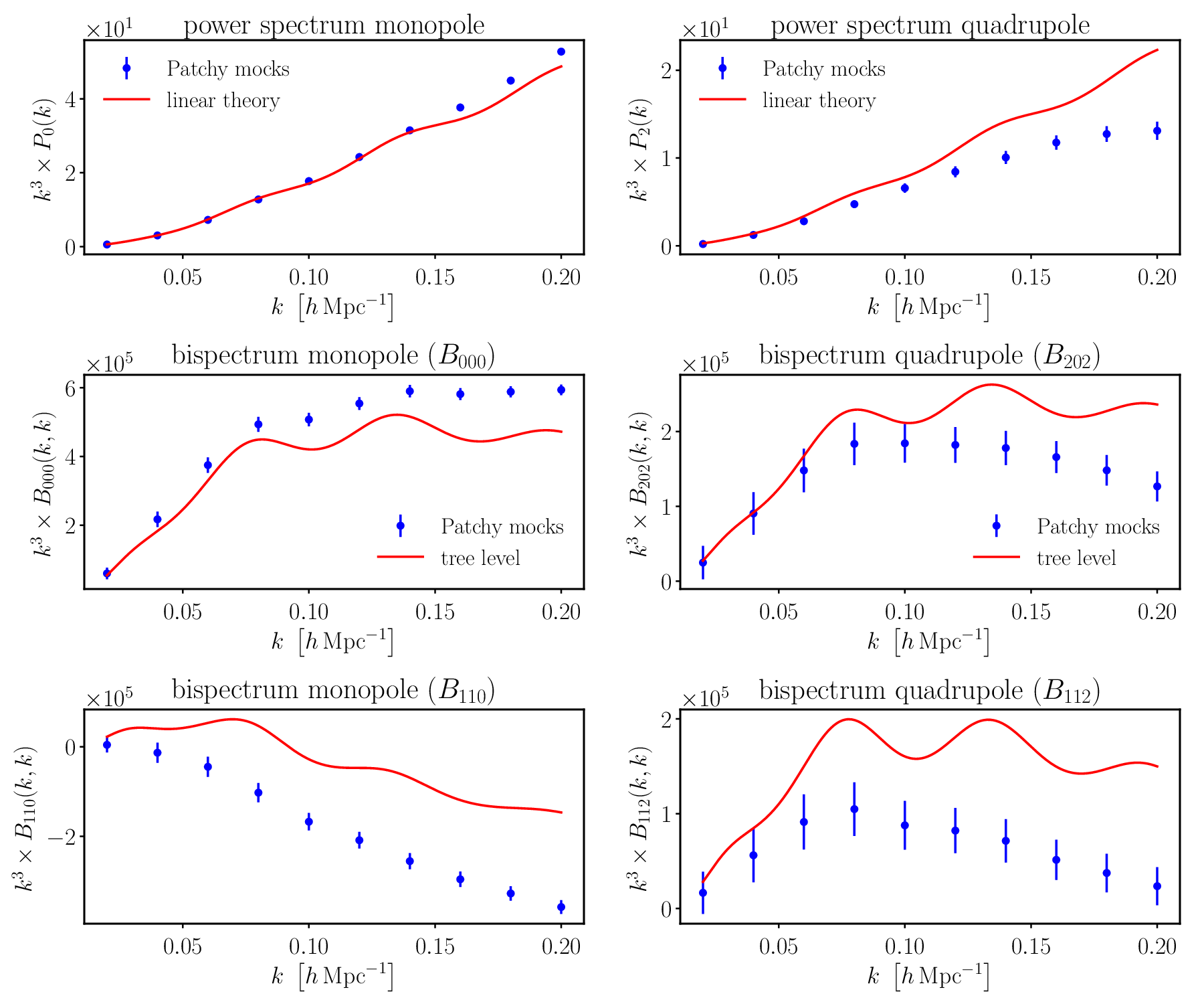
Refer to caption
Figure 8: Comparison of the power and bispectrum multipoles predicted using perturbation theory (red lines) with the corresponding measurements from the Patchy mocks (blue points).

In this appendix, we plot the power and bispectrum multipoles computed using perturbation theory (PT) at the leading order and compare them with the corresponding measurements from the Patchy mocks.

Figure 8 shows P0P_{0} (upper left), P2P_{2} (upper right), B000B_{000} (middle left), B202B_{202} (middle right), B110B_{110} (lower left) and B112B_{112} (lower right). For the monopole components of both the power and bispectra, P0P_{0}, B000B_{000} and B110B_{110}, the absolute values of their amplitudes computed by PT tend to be smaller than those of the Patchy mock measurements probably because of a lack of non-linear gravitational effects. On the other hand, for the quadrupole components, P2P_{2}, B202B_{202} and B112B_{112}, the Patchy mock results becomes smaller than the PT calculations on small scales probably due to non-linear velocity effects such as the Finger-of-God effect. For B110B_{110} and B112B_{112}, the PT solution starts to depart from the mock measurements even at larger scales k∼0.05​h​Mpc−1k\sim 0.05\,h\,{\rm Mpc^{-1}} compared to the scale for B000B_{000} and B202B_{202}, ∼0.1​h​Mpc−1\sim 0.1\,h\,{\rm Mpc^{-1}}. This may be because of lack of non-linear bias effects. Investigating the impact on the non-linear bias effect on the bispectrum signal and the corresponding covariance is left for future work.