Nucleon’s energy-momentum tensor form factors in light-cone QCD
Abstract
We use the energy-momentum tensor (EMT) current to compute the EMT form factors of the nucleon in the framework of the light cone QCD sum rule formalism. In the calculations, we employ the most general form of the nucleon’s interpolating field and use the distribution amplitudes (DAs) of the nucleon with two sets of the numerical values of the main input parameters entering the expressions of the DAs. The directly obtained results from the sum rules for the form factors are reliable at GeV2: To extrapolate the results to include the zero momentum transfer squared with the aim of estimation of the related static physical quantities, we use some fit functions for the form factors. The numerical computations show that the energy-momentum tensor form factors of the nucleon can be well fitted to the multipole fit form. We compare the results obtained for the form factors at with the existing theoretical predictions as well as experimental data on the gravitational form factor d. For the form factors M and J a consistency among the theoretical predictions is seen within the errors: Our results are nicely consistent with the Lattice QCD and chiral perturbation theory predictions. However, there are large discrepancies among the theoretical predictions on d. Nevertheless, our prediction is in accord with the JLab data as well as with the results of the Lattice QCD, chiral perturbation theory and KM15-fit. Our fit functions well define most of the JLab data in the interval GeV2, while the Lattice results suffer from large uncertainties in this region. As a by-product, some mechanical properties of the nucleon like the pressure and energy density at the center of nucleon as well as its mechanical radius are also calculated and their results are compared with other existing theoretical predictions.
Keywords:
Energy-momentum tensor form factors, nucleon DAs, Light-cone QCD sum rulesI Motivation
Understanding of the inner structures of the nucleons based on the quarks and gluons degrees of freedom is one of the most prominent research subjects of the hadron physics. A powerful instrument to probe the nucleon’s structure is to investigate the various form factors (FFs) of the nucleon as they carry direct information on the nucleon’ substructure and geometric shape. Indeed, the electromagnetic FFs of the nucleon unveil the way of distributions of the charge and magnetization of quarks inside the nucleon. The scalar and axial-vector FFs encompasses information on specific viewpoints of the nucleon’s substructure nature such as chiral and flavor symmetries and their breakdown. For these reasons, extensive research has been carried out on different form factors of the nucleon for decades. However, the gravitational or energy-momentum tensor form factors (EMTFFs) of the nucleon have recently been received considerable attention both in theory and experiment, despite they were recommended by Pagels in 1966 Pagels 1966. These form factors cannot be extracted directly from the experiment: They can be obtained from hard exclusive reactions using the Mellin moments of certain generalized parton distributions (GPDs). These form factors give us a tool for systematic studies of the properties of the nucleon and calculate different related observables like energy, angular momentum and pressure distributions inside the nucleon, etc.
The matrix element of the EMT current between the nucleon states is characterized by four form factors and parametrized as follows Ji 1997; Polyakov 2003
| (1) | |||||
where , , , and is the spinor of the nucleon with mass . Here, , , and are the EMTFFs of the nucleon. The form factor gives knowledge on the fractions of the momenta carried by the quark and gluon constituents of the nucleon. It is also related to the energy density distribution inside the nucleon. The form factor gives instruction about how the total angular momenta of quarks and gluons form the nucleon’s spin. The third form factor, (called the D-term), provides information on the distribution and stabilization of strong force in the nucleon. It can be obtained by the beam charge asymmetry in deeply virtual Compton scattering (DVCS). The negative sign of this form factor at zero-momentum transfer obtained from various theoretical studies is thought to be in connection with the spontaneous chiral symmetry breaking Polyakov and Weiss 1999; Kivel et al. 2001; Goeke et al. 2001; Jung et al. 2014a. The quark and gluon parts of the EMT current are not conserved separately, but their sum is conserved. The form factor characterizes the order of the non-conservation of the quark part of EMT current. This form factor is substantial to specify the distributions of the pressure forces inside the nucleon separately for quarks and gluons. This is also used to study the forces among quarks and gluons inside the nucleon. Hence, the EMTFFs provide new perspectives to the internal structure of the nucleon. More details can be found in a recent paper Polyakov and Schweitzer 2018.
The EMTFFs of the nucleon have been investigated in the framework of Lattice QCD Hagler et al. 2003; Mathur et al. 2000; Gockeler et al. 2004; Bratt et al. 2010; Hagler et al. 2008; Brommel et al. 2007; Negele et al. 2004; Deka et al. 2015, chiral perturbation theory (PT) Chen and Ji 2002; Belitsky and Ji 2002; Ando et al. 2006; Diehl et al. 2006; Diehl et al. 2007; Dorati et al. 2008, instant and front form (IFF) Lorcé et al. 2019, Skyrme model Cebulla et al. 2007; Kim et al. 2012, chiral quark soliton model (QSM) Petrov et al. 1998; Schweitzer et al. 2002; Ossmann et al. 2005; Wakamatsu and Tsujimoto 2005; Wakamatsu and Nakakoji 2006; Goeke et al. 2007a; Goeke et al. 2007b; Jung et al. 2014b; Jung et al. 2014a; Jung et al. 2016; Wakamatsu 2007, light-cone QCD sum rules at leading order(LCSR-LO) Anikin 2019, dispersion relation (DR) Pasquini et al. 2014 and instanton picture (IP) Polyakov and Son 2018. In Ref. Hagler et al. 2003, Hagler et al. calculated the quark part of the EMTFFs of the nucleon by means of the Lattice QCD. They obtained and at re-normalization scale of = 4 GeV2. In Ref. Mathur et al. 2000, Mathur et al. calculated the quark total angular momentum of the nucleon from the quark EMTFFs on the Lattice QCD and they found at re-normalization scale of = 1.74 GeV. In Ref. Gockeler et al. 2004, Gockeler et al. performed a quenched Lattice computation of the first moment of twist-two GPDs of the proton, and assessed the total quark contribution to the spin of the proton. They obtained , and at re-normalization scale of = 2 GeV. In Ref. Bratt et al. 2010, Bratt et al. presented their predictions for the substructure of the nucleon from a mixed-action computation using 2+1 flavors of asqtad sea and domain wall valence fermions. They carried out extrapolations of their data based on various chiral effective field theory pattern at re-normalization scale of = 4 GeV2. In Ref. Hagler et al. 2008 Hagler et al. presented a exhaustive study of the lowest moments of nucleon GPDs in 2 + 1 Lattice QCD by the help of domain wall valence quarks and refined staggered sea quarks without including the disconnected diagrams. They performed extrapolations of their results based on different chiral effective field theory schemes at re-normalization scale of = 4 GeV2. In Ref. Brommel et al. 2007, Brommel et al. reported on a calculation of nucleon’s GPDs based on simulations with two dynamical non-perturbatively improved Wilson quarks with pion masses down to 350 MeV. They found and at re-normalization scale of = 4 GeV2. In Ref. Deka et al. 2015, Deka et al. reported a comprehensive computation of the quark and gluon momenta in the nucleon. The computations encompass the contributions of quarks coming from both the connected and disconnected inclusions at re-normalization scale of = 2 GeV. In Ref. Dorati et al. 2008 Dorati et al. evaluated the basic properties related to the structures of baryons at low energies, by the help of the method of the covariant chiral perturbation theory in the baryon sector at leading-one-loop order. They investigated the quark-mass dependence of the isoscalar moments in the forward limit and estimated the contributions of quarks to the total spin of the nucleon at re-normalization scale of = 2 GeV. In Ref. Lorcé et al. 2019 Lorce et al. evaluated, in details, the distributions of energy, radial pressure and tangential pressure inside the nucleon in the framework of both the instant form and the front form of dynamics at re-normalization scale of = 2 GeV. In Ref. Anikin 2019 the author developed a method based on the light-cone sum rules at the leading order of to compute the gravitational form factors for the valence quark combinations in a nucleon at re-normalization scale of = 2 GeV2. In Refs. Cebulla et al. 2007; Kim et al. 2012, the EMTFFs of the nucleon are studied via the Skyrme and in-medium modified Skyrme models and they discuss how medium effects act on the form factors. In Refs. Petrov et al. 1998; Schweitzer et al. 2002; Ossmann et al. 2005; Wakamatsu and Tsujimoto 2005; Wakamatsu and Nakakoji 2006; Goeke et al. 2007a; Goeke et al. 2007b; Jung et al. 2014b; Jung et al. 2014a; Jung et al. 2016; Wakamatsu 2007, the EMTFFs of the nucleon are studied by means of the chiral quark-soliton model. It should be noted here that the Skyrme and QSM models show the total form factors which are re-normalization scale independent. In Ref. Pasquini et al. 2014, Pasquini et al. presented a depiction of the D-term form factor for hard exclusive reactions, making use of unsubtracted t-channel dispersion relations at re-normalization scale of = 4 GeV2. In Ref. Burkert et al. 2018, Burkert et al. presented an analysis of JLab data where an experimental information on the quark contribution to the D-term was obtained at re-normalization scale of = 1.5 GeV2. In Ref.Shanahan and Detmold 2019 the distributions of pressure and shear forces inside the proton are discussed via Lattice QCD computations of the EMTFFs at re-normalization scale of = 2 GeV.
In the present study, we compute the quark parts of the EMTFFs of the nucleon by the help of the light-cone QCD sum rules (LCSR) method, as one of the powerful and successful nonperturbative methods in hadron physics Braun and Filyanov 1989; Balitsky et al. 1989; Chernyak and Zhitnitsky 1990. The LCSR method is based on the operator product expansion (OPE) near the light-cone and expansion is carried out over the twists of the operators and the features of the hadrons under study are stated with respect to the features of the vacuum and the light-cone distribution amplitudes of the hadrons. Since the form factors are quantities with respect to the features of the vacuum and distribution amplitudes of the hadrons, any uncertainties in these parameters are reflected to the uncertainties of the estimations of the form factors. This method is quite accomplished in determining the baryonic form factors at high (see e.g. Aliev and Ozpineci 2006; Aliev and Savci 2007; Wang et al. 2006; Braun et al. 2006; Erkol and Ozpineci 2011a; Erkol and Ozpineci 2011b; Aliev et al. 2011; kucukarslan et al. 2016; Kucukarslan et al. 2016; Kucukarslan et al. 2014; Kucukarslan et al. 2015).
This manuscript is organized as follows. In section II, we formulate and derive the light-cone QCD sum rules for the nucleon EMTFFs. In section III, we present our numerical results for the nucleon EMTFFs. In section IV, we discuss the mechanical structure of the nucleon using the EMTFFs. Section V is reserved for the conclusions on the obtained results. The Appendices contain: a digression on alternative notations of the EMTFFs and technical details on the model expressions. A remark on different definitions and notations for the EMTFFs is given in Appendix A. The explicit expressions of the EMTFFs are moved to Appendix B.
II Formalism
In order to calculate the EMTFFs of the nucleon within LCSR, we begin our calculations with the subsequent correlation function:
| (2) |
where and is the energy-momentum tensor current. The quark and gluon parts of the EMT current are defined as
| (3) | |||||
| (4) |
The second part of Eq. (3) can be rewritten as Polyakov and Schweitzer 2018
| (5) |
where is the anomalous dimension of the mass operator. It should be noted here that we work in the chiral limit (). We also ignore the gluon fields contributions, i.e the gluonic part of the energy momentum tensor since taking into account these contributions requires knowledge of quark-gluon mixed distribution amplitudes of the nucleon which unfortunately are not available. Hence, in the present study, we will deal only with the first part of the quark part of the EMT current in Eq. (3). The covariant derivative is defined as ] with , ; and is the gluon field. In the correlation function above, is the nucleon’s interpolating current. In this study, we decide on the most general form of the interpolating current for nucleon, which is written as
| (6) |
where , , are the color indices, t is an arbitrary mixing parameter, and is the charge conjugation operator. Choosing reduces the above current to the famous Ioffe current.
In order to calculate sum rules for EMTFFs, we need to evaluate the correlator in two different languages. First, it is computed with respect to the QCD degrees of freedom: In terms of the parameters of the quarks and gluons and their non-perturbative interactions with the QCD vacuum.This representation is called the QCD or theoretical representation of the correlation function and it is obtained by the help of OPE in deep Euclidean space. In the second representation, the correlation function is calculated in terms of the hadronic parameters like the mass, residue, form factors and other hadronic degrees of freedom. This representation of the correlation function is called the physical or hadronic representation. Equating the coefficients of various Lorentz structures from two different representations of the same correlation function and carrying out a Borel transformation with the aim of eliminating the contributions of the continuum and higher states, we obtain sum rules for the EMTFFs of the nucleon. To further suppress the unwanted contributions and enhance the ground state contribution we apply the continuum subtraction procedure with accompany of the quark hadron duality assumption.
First we focus on the calculation of the hadronic side of the correlation function. To this end, we saturate the correlation function with a complete set of the nucleon state, the integration over four- leads to
| (7) |
where dots represent the unwanted contributions coming from the continuum and higher states. The above relation is further simplified by introducing the following definition:
| (8) |
where is the nucleon overlap amplitude or its residue. Inserting Eqs. (1) and (8) into Eq. (7), and performing summation over the spins of the Dirac spinors, we obtain the hadronic side of the correlation function in terms of the hadronic properties as well as different Lorentz structures as
| (9) |
On QCD side, we insert the explicit forms of the interpolating current for the nucleon and the EMT current into the correlation function and perform the required contractions using the Wick theorem. The resultant expression is in terms of the light quark propagator as well as the matrix elements of the quark fields sundwiched between the vacuum and nucleon states. The latter will be defined in terms of the nucleons DAs later. As a result we get
| (10) | |||||
where is the unit matrix and represents the up/down quark propagator which is given, in the limit , as
| (11) |
where, is the quark condensate and is specified with respect to the mixed quark-gluon condensate as . Since the expressions proportional to the gluon field strength tensor () are related to the four and five-particle distribution amplitudes, the contributions of these terms are expected to be small Diehl et al. 1999 and, therefore, these contributions will be neglected in our calculations. Furthermore, the terms proportional to are killed and they do not contribute after applying the Borel transformations. Hence, only the first term of the propagator survives in the calculations.
As it is clear from Eq. (10), to proceed in the calculations, we need to know the matrix elements of the quark operators sandwiched between the vacuum and nucleon states, i. e.
where , and are some real numbers. These matrix elements are parameterized in terms of the nucleon’s distributions amplitudes of different twists in the basis of the QCD conformal partial wave expansion approach Braun et al. 2006:
| (12) |
where is the spinor of the nucleon. The “calligraphic” functions, leaving aside the terms proportional to which contain , and , can be denoted in terms of the functions of the specific twist as:
where and are axialvector, pesudoscalar, scalar, tensor, and vector distribution amplitudes, respectively. The expansion of the matrix element is essentially an expansion in increasing twists of the distribution amplitudes. The distribution amplitudes , and have twist three, , , , , , , , and have twist 4, , , , , , , , and , are of twist 5, and , and functions have twist 6. The Baryon mass correction functions , and are also of twist 5. The distribution amplitudes , which are functions of , can be described as
| (13) |
where with are equivalent to the longitudinal momentum fractions carried by the quarks inside the nucleon. The explicit representations of the nucleon distribution amplitudes () can be found in Ref. Braun et al. 2006.
The desired LCSRs for the EMTFFs are acquired by matching the coefficients of various structures from both the hadronic and QCD sides of the correlation function in the momentum space. We use the structures , , and to find the sum rules for the form factors , , and , respectively. For the EMTFFs of the nucleon we obtain:
| (14) | ||||
| (15) | ||||
| (16) |
and
| (17) |
The explicit forms of the various functions that come into view in Eqs. (II) to (17) are presented in the Appendix with respect to the distribution amplitudes of the nucleon. For the sake of brevity, in the Appendix B, only the results for the form factor are presented, explicitly.
The last step is to apply the Borel transformation with respect to the variable as well as the continuum subtraction with the aim of suppression of the contributions of the higher states and continuum. These steps are performed by the help of the subsequent replacement rules (see e.g. Braun et al. 2006):
| (18) |
where,
| (19) |
is the Borel mass squared parameter and is the solution of the quadratic equation for :
| (20) |
with being the continuum threshold.
One of the main input parameters in the expressions of the sum rules for EMTFFs is the nucleon’s residue, . We use the expression of this parameter, in terms of the hadronic and QCD degrees of freedom as well as the auxiliary parameters entering the calculations, calculated via mass two-point sum rules Aliev et al. 2011. It is given as
| (21) |
where , and
III Numerical Results
The present section encompasses the numerical analyses of nucleon EMTFFs. In order to obtain the numerical results of the form factors, expressions of the distribution amplitudes for nucleon are needed. We borrow them from Ref. Braun et al. 2006. These distribution amplitudes include eight nonperturbative hadronic parameters, which are obtained in the framework of different models. In further numerical computations we take into account two different sets of these parameters: 1) QCD sum rules (QCDSR) based distribution amplitudes, where corrections to the distribution amplitudes are considered and the parameters in distribution amplitudes are obtained from QCDSR (Set-I), 2) The condition that the next to leading conformal spin contributions vanish, fixes five of the eight parameters, and remaining three parameters (, , ) are borrowed from QCDSR. This set is called asymptotic set (Set-II). The values of these parameters in two different sets are given in Table 1. In addition we use: , GeV, GeV3 and GeV2 Ioffe 2006.
There are three auxiliary parameters of the QCDSR to be fixed: the continuum threshold , the Borel mass parameter and the mixing parameter . The continuum threshold starts from the point, where the excited states and continuum contribute to the correlation function. We use the continuum threshold in the range GeV2, which is pretty much fixed in the literature from the nucleon spectrum analyses. The working region of is decided to be in the interval GeV2 GeV2. As it can be seen from Fig. 1 (as an example), the results of the form factors are roughly independent of the Borel parameter in the interval GeV2 GeV2. We include into the final results the errors coming from the variations of the physical observables with respect to the auxiliary parameters, which remain below the limits accepted by the sum rules computations. The next step is to specify the optimal mixing parameter . Our numerical calculations indicate that the form factors are not sensitive to cos (with tan) when it varies in the region -0.2 -0.4. We see that the famous Ioffe current for the nucleon, which corresponds to the choice cos remains out of the reliable the working region.


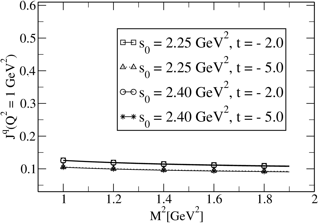


Figure 2 shows the changes of the energy-momentum tensor form factors of the nucleon with respect to the momentum transfer squared . As is also clear from this figure, the sum rules for the EMTFFs give reliable results for GeV2. To extrapolate the results to the smaller points as well as , which enables us to compute the static properties of the nucleon, we use some fit functions such that the results of fit functions coincide with the LCSRs predictions at the region GeV2. Our numerical computations show that, the EMTFFs of the nucleon can be well described by the multipole fit functions defined as Anikin 2019
| (22) |
| Results of set-I | Results of set-II | |||||||||
|---|---|---|---|---|---|---|---|---|---|---|
|
|
|
|
(GeV | p | |||||
| M | ||||||||||
| J | ||||||||||
| d | ||||||||||
The values of the fit parameters, i. e. the form factors at , and for different EMTFFs obtained from the sum rules analyses are shown in Table 2. The errors in the presented results are due to the variations in the computations of the working regions of , and mixing parameter as well as the uncertainties in the values of the input parameters and the nucleon distribution amplitudes. Although the central values of the form factors at obtained via two sets of distribution amplitudes differ slightly from each other but they are consistent within the presented errors.
The individual quark and gluon EMTFFs are not re-normalization scale independent. The numerical values of distribution amplitudes are used at the scale GeV2 in Ref. Chernyak and Zhitnitsky 1984. In the present study our estimations correspond to GeV2, as well. Different sources use different scales to calculate the EMTFFs. In order to compare the results, we should bring them in the same re-normalization scale. To this end, we use the evolution equations, for the form factors under consideration, calculated in Refs. Hatta et al. 2018; Tanaka 2019.


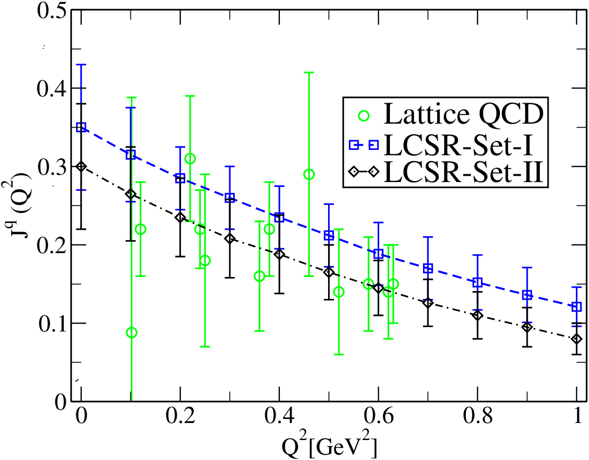

Table 3 displays a comparison of our results at with those of the various theoretical models, Lattice QCD and existing experimental data for d(0) at re-normalization scale GeV2. For the M form factor, almost all approaches give, more or less, similar predictions. For the J form factor, our estimations are in good agreements, within the errors, with the predictions of Refs. Lorcé et al. 2019; Hagler et al. 2003; Mathur et al. 2000; Gockeler et al. 2004; Bratt et al. 2010; Hagler et al. 2008; Brommel et al. 2007; Negele et al. 2004; Deka et al. 2015; Dorati et al. 2008. Note that in the QSM and Skyrme models 2 = 1, since there are only quarks and antiquarks to carry the nucleon’s angular momentum and they must carry 100 of it. Despite all of the results for d(0) from different sources have the same sign, there are large discrepancies among the results. Our predictions for both of the DAs are in accord with the JLab data. Our estimations are also consistent, within the errors, with the predictions of Refs. Lorcé et al. 2019; Hagler et al. 2008; Bratt et al. 2010; Dorati et al. 2008; Goeke et al. 2007b; Anikin 2019; Pasquini et al. 2014; Anikin et al. 2018, but they differ from the other predictions presented in the table. The negative sign of the d(0) form factor indicates a profound connection with the spontaneous chiral symmetry breaking in QCD (see also Polyakov and Weiss 1999; Kivel et al. 2001; Goeke et al. 2001) as well as an attractive relation with the criterion of stability of the nucleon Goeke et al. 2007b. The values obtained for the form factor using both of the DAs in the present study as well as the prediction of IP Polyakov and Son 2018 are quite small, telling us that the quark and gluon subsystems inside the nucleon interact weakly. Our predictions for , however, differ with the predictions of IFF Lorcé et al. 2019, substantially.
At the end of this section, we would like to compare the behaviors of the , and form factors at small values of with the Lattice predictions as well as JLab data for the gravitational form factor. To this end we plot Fig. 3. The Lattice data points in this figure are taken from the LHPC Collaboration Hagler et al. 2008 and the JLab data form Ref. Burkert et al. 2018. For the form factor , our predictions are consistent with most of the Lattice QCD data points considering the errorbars. In the case of and form factors the Lattice results suffer from large uncertainties at small values of . Our predictions, especially obtained via set-II DAs reproduce most of the JLab data at small values of . This can be considered as a good assurance for the behaviors of the EMTFFs with respect to at all regions and in particular at .
| Approaches | M(0) | Jq(0) | d(0) | |
|---|---|---|---|---|
| Lattice QCD Hagler et al. 2003 | 0.74 0.07 | 0.37 0.03 | - | - |
| Lattice QCD Mathur et al. 2000 | 0.62 0.14 | 0.31 0.07 | - | - |
| Lattice QCD Gockeler et al. 2004 | 0.72 0.14 | 0.36 0.08 | -1.09 0.06 | - |
| Lattice QCD Bratt et al. 2010 | 0.59 0.05 | 0.28 0.02 | -1.76 0.09 | - |
| Lattice QCD Hagler et al. 2008 | 0.53 0.02 | 0.28 0.02 | -2.27 0.30 | - |
| Lattice QCD Brommel et al. 2007 | 0.61 0.15 | 0.24 0.06 | - | - |
| Lattice QCD Negele et al. 2004 | 0.74 0.07 | 0.37 0.03 | - | - |
| Lattice QCD Deka et al. 2015 | 0.75 0.07 | 0.38 0.04 | - | - |
| PT Dorati et al. 2008 | 0.57 0.04 | 0.25 0.06 | -1.93 0.06 | - |
| IFF Lorcé et al. 2019 | 0.58 | 0.25 | -1.92 | -0.11 |
| Skyrme Cebulla et al. 2007 | 1 | 0.5 | -4.48 | - |
| Skyrme Kim et al. 2012 | 1 | 0.5 | -3.54 | - |
| QSM Goeke et al. 2007b | 1 | 0.5 | -2.35 | - |
| QSM Jung et al. 2014a | 1 | 0.5 | -5.03 | |
| QSM Wakamatsu 2007 | - | - | -4.85 | - |
| LCSR-LO Anikin 2019 | - | - | -2.63 0.22 | - |
| KM15 fit Anikin et al. 2018 | - | - | -2.18 0.21 | - |
| DR Pasquini et al. 2014 | - | - | -1.70 | - |
| JLab data Burkert et al. 2018 | - | - | - | |
| IP Polyakov and Son 2018 | - | - | - | |
| This Work (Set-I) | 0.79 0.10 | 0.36 0.10 | -2.29 0.58 | |
| This Work (Set-II) | 0.74 0.12 | 0.30 0.11 | -2.05 0.40 |
IV Mechanical Properties of Nucleon
Having calculated the energy-momentum tensor form factors, it is straightforward to calculate the pressure and the energy density at the center of nucleon as well as estimate the hadron mechanical radius. The related formulas for and are given as Polyakov and Schweitzer 2018:
| (23) | |||||
| (24) |
where . Our results on the mechanical quantities and of the nucleon compared to other existing theoretical predictions are shown in table 4. One can see from Table 4 that our predictions on , within the errors, are very close to that of Jung et al. 2014a, however, they differ with other predictions, considerably. Our results on using both sets of DAs are close to the predictions of Kim et al. 2012 and Goeke et al. 2007b, but demonstrate considerable deviations from other presented predictions. We should remind that , in the case one considers both the gluonic and quark parts of the energy-momentum tensor, implying that the energy-momentum tensor current is conserved. However, as we previously mentioned we obtained very small values for the form factor at different points, referring to a very small violation of the current conservation. These small values for do not affect the mechanical properties. We shall also note that the quantity has very small impact on the , a result that also is found in Polyakov and Schweitzer 2018. Ignoring , for the mechanical mean squre radius, one obtains Polyakov and Schweitzer 2018
| (25) |
The numerical results for , using two sets of DAs, compared to the only existing prediction from Ref. Anikin 2019 are shown in table 4, as well. As it is seen, our predictions on using both sets are in good consistencies with the prediction of Ref. Anikin 2019 within the presented uncertainties. The presented results and their comparison with probable future experimental data can be very useful in understanding the structure of the nucleon.
| Mechanical properties | Results of set-I | Results of set-II | Cebulla et al. 2007 | Kim et al. 2012 | Goeke et al. 2007b | Jung et al. 2014a | Anikin 2019 |
|---|---|---|---|---|---|---|---|
| (GeV/fm3) | 0.47 | 0.26 | 0.23 | 0.58 | 0.86 | ||
| (GeV/fm3) | 2.28 | 1.45 | 1.70 | 3.56 | 0.94 | ||
| (fm2) | - | - | - | - | 0.54 |
V Summary and Concluding Remarks
The energy-momentum tensor or gravitational form factors of nucleon are basic quantities that carry valuable information on different aspects of the nucleon’s structure. These are used to calculate the pressure and energy distributions inside the nucleon as well as quantities related to its geometric shape. The EMTFFs are also sources of information on the fractions of the momenta carried by the quarks and gluons as ingredients of the nucleon. They help us know how the total angular momenta of quarks and gluons form the nucleon’s spin. They also provide knowledge on the distribution and stabilization of the strong force inside the nucleon. We extracted the EMTFFs of the nucleon by applying the light-cone QCD sum rule formalism and using two different sets of the parameters inside the nucleon’s distribution amplitudes. In the calculations, we used the most general interpolating current of the nucleon in terms of its constituent quark fields. We observed that the results don’t depend on the choice of the DAs, considerably and the two sets give close results to each other. We found that the EMTFFs of nucleon are best described by a multipole fit function, helped us to extrapolate the results to the regions that the LCSRs results are not reliable and applicable.
We extracted the numerical values of the EMTFFs at and compared the results with the existing theoretical predictions as well as the results of the Lattice QCD and JLab data. We observed a consistency among the theoretical predictions, within the uncertainties, for the values of the form factors M and J. Our results on these form factors are nicely consistent with the Lattice QCD and chiral perturbation theory predictions. However, there are large discrepancies among the theoretical predictions on the gravitational form factor d. Nevertheless, our prediction is in accord with the JLab data as well as with the predictions of the Lattice QCD, chiral perturbation theory and KM15-fit. We obtained a very small value for the form factor referring to a good conservation of the quark part of the EMT current.
We discussed the behavior of the EMTFFs with respect to and observed that all form factors approach to zero at large values of . Making use of the multipole fit function, we glanced the behavior of the FFs at small values of , where we have some experimental data on d provided by JLab. We saw that the fit function considered in the present study well defines most of the JLab data in the interval . The Lattice QCD results for d and J suffer from large uncertainties in this region. The behaviors of the form factor M obtained using two sets of DAs in the present study are consistent with the Lattice QCD predictions that contain small uncertainties at small values of .
Making use of the fit functions of the form factors, we calculated the pressure and energy density distributions at the center of nucleon as well as the mechanical radius of the nucleon and compared with the existing theoretical predictions. Our predictions on , using two sets of DAs, are very close to that of QSM Jung et al. 2014a within the errors, however, they differ with other predictions presented in table 4, considerably. Our predictions on at the center of the nucleon are close to the predictions of Skyrme modelKim et al. 2012 and QSM Goeke et al. 2007b, but demonstrate considerable deviations from other presented predictions. The predictions of the present study on are in good consistencies with the only existing prediction provided by LCSR-LO approach Anikin 2019 within the presented uncertainties.
The presented results in this study together with the predictions of Lattice QCD and other theoretical predictions on the nucleon’s EMTFFs may help experimental groups to measure the values of these form factors at a wide range of . The good consistency between our predictions and the existing JLab data on d in the interval GeV2, strengthens this hope. Any experimental data on the energy momentum tensor as well as the electromagnetic, axial and other form factors of the nucleon and their comparison with the theoretical predictions can help us gain valuable knowledge on the internal structures and geometric shapes of the nucleons as building blocks of the visible matter. Such investigations may also help us answer many fundamental questions by means of the quark-gluon structures of the nucleons.
VI Acknowledgements
U. Ö. thanks the scientific and technological research council of Turkey (TUBITAK) for the support provided under 2218-National Postdoctoral Research Scholarship Program.
Appendix A Alternative definition of the EMT current’s matrix element
Appendix B Explicit forms of the F functions for the form factor
References
- Pagels (1966) H. Pagels, Phys. Rev. 144, 1250 (1966).
- Ji (1997) X.-D. Ji, Phys. Rev. Lett. 78, 610 (1997), arXiv:hep-ph/9603249 [hep-ph] .
- Polyakov (2003) M. V. Polyakov, Phys. Lett. B555, 57 (2003), arXiv:hep-ph/0210165 [hep-ph] .
- Polyakov and Weiss (1999) M. V. Polyakov and C. Weiss, Phys. Rev. D60, 114017 (1999), arXiv:hep-ph/9902451 [hep-ph] .
- Kivel et al. (2001) N. Kivel, M. V. Polyakov, and M. Vanderhaeghen, Phys. Rev. D63, 114014 (2001), arXiv:hep-ph/0012136 [hep-ph] .
- Goeke et al. (2001) K. Goeke, M. V. Polyakov, and M. Vanderhaeghen, Prog. Part. Nucl. Phys. 47, 401 (2001), arXiv:hep-ph/0106012 [hep-ph] .
- Jung et al. (2014a) J.-H. Jung, U. Yakhshiev, H.-C. Kim, and P. Schweitzer, Phys. Rev. D89, 114021 (2014a), arXiv:1402.0161 [hep-ph] .
- Polyakov and Schweitzer (2018) M. V. Polyakov and P. Schweitzer, Int. J. Mod. Phys. A33, 1830025 (2018), arXiv:1805.06596 [hep-ph] .
- Hagler et al. (2003) P. Hagler, J. W. Negele, D. B. Renner, W. Schroers, T. Lippert, and K. Schilling (LHPC, SESAM), Phys. Rev. D68, 034505 (2003), arXiv:hep-lat/0304018 [hep-lat] .
- Mathur et al. (2000) N. Mathur, S. J. Dong, K. F. Liu, L. Mankiewicz, and N. C. Mukhopadhyay, Phys. Rev. D62, 114504 (2000), arXiv:hep-ph/9912289 [hep-ph] .
- Gockeler et al. (2004) M. Gockeler, R. Horsley, D. Pleiter, P. E. L. Rakow, A. Schafer, G. Schierholz, and W. Schroers (QCDSF), Phys. Rev. Lett. 92, 042002 (2004), arXiv:hep-ph/0304249 [hep-ph] .
- Bratt et al. (2010) J. D. Bratt et al. (LHPC), Phys. Rev. D82, 094502 (2010), arXiv:1001.3620 [hep-lat] .
- Hagler et al. (2008) P. Hagler et al. (LHPC), Phys. Rev. D77, 094502 (2008), arXiv:0705.4295 [hep-lat] .
- Brommel et al. (2007) D. Brommel et al. (QCDSF-UKQCD), Proceedings, 25th International Symposium on Lattice field theory (Lattice 2007): Regensburg, Germany, July 30-August 4, 2007, PoS LATTICE2007, 158 (2007), arXiv:0710.1534 [hep-lat] .
- Negele et al. (2004) J. W. Negele et al., Lattice hadron physics. Proceedings, 2nd Topical Workshop, LHP 2003, Cairns, Australia, July 22-30, 2003, Nucl. Phys. Proc. Suppl. 128, 170 (2004), [,170(2004)], arXiv:hep-lat/0404005 [hep-lat] .
- Deka et al. (2015) M. Deka et al., Phys. Rev. D91, 014505 (2015), arXiv:1312.4816 [hep-lat] .
- Chen and Ji (2002) J.-W. Chen and X.-d. Ji, Phys. Rev. Lett. 88, 052003 (2002), arXiv:hep-ph/0111048 [hep-ph] .
- Belitsky and Ji (2002) A. V. Belitsky and X. Ji, Phys. Lett. B538, 289 (2002), arXiv:hep-ph/0203276 [hep-ph] .
- Ando et al. (2006) S.-i. Ando, J.-W. Chen, and C.-W. Kao, Phys. Rev. D74, 094013 (2006), arXiv:hep-ph/0602200 [hep-ph] .
- Diehl et al. (2006) M. Diehl, A. Manashov, and A. Schafer, Eur. Phys. J. A29, 315 (2006), arXiv:hep-ph/0608113 [hep-ph] .
- Diehl et al. (2007) M. Diehl, A. Manashov, and A. Schafer, Eur. Phys. J. A31, 335 (2007), arXiv:hep-ph/0611101 [hep-ph] .
- Dorati et al. (2008) M. Dorati, T. A. Gail, and T. R. Hemmert, Nucl. Phys. A798, 96 (2008), arXiv:nucl-th/0703073 [nucl-th] .
- Lorcé et al. (2019) C. Lorcé, H. Moutarde, and A. P. Trawiński, Eur. Phys. J. C79, 89 (2019), arXiv:1810.09837 [hep-ph] .
- Cebulla et al. (2007) C. Cebulla, K. Goeke, J. Ossmann, and P. Schweitzer, Nucl. Phys. A794, 87 (2007), arXiv:hep-ph/0703025 [HEP-PH] .
- Kim et al. (2012) H.-C. Kim, P. Schweitzer, and U. Yakhshiev, Phys. Lett. B718, 625 (2012), arXiv:1205.5228 [hep-ph] .
- Petrov et al. (1998) V. Yu. Petrov, P. V. Pobylitsa, M. V. Polyakov, I. Bornig, K. Goeke, and C. Weiss, Phys. Rev. D57, 4325 (1998), arXiv:hep-ph/9710270 [hep-ph] .
- Schweitzer et al. (2002) P. Schweitzer, S. Boffi, and M. Radici, Phys. Rev. D66, 114004 (2002), arXiv:hep-ph/0207230 [hep-ph] .
- Ossmann et al. (2005) J. Ossmann, M. V. Polyakov, P. Schweitzer, D. Urbano, and K. Goeke, Phys. Rev. D71, 034011 (2005), arXiv:hep-ph/0411172 [hep-ph] .
- Wakamatsu and Tsujimoto (2005) M. Wakamatsu and H. Tsujimoto, Phys. Rev. D71, 074001 (2005), arXiv:hep-ph/0502030 [hep-ph] .
- Wakamatsu and Nakakoji (2006) M. Wakamatsu and Y. Nakakoji, Phys. Rev. D74, 054006 (2006), arXiv:hep-ph/0605279 [hep-ph] .
- Goeke et al. (2007a) K. Goeke, J. Grabis, J. Ossmann, P. Schweitzer, A. Silva, and D. Urbano, Phys. Rev. C75, 055207 (2007a), arXiv:hep-ph/0702031 [HEP-PH] .
- Goeke et al. (2007b) K. Goeke, J. Grabis, J. Ossmann, M. V. Polyakov, P. Schweitzer, A. Silva, and D. Urbano, Phys. Rev. D75, 094021 (2007b), arXiv:hep-ph/0702030 [hep-ph] .
- Jung et al. (2014b) J.-H. Jung, U. Yakhshiev, and H.-C. Kim, J. Phys. G41, 055107 (2014b), arXiv:1310.8064 [hep-ph] .
- Jung et al. (2016) J.-H. Jung, U. Yakhshiev, and H.-C. Kim, Phys. Rev. D93, 054016 (2016), arXiv:1512.07378 [hep-ph] .
- Wakamatsu (2007) M. Wakamatsu, Phys. Lett. B648, 181 (2007), arXiv:hep-ph/0701057 [hep-ph] .
- Anikin (2019) I. V. Anikin, Phys. Rev. D99, 094026 (2019), arXiv:1902.00094 [hep-ph] .
- Pasquini et al. (2014) B. Pasquini, M. V. Polyakov, and M. Vanderhaeghen, Phys. Lett. B739, 133 (2014), arXiv:1407.5960 [hep-ph] .
- Polyakov and Son (2018) M. V. Polyakov and H.-D. Son, JHEP 09, 156 (2018), arXiv:1808.00155 [hep-ph] .
- Burkert et al. (2018) V. D. Burkert, L. Elouadrhiri, and F. X. Girod, Nature 557, 396 (2018).
- Shanahan and Detmold (2019) P. E. Shanahan and W. Detmold, Phys. Rev. Lett. 122, 072003 (2019), arXiv:1810.07589 [nucl-th] .
- Braun and Filyanov (1989) V. M. Braun and I. E. Filyanov, Z. Phys. C44, 157 (1989), [Yad. Fiz.50,818(1989)].
- Balitsky et al. (1989) I. I. Balitsky, V. M. Braun, and A. V. Kolesnichenko, Nucl. Phys. B312, 509 (1989).
- Chernyak and Zhitnitsky (1990) V. L. Chernyak and I. R. Zhitnitsky, Nucl. Phys. B345, 137 (1990).
- Aliev and Ozpineci (2006) T. M. Aliev and A. Ozpineci, Nucl. Phys. B732, 291 (2006), arXiv:hep-ph/0406331 [hep-ph] .
- Aliev and Savci (2007) T. M. Aliev and M. Savci, Phys. Lett. B656, 56 (2007), arXiv:0711.1757 [hep-ph] .
- Wang et al. (2006) Z.-G. Wang, S.-L. Wan, and W.-M. Yang, Eur. Phys. J. C47, 375 (2006), arXiv:hep-ph/0601060 [hep-ph] .
- Braun et al. (2006) V. M. Braun, A. Lenz, and M. Wittmann, Phys. Rev. D73, 094019 (2006), arXiv:hep-ph/0604050 [hep-ph] .
- Erkol and Ozpineci (2011a) G. Erkol and A. Ozpineci, Phys. Lett. B704, 551 (2011a), arXiv:1107.4584 [hep-ph] .
- Erkol and Ozpineci (2011b) G. Erkol and A. Ozpineci, Phys. Rev. D83, 114022 (2011b), arXiv:1105.1637 [hep-ph] .
- Aliev et al. (2011) T. M. Aliev, K. Azizi, and M. Savci, Phys. Rev. D84, 076005 (2011), arXiv:1108.2019 [hep-ph] .
- kucukarslan et al. (2016) A. kucukarslan, U. Ozdem, and A. Ozpineci, Phys. Rev. D94, 094010 (2016), arXiv:1610.08358 [hep-ph] .
- Kucukarslan et al. (2016) A. Kucukarslan, U. Ozdem, and A. Ozpineci, Nucl. Phys. B913, 132 (2016), arXiv:1512.01015 [hep-ph] .
- Kucukarslan et al. (2014) A. Kucukarslan, U. Ozdem, and A. Ozpineci, Phys. Rev. D90, 054002 (2014), arXiv:1407.3735 [hep-ph] .
- Kucukarslan et al. (2015) A. Kucukarslan, U. Ozdem, and A. Ozpineci, J. Phys. G42, 015001 (2015), arXiv:1405.5339 [hep-ph] .
- Diehl et al. (1999) M. Diehl, T. Feldmann, R. Jakob, and P. Kroll, Eur. Phys. J. C8, 409 (1999), arXiv:hep-ph/9811253 [hep-ph] .
- Ioffe (2006) B. L. Ioffe, Prog. Part. Nucl. Phys. 56, 232 (2006), arXiv:hep-ph/0502148 [hep-ph] .
- Chernyak and Zhitnitsky (1984) V. L. Chernyak and I. R. Zhitnitsky, Nucl. Phys. B246, 52 (1984).
- Hatta et al. (2018) Y. Hatta, A. Rajan, and K. Tanaka, JHEP 12, 008 (2018), arXiv:1810.05116 [hep-ph] .
- Tanaka (2019) K. Tanaka, JHEP 01, 120 (2019), arXiv:1811.07879 [hep-ph] .
- Anikin et al. (2018) I. V. Anikin et al., Acta Phys. Polon. B49, 741 (2018), arXiv:1712.04198 [nucl-ex] .