Chapter 3
-adic sequences.
A bridge between dynamics, arithmetic, and geometry
Abstract.
A Sturmian sequence is an infinite nonperiodic string over two letters with minimal subword complexity. In two papers, the first written by Morse and Hedlund in 1940 and the second by Coven and Hedlund in 1973, a surprising correspondence was established between Sturmian sequences on one side and rotations by an irrational number on the unit circle on the other. In 1991 Arnoux and Rauzy observed that an induction process (invented by Rauzy in the late 1970s), related with the classical continued fraction algorithm, can be used to give a very elegant proof of this correspondence. This process, known as the Rauzy induction, extends naturally to interval exchange transformations (this is the setting in which it was first formalized). It has been conjectured since the early 1990s that these correspondences carry over to rotations on higher dimensional tori, generalized continued fraction algorithms, and so-called -adic sequences generated by substitutions. The idea of working towards such a generalization is known as Rauzy’s program. Recently Berthé, Steiner, and Thuswaldner made some progress on Rauzy’s program and were indeed able to set up the conjectured generalization of the above correspondences. Using a generalization of Rauzy’s induction process in which generalized continued fraction algorithms show up, they proved that under certain natural conditions an -adic sequence gives rise to a dynamical system which is measurably conjugate to a rotation on a higher dimensional torus. Moreover, they established a metric theory which shows that counterexamples like the one constructed in 2000 by Cassaigne, Ferenczi, and Zamboni are rare. It is the aim of the present chapter to survey all these ideas and results.
Chapter 3
3.1. Introduction
A Sturmian sequence is an infinite string over two letters with low subword complexity. In particular, it has exactly different subwords of a given length . Sturmian sequences have been studied extensively in the literature from various points of view and we refer to Lothaire [101, Chapter 2] or Pytheas Fogg [82, Chapter 6] for detailed accounts. The history of the research surveyed in the present chapter starts with two papers written by Morse and Hedlund [107] as well as Coven and Hedlund [67] in 1940 and 1973, respectively. In these papers the authors established a surprising correspondence between Sturmian sequences and rotations by an irrational number on the torus . In their proof “balance properties” of Sturmian sequences play a prominent role. Several decades later, Arnoux and Rauzy [22] observed that an induction process in which the classical continued fraction algorithm appears can be used to give another very elegant proof of this correspondence (see also Rauzy’s earlier papers [112, 113] on this induction process). Their proof also shows how arithmetic and Diophantine properties of an irrational number are encoded in the corresponding Sturmian sequence.
It has been conjectured since the early 1990s that these correspondences between rotations on , continued fractions, and Sturmian sequences carry over to rotations on higher dimensional tori, generalized continued fraction algorithms, and so-called -adic sequences generated by substitutions. The idea of working towards such a generalization is known as Rauzy’s program and starting with Rauzy [114] a number of examples which hint at such a generalization was devised. A natural class of -adic sequences to study in this context are so-called Arnoux-Rauzy sequences which go back to Arnoux and Rauzy [22]. These are sequences over three letters that behave analogously to Sturmian sequences in many regards. However, in 2000 Cassaigne, Ferenczi, and Zamboni [63] could construct Arnoux-Rauzy sequences with strong “imbalance”, a property which cannot occur for a Sturmian sequence. Cassaigne, Ferenczi, and Messaoudi [62] even constructed Arnoux-Rauzy sequences that give rise to weakly-mixing dynamical systems which are far from rotations in their dynamical behavior. All this shows the limitations of Rauzy’s program and indicates that the situation in the general setting is more complicated than it is in the classical case.
Nevertheless, recently Berthé, Steiner, and Thuswaldner [52] made some progress on Rauzy’s program and were indeed able to set up the conjectured generalization of the above correspondences. Using a generalization of Rauzy’s induction process in which generalized continued fraction algorithms show up, they proved that under certain natural conditions an -adic sequence gives rise to a dynamical system which is measurably conjugate to a rotation on a higher dimensional torus. Moreover, they established a metric theory which shows that exceptional cases like the ones constructed in [62] and [63] are rare. A prominent role in this generalization is played by tilings induced by generalizations of the classical Rauzy fractal introduced by Rauzy [114].
Another idea which can be linked to the above results goes back to Artin [26], who observed that the classical continued fraction algorithm and its natural extension can be viewed as a Poincaré section of the geodesic flow on the space of two-dimensional lattices . Arnoux and Fisher [14] revisited Artin’s idea and showed that the correspondence between continued fractions, rotations, and Sturmian sequences can be interpreted in a very nice way in terms of an extension of this geodesic flow to pointed lattices which is called the scenery flow. Currently, Arnoux et al. [12] are setting up a generalization of this connection between continued fraction algorithms and geodesic flows. In particular, they code the Weyl Chamber Flow, a diagonal -action on the space of -dimensional lattices , arithmetically and geometrically by generalized continued fraction algorithms. In this coding, which provides a new view of the relation between -adic sequences and rotations on higher dimensional tori, non-stationary Markov partitions defined in terms of generalized Rauzy fractals are of great importance.
It is the aim of the present chapter to survey all these ideas and results. In Section 3.2 we deal with the case of Sturmian sequences and Section 3.3 discusses the problems with the extension of the theory to the more general situation. From Section 3.4 onwards we set up the general theory of -adic sequences and their relation to generalized continued fraction algorithms and rotations on higher dimensional tori.
3.2. The classical case
We start our journey by giving some elements of the interaction between Sturmian sequences, the classical continued fraction algorithm, and irrational rotations on the circle. After that we discuss natural extensions of continued fractions and show how all these objects turn up in the study of the geodesic flow acting on the space of lattices and its extension to pointed lattices. We will prove most of the results that we state and although our exposition is self-contained we recommend the reader to have a look at the survey [82, Chapter 6] in order to find more background information on the subject of this section.
3.2.1. Sturmian sequences and their basic properties
For a finite set denote by the set of all finite words whose letters , , are contained in . Moreover, let be the space of (right-infinite) sequences whose letters , , are elements of . The shift on this space of sequences is defined by Let be a sequence. A factor (or subword) of is a word for which there is such that . In this case we say that occurs in at position . The complexity function of assigns to each integer the number of words that are factors of . If is ultimately periodic in the sense that there exist and with for each then is a bounded function. On the other hand, a result by Coven and Hedlund [67] which is not hard to prove states that a sequence that admits the inequality for a single choice of is ultimately periodic (see also [82, Proposition 1.1.1]). It is the class of not ultimately periodic sequences with smallest complexity function that we are interested in.
Definition 3.2.1 (Sturmian sequence).
A sequence is called a Sturmian sequence if its complexity function satisfies for all .
It is a priori not clear that Sturmian sequences exist at all. However, we will see in Theorem 3.2.11 below that they can be characterized as so-called natural codings of irrational rotations which are easy to construct (and will be defined in Section 3.2.4).
A detailed account on the early history of Sturmian sequences, which goes back to Johann Bernoulli [39], is given in [101, Notes to Chapter 2]. The name “Sturmian sequence” was coined in 1940 by Morse and Hedlund [107]. Sturmian sequences have been studied extensively. For an overview on fundamental properties of Sturmian sequences we refer in particular to Lothaire [101, Chapter 2], Pytheas Fogg [82, Chapter 6], or Allouche and Shallit [6, Chapters 9 and 10]. Belov et al. [38] discuss some aspects of Sturmian sequences which are related to the present survey.
We start with the discussion of basic properties of Sturmian sequences. The fact that holds for a Sturmian sequence entails that for each there is only one factor of with the property that both words and are factors of . Such a word is called right special factor of . Left special factors are defined analogously.
Our first lemma deals with recurrence of Sturmian sequences. Recall that a sequence is called recurrent if each factor of occurs infinitely often, i.e., at infinitely many positions, in .
Lemma 3.2.2 (cf. e.g. [82, Proposition 6.1.2]).
A Sturmian sequence is recurrent.
Proof.
Suppose that this is wrong and let be a nonrecurrent Sturmian sequence. Then there exists a factor of length , say, that occurs only finitely many times in . Then there exists such that does not contain as a factor. However, as this implies that and, hence, is ultimately periodic. However, then also is ultimately periodic, a contradiction. ∎
Next we discuss balance. To give a formal definition we introduce some notation. For a word we denote by its length, i.e., the number of letters of . Moreover, for , we write for the number of occurrences of the letter in .
Definition 3.2.3 (Balanced sequence).
A sequence is called balanced if each pair of factors of with satisfies .
As was observed already in [107], there is a tight relation between Sturmian sequences and balance.
Proposition 3.2.4.
Let be given. Then is a Sturmian sequence if and only if is not ultimately periodic and balanced.
The proof of this result is combinatorial. It is based on the observation that for a sequence which is not balanced there is a word such that and are factors of . Since the details are a bit tricky we do not give them here and refer the reader to [107] or [82, Chapter 6, p. 147ff ].
The fact that Sturmian sequences are balanced will now be exploited in order to prove that they can be coded using the Sturmian substitutions
| (3.1) |
The domain of these substitutions can naturally be extended from to and by concatenation. The next statement essentially says that balance is maintained by “desubstitution”.
Lemma 3.2.5 (see e.g. [14, Lemma 4.2]).
If a sequence is not balanced, then for each the sequence is not balanced.
Proof.
If is not balanced it is easy to see that there are words and with and such that and are factors of . Since occurs in there is such that occurs in (we need in case is the initial word of ). As always ends with and begins with , the words and have the same length and both occur in . As the number of 1s in these two words clearly differs by 2 the lemma follows. ∎
Let be given. If is a Sturmian sequence, it contains exactly three of the four factors . Since it clearly contains and as factors, it either doesn’t contain , in which case we say that is of type 1, or it doesn’t contain , in which case we say it is of type 2. Using recurrence one can easily see that for each Sturmian sequence at least one of the sequences and is Sturmian as well. A Sturmian sequence is called special if as well as are both Sturmian sequences. With these notions we get the following “desubstitution” of Sturmian sequences (see also [22, Section 1] where an analog of this was proved along somewhat different lines).
Lemma 3.2.6 (see e.g. [14, Proposition 4.3]).
Let be a Sturmian sequence of type 1.
- (i)
If is not special then either with Sturmian, or with Sturmian starting with (but not both).
- (ii)
If is special then where is a special Sturmian sequence.
If is of type 2 the same statement with the symbols and interchanged holds.
Proof.
Since is of type 1 it is immediate that it can be written as for some .
To prove (i) suppose that is not special. Then either or is Sturmian, but not both.
If is Sturmian, with starting with and, hence, by Lemma 3.2.5 and Proposition 3.2.4, is Sturmian, and . If starts with then for starting with . If starts with then also starts with . If we replace the first letter of by this yields a sequence satisfying . However, if is also Sturmian is special and, hence, one easily checks that is special, a contradiction and we are done.
If is Sturmian then has to be Sturmian (since is forbidden) and thus with Sturmian and beginning with . Thus . As before, we can write where is the word obtained from by replacing the first letter by . This leads again to the contradiction of being special.
To show (ii) assume is special. Then, as has to start with the sequences and are Sturmian ( cannot be Sturmian for imbalance reasons, see [82, Proposition 6.1.23]). By Lemma 3.2.5 and Proposition 3.2.4 the sequences and are Sturmian, so is special and .
The proof of the type 2 case is analogous. ∎
From the proof of Lemma 3.2.6 we see that for a special sequence of type 1 there exists a special sequence such that and are Sturmian sequences. If is special of type 2 we get the existence of a special sequence with and Sturmian by analogous reasoning. If is a special Sturmian sequence then the two Sturmian sequences and are called limit sequences or fixed sequences. By the above arguments they can be desubstituted to sequences that are limit sequences as well. This process can be iterated: let be a limit sequence. Then there is a sequence of limit sequences with
This can be rewritten as
| (3.2) |
As is Sturmian, the sequence has to change its value infinitely often because otherwise would be ultimately constant. Now observe that a sequence starting with a letter results in a sequence also starting with . Moreover, since the sequence changes its value infinitely often we see that the first letter of determines a prefix of whose length tends to infinity with . Thus, equipping with the product topology of the discrete topology yields
| (3.3) |
where is the first letter of (note that we slightly abuse notation here: to be exact the argument of should be since the limit is not defined for finite words). We could also group the blocks of the sequence . So if it starts with a block of times the symbol 1 followed by a block of times the symbol 2 and so on we can rewrite (3.3) as
| (3.4) |
A sequence that can be represented by iteratively composing substitutions as in (3.2) is called an -adic sequence.
Note that for arbitrary Sturmian sequences a similar coding as in (3.2) is possible, however, in the general case shifts have to be inserted between the composed substitutions on the appropriate places according to Lemma 3.2.6. Inserting these shifts does not change the collection of factors (called language) of the sequence. Thus each Sturmian sequence is associated with a sequence which determines its language. We call this sequence the coding sequence of . Summing up we proved the following proposition.
Proposition 3.2.7 (see [22, Section 1]).
Let be the Sturmian substitutions. Then for each Sturmian sequence there exists a coding sequence , where takes each symbol in an infinite number of times, such that has the same language as
Here can be chosen arbitrarily.
3.2.2. The classical continued fraction algorithm
The “-adic” representations of a Sturmian sequence given in (3.3) and (3.4) are related to continued fraction expansions of irrational numbers. For this reason we provide a brief discussion of the classical continued fraction algorithm (see e.g. [76, Chapter 3] for an introduction to continued fractions of a dynamical flavor or [41] for a discussion of continued fractions in a context related to the present paper).
We start with the well-known additive Euclidean algorithm. Given a pair of two nonnegative real numbers we define the mapping by
If we iterate this mapping starting with we see that we reach a pair of the form or with if and only if the ratio is rational. If the iterations of on produce an infinite sequence of pairs of strictly positive numbers. Setting
| (3.5) |
we see that if and if . Thus iterating on a pair with produces an infinite sequence defined by
| (3.6) |
This sequence is called the additive continued fraction expansion of . In (3.14) we will see that, up to a scalar factor, is determined by the sequence .
Since the sequence is invariant under the multiplication of by a scalar, we may use projective coordinates. This motivates the following definition. Let be the projective line and . Define by if and if . Then the mapping
| (3.7) |
is called the linear additive continued fraction mapping.
Since we can define a projective version of (3.7). Indeed, we can write if and if and the mapping can be written as ()
| (3.8) |
Since the coordinate contains no information in (3.8) and , this defines a mapping by
The mapping is called projective additive continued fraction mapping or Farey map. It is visualized in Figure 3.1.
The additive continued fraction algorithm can be “accelerated” in the following way. Assume that are given. If we do not just subtract from . We subtract it times where is chosen in a way that . If we proceed analogously. This results in the multiplicative Euclidean algorithm with
As in (3.6), iterating on a pair yields a sequence of matrices with positive integers satisfying (we assume here; otherwise the sequence would start with a power of )
| (3.9) |
However, contrary to (3.6) this sequence stops if the iteration runs into a vector one of whose coordinates is because is not defined for such vectors. Indeed, as can easily be verified, we run into such a vector if and only if .
Again we move to the projective line and set . Define by if and and if and . Then the mapping
| (3.10) |
is called the linear multiplicative continued fraction mapping.
Similar to the additive case assume that and choose the representatives if and if . The mapping can then be written as ()
| (3.11) |
As the coordinate contains no information in (3.11) this defines a mapping by
| (3.12) |
The mapping is called projective multiplicative continued fraction mapping or Gauss map. It is visualized in Figure 3.2.
By direct calculation (see e.g. [76, Chapter 3]) it follows from the definition that for each irrational the Gauss map can be iterated infinitely often. This iteration process determines a sequence of positive integers defined by which admits to develop in its (multiplicative) continued fraction expansion
(which will be denoted by ). By definition this is the same sequence as the one we obtain in the exponents of the matrices in (3.9) when setting . One can show that this sequence is ultimately periodic if and only if is a quadratic irrational. If is rational one can associate a finite sequence with in this way.
Continued fractions play an eminent role in Diophantine approximation. It is therefore of special interest that they will appear in our theory of Sturmian sequences naturally without being presupposed.
3.2.3. Dynamical properties of Sturmian sequences
We want to have a look at the “abelianized” version of (3.3) and (3.4) in order to get a link between Sturmian sequences and the classical continued fraction algorithm. For a word define the abelianization , and for associate to the Sturmian substitution from (3.1) the incidence matrix . Then and are the matrices defined in (3.5) which were used to define the linear version of the classical additive continued fraction algorithm in (3.7). Indeed, since we see that the vectors (here are the standard basis vectors)
| (3.13) |
form an abelianized version of the expression in the limit of (3.3). Since changes its value infinitely often, is a positive matrix for infinitely many (in particular, for infinitely many ; we therefore call the whole sequence a primitive sequence of matrices). This property entails that the positive cone is shrunk to a line by these matrices, more precisely, there exists a vector such that
| (3.14) |
(see [84, pp. 91-95], [125, Chapter 26], or Proposition 3.5.5 below). This says that the additive continued fraction algorithm defined by (3.6) is weakly convergent (as is well known, this algorithm is even strongly convergent which is related to the balance property of Sturmian sequences). We call , which is uniquely defined up to scalar factors by the sequence , a generalized right eigenvector of . We also see from (3.14) that the vector in (3.6) is defined by the sequence up to a scalar factor.
We go back to the (nonabelian) -adic setting. Assume that a Sturmian sequence has a coding sequence whose associated sequence of incidence matrices satisfies (3.14). We will now prove that in this case has uniform letter frequencies, i.e., the limit
exists uniformly in for each . We get even more, namely, the following lemma holds. In its proof and in all the remaining part of this section we use the abbreviations
Lemma 3.2.8.
Let be a Sturmian sequence with coding sequence whose associated sequence of incidence matrices has a generalized right eigenvector . Then has uniform letter frequencies and .
Proof.
Let . By Proposition 3.2.7 for all we can write
for some , where the lengths of are bounded by . Now for each
| (3.15) |
By the convergence of the positive cone to in (3.14) we know that is close to for all if is large. Thus for each there is such that whenever we can choose in a way that and for all letters and . This proves that the right hand side of (3.15) is bounded by and thus uniformly in . ∎
For a proof of Lemma 3.2.8 along similar lines in a more general setting we refer to Lemma 3.5.10 (see also Berthé and Delecroix [44, Theorem 5.7]; a proof using balance, which also gives irrationality of the frequencies, is contained in [82, Proposition 6.1.10]).
In the same way as for letters, we can define uniform frequencies for factors of an infinite sequence . Let be a Sturmian sequence with coding sequence . The sequence is the shifted image of another Sturmian sequence under an arbitrary large block of substitutions. This enables one to show that for the words there exist uniform frequencies in . Since changes its value infinitely often, the length of the words tends to infinity for each letter if . Using this fact one can prove the following result along similar lines as Lemma 3.2.8 (for details we refer to the proof of Lemma 3.5.10 below; see also [44, Theorem 5.7]).
Lemma 3.2.9.
Let be a Sturmian sequence with coding sequence whose associated sequence of incidence matrices has a generalized right eigenvector . Let be given, and let be the number of occurrences of in the factor of . Then tends to a limit for uniformly in .
We can associate a dynamical system with a Sturmian sequence in a very natural way. Let be the closure of the shift orbit of . Alternatively, can be viewed as the set of all sequences whose language (i.e., its set of factors) satisfies . Thus if is the coding sequence of , Proposition 3.2.7 implies that contains all Sturmian sequences with coding sequence . Since is shift invariant the shift acts on and the dynamical system is well defined. We call a Sturmian system. From what we know about Sturmian sequences we can derive a number of properties for these dynamical systems. The notions of minimality and unique ergodicity of a dynamical system used in the following lemma are defined precisely in Definitions 3.5.2 and 3.5.7, respectively.
Proposition 3.2.10.
A Sturmian system has the following properties.
- (i)
The system is minimal.
- (ii)
The set is the set of all Sturmian sequences having the same language.
- (iii)
The set is the set of all Sturmian sequences having the same coding sequence .
- (iv)
The system is uniquely ergodic.
- (v)
We have for any .
Proof.
Let be the coding sequence of with being the associated sequence of matrices.
We start with (i). By Proposition 3.2.7 we may assume w.l.o.g. that . Let be given. To prove minimality it suffices to show that . Since is true by definition we need to prove the reverse inclusion. Let . By the definition of and the primitivity of the sequence there is such that occurs in . However, there is a Sturmian word satisfying . Since is balanced by Proposition 3.2.4, the letter occurs in with bounded gaps. This implies that and, hence, occurs in with bounded gaps. Thus occurs in each element of the orbit closure of , hence, also in . Thus is established.
Since holds for each according to the previous paragraph we have for all , hence, is Sturmian with the same language as . This proves (ii).
To prove (iii) we follow the proof of [82, Lemma 6.3.12]. Assume w.l.o.g. that the elements of are of type and let . Then according to Lemma 3.2.6 there exist Sturmian words such that or as well as or . We first prove that belong to the same Sturmian system. By (ii) we have to show that . Suppose that . Since occurs infinitely often in by recurrence, there is starting with the letter such that is a subword of . The word occurs in and by (ii) it occurs also in and because begins with and ends with it can be desubstituted in only one way by , namely to . This proves that and, hence, also occurs in . Thus . The other inclusion follows by interchanging the roles of and . Iterating this argument yields that and have the same coding sequence. Thus all elements of have the same coding sequence. As Sturmian sequences with the same coding sequence have the same language by Proposition 3.2.7, contains all Sturmian sequences having the same coding sequence as .
Item (iv) follows immediately by combining Lemma 3.2.9 with [82, Proposition 5.1.21] (see also Proposition 3.5.9 below) which states that the existence of uniform word frequencies implies unique ergodicity. Alternatively, one can use Boshernitzan [56].
Finally, (v) follows from (ii). ∎
We emphasize on the fact that for minimality and unique ergodicity of the recurrence of as well as the primitivity of the sequence is of importance. This will be the same in the general case (see Section 3.5 below). In view of assertion (iii) of the previous lemma we will write instead of , where is the coding sequence of .
3.2.4. Sturmian sequences code rotations
It was observed already by Morse, Coven, and Hedlund [67, 107] that each Sturmian sequence is a natural coding of a rotation by some irrational number . We now sketch a proof of this fact which goes back to Rauzy and in which the multiplicative continued fraction expansion of pops up when we represent such a coding in an -adic fashion. For proofs of this kind we refer to [13, 14, 46, 47]; a different, combinatorial proof along the lines of the original proof by Morse, Coven, and Hedlund is presented in [101, Theorem 2.1.13] and [6, Section 10.5].
Before we give the main result of this section we provide some definitions. Let be the -torus, i.e., the unit interval with its end points glued together. A rotation or translation on by a real number is a mapping with . If this gives a minimal dynamical system.
Moreover, observe that can be regarded as a two interval exchange of the intervals and or of the intervals and , see Figure 3.3. We say that a sequence is a natural coding of if there is such that for each or for each .
Theorem 3.2.11.
A sequence is Sturmian if and only if there exists such that is a natural coding of the rotation .
The sufficiency part of the theorem is easy. Indeed, it just follows from the observation that
| (3.16) |
whose proof is an easy exercise (see [46, Lemma 2.7]).
The proof of the necessity part of Theorem 3.2.11 needs more work and we will see that the classical continued fraction algorithm pops up along the way without being presupposed. We need the following key lemma.
Lemma 3.2.12.
For irrational let be the coding of the point under the irrational rotation . Then there is a sequence of substitutions such that
The sequence is of the form where is the continued fraction expansion of . For a similar result with switched symbols holds.
Proof.
We assume ( can be treated in a similar way). For computational reasons consider the rotation by on the interval with the partition and . The natural coding of by is the natural coding of by . Let be the first return map of to the interval . Let be a coding of the orbit of for . As can be seen from Figure 3.4, after each occurrence of in we leave the interval and there follows a block of s of
length before we enter the interval again. Thus emerges from by removing such a block of s after each letter occurring in . By the definition of this just means that . We can now renormalize the interval by dividing it by and, as illustrated in Figure 3.4, then is conjugate to a rotation (called again) by on the interval , where is the natural coding of the partition and . Note that the Gauss map from (3.12) comes up here without being presupposed. Since we are in the same setting as before (just with the letters and interchanged), we can iterate this process and thereby obtain a sequence of natural codings such that
for some sequence with having infinitely many changes between the letters and . Arguing in the same way as in Section 3.2.1 we gain that
where is the first letter of . The assertion on the continued fraction expansion follows from the above proof as well. Just note that the interval we use has length so that the rotation by on this interval is conjugate to . ∎
Conclusion of the proof of Theorem 3.2.11.
The sufficiency assertion has been treated in (3.16). The necessity part of the theorem can now be obtained as follows. Let be a Sturmian sequence. Consider its coding sequence and write as Then is a natural coding of where . By Proposition 3.2.7 the sequence has the same language as and (3.16) together with an approximation argument implies that is a natural coding of (it is easy to verify that there are limit cases where we really need the intervals , to define the natural coding for ). ∎
The fact that Sturmian sequences have irrational uniform letter frequencies is an immediate consequence of Theorem 3.2.11. Moreover, we have the following corollary of Theorem 3.2.11 for Sturmian systems.
Corollary 3.2.13.
A Sturmian system is measurably conjugate to an irrational rotation . Here is the unique -invariant measure on and is the Haar measure on .
Proof.
Let be defined by if for each or for each . Using Theorem 3.2.11 and the minimality of it is easy to check that this is well defined. Surjectivity of follows immediately from Theorem 3.2.11. To investigate injectivity let and be distinct elements of with . By the minimality of this is only possible if the orbit of passes through and is naturally coded by , while is naturally coded by , (or vice versa).11 1 This implies that and have and in their orbit where and are the two limit sequences of . This interesting fact, which is not needed in this proof, should be proved by the reader. Since the set of such elements and is countable, is bijective everywhere save for a countable set. Moreover, is easily seen to be continuous and holds by the definition of . This implies the result. ∎
We illustrate the concepts of this section by a classical example.
Example 3.2.14 (A variant of the Fibonacci sequence).
Let be given by
This is a reordering of the square of the well-known Fibonacci substitution (which is defined by , ; see for instance in [82, Section 1.2.1]). Consider the coding sequence . In this case the associated limit sequences are “purely substitutive”. One of the two limit sequences is
Since only one substitution plays a role here, the associated “-adic” system is called a substitutive system. Let . By the Perron-Frobenius Theorem the generalized right eigenvector of the sequence of incidence matrices of is the eigenvector corresponding to the dominant eigenvalue of the incidence matrix of . Let be the eigenline defined by this eigenvector. Being a Sturmian sequence, is balanced by Proposition 3.2.4 and has uniform letter frequencies by Lemma 3.2.8. This is reflected by the fact that the “broken line”
| (3.17) |
associated with the sequence stays at bounded distance from the eigenline (see Figure 3.5).
Because , it has coding sequence Since the “run lengths” of in this sequence are always equal to we set and, hence, . Thus from Theorem 3.2.11 and its proof we see that is a natural coding of the rotation by of the point with respect to the partition , (or the according partition ) of . This gives us an easy way to construct (and the broken line ). Indeed, start at the origin, write out and go up to the lattice point . After that, inductively proceed as follows: whenever the current lattice point is above , write out and go right to the next lattice point by adding the vector and whenever the current lattice point is below , write out and go up to the next lattice point by adding the vector .22 2 We could also have started with writing out 1 and going to the right from the origin. This would have produced the second limit sequence of which coincides with save for the first two letters.
Let be the projection along to the line orthogonal to . If we project all points on the broken line and take the closure of the image, due to the irrationality of we obtain the interval
on (the subscript indicates that lives in the space orthogonal to which is an arbitrary choice; other choices will play a roll in subsequent sections). We color the part of the interval for which we write out at the associated lattice point light grey, the other part dark grey. This subdivides the interval into two subintervals and , where
Moreover, we see that moving a step along the broken line amounts to exchanging these two intervals in the projection: points in are moved downwards by a fixed vector, while points in are moved upwards by a fixed vector.
Thus passing along the broken line each step amounts to exchanging the intervals and in the projection. If we identify the end points of this interval exchange becomes a rotation. This is the rotation which is coded by the Sturmian sequence . The union is called the Rauzy fractal associated with the substitution (or with the sequence ). The reason why we speak about fractals here will be come apparent in Section 3.6.1 when we define the analogs of in a more general setting.
Suppose we would be given an arbitrary sequence with letter frequency vector whose broken line stays within bounded distance of the line . Then we could draw a similar picture as in Figure 3.5. However, although the projection would project the vertices of the associated broken line to a bounded set, there is no reason for its closure to be an interval. Also, if we use two colors as in the example above, it may well happen that the two sets and have considerable overlap. This bad behavior prevents us from seeing a rotation in the projections.
Making sure that the closure of the projection of the broken line behaves topologically well and allows a partition whose atoms are essentially different will be our main concern when we establish a theory of -adic sequences that are codings of rotations on higher dimensional tori in the subsequent sections and, hence, give rise to dynamical systems that are measurably conjugate to torus rotations.
3.2.5. Natural extensions and the geodesic flow on
In this section we talk about natural extensions of the Gauss map and of the coding map of Sturmian sequences by substitutions. Moreover, we show how to relate these natural extensions to the geodesic flow on the space of unimodular two-dimensional lattices.
So far we could relate Sturmian sequences to rotations on the circle by using the classical continued fraction algorithm. In our discussion we coded a Sturmian sequence by a sequence of substitutions as
(see (3.4)). In the induction process used in the proof of Theorem 3.2.11 we recoded by a “desubstitution” process. If we look at the first step of this process we produce the sequence
However, the mapping cannot be inverted since it is not possible to reconstruct from . Similarly, the Gauss map cannot be inverted since , and cannot be reconstructed from the image .
In this section we want to make both of these mappings bijective by constructing a geometric model for their natural extensions (in the sense of Rohlin [116]). To this matter we look again at the induction used in Lemma 3.2.12 which is visualized once more in Figure 3.6 (a). In this figure we see why this induction process cannot be reversed: the intervals and get lost during the induction process and cannot be reconstructed.
(a) Induction without restacking loses some part of the information. The intervals and depicted in light gray are no longer present in the induced rotation.
(b) Induction together with restacking the intervals keeps all the information. The light gray intervals and are stacked on the longer interval of the induced rotation.
A first idea on how to mend this is indicated in Figure 3.6 (b): one could “stack” the lost intervals on the larger interval of the induced rotation. This would keep the information of the last induction step. However, acting in this way we can go back at most to the setting from which we started but not farther to the “past”.
To make the induction process bijective, it is more convenient to build rectangular boxes above the intervals as indicated in Figure 3.7 (this approach is extensively exploited in Arnoux and Fisher [14]; we follow here [82, Section 6.6]). The lengths of the boxes are given by the intervals on which the induction process starts: one box is of length , the other one has length for some . The heights are chosen in a way that the longer rectangle is also the higher one and that the total area of the two rectangles is equal to one. The induction process can now be performed on the rectangles as indicated in Figure 3.7: let be the size of the left rectangle and the size of the right one. Slice the larger rectangle by vertical cuts into pieces of lengths equal to until a slice of length less than remains. Then stack all slices of length on the smaller rectangle. The result can be seen in the middle of Figure 3.7. After that renormalize the resulting pair of rectangles (as we did in the induction process on the intervals) by making it “thinner” and “longer” in a way that the length of the larger rectangle is equal to again and the area of the whole region remains .
Call the resulting mapping on the rectangles . A priori, the mapping is a mapping from a subset of to a subset of . However, since and , we can eliminate two coordinates and we are left with a mapping in two variables.
We make this precise in the following definition.
Definition 3.2.15 (Natural extension of the gauss map, see [14]).
Let be the set of pairs of rectangles of total area such that the widest one is the highest one (i.e., ) and such that the width of the widest one is equal to (i.e., ). Let be the subset of with , and the subset of with .
The mapping is defined on as
and similarly on . It is called the natural extension of the Gauss map (which is seen in the first coordinate).
Remark 3.2.16.
The subscript “” stands for multiplicative since we work here with the multiplicative version of the classical continued fraction algorithm defined by the Gauss map. An analogous theory exists for the additive algorithm as well, see [14].
The mapping is bijective as becomes clear from its geometric interpretation. Moreover, it is easy to show that preserves the Lebesgue measure. By integrating away the second coordinate one can show that the invariant measure of the Gauss map is (see e.g. [76, Chapter 3]). We mention that another natural extension of the Gauss map defined on the unit square is provided in [108].
We can also see Sturmian sequences in the rectangular boxes. To this end note first that a pair of boxes and is a fundamental domain of the lattice spanned by the vectors and . This is illustrated in Figure 3.8 and has the consequence that the “L-shaped” region formed by this pair of boxes can be used to tile the plane with respect to this lattice as indicated in Figure 3.9.
Let us mark a point in this tiling. If we start from this point and move upwards and write out whenever we pass through a large rectangle, and , whenever we pass through a small one, we get the coding of a rotation by on the interval which, by Theorem 3.2.11, is a Sturmian sequence. This is indicated in Figure 3.9. In the same way we can produce a Sturmian sequence by moving horizontally.
If we restack each of the fundamental domains, according to the procedure described above, we get a new fundamental domain (indicated by the shaded region in Figure 3.9). We now code the same vertical line using this restacked region. Doing this we obtain another Sturmian sequence which, by the definition of the restacking process, satisfies , where is the substitution defining the induction process as in the proof of Lemma 3.2.12. On the other hand, looking at the horizontal line we get as the new coding. Thus the restacking process corresponds to the mapping
As mentioned at the beginning of this section, we cannot reconstruct from , however we can reconstruct from since the type of the Sturmian sequence tells us (which power of) which of the two substitutions from (3.1) we have to use to get back. This makes the coding process bijective as well. We could mark the pair of rectangles discussed above by a point and look at the itinerary of this point under the restacking process. This would give an extension of the mapping that is defined on the -fibers over (see [14]).
The following remark is of particular importance.
Remark 3.2.17.
Regardless of the point in the “L-shaped” region in which we start, the “vertical” Sturmian sequence will always be contained in the same Sturmian system. Thus we can say that the “L-shaped” pairs of rectangles parametrize the Sturmian systems (which are characterized by their coding sequence according to Proposition 3.2.10 (iii)), while the (-coordinates of the) points in a given region parametrize the sequences contained in this system. The same is true for the “vertical” Sturmian sequence w.r.t. the -coordinates.
We also mention that the vertical line producing the coding can also be extended downwards. This yields a sequence as a coding. Such a sequence is an example of a bi-infinite Sturmian sequence (the same can be done in the horizontal direction). Bi-infinite Sturmian sequences are studied for instance in [82, Section 6.2]. It turns out that some of their properties are nicer than in our one-sided case since one no longer has troubles coming from “the beginning” of the sequences.
Artin [26] observed that the continued fraction algorithm can be viewed as a Poincaré section of the geodesic flow on the unit tangent bundle of the modular surface . In the meantime this correspondence between the continued fraction algorithm and the geodesic flow was studied by many authors (see e.g. Series [121]) and discussed in connection with our setting by Arnoux [10] and later by Arnoux and Fisher [14]. The necessary details on the modular surface and its unit tangent bundle including an explanation why the flow which will come up below is a geodesic flow on the homogeneous space can be found for instance in [10] or [76, Chapter 9].
We now explain briefly how the geodesic flow on enters our model. We have to restack the rectangles as above and then renormalize the lattice again. This can be done also in the following way. First multiply the basis of the lattice from the right by for varying from to the threshold value for which the width of the smallest rectangle equals . Then restack as above to end up at a pair of rectangles whose larger rectangle has width . Altogether, starting from a pair of rectangles drawn on the left hand side of Figure 3.7 we ended up with a pair drawn on its right side. We just did the renormalization smoothly and we did it before the restacking instead of after it.
What we do can be explained more precisely as follows:
- •
Define the set
One can show that a.e. lattice has exactly one basis made of row vectors of a matrix in (see [10]). Thus is a (measure theoretic) fundamental domain for the action of on .
- •
Start with a lattice, associate with it a basis taken from .
- •
Hit this lattice (together with the chosen basis) with the geodesic flow , .
- •
For increasing this will eventually deform the basis in a way that the width of the smaller rectangle gets equal to (and we would leave when deforming this basis further). If we restack at this point we end up with a pair of rectangles contained in the Poincaré section : indeed, after restacking the larger rectangle will have width .
- •
Change the basis of the lattice to the basis corresponding to the new pair of rectangles according to Figure 3.8. Note that restacking does not change the lattice, so the geodesic flow, which acts on , is not affected by this base change. However, this restacking has the effect that it creates a new basis of the lattice that remains inside when it gets further deformed by the action of the flow. Thus we can repeat the procedure.
- •
Repeating this procedure, the geodesic flow yields a sequence of restackings: any time the width of the smaller rectangle gets equal to by restacking, the according basis gets inside the Poincaré section . This restacking performs one step of the natural extension of the Gauss map.
- •
Thus the geodesic flow on can be regarded as a so-called suspension flow of the natural extension of the Gauss map.
This viewpoint has many advantages and one can prove results on continued fractions using the well-developed theory of the geodesic flow on .
The same procedure can also be performed for pointed pairs of rectangles (which we needed to study Sturmian sequences, see Figure 3.9). This has the effect that the geodesic flow on has to be replaced by the so-called scenery flow which also takes care of the distinguished point in the “L-shaped” region. All this is described in detail in [14].
We mention that similar results have been obtained for variants of the classical continued fraction algorithm. For instance, Arnoux and Schmidt [23, 24] proved that the -continued fraction algorithm, Rosen’s continued fraction algorithm as well as Veech’s continued fraction algorithm can be viewed as Poincaré sections of a geodesic flow. The material presented in this section also forms an easy case of the wide and appealing field of interval exchange transformations and their dynamics (see e.g. Viana [125] for a survey).
3.3. Problems with the generalization to higher dimensions
According to Cassaigne, Ferenczi, and Zamboni [63] it was conjectured since the beginning of the 1990s that the beautiful correspondence between Sturmian sequences, continued fractions, and irrational rotations on the circle described in Section 3.2 can be extended to higher dimensions. The same paper gives strong indications towards the wrongness of this conjecture. Indeed, in [63] Arnoux-Rauzy sequences over a three letter alphabet that are not balanced and that cannot be viewed as natural codings of rotations on the two dimensional torus with finite fundamental domain are constructed. It is the objective of the present section to explain their work and to give an account on further results by Cassaigne, Ferenczi, and Messaoudi [62] concerning weakly mixing Arnoux-Rauzy systems as well as Arnoux-Rauzy systems with nontrivial eigenvalues.
3.3.1. Arnoux-Rauzy sequences
In an attempt to pave the way for a generalization to higher dimensions of the correspondence between combinatorics, arithmetics, and dynamical systems outlined in Section 3.2, Arnoux and Rauzy [22] defined sequences over the alphabet whose properties are inspired by Sturmian sequences.
In the following definition a right special factor of a sequence is a factor of for which there are distinct letters such that and both occur in . A left special factor is defined analogously. The definition of several other objects and notations from Section 3.2 carry over from two to three letter alphabets without any change and we will use them without defining them again (we will give exact definitions for the general setting from Section 3.4 onwards).
Definition 3.3.1 (Arnoux-Rauzy sequence, see [22]).
A sequence is called Arnoux-Rauzy sequence if and if has only one right special factor and only one left special factor for each given length .
Let be an Arnoux-Rauzy sequence. Let be a sequence of directed graphs defined in the following way. For each the vertices of are the factors of length of . There is a directed edge from to if and only if there are letters and a word such that and . Inspecting these graphs we see that two cases can occur. If the left special factor of length is also the right special factor then is a bouquet of three circles whose common vertex is , otherwise it is a union of three circles that share the line between the vertices corresponding to the right and left special factor. An investigation of these graphs (as done in [22, Section 2]) shows that Arnoux-Rauzy sequences are “-adic” and we get the following analog of Proposition 3.2.7.
Proposition 3.3.2 (see [22, Section 2]).
Let the Arnoux-Rauzy substitutions be defined by
| (3.18) |
Then for each Arnoux-Rauzy sequence there exists a sequence , where takes each symbol in an infinite number of times, such that has the same language as
| (3.19) |
By this proposition each Arnoux-Rauzy sequence has a coding sequence of Arnoux-Rauzy substitutions and we may define the dynamical system as the dynamical system associated with , where is the set of sequences whose language equals the language of and which just depends on . These dynamical systems are called Arnoux-Rauzy systems.
Let be an Arnoux-Rauzy sequence with coding sequence and let be the associated sequence of incidence matrices. Since each symbol in occurs infinitely often in the associated sequence of incidence matrices is easily seen to be primitive in the sense that for each there is such that is a positive matrix. Indeed, a block is primitive if and only if it contains each of the three matrices at least once.
Lemma 3.3.3.
Let be an Arnoux-Rauzy sequence with coding sequence . Then the dynamical system is minimal and uniquely ergodic.
Proof.
Minimality follows if we can show that for each . This in turn holds if each factor of occurs infinitely often in with bounded gaps, which we will now prove. Let be a factor of . As has the same language as the sequence in (3.19), by primitivity of there is such that occurs in . Using primitivity again we see that there exists such that is a positive matrix. This entails that the word contains for any and, hence, contains and, a fortiori, also for each . Thus occurs in infinitely often with gaps bounded by .
Unique ergodicity of can be derived from a general result of Boshernitzan [56] due to the fact that is minimal and its elements have linear complexity with slope less than .
∎
This proof implies that each Arnoux-Rauzy sequence is uniformly recurrent.
Generalizing an idea of Arnoux [9], in [22] it was shown that each Arnoux-Rauzy sequence can be viewed as a coding of a -interval exchange transformation (by using sequences over an alphabet with only letters!) and that each Arnoux-Rauzy system can be represented by such a -interval exchange. In view of a result by Katok [94] this implies that Arnoux-Rauzy systems cannot be mixing. The incidence matrices of Arnoux-Rauzy substitutions can be used to define a generalized continued fraction algorithm in the sense of Section 3.4.2 below. However, this algorithm only works for vectors taken from a set of measure zero, the so-called Rauzy gasket. For more on this interesting set we refer to [25, 29, 30, 69, 99].
Another interesting class of sequences of complexity over the alphabet has been defined recently in [64] and is currently subject to intensive investigation. Compared to Arnoux-Rauzy sequences it has the advantage that it is defined in terms of only two substitutions and gives rise to a continued fraction algorithm that works on a set of full measure.
3.3.2. Imbalanced Arnoux-Rauzy sequences
To get the perfect analogy with the Sturmian case it would be desirable to represent a given Arnoux-Rauzy sequence as a natural coding of a rotation on the two-dimensional torus . In the seminal paper of Rauzy [114], this was achieved for the sequence , where is the famous Tribonacci substitution defined by
| (3.20) |
Since the sequence is an example of an Arnoux-Rauzy sequence (with periodic coding sequence). Several years ago Barge, Štimac, and Williams [37] as well as Berthé, Jolivet, and Siegel [48] could generalize this result and proved that each Arnoux-Rauzy sequence with periodic coding sequence is a natural coding of a rotation on (a weaker result in this direction is already contained in [18]). A general theory for nonperiodic sequences was established only recently, see Berthé, Steiner, and Thuswaldner [52], and we will come back to this in later sections.
We recall that a sequence is a natural coding of a rotation on if there exists a fundamental domain of in together with a partition such that on each the map induced on by the rotation acts as a translation by a vector and for some point we have for each (see also Definition 3.9.2).
An Arnoux-Rauzy sequence is not always a coding of a rotation on with bounded fundamental domain. The reason for this is the lack of balance for some particular instances of such sequences. Following Cassaigne, Ferenczi, and Zamboni [63] we now sketch the construction of an Arnoux-Rauzy sequence that is not balanced.
Let be an integer. Generalizing the notion of balance from Section 3.2.1 we say that a sequence is -balanced if each pair of factors of having the same length satisfies for each . The following result implies that there is no uniform that gives -balance for each Arnoux-Rauzy sequence. Here a substitution is called primitive if its incidence matrix is primitive.
Lemma 3.3.4 (see [63, Proposition 2.2]).
For each integer there is a finite sequence of Arnoux-Rauzy substitutions such that is primitive and for each Arnoux-Rauzy sequence the Arnoux-Rauzy sequence is not -balanced.
Proof.
We prove by induction that for each there exist and a primitive composition of Arnoux-Rauzy matrices such that for each Arnoux-Rauzy sequence the sequence contains two factors and of equal length with
for some choice with . This will prove the result because shows that is not -balanced.
For the induction start take and with and .
To perform the induction step assume that the result is true for some and let , , , , , , , , and be as above. Set . We now construct and . Let be a nonempty factor of some Arnoux-Rauzy sequence . Then for each the word is a factor of which begins with . If we define and as the suffix of of length (i.e., the first letter of is canceled) we see that and are factors of . Using the definition of and one can now check directly that
where
∎
This lemma can even be sharpened in the following way.
Lemma 3.3.5 (see [63, Proposition 2.3]).
For each integer and each composition of Arnoux-Rauzy substitutions there exists a primitive composition of Arnoux-Rauzy sequences such that for each Arnoux-Rauzy sequence the Arnoux-Rauzy sequence is not -balanced.
The proof is technical and we do not provide it here. The idea is to use Lemma 3.3.4 in order to choose in a way that is not -balanced for each Arnoux-Rauzy sequence , where , which depends on the incidence matrix of , is so large that even after the application of we cannot reach -balance.
We are now able to establish the following result.
Theorem 3.3.6 (see [63, Theorem 2.4]).
There exists an Arnoux-Rauzy sequence which is not -balanced for any .
Proof.
By Lemma 3.3.5 one can construct primitive compositions of Arnoux-Rauzy substitutions such that is not -balanced for any Arnoux-Rauzy sequence . Thus is the desired sequence. ∎
Using this proposition we are able to establish the following result of [63] which strongly indicates that an unconditional generalization of the theory presented in Section 3.2 is not possible.
Corollary 3.3.7 (cf. [63, Corollary 2.6]).
There exists an Arnoux-Rauzy sequence which is not a natural coding of a minimal rotation on the -torus with bounded fundamental domain.
Proof.
By Theorem 3.3.6 there is an Arnoux-Rauzy sequence which is not -balanced for any . Assume that is a natural coding of a minimal rotation on with bounded fundamental domain . Each letter corresponds to a translation on and, hence, to each word there corresponds the translation on . Since is bounded and the rotation is minimal one easily checks that the vectors satisfy . This implies that there exists a constant such that two words with for some satisfy .
Since is not balanced there is a letter such that for each there exist two factors of with . Thus . Since can be arbitrarily large, this difference can be made arbitrarily large. Thus one of the two vectors can be made arbitrarily large. Assume w.l.o.g. that this is . Since there is an element with , the diameter of is bounded from below by the length of . This contradicts the boundedness of the fundamental domain . ∎
3.3.3. Weak mixing and the existence of eigenvalues
In Cassaigne, Ferenczi, and Messaoudi [62] the authors give a criterion for weak mixing for some class of Arnoux-Rauzy systems. On the other hand they provide a class of Arnoux-Rauzy systems that admit nontrivial eigenvalues. Before we give the details, we recall the required terminology from ergodic theory (good references here are for instance Einsiedler and Ward [76] or Walters [126]; we also mention Halmos [85] where some concepts are illustrated in an intuitive way).
Let be a dynamical system with invariant measure . We say that a complex number is a measurable eigenvalue of if there exists , , such that for -almost every . Such an is called an eigenfunction for . For topological dynamical systems the notion of topological eigenvalue is defined analogously by using continuous eigenfunctions instead of functions from .
The transformation is called weakly mixing if for each of positive measure we have
Weak mixing is equivalent to the fact that is the only measurable eigenvalue of and the only eigenfunctions are constants (in this case the dynamical system is said to have continuous spectrum). We note that rotations are never weakly mixing. They have pure discrete spectrum (with will be defined in Definition 3.9.1), meaning that they have “a lot of eigenfunctions” and therefore they have a completely different dynamical behavior. Indeed, from the definition of weak mixing we see that iterated preimages of each set tend to “smear” (or mix) over the whole space, this is of course not the case for the iterated preimages of a rotation.
We now come back to the aim of this section and discuss mixing properties of Arnoux-Rauzy systems. Let
with be an Arnoux-Rauzy sequence. We define to be the sequence of indices for which . The sequence is uniquely defined by the sequences and (up to permutation of letters). The following result shows a result on weak mixing Arnoux-Rauzy systems for large partial quotients .
Theorem 3.3.9 (see [62, Theorem 2]).
For an Arnoux-Rauzy sequence with coding sequence and associated sequences and the system (with being the unique invariant measure) is weakly mixing if
This implies that is not measurably conjugate to a rotation on .
The proof of this result is quite involved. In fact, to get weak mixing, by definition one has to show that there exists no measurable eigenvalue apart from for the system . This is achieved by verifying the following criterion (see [62, Proposition 10]): if is a measurable eigenvalue of , then for . Here is the length of . This criterion is proved using a sequence of nested Rohlin towers which are naturally built using the coding sequence . As mentioned above, because an Arnoux-Rauzy system can be represented by a -interval exchange, it cannot be mixing in view of Katok [94].
To give this section a good end we mention that [62] also contains results that support the hope that at least something along the lines of Section 3.2 can be done in higher dimensions. Indeed, the authors are able to exhibit criteria for the existence of nontrivial continuous eigenvalues (not equal to ) for Arnoux-Rauzy systems which implies that these systems have a rotation as a continuous factor. The novelty here is the fact that these systems still have unbounded partial quotients . For bounded partial quotients criteria for the existence of continuous and measurable eigenvalues are provided in the more general setting of linear recurrent minimal Cantor systems in Cortez et al. [66].
It will be our concern in the subsequent sections to exhibit -adic sequences that are even measurable conjugates of rotations on tori of dimension greater than or equal to two.
3.4. The general setting
So far we have seen some elements of the correspondence between Sturmian sequences, the classical continued fraction algorithm, and rotations on the circle. We have also reviewed some results that highlight the problems and limitations of a generalization of this nice interplay between several branches of mathematics to higher dimensions. Nevertheless, we are able to set up a quite general extension of the results contained in Section 3.2. Indeed, in the subsequent sections of this chapter we will relate sequences generated by substitutions on alphabets over letters to generalized continued fraction algorithms and to rotations on the -dimensional torus. From this point on we will give exact definitions of all objects we use. This may seem redundant as some objects have already been introduced before but as the subject is quite difficult and a variety of concepts and notations is needed along the way we found it better for the reader to do it that way.
3.4.1. -adic sequences
We now define so-called -adic sequences which form analogs of sequences of the form (3.2) and (3.19) for arbitrary “coding sequences” of substitutions over a fixed finite alphabet. To this end we need some notation.
Let be a finite alphabet whose elements will be called letters or symbols. Define to be the free monoid generated by equipped with the operation of concatenation. The elements of , which are of the form with and for , will be referred to as words. The integer , which is equal to the number of letters in the word , is called the length of and will be denoted by . The unique word of length is called the empty word. Let be the space of right infinite sequences with for each . We equip with the product topology of the discrete topology on . To a sequence we associate a function which is defined by
The function is called the complexity function of the sequence . For more on this function we refer for instance to Cassaigne and Nicolas [65].
A substitution over the alphabet is an endomorphism on that in our setting will always assumed to be nonerasing in the sense that the image of each letter is a nonempty word taken from . Being a morphism, a substitution is completely defined by giving its image for each letter. Thus our previous examples of Sturmian substitutions in (3.1) and of Arnoux-Rauzy substitutions in (3.18) are indeed substitutions. We can extend the domain of a substitution to in a natural way by defining it symbol-wise, i.e., by setting The mapping defined in this way is continuous on .
With each substitution over the alphabet we associate the incidence matrix whose columns are the abelianized images of for . More precisely, letting be the number of occurrences of a given letter in a word this matrix is given by . The incidence matrix can be seen as the abelianized version of . If we define the abelianization mapping by (here is the transpose of a vector ) we have the commutative diagram
| (3.21) |
which says that holds for each .
We will be interested in special classes of substitutions. Let be a substitution. Then is called unimodular if , it is called primitive if is a primitive matrix (i.e., has a power each of whose entries is greater than zero), it is called irreducible if has irreducible characteristic polynomial, and it is called Pisot if the characteristic polynomial of is the minimal polynomial of a Pisot number. We recall that a Pisot number is an algebraic integer whose Galois conjugates (apart from itself) are all smaller than in modulus.
In full generality substitutions are studied for instance in [6, 40, 87] and, in a context related to the present chapter, in [82].
We will now define the analogs of the “coding sequences” used in Sections 3.2 and 3.3 for a more general setting. We go in the reverse direction: in the mentioned earlier sections the sequence (of letters) was there first and we constructed a sequence of substitutions that generates this sequence. Now we start with a sequence of substitutions in order to define a sequence of letters.
Let be a sequence of substitutions over a given finite alphabet . For convenience, we will set for the incidence matrix of and write for the sequence of these incidence matrices. Moreover, as we will often need blocks of substitutions as well as blocks of matrices we set
for positive integers (here we set for all and define to be the identity matrix).
We associate with a sequence of languages
and call the language of . Here is a factor of if , or, more informally, if the word occurs somewhere as subword in the word . We will use this notation also for (right infinite) sequences later. Then is a factor of if . The set of all factors of a sequence is called the language of . It is denoted by . We also introduce the notion of prefix and suffix that will be used later. A prefix of a word is a word with and a suffix of is a word with . A prefix of a sequence is a word with .
After these preparations we can define -adic sequences for a given sequence of substitutions . The terminology “-adic” goes back to Ferenczi [77]. In our definition we follow Arnoux, Mizutani, and Sellami [20] (see also [52, Section 2.2]).
Definition 3.4.1 (-adic sequence).
Let be a given finite alphabet, let be a sequence of substitutions over , and set . We call a sequence an -adic sequence (or a limit sequence) for if there exists a sequence of sequences with
| (3.22) |
In this case we call the coding sequence or the directive sequence for . (Note that (3.22) says that can be “desubstituted” infinitely often).
Let be a finite set of substitutions over a given alphabet . For this case -adic sequences have been thoroughly studied in the literature. With Sturmian sequences and Arnoux-Rauzy sequences we already discussed two prominent classes of -adic sequences. Durand [71, 72] proved that linearly recurrent33 3 A sequence is called linearly recurrent if there is a constant such that each of its factors occurs infinitely often in the sequence with gaps bounded by . sequences are -adic with finite . Ferenczi [77] and Leroy [97] showed that a uniformly recurrent44 4 A sequence is called uniformly recurrent if each of its factors occurs infinitely often in the sequence with bounded gaps. sequence with an at most linear complexity function is -adic with finite ; see also [98]. The so-called -adic conjecture (see e.g. [82, Section 12.1.2] or [73, 97]) is also formulated for a finite set of substitutions . It asks to what extent a converse of this assertion can be true, i.e., which criteria are needed for an -adic sequence to have linear complexity function . Berthé and Labbé [49] show linearity of the complexity of -adic sequences associated with the Arnoux-Rauzy-Poincaré multidimensional continued fraction algorithm (their bound is even strong enough to conclude from Boshernitzan [56] that, like Arnoux-Rauzy sequences, these sequences pertain to uniquely ergodic dynamical systems). Arnoux, Mizutani, and Sellami [20] study -adic sequences in the same context as we will do it. However, they restrict their attention to sets of substitutions whose elements have a common incidence matrix. If is a singleton, an -adic sequence is called substitutive. Substitutive sequences are very well studied (see for instance [82]; moreover in the paragraphs following Definition 3.4.2 we review the literature on substitutive sequences related to our subject). They are strongly related to automatic sequences by Cobham’s Theorem, see e.g. [6, Theorem 6.3.2].
Generalizing Sturmian systems we introduce dynamical systems for -adic sequences. To this end, for a finite alphabet define the shift on as by
Definition 3.4.2 (-adic system).
For an -adic sequence over a finite alphabet we denote by the orbit closure of under the action of the shift . If we denote the restriction of to by again we call the pair the -adic system (or -adic shift) generated by .
Alternatively, the set can be defined using languages by setting . The proof of the fact that both definitions of agree is an easy exercise. Also the set , where the union is extended over all -adic sequences with directive sequence , and the associated dynamical system are of interest.55 5 If we impose the additional property of primitivity on the coding sequence of a sequence it turns out that depends only on the directive sequence defining the -adic sequence and we have . This will be worked out precisely in Section 3.5. A recent survey on -adic systems is provided in [44].
In all what follows we will assume that all our substitutions and matrices are unimodular.
The case of , the constant sequence formed by a given unimodular substitution over some alphabet , has been studied extensively. In this case we call a substitutive system (see Queffelec [110] for a profound study of dynamical properties of these systems). The theory of Section 3.2 can be generalized quite well to substitutive systems if is a unimodular Pisot substitution. The seed for such a generalization was planted by Rauzy [114]. Constructing the prototype of what is now called Rauzy fractal, he proved that the dynamical system is measurably conjugate to a rotation on if with being the Tribonacci substitution introduced in (3.20). It was conjectured since then that each unimodular Pisot substitution gives rise to a substitutive system which is measurably conjugate to a rotation on the torus. This conjecture is still open and known as Pisot (substitution) conjecture.
In the meantime, the Pisot conjecture was studied by many people and interesting partial results have been achieved. We mention Arnoux and Ito [18] as well as Ito and Rao [91] who could prove the Pisot conjecture subject to some combinatorial coincidence conditions. Conditions of this type will also play an important role in the general theory we will develop here, see Section 3.8.2. Recently, Barge [33, 32] made considerable progress on this subject using refinements of the notion of proximality (see [27, 35]). For survey papers on the subject we refer e.g. to [4, 51]. For extensions of this theory to the nonunimodular case see [106, 122].
3.4.2. Generalized continued fraction algorithms
We now generalize the concept of continued fraction algorithm defined in Section 3.2.2 and introduce generalized continued fraction algorithms. Standard references for these objects are Brentjes [58] and Schweiger [119]. Also Labbé’s Cheat Sheets [95] for -dimensional continued fraction algorithms are highly recommended. For discussions of generalized continued fraction algorithms in a context similar to ours we refer e.g. to [11, 19, 21, 41].
Definition 3.4.3 (Generalized continued fraction algorithm).
For let be a closed subset of the projective space and let be a partition of (up to a set of measure ) indexed by a countable set . Let be a set of unimodular integer matrices (that act on by homogeneity) satisfying and let given by whenever . The generalized continued fraction algorithm associated with this data is given by the mapping
If is a finite set, the algorithm given by is called additive, otherwise it is called multiplicative.
Note that is defined only almost everywhere since in general is only a partition up to measure zero. We confine ourselves to unimodular matrices. Thus the algorithms in Definition 3.4.3 are sometimes called unimodular algorithms. Interesting examples of nonunimodular continued fraction algorithms are provided by the -continued fraction algorithm introduced by Burger et al. [60] and by the Reverse algorithm, a certain “completion” of the Arnoux-Rauzy algorithm studied in [19, Section 4].
We illustrate the definition of generalized continued fraction algorithms by a classical example: Brun’s continued fraction algorithm.
Example 3.4.4 (Brun’s algorithm).
The linear version of Brun’s algorithm is defined on the subset
It maps a vector to , i.e., it subtracts the second largest entry from the largest one and sorts the resulting entries in ascending order. By a straightforward calculation we see that with
| (3.23) |
and that the partition is given by Figure 3.10.
With this data the linear Brun continued fraction mapping can be defined according to Definition 3.4.3 by
Since , , and are unimodular, Brun’s algorithm is a unimodular continued fraction algorithm. As we did for the classical continued fraction algorithm in Section 3.2.2, we can define a projective version also in the case of Brun’s algorithm. This projective version is the original version of this algorithm and goes back to Brun [59]. It is defined on the set
| (3.24) |
by
| (3.25) |
To see that is the projective version of we use the same reasoning as in the classical case in Section 3.2.2.
We refer to Example 3.5.12 where we provide -adic sequences associated with Brun’s algorithm.
3.5. The importance of primitivity and recurrence
As indicated in Section 3.3 it is not possible to generalize the results of Section 3.2 to higher dimensions (or, equivalently, to alphabets of cardinality greater than two) without additional conditions on the sequence of substitutions . In this section we will discuss two natural conditions that we will have to impose on our sequences of substitutions. The first one is primitivity, the second one is recurrence. Both of them will have important consequences for the underlying -adic system: primitivity will imply minimality, and if we assume recurrence on top of primitivity, the system will be uniquely ergodic.
3.5.1. Primitivity and minimality
In the following definition a matrix is called nonnegative if each of its entries is greater than or equal to zero. In a positive matrix each entry is greater than zero.
Definition 3.5.1 (Primitivity).
A sequence of nonnegative integer matrices is primitive if for each there is such that is a positive matrix. A sequence of substitutions is primitive if its associated sequence of incidence matrices is primitive.
Note that primitivity of implies primitivity of the “shifted” sequence for each . The same applies for primitive sequences of substitutions.
Our definition of primitivity is taken from [52, Section 2.2]. It coincides with the notion of weak primitivity introduced in [44, Definition 5.1] and with the notion of nonstationary primitivity defined in [81, p. 339]. The more restrictive property of strong primitivity which is also introduced in [44, Definition 5.1] requires that the integer in Definition 3.5.1 can be chosen in a way that the difference is uniformly bounded in . In other papers, this stronger property is called primitivity (see e.g. [71, 72, 73]).
As we will see in the first result of this section, the assumption of primitivity entails minimality of the associated -adic systems. We recall the definition of this basic concept.
Definition 3.5.2 (Minimality).
Let be a topological dynamical system. is called minimal if the orbit of each point is dense in , i.e., if holds for each .
The following lemma summarizes the consequences of primitivity for an -adic system. It is proved for instance in [20, Proposition 2.1 and 2.2]; the minimality assertion can already be found in [71, Lemma 7].
Proposition 3.5.3.
If is a primitive sequence of substitutions, the following properties hold.
- (i)
There exists at least one and at most limit sequences for .
- (ii)
Let be two -adic sequences with directive sequence . Then .
- (iii)
For a limit sequence of the -adic system is minimal.
Proof.
To show (i) let and for each let be the set of all first letters occurring in the family of words. Then is a decreasing sequence of nonempty subsets of . Hence, there is . By construction there is a sequence with such that is the first letter of . Moreover, is a prefix of . By primitivity, the lengths of these words tend to infinity which implies that converges.66 6 Only the first letter in the argument of is relevant for the limit. However, since we use the topology on and we have to write . By the same reasoning (here we use that primitivity also holds for “shifted” sequences), we see that converges as well and the sequence satisfies the conditions of Definition 3.4.1. Thus is an -adic sequence with directive sequence .
If is an -adic sequence with directive sequence , by Definition 3.4.1 we can associate a sequence with it. For let be the first letter of . Primitivity implies that for and, hence, the sequence is determined by the sequence . In particular, we can write . Since uniquely determines for each , there are at most possible different choices for such a sequence.
To prove (ii) let and be two -adic sequences with directive sequence . Associate the sequences and , respectively, with them as above. If is a factor of then is a factor of for some . By primitivity, there exists such that occurs in . Thus and a fortiori also is a factor of and, hence, . Exchanging the roles of and we can therefore conclude that which implies that .
It remains to prove (iii). This follows if we can show that for each . This in turn holds if each factor of occurs infinitely often in with bounded gaps, which we will now prove. Let be a factor of and let be the sequence of letters associated to as above. Then is a factor of for some . By primitivity, there exists such that is a factor of for each . Since is an -adic sequence, holds for some . Thus occurs in infinitely often with gaps bounded by . ∎
If is a primitive sequence of substitutions, assertion (ii) of this proposition implies that and, hence, for being an arbitrary -adic sequence with directive sequence . Since we will assume primitivity throughout the remaining part of the paper we will always work with .
3.5.2. Recurrence, weak convergence, and unique ergodicity
The next concept we introduce is recurrence. Let be a finite set of substitutions. If we take a random sequence of substitutions whose elements are taken from a finite set we will almost always (w.r.t. any natural measure on the space ) get a sequence each of whose patterns occurs infinitely often. This infinite repetition of patterns is made precise in the following definition.
Definition 3.5.4 (Recurrence).
A sequence of integer matrices is called recurrent if for each there is such that . A sequence of substitutions is called recurrent if for each there is such that .
Note that recurrence of a sequence of substitutions implies that each block of substitutions that occurs once in must occur infinitely often (the same is true for sequences of matrices). Thus recurrence of implies recurrence of for each and an analogous statement holds for sequences of matrices. We also emphasize that a nonrecurrent sequence of substitutions may well have a recurrent sequence of incidence matrices. This is due to the fact that two different substitutions can have the same incidence matrix.
We now study consequences of primitivity and recurrence. We start with the following result which follows from contraction properties of the Hilbert metric, a metric on projective space that goes back to Birkhoff [55] and Furstenberg [84, pp. 91–95] (we mention [81, Appendix A] and [125, Chapter 26] as more recent references). A special case of this result is stated in Section 3.2, see (3.14).
Proposition 3.5.5.
Let be a primitive and recurrent sequence of nonnegative integer matrices. Then there is a vector satisfying
| (3.26) |
Proof.
To prove this result we define a metric on the space of nonnegative rays through the origin by (see [81, Appendix A])
where and . It can be checked by direct calculation that this is a metric on which is the so-called Hilbert Metric (cf. e.g. [81, Lemma A.5] or [125, Chapter 26]). Let be the diameter of a set w.r.t. this metric. Then and for every positive matrix . It follows from the definitions that a nonnegative matrix is nonexpanding in the sense that for all . Moreover, one can show that each positive matrix is a contraction, i.e., there is (depending on ) such that for all (see for instance [55] or [125, Proposition 26.3] for a proof of this).
We now apply these contraction properties to our setting. Since is primitive and recurrent, there exists a positive matrix and an integer such that for a sequence of positive integers satisfying . By the preceding paragraph we get that for some and that is a contraction with some contraction factor . Thus for each we have
Since and for this yields the result. Positivity of the entries of follows from the primitivity of . ∎
This result motivates the following definition.
Definition 3.5.6 (Weak convergence and generalized right eigenvector).
If a sequence of nonnegative integer matrices satisfies (3.26) for some we say that is weakly convergent to . In this case we call a generalized right eigenvector of . If a sequence of substitutions has a sequence of incidence matrices which is weakly convergent to , we say that is weakly convergent to and call a generalized right eigenvector of .
Our next goal is to establish unique ergodicity of -adic systems with primitive and recurrent directive sequences. We start with a fundamental definition (and refer to [126, §6.5] for background material on this).
Definition 3.5.7 (Unique ergodicity).
A topological dynamical system on a compact space is said to be uniquely ergodic if there is a unique -invariant Borel probability measure on .
By a theorem of Krylov and Bogoliubov (see e.g. [126, Corollary 6.9.1]) there always exists an invariant probability measure on if is compact.
A uniquely ergodic dynamical system is ergodic (thus the name) since otherwise there would be a -invariant set with which could be used to define a second -invariant Borel probability measure on . Unique ergodicity is equivalent to the fact that each point is generic in the sense that Birkhoff’s ergodic theorem holds everywhere (cf. [126, Theorem 6.19]). Roughly speaking, this is true since nongeneric points (as for instance periodic points) could be used to construct a second invariant measure.
We note that unique ergodicity is close to minimality in the sense that there are many dynamical systems that either enjoy both or none of the two properties. If is uniquely ergodic with -invariant measure having full support then minimality follows. However, there are examples of systems that have only one of these two properties. For a discussion of such examples in a context similar to ours see [78] and the references given there. What happens for these examples is that although we have a primitive sequence of matrices (leading to minimality) this primitivity is so weak that it does not make the positive cone converge to a single line as in (3.26). This entails that no letter frequencies exist which permits to construct many invariant measures (see also [53, 54, 81]).
It has been mentioned already in Section 3.2 that the existence of uniform frequencies of letters and words in a shift entail unique ergodicity. We want to give the elegant proof of this result here before we use it in order to establish unique ergodicity of primitive and recurrent -adic systems. To this matter we need the following definition (see Lemma 3.2.9 for the special case of Sturmian sequences).
Definition 3.5.8 (Uniform word and letter frequencies).
Let be given and for each and each let be the number of occurrences of in . We say that has uniform word frequencies if for each the ratio tends to a limit (which does not depend on ) for uniformly in . It has uniform letter frequencies if this is true for each .
Proposition 3.5.9 (see [82, Proposition 5.1.21]).
Let be a sequence with uniform word frequencies and let be the shift orbit closure of . Then is uniquely ergodic.
Proof.
For every factor of let be the cylinder of all sequences in that have as a prefix. Define a function on these cylinders by . Since cylinders generate the topology on this defines a Borel measure on . Our goal is to show that every element of is generic in the sense of Birkhoff’s ergodic theorem. To this end note first that (here denotes the characteristic function of a set )
holds uniformly in for every by the existence of uniform word frequencies for . Since continuous functions are monotone limits of simple functions this extends to
| (3.27) |
uniformly in for each . By this uniform convergence, in (3.27) we may choose with any sequence and (3.27) holds uniformly in . Since each is the limit of for some sequence this implies that
holds for each and each . Thus each point is generic in the sense of Birkhoff’s ergodic theorem which is equivalent to unique ergodicity (by [126, Theorem 6.19] which was already mentioned above). ∎
We now show that the conditions we introduced so far imply unique ergodicity of -adic systems. In view of Proposition 3.5.9 we will establish the following lemma (see also [44, Theorem 5.7]).
Lemma 3.5.10.
Let be a sequence of substitutions with associated sequence of incidence matrices . If is primitive and recurrent then each sequence has uniform word frequencies.
Proof.
Let be given. We follow the proof of [44, Theorem 5.7] to establish that has uniform word frequencies.
Part 1: Uniform letter frequencies. Since satisfies the conditions of Proposition 3.5.5, it admits a generalized right eigenvector . Let . Since , for all we can write
for some , where the lengths of are bounded by . Now for each
| (3.28) |
By the convergence of the positive cone to in Proposition 3.5.5 we know that is close to for all if is large. Thus for each there is such that whenever we can choose in a way that and for all letters and . This proves that the right hand side of (3.28) is bounded by and, hence, uniformly in . Thus has uniform letter frequencies.
Part 2: Uniform word frequencies. For let be a right eigenvector of the shifted sequence and set . Such an eigenvector exists by Proposition 3.5.5 since the shifted sequence has a primitive and recurrent sequence of incidence matrices as well.
Fix . We claim that for each and each we have
| (3.29) |
uniformly in . This claim follows because, since has uniform letter frequencies by Part 1, we get that
uniformly in .
Now we proceed similarly to Part 1. First define
and observe that primitivity of implies that both of these quantities tend to for . For each choose a fixed . As , for all we can write
for some , where the lengths of are bounded by . There are three possibilities for an occurrence of in . Firstly, can overlap with or . This can happen at most times. Secondly, can have nonempty overlap with the images and of two consecutive letters and of . This can happen at most times. Thirdly, can occur as a factor of for some which happens exactly times. Each of these three possibilities contributes one of the summands of the right hand side of the estimate
| (3.30) |
Letting and using (3.29) for the third term on the right this yields that
| (3.31) |
Since for the quantity does not change while we conclude from (3.31) that is a Cauchy sequence converging to the frequency of in . Since does not depend on and the convergence in (3.29) is uniform in , the estimate (3.30) implies that for uniformly in and the proof is finished. ∎
The following main result of this section is an immediate consequence of Proposition 3.5.3, Proposition 3.5.9, and Lemma 3.5.10.
Theorem 3.5.11.
Let be a sequence of substitutions with associated sequence of incidence matrices . If is primitive and recurrent then is minimal and uniquely ergodic.
A proof of a similar result as Theorem 3.5.11 is sketched in Berthé and Delecroix [44]. Moreover, we refer to Fisher [81] and Bezuglyi et al. [53, 54], where theorems of this flavor are proved in the context of Bratteli-Vershik systems.
Example 3.5.12.
We associate substitutions with the matrices , , and that came up in (3.23) during the definition of Brun’s continued fraction algorithm. Indeed, the substitutions
| (3.32) |
are called Brun substitutions (see [52, Sections 3.3 and 9.2] where also the relation between these substitutions and a slightly different set of “Brun substitutions” studied in [42] is discussed).
It is immediate that is a strictly positive matrix. Thus we get the following result.
Proposition 3.5.13.
Let be the set of Brun substitutions and . If is recurrent and contains the block then the associated -adic system is minimal and uniquely ergodic.
Proof.
Since is recurrent it contains the block infinitely often. Thus is primitive and the result follows from Theorem 3.5.11. ∎
3.6. The importance of balance and algebraic irreducibility
Let be a sequence of unimodular substitutions over an alphabet and let be the -adic system defined by it. At the end of Section 3.2.4 we gave some rough idea on how we want to prove that is measurably conjugate to a rotation on . Indeed, we wish to project the broken line (see (3.17) for an example) associated with a limit sequence to a hyperplane in not containing the frequency vector of the sequences in . On a natural subdivision of the closure of this projection we want to define a domain exchange and a rotation. This is possible only if the sets , , have suitable topological properties and the mentioned subdivision has no essential overlaps.
In the present section we will define these sets and , , and discuss basic properties of them. Besides primitivity and recurrence, the crucial conditions we will have to impose on in order to get suitable properties of the sets and will be algebraic irreducibility of the sequence of incidence matrices of and balance of the language . Both of these conditions will be defined and first consequences of them will be discussed. This paves the way to obtain deeper topological and measure theoretic properties of and in Section 3.7. The theory we will outline in the present as well as in the forthcoming sections is mainly due to Berthé, Steiner, and Thuswaldner [52] and we refer to this paper for rigorous proofs of the statements we give.
3.6.1. -adic Rauzy fractals
Following Berthé, Steiner, and Thuswaldner [52, Section 2.9] we will now define -adic Rauzy fractals. As mentioned before, on these objects we will be able to “see” the rotations to which we want to (measurably) conjugate our -adic systems. In the definition we will use the following notations. For a vector we write for the hyperplane orthogonal to , i.e., with being the dot product on , and we equip the space with the -dimensional Lebesgue measure . Since its orthogonal hyperplane will be of special interest later we introduce the vector .
For vectors satisfying we denote the projection along to by .
Definition 3.6.1 (-adic Rauzy fractal and subtiles).
Let be a sequence of unimodular substitutions over the alphabet and assume that is weakly convergent to a generalized right eigenvector . The -adic Rauzy fractal in the representation space , , associated with is the set
The set can be covered by the subtiles
| (3.33) |
For convenience we will use the notation and .
The prototype of a Rauzy fractal goes back to Rauzy [114] and was used there in order to show that a certain substitutive dynamical system is measurably conjugate to a rotation on the torus, see Example 3.6.2 below. In the meantime there exists a vast literature on Rauzy fractals. For constant sequences with being a Pisot substitution fundamental properties of Rauzy fractals were studied for instance by Ito and Kimura [89], Holton and Zamboni [86], Arnoux and Ito [18], Canterini and Siegel [61], Sirvent and Wang [124], Hubert and Messaoudi [88], and Ito and Rao [91]. Akiyama [2, 3] and Messaoudi [103, 104] consider versions of Rauzy fractals for -numeration, in Siegel [122], Minervino and Thuswaldner [106], and Minervino and Steiner [105] Rauzy fractals with -adic factors are related to nonunimodular substitutions. For versions of Rauzy fractals corresponding to substitutions with reducible incidence matrices (whose most prominent representative is the so-called “Hokkaido Fractal” studied by Akiyama and Sadahiro [5]) we refer to [3, 75, 100]. A case of a non-Pisot substitution is treated in [16]. Surveys containing information on Rauzy fractals are provided in [51, 123] (see also [4] for their relation to the Pisot substitution conjecture). An easily accessible treatment of Rauzy fractals intended for a broad audience is given in [17].
Recently, Boyland and Severa [57] considered a particular family of -adic sequences associated with the so-called infimax -adic family over three letters. These sequences do not fit into our framework. Indeed, they have two “expanding directions” which entails that the authors have to project on a -dimensional subspace of in order to obtain compact Rauzy fractals. Their Rauzy fractals turn out to be Cantor sets which can be subdivided naturally into three subtiles whose convex hulls are intervals that intersect on their boundary points. This fact is used to show that the infimax -adic systems can be geometrically represented as -interval exchange transformations.
In what follows, instead of “-adic Rauzy fractal” we will often just say “Rauzy fractal”. This will cause no confusion. To give the reader a feeling for a Rauzy fractal and its importance in the remaining part of this chapter we provide an example.
Example 3.6.2 (Tribonacci substitution).
We explain the definition of a Rauzy fractal for the constant sequence with being the Tribonacci substitution introduced in (3.20). The sequence is easily checked to be primitive and obviously it is recurrent. Thus it admits a generalized right eigenvector which is just the Perron-Frobenius eigenvector of . Since each of the words , , and begins with the only limit sequence of is given by
and, hence, for . In Figure 3.11 we illustrate the definition of and its subtiles (we choose in this case so the occurring projection is an orthogonal projection). As mentioned before, this famous prototype of a Rauzy fractal first appears in Rauzy [114].

For this example it is known since Rauzy [114] that one can define a rotation on the Rauzy fractal using the broken line. This can be used to prove that the substitutive system is measurably conjugate to a rotation on . We want to give an idea on how this works without going into the details. To this end it is convenient to work with and its subtiles. It was shown in [114] that each of the three subtiles , , is a compact subset of the space which is equal to the closure of its interior and has a boundary of -measure . Moreover, it is proved that these subtiles are pairwise disjoint apart from overlaps on their boundaries. Thus we can almost everywhere define a “domain exchange” in the following way. If we set
we see from the definition of that (recall that is the only limit sequence of ). As the Lebesgue measure doesn’t change under translation and we still have that also the translated pieces only overlap on a set of measure . The domain exchange
is thus well defined almost everywhere and it moves to for each . By what was said above, is an almost everywhere bijective symmetry. The effect of on the points of is illustrated in Figure 3.12. As in the Sturmian case discussed in Section 3.2.4, each step on the broken line performs the domain exchange on .

The problem that remains is the transition from the domain exchange to the rotation. In the Sturmian case this was achieved by identifying the endpoints of an interval. Here things become more complicated as intervals are replaced by fractals and we have to make identifications on .
To settle this, Rauzy [114] proved that forms a fundamental domain of the lattice
i.e., it forms a tiling of when translated by elements of . Thus can be seen as a subset of the -torus and since it is a fundamental domain of it covers the torus without overlaps (apart from the boundary). This gives the desired identifications on . If we look at the domain exchange on this torus we see that holds for . Thus on this torus all the translations performed by the domain exchange become the same and, hence, on the torus the mapping induces a rotation by . One can show (by defining a suitable “representation map” for the elements of on the torus ) that is measurably conjugate to , which is a rotation on the -torus. We also refer to [52, Section 8] where rigorous arguments are given in a general context (a sketch of these arguments is provided in Section 3.9.2 below).
In the preceding example various properties of the Rauzy fractal were needed in order to get the measurable conjugacy between the substitutive system and the rotation. Our aim is to establish these conditions for -adic Rauzy fractals under a set of natural conditions. Since tiling properties of -adic Rauzy fractals will play an important role we will now define some collections of Rauzy fractals that will later be shown to provide tilings in the following sense.
Definition 3.6.3 (Multiple tiling and tiling).
A collection of subsets of a Euclidean space is called a multiple tiling of if each element of is a compact set which is equal to the closure of its interior, and if there is such that almost every point (w.r.t. Lebesgue measure) of is contained in exactly elements of . If then a multiple tiling is called a tiling.
The collections of tiles we need in our setting are defined in terms of so-called discrete hyperplanes. These objects were first defined and studied in the context of theoretical computer science (see [115] and later [7, 93]) and have interesting connections to generalized continued fraction algorithms (cf. e.g. [45, 79, 80, 90, 92]). The formal definition reads as follows. Pick , then (setting for )
This has a geometrical meaning: if we interpret the symbol as the hypercube or “face”
| (3.34) |
the set turns into a “stepped hyperplane” that approximates by hypercubes. In Figure 3.13 this is illustrated for two cases: for a rational vector , which leads to a periodic pattern and for an irrational vector which yields an aperiodic one. A finite subset of a discrete hyperplane will often be called a patch.


Using the concept of discrete hyperplane we define the following collections of Rauzy fractals. Let be a sequence of substitutions with generalized right eigenvector and choose . Then, following [52, Section 2.10], we set
| (3.35) |
As mentioned above, we will see that each of these collections forms a tiling of the space under natural conditions. A special role will be played by the collection which will give rise to a periodic tiling of by lattice translates of the Rauzy fractal .
3.6.2. Balance, algebraic irreducibility, and strong convergence
Let be an -adic system. As we mentioned already, the associated Rauzy fractals can be used to prove that is measurably conjugate to a rotation on a torus provided that they have suitable properties. In the present section we will discuss two conditions that have to be imposed on in order to guarantee that each of the associated Rauzy fractals , , as well as each of their subtiles , , is a compact set that is the closure of its interior and has a boundary of zero measure .
The first property is balance and as we will see immediately it entails compactness of and its subtiles (see e.g. [1, 44] or [52, Section 2.4] for similar definitions).
Definition 3.6.4 (Balance).
Let be an alphabet and consider a pair of words of the same length. If there is such that holds for each letter , the pair is called -balanced. A language is called -balanced if each pair with is -balanced. It is called finitely balanced if it is -balanced for some .
In Definition 3.2.3 and in Section 3.3.2 we defined balance of an infinite sequence and applied this notion to Sturmian sequences as well as to Arnoux-Rauzy sequences. For a general -adic system it is more convenient to look at balance of the associated language since there might be more than one limit sequence associated with the given directive sequence . Of course, by Proposition 3.5.3 (ii) primitivity of implies that each of these limit sequences has the language of factors.
The following result goes back essentially to [1, Proposition 7] and, in the form we present it here, is contained in [52, Lemma 4.1] (in fact, the conditions that are imposed on in that paper are slightly weaker than ours).
Proposition 3.6.5.
Let be a primitive and recurrent sequence of unimodular substitutions. Then and each of its subtiles is compact for each if and only if is finitely balanced.
Proof.
Since as well as each of its subtiles is closed by definition it suffices to prove that
| (3.36) |
We start with proving (3.36) for the case and follow [52]. Let be a generalized right eigenvector for which exists by Proposition 3.5.5.
If is bounded then there is such that for each prefix of a limit sequence of . Let be of equal length. Then, by primitivity these words are factors of a limit sequence which entails that . As this yields and, hence, is -balanced.
Assume now that is -balanced and let be a limit sequence of . Let be a prefix of and write where with for each . By -balance, for each and, hence, for each . By Lemma 3.5.10 (see proof of Part 1), the letter frequencies of are given by the entries of the vector which implies that and thus
Our next aim is to make sure that has nonempty interior for each and each . This will require much more work. In a first step observe that we have no hope to get nonempty interior if has coordinates which are rationally dependent, i.e., if there is such that . Indeed, in this case the set is contained in a finite union of proper affine subspaces of . We wish to exclude this case first. This is related to an irreducibility property (going back to [52, Section 2.2]) of the underlying set of incidence matrices which we define now.
Definition 3.6.6 (Algebraic irreducibility).
Let be a sequence of nonnegative integer matrices. We say that is algebraically irreducible if for each there is such that the characteristic polynomial of is irreducible for each .
A sequence of substitutions is called algebraically irreducible if it has a sequence of incidence matrices which is algebraically irreducible.
Remark 3.6.7.
For our purposes we can replace algebraic irreducibility by the weaker condition that for each the matrix is regular and there is such that does not have as eigenvalue for each . This condition is easier to check than algebraic irreducibility.
However, since we will always have to assume balance in our setting all but the dominant eigenvalue of large blocks should be inside the closed unit disk anyway (cf. also the definition of the Pisot condition in (3.59)). Thus this new condition is not essentially weaker than algebraic irreducibility. For this reason we work with algebraic irreducibility in the sequel.
Together with other properties, algebraic irreducibility of implies rational independence of the right eigenvector. We announce this in the following lemma, whose elegant proof is taken from [52, Lemma 4.2].
Lemma 3.6.8.
Let be an algebraically irreducible sequence of substitutions with finitely balanced language that admits a generalized right eigenvector . Then has rationally independent coordinates.
Proof.
The proof is done by contradiction. Assume that has rationally dependent coordinates. Then there is such that . This implies that is uniformly bounded in and by balance of . Thus is bounded and, hence, there exists an integer and infinitely many with . Multiplying by we see that is an eigenvector of with eigenvalue . Since can be chosen arbitrarily large this contradicts algebraic irreducibility. ∎
In Definition 3.5.6 the concept of weak convergence of a sequence of matrices is introduced. In what follows, we will need a stronger form of convergence, viz. strong convergence. If we look back to Lemma 3.2.12 we see that the cascade of inductions we perform on the interval leads to smaller and smaller intervals (that are blown up by renormalization) whose lengths tend to . To get an analogous behavior on -adic Rauzy fractals we need to introduce a certain subdivision on them whose pieces have a diameter that tends to zero. It will turn out that strong convergence is the right condition to guarantee this behavior. We thus recall the definition of strong convergence which is well known in the theory of generalized continued fraction algorithms (see e.g. [119, Definition 19]) and then derive it from the conditions we introduced so far.
Definition 3.6.9 (Strong convergence).
We say that a sequence of nonnegative integer matrices is strongly convergent to if
If has a strongly convergent sequence of incidence matrices we say that is strongly convergent.
The difference between weak and strong convergence is explained and illustrated in Figure 3.14: while weak convergence of vectors can be seen on the unit ball, strong convergence takes place at their end points.
The following result on strong convergence will be needed in the sequel. It is the content of [52, Proposition 4.3].
Proposition 3.6.10.
Let be a primitive, algebraically irreducible, and recurrent sequence of substitutions with finitely balanced language . Then
By primitivity this implies that is strongly convergent.
The proof of this result is quite tricky. We give a sketch to illustrate the ideas and refer to [52, Proposition 4.3] for details.
Sketch.
Let be a limit sequence of . By primitivity we may apply Proposition 3.5.3 (ii) to the shifted sequence . Thus the language is equal to the language of factors of the -th “desubstitution” of (see (3.22)), i.e., each satisfies , where and are prefixes of . Thus it suffices to prove
| (3.37) |
Let be the sequence of first letters of and choose arbitrary. Set
Then for in Hausdorff metric. Since, on the other hand, holds for each such that is a prefix we obtain
| (3.38) |
for each such that is a prefix for a large enough . We have to prove (3.38) for arbitrary prefixes of . If is infinite then (3.38) yields
| (3.39) |
Using algebraic irreducibility and balance by some tricky arguments it is now possible to find a set of prefixes of such that the abelianizations contain a basis of and is an infinite set (moreover, the elements of can by “synchronized” in a certain way by using the recurrence of ). This implies that (3.39) is true for each when is replaced by , i.e.,
Since contains a basis of we gain
| (3.40) |
Using primitivity and recurrence again, equation (3.37) can be obtained using (3.38) and (3.40). This again requires some work and we omit the details. ∎
3.7. Properties of -adic Rauzy fractals
Based on the results of the previous section we will now study deeper properties of -adic Rauzy fractals. In particular, the present section is devoted to the illustration of the proof of the following result from Berthé, Steiner, and Thuswaldner [52, Theorem 3.1 (ii)].
Theorem 3.7.1.
Let be a finite set of unimodular substitutions over a finite alphabet and let be a primitive and algebraically irreducible sequence of substitutions taken from the set . Assume that there is such that for every there exists such that and the language is -balanced.
Then each subtile , , of the Rauzy fractal is a nonempty compact set which is equal to the closure of its interior and has a boundary whose Lebesgue measure is zero.
Remark 3.7.2.
- (i)
We can see that the assumptions of this theorem contain all the properties we discussed in the previous subsections. We could have used the stronger assumption that is primitive, recurrent, algebraically irreducible, and has -balanced language for each . However, although this assumption is more handy and holds for many natural examples it would lead to a measure zero subset of the set of “all” sequences . The conditions we give in Theorem 3.7.1 will turn out to be “generic” in the sense that they are true for “almost all” sequences . All this will be made precise when we develop a metric counterpart of our theory in Section 3.9.3.
- (ii)
Let be a substitution on the alphabet . It is easy to prove that for each there is such that is -balanced for each -balanced sequence . Applying this to the substitution for some with balanced language we see that we can choose the constant in Theorem 3.7.1 in a way that also is -balanced. We will always assume that is chosen in this way in the sequel.
- (iii)
We confine ourselves to finite sets of substitutions to keep things as simple as possible. With a bit more effort it is possible to generalize Theorem 3.7.1 to infinite sets . This is of interest because infinite sets correspond to multiplicative continued fraction algorithms like the important Jacobi-Perron algorithm or an acceleration of the Arnoux-Rauzy algorithm proposed recently by Avila, Hubert, and Skripchenko [30]. This more general setting is treated in [52].
Theorem 3.7.1 will enable us to study tiling properties of and its subtiles which will finally lead to the measurable conjugacy of to a rotation.
The proof of Theorem 3.7.1 is quite long and technical and we refer to [52, Section 6] for details. Our aim here is to illustrate the main ideas in a way that is hopefully more accessible to a broader readership than the original research paper. First we will establish a set equation for the subtiles , , of that governs certain subdivisions of . Using this set equation we will be able to establish the properties of -adic Rauzy fractals stated in Theorem 3.7.1.
Theorem 3.7.1 has a number of predecessors. For instance, Lagarias and Wang [96] proved that each self-affine tile is the closure of its interior and has Lebesgue measure zero. For substitutive Rauzy fractals the according result was proved by Sirvent and Wang [124]. However, in all these cases the sets have strong self-affinity properties which are no longer present in our setting. We therefore need new ideas and more efforts to get the desired results (in particular, the proof of the fact that the boundary of an -adic Rauzy fractal has measure zero will need quite some work).
3.7.1. Set equations for -adic Rauzy fractals and dual substitutions
The first important tool in the proof of Theorem 3.7.1 will be a set equation for the subtiles , and , of a sequence of unimodular substitutions as well as for related subtiles associated with “shifts” of . This set equation equips the sets with a subdivision structure that is governed by . We now give an idea on how this works.
Let be a primitive and recurrent sequence of unimodular substitutions over the alphabet with generalized right eigenvector and choose . In all what follows, keep in mind the definition of the subtile from (3.33). We choose a limit sequence of and associate with it the sequence of its “desubstitutions” according to (3.22).
Consider the set and observe that by the definition of a limit sequence each for which is a prefix of can be written as with a prefix of for some and some prefix of . Using this decomposition of we obtain the decomposition
| (3.41) |
From (3.21) we see that . Moreover, direct calculation (see [52, Lemma 5.2]) yields that . Inserting this in (3.41) we gain
Taking the union over all (finitely many, by Proposition 3.5.3) limit sequences of and taking the closure we obtain by (3.33) that
| (3.42) |
We now inspect the closures in the union in (3.42). Looking at the definition of subtiles in (3.33) we see that these are subtiles of the Rauzy fractal corresponding to the shifted sequence of . Indeed, it follows from Proposition 3.5.5 that is the right eigenvector of this shifted sequence. This motivates the following definitions.
For let
| (3.43) |
denote the subtiles of the shifted sequence of substitutions which live in the hyperplane by
| (3.44) |
and set . Together with these notations (3.42) can be generalized by using similar arguments as we used in its proof. The generalized form of (3.42) reads as follows (for a detailed proof see [52, Proposition 5.6]).
Proposition 3.7.3 (The set equation).
Let be a primitive and recurrent sequence of unimodular substitutions with generalized right eigenvector . Then for each and every with we have
| (3.45) |
where
| (3.46) |
The elements in the union on the right hand side of (3.45) are called the level subtiles of . The collection of all the elements in the union is called the -th subdivision of . This will often be applied for the case . In Figure 3.16 the set equation is illustrated for the situation discussed in Example 3.7.8.
The dual geometric realization of a substitution defined in (3.46) will turn out to be useful when we define so-called coincidence conditions in Section 3.8.2. If we regard the pairs as hypercubes as we did in (3.34) this dual also has a geometric meaning. We explain this in the following example.
Example 3.7.4.
Let be the Tribonacci substitution defined in (3.20). Then by direct computation we see that is given by
together with the obvious fact that . One can extend the definition of to subsets of in a natural way by setting
Using this extension we can then iterate . The geometric interpretation of is depicted in Figure 3.15.

The dual and its higher dimensional generalizations have been investigated thoroughly in connection with the study of substitutive dynamical systems and their Rauzy fractals (see [18, 51, 74, 91, 100, 117]). We need a result of Fernique [79] that shows how behaves with respect to discrete hyperplanes. Before we state it we introduce some notation. Let be a sequence of substitutions with generalized right eigenvector and let a fixed vector be given (such that the Rauzy fractal can be defined). Then, motivated by the projections (3.43) we needed in the formulation of the set equation we set
| (3.47) |
Lemma 3.7.5.
Let be a sequence of unimodular substitutions. Then for all the following assertions hold.
- (i)
,
- (ii)
,
- (iii)
for distinct pairs the images and are disjoint patches of .
Proof.
Assertion (i) is an immediate consequence of the definition of , assertions (ii) and (iii) are the content of [79, Theorem 1]. Their proof is a bit tedious, however, it just uses the definition of discrete hyperplane and checks the required conditions (assertion (iii) is essentially already contained in [18, Lemma 3]). ∎
Combining Proposition 3.7.3 and Lemma 3.7.5 we get the following result in which we use the notation
for the collection of the subtiles associated with the shifted sequence of .
Proposition 3.7.6.
Let be a primitive and recurrent sequence of unimodular substitutions with generalized right eigenvector . Then for each and every with we have
The collection is a refinement of in the sense that each element of the latter is a finite union of elements of the former.
The following lemma shows that the set equation subdivides Rauzy fractals into sets whose diameter eventually tends to zero (see [52, Lemma 5.5]).
Lemma 3.7.7.
Let be a primitive, algebraically irreducible, and recurrent sequence of unimodular substitutions with balanced language , and let . Then
Proof.
As and , we conclude that for all . Now, the result follows from Proposition 3.6.10 and the definition of in (3.44).
∎
We explain the concepts and results of this section in the following example.
Example 3.7.8.
Recall the definition of the Arnoux-Rauzy substitutions from (3.18) and consider a sequence
where the dots “” mean that the sequence is continued in a way that is primitive and recurrent (if we start with three blocks of the form it turns out that is close to the classical Rauzy fractal studied in Example 3.6.2 in Hausdorff metric, which, of course, doesn’t say anything about its topological properties or tiling properties; we just did it this way to get nice pictures in Figure 3.16).

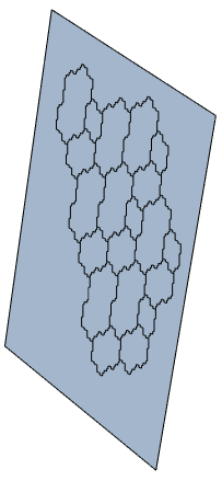
(a) (b)
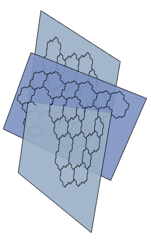
(c)
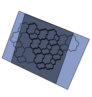
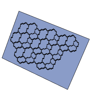
(d) (e)
In Figure 3.16 (a) we show a patch of the collection (for some convenient vector ) of subtiles associated with , while Figure 3.16 (b) shows a patch of the collection associated with the shifted sequence
Note that, since and are not collinear, these patches live in two different planes which is illustrated in Figure 3.16 (c).
In this setting, the set equation in Proposition 3.7.3 says that each element of the collection can be viewed as the union of elements from . In other words, if we take the patch depicted in Figure 3.16 (b) and apply the linear mapping to it, the resulting patch lies in the same plane as the collection and some elements of are unions of elements from . In Figure 3.16 (d) this is illustrated: the image of the patch from Figure 3.16 (b) under the mapping is subdividing some parts of . Figure 3.16 (e) illustrates that, according to Proposition 3.7.6, each element of is a union of elements from .
Note that in Figure 3.16 the collections and are depicted as tilings and the patches of subdivide the elements of without overlap. This is the situation we “dream” of. So far, we only know that elements of are unions of elements of . To realize this ideal situation we need to work more.
3.7.2. An -adic Rauzy fractal is the closure of its interior
The present section is devoted to the interior of the subtiles. We start with a covering result taken from [52, Proposition 6.2]. In its statement we use the following terminology. Let be a collection of subsets of a set . The covering degree of (in ) is the largest number having the property that each is contained in at least elements of .
Lemma 3.7.9.
Let be a sequence of unimodular substitutions and . If is primitive, recurrent, algebraically irreducible, and has finitely balanced language then covers with finite covering degree for each . The covering degree of increases monotonically with .
Proof.
We prove the covering property for . The covering property for as well as the monotonicity of the covering degree follow from this by the set equation in Proposition 3.7.3.
By Proposition 3.7.6 with the choices and we know that
| (3.48) |
holds for each . Because is a locally finite collection of compact sets it suffices to show that is dense in . To prove this we show that the right hand side of (3.48) is dense in for each . To see this note that by the definition of the discrete hyperplane the set of translates in this union satisfies (recall from (3.47) that )
As has rationally independent coordinates by Lemma 3.6.8, the set
is dense in . Since for by primitivity, this yields that
| (3.49) |
is dense in for each . Because was arbitrary and by Lemma 3.7.7 this implies that the right hand side of (3.48) is dense in for each and we are done. ∎
From this result we get the assertion on the interiors of -adic Rauzy fractals.
Proposition 3.7.10.
Let be a sequence of unimodular substitutions over the alphabet and . If is primitive, recurrent, algebraically irreducible, and has finitely balanced language , then is the closure of its interior for each .
Proof.
Choose some . By Lemma 3.7.9 the collection is a locally finite covering of by compact sets for each . Thus by Baire’s theorem for each there is such that . By primitivity of the set equation in Proposition 3.7.3 implies that each contains for some . Thus for each and each we have .
For each and each , Proposition 3.7.3 yields a subdivision of in translates of sets of the form , . The diameters of these sets tend to by Lemma 3.7.7. Since they all contain inner points, the set of inner points of is dense in . In other words, is the closure of its interior. The result now follows by taking . ∎
3.7.3. The generalized left eigenvector
Let be a primitive and recurrent sequence of unimodular substitutions. If we look at the set equation in Proposition 3.7.3 for and we see that it subdivides the sets , , into translates of sets of the form , . In the well-studied substitutive case holds for each , i.e., the sets are subdivided into small copies of themselves. This fact is crucial in most of the proofs of properties of substitutive Rauzy fractals (see e.g. [123]). In our case, in general the sets are not only different for each , but also live in different hyperplanes of .
In what follows we want to deal with this problem by choosing a strictly increasing sequence of integers such that is at least getting closer and closer to in Hausdorff metric when .
To this matter let be a sequence of substitutions that satisfies the assumptions of Theorem 3.7.1. We now successively choose subsequences of the integers to get the desired properties.
- (a)
Consider the set equation in Proposition 3.7.3 for the choices , and , . Look at the subdivision of and . We can hope to get and close to each other in Hausdorff metric if they have the same subdivision structure. From Proposition 3.7.3 we see that these subdivision structures are the same if . Since is recurrent, there exist strictly increasing sequences and such that
(3.50) By recurrence and primitivity it is possible to choose and in a way that there is some such that is the same primitive matrix for all .
- (b)
We know that tends to in Hausdorff metric for by Lemma 3.7.7 so that the subdivision corresponding to the choice , in the set equation gives a subdivision of into sets whose diameter tends to for . However, if we consider , there is no reason for to tend to unless is bounded uniformly in . To this end we need to assume that is -balanced as this implies that is indeed bounded by Proposition 3.6.5. In view of the conditions imposed on in Theorem 3.7.1 it is, however, possible to change the sequence and chosen in (a) in a way that also is -balanced for not depending on .
- (c)
Still (a) and (b) give us no reason for living in a hyperplane close to which is needed in order to get close to in Hausdorff metric. By the compactness of the space of directions in , using the Hilbert metric from Proposition 3.5.5 it is possible to exhibit a vector for which there exists subsequences of and (called and again) such that . Here we set .
Summing up, if the conditions of Theorem 3.7.1 are in force we can choose sequences and satisfying (a), (b), and (c). The vector defined in (c) deserves special attention.
Definition 3.7.11 (Generalized left eigenvector).
A vector as in (c) is called a generalized left eigenvector of .
Sequences and associated with in the above way will just be called associated sequences for in the sequel (they are related to the property PRICE of [52, Definition 5.8]). It turns out that associated sequences are suitable for our purposes. In particular, we get the following result (we refer to [52, Proposition 5.12] for details).
Proposition 3.7.12.
Let be a sequence of substitutions that admits associated sequences and and has a generalized left eigenvector . Then for each
in Hausdorff metric.
Sketch.
By (3.50) in (a) the sets and have the same subdivision structure governed by for . More precisely,
| (3.51) |
By Proposition 3.6.10 the sets tend to in Hausdorff metric for . With more effort, using the balance conditions of (b) and the convergence properties of (c), one can also show that the sets tend to in Hausdorff metric for . So replacing all these sets by on the right hand side of (3.51) changes the sets on the left hand side of (3.51) only very little in Hausdorff metric for large . Thus for large the Hausdorff distance between and is (up to an error tending to for ) bounded by
One can now show that the latter maximum tends to for . Here one uses that by the definition of the generalized left eigenvector in (c) the hyperplanes converge to . ∎
3.7.4. An -adic Rauzy fractal has a boundary of measure zero
We now turn to the boundary of an -adic Rauzy fractal. We start with a result on level subtiles contained in the interior of a given subtile whose detailed proof is contained in [52, Lemma 6.6].
Lemma 3.7.13.
Let be a sequence of unimodular substitutions that satisfies the properties of Theorem 3.7.1 and let associated sequences , , and a generalized left eigenvector be given.
Then there is such that for each there is such that
- (i)
,
- (ii)
for each sufficiently large .
Moreover, the covering degree of does not depend on .
Sketch.
Since the conditions in the lemma imply that (see Proposition 3.7.10) and that the diameter of becomes arbitrarily small for large (see Lemma 3.7.7), assertion (i) follows easily from primitivity.
The fact that and can be chosen in a way that (i) and (ii) hold simultaneously is more difficult to prove. By Proposition 3.7.12 we get that in Hausdorff metric. Moreover, and have the same subdivision structure for steps. This implies that the “inner structure” of these tiles is similar for large . However, as inner points are not respected by the Hausdorff metric, technical difficulties occur and also the “outer structure”, i.e., the structure of the collections and has to be exploited. One can show that if a patch occurs in a discrete hyperplane , then translates of occur relatively densely in each discrete hyperplane provided that is small enough. In particular, containment of translates of a patch is an open property of discrete hyperplanes. Thus, if is large then at level there is a translation such that the sets and have a large patch around the origin in common.
Summing up, this means that the collections converge77 7 In [111] a space of tilings is equipped with a topology by saying that two tilings are close to each other if their tiles are close to each other in Hausdorff metric inside a large ball around the origin. Although and are no tilings, an analogous topology can be used here: and are said to be close to each other if and coincide inside a large ball around the origin and the tiles associated to an element of in each of these two collections are close to each other in Hausdorff metric. to for . This implies that the covering degree of is less than or equal to the covering degree of for large enough. Since the covering degree of is monotonically increasing in by Lemma 3.7.9, the last assertion of the lemma follows.
The fact that the collections converge to and have the same covering degree can now be used to show that inner points of elements of are close to inner points of elements of for large . Using this together with the fact that and have the same subdivision structure for steps, one can show that (i) and (ii) holds simultaneously as claimed. ∎
After these preparations we can also prove the result on the measure of the boundary of -adic Rauzy fractals announced in Theorem 3.7.1.
Proposition 3.7.14.
Let be a sequence of unimodular substitutions over the alphabet that satisfies the assertions of Theorem 3.7.1. Then for each .
Sketch.
Choose and the sequences and as in Lemma 3.7.13 and consider for some (see Figure 3.17 (a)), where is a generalized left eigenvector of . Then subdivide into its level subtiles as shown in Figure 3.17 (b). According to Lemma 3.7.13 (i) there is at least one level subtile which is a subset of ; this is indicated with a black boundary in Figure 3.17 (b). Letting and we therefore gain
Now we subdivide all level subtiles of apart from in level subtiles where is chosen in a way that . This is illustrated in Figure 3.17 (c).


(a) (b)


(c) (d)
We iterate this procedure: each level subtile we got in this way is subdivided in level subtiles. By Lemma 3.7.13 (ii) one of these level subtiles lies in the interior of (see Figure 3.17 (d) for an illustration of this) and, a fortiori, in the interior of If we set
(note that the last equation follows from recurrence of if is chosen large enough) and we obtain
Iterating this further we get for some infinite set that
| (3.52) |
One can show that is uniformly bounded away from . To this end one needs Proposition 3.7.12 and the fact that is chosen in a way that there is some such that is the same primitive matrix for all (see (a) in Section 3.7.3). Now (3.52) yields and, hence, . ∎
3.8. Tilings, coincidence conditions, and combinatorial issues
We now turn to tiling conditions of Rauzy fractals. Already in the substitutive case combinatorial conditions like the strong coincidence condition (see e.g. [18]) or the super coincidence condition and its variants (cf. [36, 51, 91]) have to be imposed in order to gain all the tiling results on Rauzy fractals required for our purposes. Here we discuss an -adic version of these concepts and establish a variety of tiling results. For detailed proofs we refer again to Berthé, Steiner, and Thuswaldner [52]. As before, our aim is to discuss the main ideas and to make these ideas understandable without going into all the technical details.
3.8.1. Multiple tiling and inner subdivision of the subtiles
In this section we prove tiling properties of Rauzy fractals that hold without further combinatorial conditions. Our first result contains a multiple tiling property of the collections of Rauzy fractals defined in (3.35).
Proposition 3.8.1.
Let be a primitive and algebraically irreducible sequence of unimodular substitutions. Assume that there is such that for every there exists such that and the language is -balanced.
If is a generalized left eigenvector of then the collection forms a multiple tiling of the hyperplane .
Sketch.
Let and be associated sequences for . We subdivide the proof in seven observations. In the sequel denotes an open ball in a metric space centered at with radius .
- (i)
Let . As mentioned in the proof of Lemma 3.7.13 one can show that each patch is repetitive in the following sense: there exists and a radius such that for each with and each with a translate of occurs in . This means that each patch occurring in a discrete hyperplane occurs uniformly repetitively in each hyperplane which is close enough to . This general property of discrete hyperplanes is proved in [52, Lemma 6.5].
- (ii)
Let be the covering degree of . Then each point which is covered exactly times by elements of is not contained in the boundary of any element of . Suppose this was wrong and let be the elements containing . Since is a locally finite union of compact sets there is such that doesn’t intersect any . By assumption for some . Thus there is with and, hence, is covered by at most elements of , a contradiction.
- (iii)
Choose which is covered exactly times by elements of . Since the elements of are uniformly bounded, the set of elements of which contain is contained in a set , where is a patch of which is chosen so large that, regardless of how the elements of continue outside , they will not contribute elements of containing because they are bounded and located “too far away” from . Thus, whenever we encounter a translate of in , the point will be covered times by elements of as well. Thus by (i) and (ii) there exist and such that in each ball of radius the hyperplane contains a ball of radius that is covered by exactly elements of .
- (iv)
converges to in a sense described in the proof of Lemma 3.7.13. Thus by (i) the radii and in (iii) can be chosen in a way that in each ball of radius the hyperplane contains a ball of radius that is covered by exactly elements of for large enough.
- (v)
Suppose that is not a multiple tiling. Then there is a set with which is covered at least times. Since the boundaries of the elements of have measure by Proposition 3.7.14, there is , which is covered a least times and which is not contained in the boundary of any element of . Thus there is such that is covered at least times.
- (vi)
Suppose that is not a multiple tiling. By analogous arguments as in (iii), by (v) there exist and such that in each ball of radius the hyperplane contains a ball of radius that is covered by at least elements of .
- (vii)
By Proposition 3.7.6 each element of can be subdivided into elements of . The diameters of the elements of tend to for by Lemma 3.7.7 and the balls of radius occurring in (iv) are shrunk by to ellipsoids contained in balls of radius less than . Thus by (iv) we can chose so large that in each ball of radius in there are points which are covered exactly times by . Thus, by Proposition 3.7.6, in each ball of radius there are points which are covered at most times by . This contradicts (vi) and the result follows.
∎
This result can be generalized to for arbitrary . To establish this generalization one needs to show first that the measures of the subtiles of are determined by
where is the covering degree of the multiple tiling . This can be proved along similar lines as in the substitutive case, see [91, Lemma 2.3]. Using this, measure theoretical considerations lead to the following generalization of Proposition 3.8.1.
Proposition 3.8.2.
Let be a primitive and algebraically irreducible sequence of unimodular substitutions. Assume that there is such that for every there exists such that and the language is -balanced.
Then for each the collection forms a multiple tiling of the hyperplane .
It remains to show that this multiple tiling is actually a tiling. As we will see later, additional assumptions are needed to prove this. However, there is one tiling result which holds without additional assumptions. This result, which concerns the “inner tiling” of by the set equation (3.45) will be proved next.
Proposition 3.8.3.
Let be a primitive and algebraically irreducible sequence of unimodular substitutions. Assume that there is such that for every there exists such that and the language is -balanced.
Proof.
From Proposition 3.8.2 we know that is a multiple tiling for each with multiplicity not depending on . Together with Proposition 3.7.6 this implies that the -th subdivisions of all the tiles in the multiple tiling form a multiple tiling of the same covering degree (for all with ). This is possible only if each tile of is tiled without overlaps by elements of . This proves the result. ∎
3.8.2. Coincidence conditions and tiling properties
Let be a sequence of unimodular substitutions over an alphabet . In view of Example 3.6.2 in order to prove that is measurably conjugate to a rotation on a torus we need two properties of the associated Rauzy fractal . Firstly, the subtiles , , need to be disjoint in measure and secondly, the Rauzy fractal itself has to be a fundamental domain of a (well-chosen) torus. The latter property is equivalent to the fact that admits a lattice tiling of . Setting in Proposition 3.8.2 we obtain that is a multiple tiling of . Since the discrete hyperplane can be written as we see that
Thus is a covering of w.r.t. the lattice and we have to prove that the elements of the union on the right hand side are measure disjoint to get tiling properties of .
We have therefore three types of unions which we want to be disjoint in measure:
- (i)
The unions of subtiles on the right hand side of the set equation (3.45).
- (ii)
The union .
- (iii)
The union .
The elements of the unions in (i) are disjoint in measure by Proposition 3.8.3. One can use this fact in order to prove that the unions in (ii) are disjoint in measure as well. However, to make this proof work we need an additional assumption on .
Definition 3.8.4 (Strong coincidence condition).
A sequence of substitutions over an alphabet satisfies the strong coincidence condition if there is such that for each pair there are and with such that and .
This definition has an easy geometric meaning: it says that the broken lines associated with and have at least one line segment in common for each pair .
Example 3.8.5.
Figure 3.18 shows that the strong coincidence condition is satisfied for the constant sequence with , . Because we are in a case with a two letter alphabet we only have to deal with the instance .
Using the strong coincidence condition we get the following result.
Proposition 3.8.6.
Let be a primitive and algebraically irreducible sequence of unimodular substitutions. Assume that there is such that for every there exists such that and the language is -balanced.
If the strong coincidence condition holds then the subtiles , , are disjoint in measure.
Sketch.
Let and be the associated sequences of . Let and be two subtiles with distinct and assume that the strong coincidence condition holds with . By the definition of the dual in (3.46) this implies that for satisfying there is and a letter such that . Thus the set equation
(see (3.45)) contains and in the union on the right hand side. Proposition 3.8.3 now implies that and are disjoint in measure. Since this is true for arbitrarily large , using results along the line of Proposition 3.7.12 (in particular, [52, Lemma 6.8]) this implies that and are disjoint in measure as well. ∎
What we did in the proof of Proposition 3.8.6 can be explained in a simple way. If the strong coincidence condition holds, each intersection of the subtiles can be realized as an intersection of two elements in the union on the right hand side of the set equation (3.45). Since we know that the elements in the union of the set equation are measure disjoint, the same is true for and . More briefly: in case of strong coincidence the elements in the union in (ii) are special cases of the elements in some union in (i).
The same strategy can be used in order to prove that the unions in (iii) are measure disjoint. To this end we need another type of coincidence condition.
Definition 3.8.7 (Geometric coincidence condition).
A sequence of unimodular substitutions over an alphabet satisfies the geometric coincidence condition if the following is true. For each there is such that for each the set contains a ball of radius of the discrete hyperplane for some .
Along similar lines as Proposition 3.8.6 one can prove the following tiling criterion for Rauzy fractals (see [52, Proposition 7.9]).
Proposition 3.8.8.
Let be a primitive and algebraically irreducible sequence of unimodular substitutions. Assume that there is such that for every there exists such that and the language is -balanced. Then the following assertions are equivalent.
- (i)
The collection forms a tiling of .
- (ii)
The sequence satisfies the geometric coincidence condition.
- (iii)
The sequence satisfies the strong coincidence condition and for each there exists such that contains a ball of radius of for all .
- (iv)
The sequence satisfies the following effective condition: There are , , and , such that
where is chosen in a way that is -balanced.
An (essentially) more restrictive condition than the geometric coincidence condition and its variants in Proposition 3.8.8 is the following one.
Definition 3.8.9 (Geometric finiteness property).
A sequence of unimodular substitutions over an alphabet satisfies the geometric finiteness property if for each there is such that contains the ball for all .
The geometric finiteness property implies that generates a whole discrete plane for , and that is an inner point of the Rauzy fractal (as is proved in [52, Proposition 7.10]). It is immediate that together with the strong coincidence condition the geometric finiteness property is more restrictive than the condition in Proposition 3.8.8 (iii). The name geometric finiteness property comes from the fact that it is related to certain finiteness properties in number representations w.r.t. positional number systems (see for instance Barat et al. [31] for a survey on these objects). By Proposition 3.8.8 (iii) strong coincidence plus geometric finiteness imply that forms a tiling of .
3.8.3. How to check geometric coincidence and geometric finiteness?
In most cases it is easy to check strong coincidence of a sequence of substitutions over an alphabet . For instance, this property trivially holds if starts with the same letter for each . However, it is a priori not so clear how to check geometric coincidence or geometric finiteness and although there is an effective criterion for geometric coincidence contained in Proposition 3.8.8 (iv) this is only suitable for checking single instances. Geometric coincidence asserts that a large piece of a discrete hyperplane can be generated by the dual substitution acting on if is large. If geometric finiteness holds, even a whole discrete hyperplane can be generated by the patches for . The idea of generating discrete hyperplanes in this way using sequences of substitutions coming from generalized continued fraction algorithms goes back to Ito and Ohtsuki [90]. More recently, Berthé et al. [42, 48] provide a systematic study on how to check geometric coincidence as well as geometric finiteness. While [48] concentrates on Arnoux-Rauzy substitutions, the more general treatment in [42] uses substitutions related to the Brun as well as the Jacobi-Perron algorithm as guiding examples. In this section we give a brief discussion of their ideas which are centered around an “annulus property” of stepped hyperplanes generated by .
Let be a sequence of unimodular substitutions over an alphabet and let . The fact that satisfies the geometric coincidence condition in Definition 3.8.7 roughly says that the patch contains a larger and larger ball when is growing. In this section, for the sake of simplicity, we will deal with the geometric finiteness property. Indeed, we will assume that this ball is centered at the origin and instead of we will use as our “seed”. So we want to show that for each there is such that contains the ball for all .
Following [42] we shall reformulate the geometric finiteness property in a more combinatorial way. Let be a patch of a discrete hyperplane containing and interpret its elements as faces as in (3.34). Then the minimal combinatorial radius of is equal to the length of the shortest sequence of faces satisfying , contains a part of the boundary of (regarded as a topological manifold), and for . Intuitively, is the minimal distance between and the boundary of . For instance, one easily checks that the minimal combinatorial radius of the patch on the left hand side of Figure 3.13 is equal to six. Clearly a sequence enjoys the geometric finiteness property if and only if tends to for .
Let . We have to show that the minimal combinatorial radii of the patches tend to for . Since the patches can have complicated shapes there is no obvious way to do this. One approach to prove this property goes back to Ito and Ohtsuki [90] and makes use of “annuli”. Let and suppose that holds for each (this is not a crucial assumption and, if it is not true, can often be gained by blocking the substitutions of the sequence ). Then holds by the definition of (note in particular that for ). The idea is to make sure that whenever is of a certain shape then contains an annulus of positive width. One can then show that if contains the block for times, the patch contains “concentric” annuli and has a minimal combinatorial radius greater than or equal to .
To achieve this we first search for a block such that contains an annulus of positive width, i.e., . If is recurrent, the block occurs infinitely often in . Let with and be an increasing sequence such that . Fix and set and for . Then
| (3.53) |
Because
for (the last step comes from the recurrence property; the case follows along similar lines) each contains some image of under . If the annulus has certain “covering properties” that are described in detail in [42, 48], one can show that images of under are annuli of positive width as well. Thus such an annulus of positive width is contained in each of the pairwise disjoint subsets of and therefore (3.53) implies that the patch contains a “concentric” annulus for each of the (non overlapping) occurrence of the block in . Since an application of maps disjoint annuli to disjoint annuli also with contains such “concentric” annuli. Thus if , the number of such annuli in tends to . Since the above-mentioned covering properties of imply that is simply connected for each and that the same is true for all the patches (see [48]), we gain that the minimal combinatorial radii of the patches tend to for .
The following example shows that this method can be used in order to prove geometric finiteness for large classes of sequences of substitutions.

Example 3.8.10.
We want to illustrate the construction of the annulus around for the case of sequences of Arnoux-Rauzy substitutions (all details for this case can be found in [48]). Suppose that is a recurrent sequence of Arnoux-Rauzy substitutions which contains each of the three Arnoux-Rauzy substitutions (3.18). Then, by recurrence, contains a block in which each Arnoux Rauzy substitution occurs at least twice. In the graph depicted in Figure 3.19 the action of on is illustrated.88 8 We note that in [48] the dual is defined using suffixes of the images of instead of prefixes. Nevertheless, this difference does not change the behavior of significantly and in Figure 3.19 we get the same image as the authors obtained in [48, Figure 1]. The vertices of this graph are patches and there is an edge if . Thus each vertex has an outgoing edge for each (loops and outgoing edges of patches that contain an annulus of positive width around are suppressed). Examining the graph we see that contains an annulus around of positive width whenever the block contains at least two occurrences of each Arnoux-Rauzy substitution. Thus, is a patch which contains together with an annulus of positive width around it.
If one proves that the annulus has the above-mentioned covering properties (which was done in [48]) one can iterate this procedure as indicated above and prove that is simply connected and contains a growing number of “concentric” annuli for growing . Thus the minimal combinatorial radius of tends to for and, hence, has the geometric finiteness property.
Summing up, in Example 3.8.10 we have sketched a proof of the following result.
Proposition 3.8.11.
Let be a sequence of Arnoux-Rauzy substitutions. If is recurrent and contains each of the three Arnoux-Rauzy substitutions then satisfies the geometric finiteness property.
3.9. -adic systems and torus rotations
Let be a sequence of unimodular substitutions over an alphabet with letters. In the past sections we proved a variety of properties of Rauzy fractals. Using all these results makes Rauzy fractals suitable to “see” a rotation on the torus acting on them. This rotation turns out to be measurably conjugate to the underlying -adic system . In this section we prove the according results which form special cases of the main results of [52] and provide some examples.
In Section 3.9.1 we state Theorem 3.9.4, a result that gives the measurable conjugacy between and a torus rotation together with some of its consequences under a set of natural conditions. Section 3.9.2 is devoted to the proof of this result. In Section 3.9.3 we formulate a metric version of Theorem 3.9.4. In particular, for a finite set of substitutions we consider the shift99 9 Note that there are two kinds of shifts: the one just defined acts on the sequence of substitutions , the other one (the -adic shift) acts on the set of sequences which is defined in terms of a single sequence of substitutions . It should cause no confusion that both of these shift mappings are denoted by . acting on all infinite sequences of substitutions taken from . The measure is chosen in a way that this shift becomes ergodic. We prove that the conditions of Theorem 3.9.4 are “generic” w.r.t. the measure if the Pisot condition (3.59) on the Lyapunov exponents associated with a linear cocycle of is in force. Thus under this Pisot condition we gain that -almost all give rise to an -adic system that is measurably conjugate to a torus rotation. This result is the content of Theorem 3.9.5. Section 3.9.4 is devoted to the proof of this result. Finally, Section 3.9.5 gives examples for -adic systems associated with Arnoux-Rauzy and Brun substitutions. This shows that the Pisot condition is satisfied in many natural situations.
3.9.1. Statement of the conjugacy result
Before we state the first main result of this survey we give some terminology. We start with a spectral property of a measurable dynamical system that is “the opposite” of continuous spectrum (see Section 3.3.3; we refer to this section also for the definition of an eigenfunction).
Definition 3.9.1 (Pure discrete spectrum, see [126, Defintion 3.2]).
An ergodic dynamical system on a probability space has pure discrete spectrum if there exists an orthonormal basis of which consists of eigenfunctions of .
It is well known that an ergodic dynamical system on a probability space that has pure discrete spectrum is measurably conjugate to a rotation on a compact abelian group. On the other hand, each ergodic rotation on a compact abelian group has pure discrete spectrum (see for instance [126, Theorems 3.5 and 3.6]; these results can be proved by using character theory and Pontryagin duality for compact abelian groups).
The notion of natural coding came up already in Sections 3.2.4 and 3.3.2 in the framework of Sturmian sequences and Arnoux-Rauzy sequences. Sloppily speaking a natural coding is a coding of a torus rotation that induces translations on the atoms of the partition that was used to define the coding. We give a precise general definition of this concept.
Definition 3.9.2 (Coding and natural coding).
Let be a full-rank lattice in and , a rotation on the torus . Let be a fundamental domain for the lattice and the mapping induced by on . Assume that is a (measure theoretic w.r.t. the Lebesgue measure) partition of .
A sequence is the coding of a point with respect to this partition if holds for each . If, in addition, for each the restriction is given by the translation for some we call a natural coding of .
For the sake of completeness we give the definition of bounded remainder set.
Definition 3.9.3 (Bounded remainder set).
Let be a full-rank lattice in . A subset of is called a bounded remainder set for the rotation , if there exist such that, for a.e. ,
holds for all .
The following result gives sufficient conditions for an -adic system to be measurably conjugate to an irrational rotation on a torus. The subtiles of the Rauzy fractal turn out to be bounded remainder sets for this rotation and induce natural codings of the elements of .
Theorem 3.9.4 (see [52, Theorem 3.1]).
Let be a finite set of unimodular substitutions over a finite alphabet and let be a primitive and algebraically irreducible sequence of substitutions taken from the set . Assume that there is such that for every there exists such that and the language is -balanced.
If the collection forms a tiling of then the following results hold.
- (1)
The -adic shift , with being the unique -invariant Borel probability measure on , is measurably conjugate to a rotation on the torus ; in particular, its measure-theoretic spectrum is purely discrete.
- (2)
Each element of is a natural coding of the torus rotation with respect to the partition of the fundamental domain .
- (3)
The subtile is a bounded remainder set for the torus rotation for each .
3.9.2. Proof of the conjugacy result
In this section we illustrate the proof of Theorem 3.9.4 given in [52]. We assume throughout this section that the sequence satisfies the conditions of Theorem 3.9.4. The main part is the proof of the measurable conjugacy between and a rotation on the torus , where is the cardinality of the underlying alphabet. Here is the unique -invariant Borel probability measure on (see Theorem 3.5.11).
Our first aim is to set up the representation map from to the Rauzy fractal. We define this map using a nested sequence of the subsets
of the Rauzy fractal . In particular, we set
| (3.54) |
To show that is a well-defined continuous surjection one has to prove that the intersection on the right-hand side of (3.54) is a single point. Using the minimality of and the strong convergence property from Proposition 3.6.10 this is done in [52, Section 8].
In the next step one proves that is measurably conjugate to the domain exchange , where is given by
which is illustrated in Figure 3.12. Since is a tiling, the overlaps of the subtiles have measure and, hence, is well defined a.e. w.r.t. the measure on . To prove the asserted conjugacy, we have to show that is bijective -a.e. and that the diagram
| (3.55) |
commutes. Since
| (3.56) |
follows easily by direct calculation it remains to prove the bijectivity assertion. This runs as follows (all statements are true up to measure zero). First observe that satisfies
Therefore, we have and, hence, is a surjective piecewise isometry. Therefore, is bijective. Since the subtiles , , are disjoint in measure and
| (3.57) |
the injectivity of implies that also the elements of the collection of “length subtiles’’1010 10 Not to be confused with the level subtiles introduced in Section 3.7.1. are disjoint in measure. By (3.56) the measure is a shift invariant probability measure on . As by Theorem 3.5.11 there is only one such measure, . Now, essential disjointness of the elements of implies that for all distinct satisfying . As, by (3.57) and Theorem 3.7.1, for all , , the map is -a.e. injective. Since surjectivity follows from the definition of this proves -a.e. bijectivity. Finally, using (3.56), the commutativity of the diagram (3.55) follows from the bijectivity of .
Since forms a tiling of by assumption, the Rauzy fractal is a fundamental domain of the lattice spanned by , . But as holds for each , the canonical projection of onto the torus is equal to the rotation . Thus, if we denote by the canonical projection of to the torus , the diagram
commutes. Note that is to onto, where is the covering degree of , and, hence, a bijection as forms a tiling. This proves the first assertion of Theorem 3.9.4.
3.9.3. A metric result
As mentioned already in Remark 3.7.2 (i), the assumptions of Theorems 3.7.1 and 3.9.4 allow for a metric version of these results. To be more precise, let be a finite set of substitutions and consider the full shift , where is an ergodic -invariant probability measure satisfying some mild conditions. Our aim is to state a version of Theorems 3.5.11, 3.7.1, and 3.9.4 that is valid for -a.e. . This second main result of the present survey is also a special case of a result from Berthé, Steiner, and Thuswaldner [52].
To state our result we need to introduce some new concepts. Let be a finite set of substitutions over the alphabet and consider the shift , where is some -invariant probability measure on . With each we associate the linear cocycle operator (recall that is the incidence matrix of ) and define the Lyapunov exponents of iteratively by
| (3.58) | ||||
for , where denotes the -fold wedge product. We say that satisfies the Pisot condition if
| (3.59) |
(cf. [44, §6.3]). Using these definitions we get the following metric version of Theorems 3.5.11, 3.7.1, and 3.9.4.
Theorem 3.9.5 (see [52, Theorem 3.3]).
Let be a finite set of unimodular substitutions and assume that the shift is ergodic and satisfies the Pisot condition. Assume further that assigns positive measure to every cylinder and that there exists a cylinder corresponding to a substitution with positive incidence matrix. Then, for -almost every the following assertions hold.
- (1)
is minimal and uniquely ergodic (denote the unique -invariant measure by ).
- (2)
Each subtile , , is equal to the closure of its interior and satisfies .
- (3)
If the collection associated with forms a tiling of then is measurably conjugate to a rotation on , each element of is a natural coding of w.r.t. the partition of , and each , , is a bounded remainder set for .
3.9.4. Proof of the metric result
In the present section we give a quite complete proof of Theorem 3.9.5. The idea is to show that each of the conditions posed in Theorem 3.9.4 is generic. A prominent tool in this proof is the Multiplicative Ergodic Theorem (also called Oseledec Theorem; see for instance [8, 3.4.1 Theorem]). Also the famous Poincaré Recurrence Theorem (cf. e.g. [126, Theorem 1.4]), which states that a.e. orbit in a measurable dynamical system starting in a set of positive measure hits infinitely often, will be used. In our setting, the Oseledec theorem has the following consequence.
Proposition 3.9.6.
Let be a finite set of unimodular substitutions over the alphabet and assume that the shift is ergodic with Lyapunov exponents satisfying the Pisot condition (3.59). Assume further that assigns positive measure to every cylinder and that there exists a cylinder corresponding to a substitution with positive incidence matrix. Then for -a.e. the following assertions hold.
- (i)
The sequence is primitive and recurrent, thus the letter frequency vector exists.
- (ii)
For each there exists such that the sequence of incidence matrices satisfies1111 11 Here is the operator norm w.r.t. the Euclidean norm on .
for each .
Proof.
Since puts positive mass on each cylinder, -a.e. is recurrent by Poincaré recurrence. Together with the fact that there is a cylinder corresponding to a positive incidence matrix Poincaré recurrence also implies primitivity for -a.e. . Thus -a.e. has a letter frequency vector by Proposition 3.5.5. This proves (i).
In order to apply the Multiplicative Ergodic Theorem [8, 3.4.1 Theorem] we need to assure log-integrability of the cocycle which, in our case, means that
| (3.60) |
Since finite, the quantity is bounded and therefore (3.60) always holds. Thus, because is a simple Lyapunov exponent, [8, 3.4.1 Theorem] implies that for -a.e. there is a hyperplane such that . This implies that for each there is such that
| (3.61) |
holds for . It remains to show that . However, this follows because for we have that is unbounded because for large the vector is a large vector close to the line . Thus the only hyperplane for which (3.61) can possibly hold is and (ii) follows.
∎
Proposition 3.9.6 is now used in order to show that balance is generic for elements of a shift satisfying the Pisot condition.
Lemma 3.9.7.
Let be a finite set of unimodular substitutions over the alphabet and assume that the shift is ergodic and satisfies the Pisot condition (3.59). Assume further that assigns positive measure to every cylinder and that there exists a cylinder corresponding to a substitution with positive incidence matrix. Then the sets
satisfy
i.e., balance of is a generic property of .
Proof.
By Proposition 3.9.6 we see that for -a.e. the sequence is primitive and recurrent, and for the letter frequency vector (with ) we have
| (3.62) |
We assume that has all these properties and follow the proof of [44, Theorem 5.8]. Let be arbitrary. Since by the proof of Proposition 3.5.3 (iii) each element of has the same language, each factor of is a factor of a limit sequence of and, hence, by (3.4.1) can be written as
| (3.63) |
where and is a prefix and a suffix of for some , respectively, for each and is a factor of for some . To make the notation easier we set and . We mention that (3.63) is the Dumont-Thomas decomposition of which was first introduced in [70]. Using (3.63) and denoting by the standard basis vectors of we have
for each . Since we see that . This can be used to get
Since is a finite set, the quantity is uniformly bounded in . Thus, using (3.62) this implies that is finitely balanced. Since was taken from a set of full measure of this finishes the proof.
∎
Before we can put everything together we need to deal with the genericness of algebraic irreducibility. This has been done in [52, Lemma 8.7] in the following fashion.
Lemma 3.9.8.
Let be a finite set of unimodular substitutions over the alphabet and assume that the shift is ergodic and satisfies the Pisot condition (3.59). If -a.e. sequence is primitive then -a.e. sequence is algebraically irreducible.
Sketch.
Let be a generic sequence with sequence of incidence matrices and fix . Then for the matrix maps the unit sphere into an ellipse whose largest semiaxis tends to infinity and all of whose other semiaxes tend to zero by the Pisot condition. We prove that for large enough there can be only one eigenvalue with .
Indeed, if is large enough then is strictly positive, thus there is a dominant Perron-Frobenius eigenvalue . It corresponds to an eigenvector with strictly positive entries. Suppose that there is another real eigenvalue with and corresponding eigenvector . Since the image of the unit sphere under is an ellipse with the above mentioned properties, the corresponding eigenvector has to have a direction close to for large, because otherwise its length would be shrunk by the application of as can be seen in Figure 3.20.
Thus, if is large enough then must have strictly positive entries. However, such an eigenvector has to belong to the Perron-Frobenius eigenvalue, a contradiction. The case of nonreal eigenvalues can be treated similarly. Thus has only one eigenvalue of modulus greater than or equal to . Since is an unimodular integer matrix, it cannot have as an eigenvalue. This implies that the characteristic polynomial of is irreducible and, hence, is algebraically irreducible. Indeed, we even proved that the characteristic polynomial of is the minimal polynomial of the Pisot number .
∎
We now have all the necessary ingredients to finish the proof of Theorem 3.9.5.
Conclusion of the proof of Theorem 3.9.5.
We show that the conditions of Theorem 3.9.4 are satisfied for -a.e. . To keep things simple we give the proof only for being a Bernoulli measure. Primitivity and algebraic irreducibility hold -a.e. by Proposition 3.9.6 (i) and Lemma 3.9.8, respectively.
It remains to deal with the condition involving recurrence and balance. We claim that there is such that
| (3.64) |
Indeed, since is a Bernoulli measure, is independent from . Thus we have
and the claim (3.64) follows because by assumption and for large enough by Lemma 3.9.7. By another application of Poincaré recurrence (3.64) yields that for -a.e. and for every there is such that and .
Summing up we see that the assumptions of Theorem 3.9.4 are satisfied for -a.e. . Thus Theorem 3.9.5 (1) follows from Theorem 3.5.11, Theorem 3.9.5 (2) follows from Theorem 3.7.1, and Theorem 3.9.5 (3) follows from Theorem 3.9.4.
∎
Remark 3.9.9.
With small amendments in the conclusion of the proof of Theorem 3.9.5 it is possible to prove Theorem 3.9.5 for sofic subshifts of . Even the case of infinitely many substitutions (i.e., ) can be treated provided that the log-integrability condition (3.60) is satisfied. In this case one has to deal with the -adic graph introduced in [44]. As mentioned above, the general result is contained in [52].
3.9.5. Corollaries for Arnoux-Rauzy and Brun systems
We now want to apply the two main theorems to Arnoux-Rauzy as well as Brun -adic systems. Since these systems and their related generalized continued fraction algorithms have been studied quite well in the literature this will yield unconditional results on measurable conjugacy to a torus rotation, natural codings, and bounded remainder sets.
We start with the case of Arnoux-Rauzy systems. Let be the set of Arnoux-Rauzy substitutions defined in (3.18). First we give a version of Theorem 3.9.5 for the -adic sequences taken from .
Corollary 3.9.10 (see [52, Theorem 3.8]).
Let be the set of Arnoux-Rauzy substitutions defined in (3.18) and consider the full shift equipped with an ergodic invariant measure that assigns positive mass to each cylinder. Then -a.e. defines an -adic system that is measurably conjugate to a rotation on the -torus . Moreover, each element of forms a natural coding of w.r.t. the partition defined by the subtiles of the Rauzy fractal . Each of these subtiles is a bounded remainder set of .
Sketch.
It is easy to see that each cylinder containing each of the three substitutions has positive incidence matrix. Thus the result follows from Theorem 3.9.5 if we can establish that satisfies the Pisot condition and that for -a.e. the associated collection of Rauzy fractals forms a tiling. The fact that the Pisot condition holds was proved by Avila and Delecroix [28]. The tiling property is a consequence of Proposition 3.8.8. Indeed, assertion (iii) of this proposition holds by the following results. Firstly, strong coincidence follows from [37, Proposition 4] (or [52, Section 9] where “negative coincidence” was used). The other assertion from Proposition 3.8.8 (iii) is a weaker form of the geometric finiteness property which holds by Proposition 3.8.11 (see also [48, Theorem 4.7]).
∎
With help of the balance properties of Arnoux-Rauzy sequences proved in [43] it is possible to use Theorem 3.9.4 in order to show results for concrete Arnoux-Rauzy systems. For instance it is proved in [52, Corollary 3.9] that any linearly recurrent Arnoux-Rauzy sequence with recurrent directive sequence generates an -adic system that is measurably conjugate to a rotation on a -torus.
For the second class of examples let be the set of Brun substitutions defined in (3.32). In this case a version of Theorem 3.9.5 completely analogous to Corollary 3.9.10 holds.
Corollary 3.9.11 (see [52, Theorem 3.10]).
Let be the set of Brun substitutions defined in (3.32) and consider the full shift equipped with an ergodic invariant measure that assigns positive mass to each cylinder. Then -a.e. defines an -adic system that is measurably conjugate to a rotation on the -torus . Moreover, each element of forms a natural coding of w.r.t. the partition defined by the subtiles of the Rauzy fractal . Each of these subtiles is a bounded remainder set of .
Sketch.
First observe that has positive incidence matrix. One uses again [28] to ensure that the Pisot condition holds (see also [83, 102, 118] for similar results). The tiling property follows from geometric coincidence which is established in [42] for the Brun class.
∎
Contrary to the Arnoux-Rauzy continued fraction algorithm, the Brun algorithm can be performed for all elements with as in (3.24). Thus, using Brun systems we get natural codings for a.a. torus rotations .
3.10. Concluding remarks: Natural extensions, flows, and their Poincaré sections
It remains to extend the ideas and results presented in Section 3.2.5 to generalized continued fraction algorithms and -adic systems on letters. This is the subject of the ongoing paper by Arnoux et al. [12].
It is possible to study natural extensions of generalized continued fraction algorithms (see for instance [19, 21]). In the way we do it in [12], the analogs of the -shaped regions of Section 3.2.5 are “Rauzy-Boxes” which are defined as suspensions of -adic Rauzy fractals. They were introduced in the -adic setting in [52, Section 2.9] but have been studied earlier in the substitutive case, see for instance Ito and Rao [91]. These Rauzy boxes allow nonstationary Markov partitions for so-called “mapping families” in the sense studied by Arnoux and Fisher [15] that can be visualized by restacking -adic Rauzy fractals in a suitable way.
Also Artin’s idea of viewing continued fraction algorithms as Poincaré sections of the geodesic flow on can be generalized. In this generalization the role of the geodesic flow is played by the Weyl Chamber Flow, a diagonal -action on the space of -dimensional lattices. It turns out that each coordinate direction of this -action has a Poincaré section which is arithmetically coded by a generalized continued fraction algorithm. Geometrically, this is visualized by deforming a given Rauzy box (one for each coordinate) by the action of the Weyl Chamber Flow and restacking it accordingly as soon as a Poincaré section is reached.
Details of all this will be contained in [12].
3.11. Acknowledgements
I warmly thank Shigeki Akiyama and Pierre Arnoux for inviting me to contribute to this volume. I very much appreciate their constant encouragement and support, and the many discussions I had with them. Moreover, I am indebted to Valérie Berthé, Sébastien Labbé, and Wolfgang Steiner for their suggestions.
References
- [1] Adamczewski, B.: Balances for fixed points of primitive substitutions. Theoret. Comput. Sci. 307(1), 47–75 (2003). Words
- [2] Akiyama, S.: Self affine tilings and Pisot numeration systems. In: K. Győry, S. Kanemitsu (eds.) Number Theory and its Applications, pp. 1–17. Kluwer (1999)
- [3] Akiyama, S.: On the boundary of self affine tilings generated by Pisot numbers. J. Math. Soc. Japan 54(2), 283–308 (2002)
- [4] Akiyama, S., Barge, M., Berthé, V., Lee, J.Y., Siegel, A.: On the Pisot substitution conjecture. In: Mathematics of aperiodic order, Progr. Math., vol. 309, pp. 33–72. Birkhäuser/Springer, Basel (2015)
- [5] Akiyama, S., Sadahiro, T.: A self-similar tiling generated by the minimal Pisot number. In: Proceedings of the 13th Czech and Slovak International Conference on Number Theory (Ostravice, 1997), vol. 6, pp. 9–26 (1998)
- [6] Allouche, J.P., Shallit, J.: Automatic sequences. Cambridge University Press, Cambridge (2003). Theory, applications, generalizations
- [7] Andres, A., Acharya, R., Sibata, C.: Discrete analytical hyperplanes. Graphical Models and Image Processing 59, 302–309 (1997)
- [8] Arnold, L.: Random dynamical systems. Springer Monographs in Mathematics. Springer-Verlag, Berlin (1998)
- [9] Arnoux, P.: Un exemple de semi-conjugaison entre un échange d’intervalles et une translation sur le tore. Bull. Soc. Math. France 116(4), 489–500 (1989) (1988)
- [10] Arnoux, P.: Le codage du flot géodésique sur la surface modulaire. Enseign. Math. (2) 40(1-2), 29–48 (1994)
- [11] Arnoux, P.: Continued fractions: natural extensions and invariant measures. In: Natural extension of arithmetic algorithms and S-adic system, RIMS Kôkyûroku Bessatsu, B58, pp. 19–32. Res. Inst. Math. Sci. (RIMS), Kyoto (2016)
- [12] Arnoux, P., Berthé, V., Minervino, M., Steiner, W., Thuswaldner, J.: Nonstationary Markov partitions, flows on homogeneous spaces, and continued fractions (2018). In preparation
- [13] Arnoux, P., Ferenczi, S., Hubert, P.: Trajectories of rotations. Acta Arith. 87(3), 209–217 (1999)
- [14] Arnoux, P., Fisher, A.M.: The scenery flow for geometric structures on the torus: the linear setting. Chinese Ann. Math. Ser. B 22(4), 427–470 (2001)
- [15] Arnoux, P., Fisher, A.M.: Anosov families, renormalization and non-stationary subshifts. Ergodic Theory Dynam. Systems 25(3), 661–709 (2005)
- [16] Arnoux, P., Furukado, M., Harriss, E., Ito, S.: Algebraic numbers, free group automorphisms and substitutions on the plane. Trans. Amer. Math. Soc. 363(9), 4651–4699 (2011)
- [17] Arnoux, P., Harriss, E.: What is … a Rauzy fractal? Notices Amer. Math. Soc. 61(7), 768–770 (2014)
- [18] Arnoux, P., Ito, S.: Pisot substitutions and Rauzy fractals. Bull. Belg. Math. Soc. Simon Stevin 8(2), 181–207 (2001). Journées Montoises d’Informatique Théorique (Marne-la-Vallée, 2000)
- [19] Arnoux, P., Labbé, S.: On some symmetric multidimensional continued fraction algorithms. Ergodic Theory and Dynamical Systems 38(5), 1601–1626 (2018)
- [20] Arnoux, P., Mizutani, M., Sellami, T.: Random product of substitutions with the same incidence matrix. Theoret. Comput. Sci. 543, 68–78 (2014)
- [21] Arnoux, P., Nogueira, A.: Mesures de Gauss pour des algorithmes de fractions continues multidimensionnelles. Ann. Sci. École Norm. Sup. (4) 26(6), 645–664 (1993)
- [22] Arnoux, P., Rauzy, G.: Représentation géométrique de suites de complexité . Bull. Soc. Math. France 119(2), 199–215 (1991)
- [23] Arnoux, P., Schmidt, T.A.: Cross sections for geodesic flows and -continued fractions. Nonlinearity 26(3), 711–726 (2013)
- [24] Arnoux, P., Schmidt, T.A.: Commensurable continued fractions. Discrete Contin. Dyn. Syst. 34(11), 4389–4418 (2014)
- [25] Arnoux, P., Starosta, Š.: The Rauzy gasket. In: Further developments in fractals and related fields, Trends Math., pp. 1–23. Birkhäuser/Springer, New York (2013)
- [26] Artin, E.: Ein mechanisches System mit quasiergodischen Bahnen. Abh. Math. Sem. Univ. Hamburg 3(1), 170–175 (1924)
- [27] Auslander, J.: Minimal flows and their extensions, North-Holland Mathematics Studies, vol. 153. North-Holland Publishing Co., Amsterdam (1988). Notas de Matemática [Mathematical Notes], 122
- [28] Avila, A., Delecroix, V.: Some monoids of Pisot matrices (2015). Preprint, http://arxiv.org/abs/1506.03692
- [29] Avila, A., Hubert, P., Skripchenko, A.: Diffusion for chaotic plane sections of 3-periodic surfaces. Invent. Math. 206(1), 109–146 (2016)
- [30] Avila, A., Hubert, P., Skripchenko, A.: On the Hausdorff dimension of the Rauzy gasket. Bull. Soc. Math. France 144(3), 539–568 (2016)
- [31] Barat, G., Berthé, V., Liardet, P., Thuswaldner, J.: Dynamical directions in numeration. Ann. Inst. Fourier (Grenoble) 56(7), 1987–2092 (2006). Numération, pavages, substitutions
- [32] Barge, M.: Pure discrete spectrum for a class of one-dimensional substitution tiling systems. Discrete Contin. Dyn. Syst. 36(3), 1159–1173 (2016)
- [33] Barge, M.: The Pisot conjecture for -substitutions. Ergodic Theory Dynam. Systems 38(2), 444–472 (2018)
- [34] Barge, M., Diamond, B.: Coincidence for substitutions of Pisot type. Bull. Soc. Math. France 130(4), 619–626 (2002)
- [35] Barge, M., Kellendonk, J.: Proximality and pure point spectrum for tiling dynamical systems. Michigan Math. J. 62(4), 793–822 (2013)
- [36] Barge, M., Kwapisz, J.: Geometric theory of unimodular Pisot substitutions. Amer. J. Math. 128(5), 1219–1282 (2006)
- [37] Barge, M., Štimac, S., Williams, R.F.: Pure discrete spectrum in substitution tiling spaces. Discrete Contin. Dyn. Syst. 33(2), 579–597 (2013)
- [38] Belov, A.Y., Kondakov, G.V., Mitrofanov, I.V.: Inverse problems of symbolic dynamics. In: Algebraic methods in dynamical systems, Banach Center Publ., vol. 94, pp. 43–60. Polish Acad. Sci. Inst. Math., Warsaw (2011)
- [39] Bernoulli, J.: Sur une nouvelle espece de calcul. Recueil pour les Astronomes, Berlin 1, 255–284 (1772)
- [40] Berstel, J.: Transductions and context-free languages, Leitfäden der Angewandten Mathematik und Mechanik [Guides to Applied Mathematics and Mechanics], vol. 38. B. G. Teubner, Stuttgart (1979)
- [41] Berthé, V.: Multidimensional Euclidean algorithms, numeration and substitutions. Integers 11B, A2 (2011)
- [42] Berthé, V., Bourdon, J., Jolivet, T., Siegel, A.: A combinatorial approach to products of Pisot substitutions. Ergodic Theory Dynam. Systems 36(6), 1757–1794 (2016)
- [43] Berthé, V., Cassaigne, J., Steiner, W.: Balance properties of Arnoux-Rauzy words. Internat. J. Algebra Comput. 23(4), 689–703 (2013)
- [44] Berthé, V., Delecroix, V.: Beyond substitutive dynamical systems: -adic expansions. RIMS lecture note ‘Kôkyûroku Bessatsu’ B46, 81–123 (2014)
- [45] Berthé, V., Domenjoud, E., Jamet, D., Provençal, X.: Fully subtractive algorithm, tribonacci numeration and connectedness of discrete planes. In: Numeration and substitution 2012, RIMS Kôkyûroku Bessatsu, B46, pp. 159–174. Res. Inst. Math. Sci. (RIMS), Kyoto (2014)
- [46] Berthé, V., Ferenczi, S., Zamboni, L.Q.: Interactions between dynamics, arithmetics and combinatorics: the good, the bad, and the ugly. In: Algebraic and topological dynamics, Contemp. Math., vol. 385, pp. 333–364. Amer. Math. Soc., Providence, RI (2005)
- [47] Berthé, V., Holton, C., Zamboni, L.Q.: Initial powers of Sturmian sequences. Acta Arith. 122(4), 315–347 (2006)
- [48] Berthé, V., Jolivet, T., Siegel, A.: Substitutive Arnoux-Rauzy sequences have pure discrete spectrum. Unif. Distrib. Theory 7(1), 173–197 (2012)
- [49] Berthé, V., Labbé, S.: Factor complexity of -adic words generated by the Arnoux-Rauzy-Poincaré algorithm. Adv. in Appl. Math. 63, 90–130 (2015)
- [50] Berthé, V., Minervino, M., Steiner, W., Thuswaldner, J.: The -adic Pisot conjecture on two letters. Topology Appl. 205, 47–57 (2016)
- [51] Berthé, V., Siegel, A., Thuswaldner, J.M.: Substitutions, Rauzy fractals, and tilings. In: Combinatorics, Automata and Number Theory, Encyclopedia of Mathematics and its Applications, vol. 135. Cambridge University Press (2010)
- [52] Berthé, V., Steiner, W., Thuswaldner, J.M.: Geometry, dynamics, and arithmetic of -adic shifts. Ann. Inst. Fourier (Grenoble) 69(3), 1347–1409 (2019)
- [53] Bezuglyi, S., Kwiatkowski, J., Medynets, K., Solomyak, B.: Invariant measures on stationary Bratteli diagrams. Ergodic Theory Dynam. Systems 30(4), 973–1007 (2010)
- [54] Bezuglyi, S., Kwiatkowski, J., Medynets, K., Solomyak, B.: Finite rank Bratteli diagrams: structure of invariant measures. Trans. Amer. Math. Soc. 365(5), 2637–2679 (2013)
- [55] Birkhoff, G.: Extensions of Jentzsch’s theorem. Trans. Amer. Math. Soc. 85, 219–227 (1957)
- [56] Boshernitzan, M.: A unique ergodicity of minimal symbolic flows with linear block growth. J. Analyse Math. 44, 77–96 (1984/85)
- [57] Boyland, P., Severa, W.: Geometric representation of the infimax S-adic family. Fund. Math. 240(1), 15–50 (2018)
- [58] Brentjes, A.J.: Multidimensional continued fraction algorithms, Mathematical Centre Tracts, vol. 145. Mathematisch Centrum, Amsterdam (1981)
- [59] Brun, V.: Algorithmes euclidiens pour trois et quatre nombres. In: Treizième congrès des mathèmaticiens scandinaves, tenu à Helsinki 18-23 août 1957, pp. 45–64. Mercators Tryckeri, Helsinki (1958)
- [60] Burger, E.B., Gell-Redman, J., Kravitz, R., Walton, D., Yates, N.: Shrinking the period lengths of continued fractions while still capturing convergents. J. Number Theory 128(1), 144–153 (2008)
- [61] Canterini, V., Siegel, A.: Geometric representation of substitutions of Pisot type. Trans. Amer. Math. Soc. 353(12), 5121–5144 (2001)
- [62] Cassaigne, J., Ferenczi, S., Messaoudi, A.: Weak mixing and eigenvalues for Arnoux-Rauzy sequences. Ann. Inst. Fourier (Grenoble) 58(6), 1983–2005 (2008)
- [63] Cassaigne, J., Ferenczi, S., Zamboni, L.Q.: Imbalances in Arnoux-Rauzy sequences. Ann. Inst. Fourier (Grenoble) 50(4), 1265–1276 (2000)
- [64] Cassaigne, J., Labbé, S., Leroy, J.: A set of sequences of complexity . In: Combinatorics on words, Lecture Notes in Comput. Sci., vol. 10432, pp. 144–156. Springer, Cham (2017)
- [65] Cassaigne, J., Nicolas, F.: Factor complexity. In: Combinatorics, automata and number theory, Encyclopedia Math. Appl., vol. 135, pp. 163–247. Cambridge Univ. Press, Cambridge (2010)
- [66] Cortez, M.I., Durand, F., Host, B., Maass, A.: Continuous and measurable eigenfunctions of linearly recurrent dynamical Cantor systems. J. London Math. Soc. (2) 67(3), 790–804 (2003)
- [67] Coven, E.M., Hedlund, G.A.: Sequences with minimal block growth. Math. Systems Theory 7, 138–153 (1973)
- [68] Delecroix, V., Hejda, T., Steiner, W.: Balancedness of Arnoux-Rauzy and Brun words. In: WORDS, Lecture Notes in Computer Science, vol. 8079, pp. 119–131. Springer (2013)
- [69] DeLeo, R., Dynnikov, I.A.: Geometry of plane sections of the infinite regular skew polyhedron . Geom. Dedicata 138, 51–67 (2009)
- [70] Dumont, J.M., Thomas, A.: Systemes de numeration et fonctions fractales relatifs aux substitutions. Theoret. Comput. Sci. 65(2), 153–169 (1989)
- [71] Durand, F.: Linearly recurrent subshifts have a finite number of non-periodic subshift factors. Ergodic Theory Dynam. Systems 20, 1061–1078 (2000)
- [72] Durand, F.: Corrigendum and addendum to: “Linearly recurrent subshifts have a finite number of non-periodic subshift factors” [Ergodic Theory Dynam. Systems 20 (2000), no. 4, 1061–1078]. Ergodic Theory Dynam. Systems 23, 663–669 (2003)
- [73] Durand, F., Leroy, J., Richomme, G.: Do the properties of an -adic representation determine factor complexity? J. Integer Seq. 16(2), Article 13.2.6, 30 pp. (2013)
- [74] Ei, H.: Some properties of invertible substitutions of rank , and higher dimensional substitutions. Osaka J. Math. 40(2), 543–562 (2003)
- [75] Ei, H., Ito, S., Rao, H.: Atomic surfaces, tilings and coincidences. II. Reducible case. Ann. Inst. Fourier (Grenoble) 56(7), 2285–2313 (2006). Numération, pavages, substitutions
- [76] Einsiedler, M., Ward, T.: Ergodic theory with a view towards number theory, Graduate Texts in Mathematics, vol. 259. Springer-Verlag London, Ltd., London (2011)
- [77] Ferenczi, S.: Rank and symbolic complexity. Ergodic Theory Dynam. Systems 16(4), 663–682 (1996)
- [78] Ferenczi, S., Fisher, A.M., Talet, M.: Minimality and unique ergodicity for adic transformations. J. Anal. Math. 109, 1–31 (2009)
- [79] Fernique, T.: Multidimensional Sturmian sequences and generalized substitutions. Internat. J. Found. Comput. Sci. 17(3), 575–599 (2006)
- [80] Fernique, T.: Generation and recognition of digital planes using multi-dimensional continued fractions. In: Discrete geometry for computer imagery, Lecture Notes in Comput. Sci., vol. 4992, pp. 33–44. Springer, Berlin (2008)
- [81] Fisher, A.M.: Nonstationary mixing and the unique ergodicity of adic transformations. Stoch. Dyn. 9(3), 335–391 (2009)
- [82] Fogg, N.P.: Substitutions in dynamics, arithmetics and combinatorics, Lecture Notes in Mathematics, vol. 1794. Springer-Verlag, Berlin (2002)
- [83] Fujita, T., Ito, S., Keane, M., Ohtsuki, M.: On almost everywhere exponential convergence of the modified Jacobi-Perron algorithm: a corrected proof. Ergodic Theory Dynam. Systems 16(6), 1345–1352 (1996)
- [84] Furstenberg, H.: Stationary processes and prediction theory. Annals of Mathematics Studies, No. 44. Princeton University Press, Princeton, N.J. (1960)
- [85] Halmos, P.R.: Lectures on ergodic theory. Chelsea Publishing Co., New York (1960)
- [86] Holton, C., Zamboni, L.Q.: Geometric realizations of substitutions. Bull. Soc. Math. France 126(2), 149–179 (1998)
- [87] Hopcroft, J.E., Ullman, J.D.: Introduction to automata theory, languages, and computation. Addison-Wesley Publishing Co., Reading, Mass. (1979). Addison-Wesley Series in Computer Science
- [88] Hubert, P., Messaoudi, A.: Best simultaneous Diophantine approximations of Pisot numbers and Rauzy fractals. Acta Arith. 124(1), 1–15 (2006)
- [89] Ito, S., Kimura, M.: On Rauzy fractal. Japan J. Indust. Appl. Math. 8(3), 461–486 (1991)
- [90] Ito, S., Ohtsuki, M.: Parallelogram tilings and Jacobi-Perron algorithm. Tokyo J. Math. 17(1), 33–58 (1994)
- [91] Ito, S., Rao, H.: Atomic surfaces, tilings and coincidence. I. Irreducible case. Israel J. Math. 153, 129–155 (2006)
- [92] Jamet, D., Lafrenière, N., Provençal, X.: Generation of digital planes using generalized continued-fractions algorithms. In: Discrete geometry for computer imagery, Lecture Notes in Comput. Sci., vol. 9647, pp. 45–56. Springer, [Cham] (2016)
- [93] Jamet, D., Toutant, J.L.: On the connectedness of rational arithmetic discrete hyperplanes. In: Discrete geometry for computer imagery, Lecture Notes in Comput. Sci., vol. 4245, pp. 223–234. Springer, Berlin (2006)
- [94] Katok, A.: Interval exchange transformations and some special flows are not mixing. Israel J. Math. 35(4), 301–310 (1980)
- [95] Labbé, S.: 3-dimensional continued fraction algorithms cheat sheets (2015). http://arxiv.org/abs/1511.08399
- [96] Lagarias, J., Wang, Y.: Self-affine tiles in . Adv. Math. 121, 21–49 (1996)
- [97] Leroy, J.: Some improvements of the -adic conjecture. Adv. in Appl. Math. 48(1), 79–98 (2012)
- [98] Leroy, J.: An -adic characterization of minimal subshifts with first difference of complexity . Discrete Math. Theor. Comput. Sci. 16(1), 233–286 (2014)
- [99] Levitt, G.: La dynamique des pseudogroupes de rotations. Invent. Math. 113(3), 633–670 (1993)
- [100] Loridant, B., Minervino, M.: Geometrical models for a class of reducible Pisot substitutions. Discrete Comput. Geom. 60, 981–1028 (2018)
- [101] Lothaire, M.: Algebraic combinatorics on words, Encyclopedia of Mathematics and its Applications, vol. 90. Cambridge University Press, Cambridge (2002). A collective work by J. Berstel, D. Perrin, P. Seebold, J. Cassaigne, A. De Luca, S. Varricchio, A. Lascoux, B. Leclerc, J.-Y. Thibon, V. Bruyere, C. Frougny, F. Mignosi, A. Restivo, C. Reutenauer, D. Foata, G.-N. Han, J. Desarmenien, V. Diekert, T. Harju, J. Karhumaki and W. Plandowski, with a preface by J. Berstel and D. Perrin
- [102] Meester, R.: A simple proof of the exponential convergence of the modified Jacobi-Perron algorithm. Ergodic Theory Dynam. Systems 19(4), 1077–1083 (1999)
- [103] Messaoudi, A.: Frontière du fractal de Rauzy et système de numération complexe. Acta Arith. 95(3), 195–224 (2000)
- [104] Messaoudi, A.: Propriétés arithmétiques et topologiques d’une classe d’ensembles fractales. Acta Arith. 121(4), 341–366 (2006)
- [105] Minervino, M., Steiner, W.: Tilings for Pisot beta numeration. Indag. Math. (N.S.) 25(4), 745–773 (2014)
- [106] Minervino, M., Thuswaldner, J.M.: The geometry of non-unit Pisot substitutions. Ann. Inst. Fourier (Grenoble) 64(4), 1373–1417 (2014)
- [107] Morse, M., Hedlund, G.A.: Symbolic dynamics II. Sturmian trajectories. Amer. J. Math. 62, 1–42 (1940)
- [108] Nakada, H., Ito, S., Tanaka, S.: On the invariant measure for the transformations associated with some real continued-fractions. Keio Engrg. Rep. 30(13), 159–175 (1977)
- [109] Perron, O.: Grundlagen für eine Theorie des Jacobischen Kettenbruchalgorithmus. Math. Ann. 64(1), 1–76 (1907)
- [110] Queffélec, M.: Substitution dynamical systems—spectral analysis, Lecture Notes in Mathematics, vol. 1294, second edn. Springer-Verlag, Berlin (2010)
- [111] Radin, C., Wolff, M.: Space tilings and local isomorphism. Geom. Dedicata 42(3), 355–360 (1992)
- [112] Rauzy, G.: Une généralisation du développement en fraction continue. In: Séminaire Delange-Pisot-Poitou, 18e année: 1976/77, Théorie des nombres, Fasc. 1, pp. Exp. No. 15, 16. Secrétariat Math., Paris (1977)
- [113] Rauzy, G.: échanges d’intervalles et transformations induites. Acta Arith. 34(4), 315–328 (1979)
- [114] Rauzy, G.: Nombres algébriques et substitutions. Bull. Soc. Math. France 110(2), 147–178 (1982)
- [115] Reveillès, J.P.: Géométrie discrète, calculs en nombres entiers et algorithmes. Ph.D. thesis, Université Louis Pasteur, Strasbourg (1991)
- [116] Rohlin, V.A.: Exact endomorphism of a Lebesgue space. Magyar Tud. Akad. Mat. Fiz. Oszt. Közl. 14, 443–474 (1964)
- [117] Sano, Y., Arnoux, P., Ito, S.: Higher dimensional extensions of substitutions and their dual maps. J. Anal. Math. 83, 183–206 (2001)
- [118] Schratzberger, B.R.: The exponent of convergence for Brun’s algorithm in two dimensions. Österreich. Akad. Wiss. Math.-Natur. Kl. Sitzungsber. II 207, 229–238 (1999) (1998)
- [119] Schweiger, F.: Multidimensional continued fractions. Oxford Science Publications. Oxford University Press, Oxford (2000)
- [120] Selmer, E.S.: Continued fractions in several dimensions. Nordisk Nat. Tidskr. 9, 37–43, 95 (1961)
- [121] Series, C.: The modular surface and continued fractions. J. London Math. Soc. (2) 31(1), 69–80 (1985)
- [122] Siegel, A.: Représentation des systèmes dynamiques substitutifs non unimodulaires. Ergodic Theory Dynam. Systems 23(4), 1247–1273 (2003)
- [123] Siegel, A., Thuswaldner, J.M.: Topological properties of Rauzy fractals. Mém. Soc. Math. Fr. (N.S.) 118, 144pp (2009)
- [124] Sirvent, V.F., Wang, Y.: Self-affine tiling via substitution dynamical systems and Rauzy fractals. Pacific J. Math. 206(2), 465–485 (2002)
- [125] Viana, M.: Ergodic theory of interval exchange maps. Rev. Mat. Complut. 19(1), 7–100 (2006)
- [126] Walters, P.: An introduction to ergodic theory, Graduate Texts in Mathematics, vol. 79. Springer-Verlag, New York (1982)