Spin geometric-phases in hopping magnetoconductance
Abstract
We identify theoretically the geometric phases of the electrons’ spinor that can be detected in measurements of charge and spin transport through Aharonov-Bohm interferometers threaded by a magnetic flux (in units of the flux quantum) where Rashba spin-orbit and Zeeman interactions are active. We show that the combined effect of these two interactions produces a [in addition to the usual ] dependence of the magnetoconductance, whose amplitude is proportional to the Zeeman field. Therefore, although the magnetoconductance is an even function of the magnetic field, it is not a periodic function of it, and the widely-used concept of a phase shift in the Aharonov-Bohm oscillations, as indicated in previous work, is not applicable. We find the directions of the spin-polarizations in the system, and show that in general (even without the Zeeman term) the spin currents are not conserved, implying the generation of magnetization in the terminals attached to the interferometer.
I Introduction
The phase factor induced on the spin wave-functions of electrons moving in an electric field is generally attributed to the Aharonov-Casher effect, AC the electromagnetic dual of the Aharonov-Bohm effect. AB The physical origin of this phenomenon is the spin-orbit interaction, that gives rise to a momentum-dependent magnetic field perpendicular to both the propagation direction of the electron waves and the electric field which creates it. Attempts to monitor the Aharonov-Casher phase factor utilize various designs of spin interferometers in low-dimensional electronic structures. Of particular significance in this context is the spin-orbit interaction generated by the Bychkov-Rashba mechanism, Bychkov which can be controlled via asymmetric gate electrodes. Takayanagi Indeed, measuring the resistance of an array of mesoscopic semiconductor rings placed in an asymmetric quantum well whose asymmetry was tuned by a gate voltage, enabled the demonstration of the Aharonov-Casher interference. Bergsten The value of the spin-orbit interaction parameter which was deduced from the interference patterns was in agreement with the one derived from Shubnikov-de Haas analyses (measured in the presence of orbital magnetic fields).
The Aharonov-Casher phase comprises two contributions. Qian Besides the standard, “dynamic phase", related to the precession of the spins around a constant magnetic-field direction, there appears also a geometric (topological) phase: the Berry phase. Berry; Vanderbilt It is accumulated when the direction of the spin-orbit-induced magnetic field follows adiabatically a closed trajectory in space and is proportional to the solid angle subtended by the direction of that field. Under non-adiabatic conditions the spin precession axis is no longer parallel to the spin-orbit-induced magnetic field. Then the acquired phse is termed the Aharonov-Anandan phase Anandan (which generalizes the Berry phase).
The geometric phase on the spin wave-function and the way it affects physical observables have been the subject of intense theoretical and experimental research in recent years. This phase was predicted to lead to topological persistent spin-currents in closed loops even in the absence of electromagnetic fluxes Loss; Oh or in rings coupled spin-symmetrically to external reservoirs. Ellner As the Aharonov-Casher phase modifies the transmission of electrons through multiply-connected mesoscopic structures, Avishai it is natural to explore its effects on Aharonov-Bohm oscillations measured on such devices. In the absence of the spin-orbit interaction, and neglecting the Zeeman field on the spin magnetic moment, the magnetoconductance of Aharonov-Bohm interferometers is periodic in the magnetic flux (measured in units of the flux quantum) which is due to an external magnetic field normal to the plane of the interferometer. It was shown Meir that the spin-orbit interaction modifies the magnetic-flux dependence of the spectrum of electrons in a one-dimensional ring into a dependence for the two relevant spin directions. Here, is the Aharonov-Casher phase that results from the spin-orbit interaction. A spin-interference device, in which the phase difference between the spin wave-functions traveling in the clockwise and anti-clockwise directions can be measured, was indeed proposed. Nitta The idea was elaborated upon theoretically, Peeters; Frustaglia; Capozza and measurements were carried out in a GaAs two-dimensional hole system with a strong spin-orbit coupling, Yau and in ring structures fabricated from HgTe/HgCdTe quantum wells. Konig The Aharonov-Casher phase was also detected in measurements of interference patterns of the magnetoconductance of electrons traveling coherently in opposite directions around arrays of InAlAs/InGaAs mesoscopic semiconductor rings. Nagasawa
While Aharonov-Bohm conductance oscillations allow for the experimental detection of the Aharonov-Casher phase, attempts to separate the dynamic and topological aspects of this phase rely on additional information, extracted either from simulations Yau or from comparisons with theoretical expressions Qian; Frustaglia which express the geometric and dynamic phases in terms of the Aharonov-Casher phase calculated for a circular ring. For such rings, the Aharonov-Casher phase indeed determines both the dynamic and the geometric Aharonov-Anandan phases. In contrast, we find that for general configurations there exist no such simple relations, and it may not be possible to extract the dynamic and geometric phases from the Aharonov-Bohm interference patterns.
This paper is aimed to identify the geometric phases of the electrons’ spinor that can be detected in measurements of charge and spin transport through Aharonov-Bohm interferometers in which both the Rashba spin-orbit and Zeeman interactions are active (the latter is due to a magnetic field normal to the plane of the interferometer). In particular, we consider the possible appearance of a phase shift in the (periodic) dependence of the magnetoconductance on the Aharonov-Bohm flux , and the phases which determine the directions of the spin magnetizations in the two reservoirs connected to the interferometer. The phase shift of is especially intriguing: perhaps the first to propose that the spin-orbit and Zeeman interactions join together to shift the Aharonov-Bohm oscillations for each spin direction by the Berry phase were Aronov and Lyanda-Geller. Lyanda Operating within the adiabatic limit where both interaction energies are much larger than the angular kinetic energy, they predicted phase shifts in the Aharonov-Bohm oscillations of the transmission of each spin direction. Aronov and Lyanda-Geller related these phase shifts to the Berry phase that depends on the Zeeman energy. A similar conclusion appears in Ref. Peeters, where this deviation is attributed to the Aharonov-Casher phase. Reference Lyanda has been criticised in the literature, because it used a non-hermitian Hamiltonian, Morpurgo and because it was claimed Yi that it had not accounted properly for the effects of the time-reversal symmetry breaking by the Zeeman field. We do not share this second argument: our results below, though obtained in an entirely different regime, indicate that Grosso Modo the transmission given in Ref. Lyanda has the correct form, namely, the (longitudinal) conductance is an even function of the magnetic field, as required by the Onsager relations, though it is not periodic in it. However, we find that in general the deviation away from periodicity is not related to the Berry phase.
In contrast to the theoretical works surveyed above, which adopt a continuous description for the Hamiltonian of the electrons on a circular ring (with the exception of Ref. Avishai), we consider transport in the hopping regime. In other words, the kinetic energy of the electrons when on the interferometer loop is modelled in a tight-binding picture. This necessitates the detailed knowledge of the tunneling matrix elements between localized states when the tunneling electrons are subjected to spin-orbit interactions and Zeeman and orbital magnetic fields, which we derive in Appendix B. Calculating the charge (particle) current through an arbitrarily-shaped single-channel triangular interferometer coupled to two non-polarized electronic reservoirs, we find that quite generally, the interference-related part of the electrical conductance in the absence of the Zeeman interaction is proportional to , as indeed has been predicted. Avishai; Meir When the Zeeman interaction is included the pattern of the Aharonov-Bohm oscillations is modified: there appears a term in the interference-induced transmission, whose amplitude is proportional to the Zeeman field and which vanishes without the spin-orbit interaction. The coefficient of this term depends on details of the triangular structure. Although this field-dependent amplitude breaks the periodicity of the conductance in the magnetic field, thus eliminating the concept of a phase shift, the entire conductance still obeys the Onsager relations. In this respect we agree with the final result of Ref. Lyanda. However, there is no obvious relation between this amplitude and the angles that determine the spin-magnetization directions. Therefore, as opposed to the finding of Ref. Lyanda, in general measuring the interference pattern of Aharonov-Bohm oscillations yields no information on the Berry phase. As Qian and Su Qian show, the limit of a regular polygon with edges approaches the perfect circle, and it is possible that for that geometry one recovers the Aronov-Lyanda-Geller Lyanda predictions. However, we do not get such results even for an equilateral triangle, and therefore we suspect that the circle is very special, and it is not possible to deduce the Berry phase from transport measurements on a general interferometer.
The Berry phase is usually associated with the direction of the electron’s spin polarization once it tunnels around the closed loop. It turns out that for a circular loop the spin-orbit interaction indeed induces a non-zero spin polarization, that makes a tilt-angle with the axis that is perpendicular to the plane of the loop. For a circular ring and in the absence of the Zeeman interaction, the angle determines both the Aharonov-Anandan phase (with the sign related to the spin state along the polarization axis) and the dynamic phase . Qian The former is one half of the solid angle subtended by the rotating polarization. Lyanda Our calculations for an arbitrary triangular loop show that in the absence of the Zeeman interaction, the details of the spin polarization components in the left () and right () terminals depend on two different angles and . These two angles have no simple relation between them, and there is no relation between them and the Berry phase. However, the magnitudes of the spin polarizations in the two terminals are proportional to , and thus they are periodic and odd in the magnetic field. In the presence of the Zeeman field , there appears, in addition to the dependence, an additional term in the spin polarizations, proportional to (which is again odd in the magnetic field). This term breaks the periodicity in and excludes the use of the concept of a phase shift.
The paper is organized as follows. Section II outlines the calculation of the transmission through the interferometer. It begins with the definitions of the particle and spin currents (Sec. II.1), presents the model Hamiltonian (Sec. II.2), and then continues with the calculation of the transmission matrix (in spin space) which determines the currents (Sec. II.3). The details of this calculation are given in Appendix A. In Sec. III we analyze the interference-induced terms in the particles’ current, that is, in the charge conductance, and in the spin magnetization rates. In the first part, Sec. III.1, we consider the effects of the Rashba interaction alone, and point out which geometric phases can be extracted from interference data. In the second part, Sec. III.2, we analyze the joint effects of the spin-orbit and the Zeeman interactions. The details of this calculation are given in Appendix C. Section IV contains a summary of the results and the ensuing conclusions.
II Transmission
II.1 Particle and magnetization rates
Our model system is the standard one: it comprises two leads coupled through a central region. Electrons moving through the central region are subjected to the Rashba spin-orbit interaction and to a Zeeman field. We also include the effect of an Aharonov-Bohm flux (in units of the flux quantum) in the resulting expressions. For unpolarized leads the Fermi distribution function, e.g., in the left lead, is
| (1) |
where is the inverse temperature, is the single-electron energy in the left lead, and is the chemical potential there. The Fermi distribution in the right reservoir, , is defined similarly.
The rate of change of the particles number in the left lead, , i.e. the particle current, is
| (2) |
where () creates (annihilates) a particle with momentum and spin (at an arbitrary quantization-axis at this stage) in the left lead; the angular brackets indicate a quantum average. Similar definitions pertain for the right lead, with replaced by . (We use units in which .) Since our system is at steady state, charge is conserved, i.e., . This is not the case for the magnetization rates. The rate of change of the magnetization in the left lead, , which can be interpreted as the spin current in that lead, is Tokura
| (3) |
(in dimensionless units). Here is the vector of the Pauli matrices. The magnetization rate in the right lead, , is defined similarly. In addition to and , the magnetization is also changed in the central region; hence the spin currents in the leads are not necessarily conserved.
Both the particle current and the magnetization rate in the left lead are determined by the rate
| (4) |
This quantity is calculated below within the Keldysh technique.
II.2 The model Hamiltonian
The model system is illustrated in Fig. 1: an interferometer formed of three straight segments is coupled to two electronic reservoirs. The reservoirs (when decoupled) are not spin-polarized; they are described by free electron gases, with the Hamiltonian
| (5) |
One arm of the interferometer connects the two leads directly, and the other carries a quantum dot, represented by a localized level of energy
| (6) |
which includes the Zeeman energy, , on the dot. It is assumed that the Zeeman field (in units of energy) is along the direction, normal to the plane of the triangle. The Hamiltonian of the quantum dot is
| (7) |
where () creates (annihilates) an electron in the state on the dot. The tunneling Hamiltonian that joins together all these components, is
| (8) |
The first two terms on the right hand-side of Eq. (8) represent the tunneling between the dot and the leads; is the partial Aharonov-Bohm phase acquired from the orbital magnetic field (in units of the flux quantum ) along the link between the left lead and the dot (from the dot to the right lead), such that
| (9) |
is the total flux penetrating the loop. The last term describes the direct tunneling between the two leads. The three amplitudes , 22 matrices in spin space, include the effect of the spin-orbit and Zeeman interactions on the tunneling (see Appendix B). They are discussed in detail below. At this stage it is enough to assume that each of them allows for spin-flip processes of the electron while it tunnels on the edges of the triangle. It is assumed further that the tunneling amplitudes are calculated on the Fermi surface, and therefore are independent of and , except for the dependence on the direction of the link; this is encoded in the dependence on the spin indices (see Appendix B). Hence
| (10) |
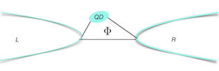
II.3 The particle and spin currents
Introducing the definition of the lesser Green’s function
| (11) |
(with similar definitions for the subscripts of all other Green’s functions that appear below), we can write the rate (4) in the left lead in the form
| (12) |
As the system is stationary, the Green’s functions depend only on the time difference. Hence, it is convenient to use the Fourier transforms (for all Green’s functions)
| (13) |
Exploiting relations (10), and using matrix notations (in spin space), Eq. (12) for the rate takes the form
| (14) |
where the superscript t on indicates the transposed matrix, and where
| (15) |
are matrices in spin space. These Green’s functions are derived in terms of the tunneling amplitudes and the Green’s functions of the decoupled system (which are denoted by lowercase letters); see Appendix A for the detailed calculation. We show there [Eq. (67)] that to lowest order in the tunneling amplitudes the rate (14) is
| (16) |
with the transmission matrix (in spin space),
| (17) |
Here, is the energy that scales the tunneling amplitudes (see Appendix B), is the density of states at the Fermi energy in the left (right) lead, and
| (18) |
where is the Green’s function of the decoupled dot, Eq. (54). The transmission matrix is obtained from Eq. (17) by replacing , and .
The particle current in the left lead is thus [see Eqs. (2) and (4)]
| (19) |
The particle current in the right lead, , is derived from Eqs. (18) and (19) by replacing and , which results in the transmission multiplied by . As , the particle currents obey , as required for charge conservation. This is not the case with the spin currents. The spin current in the left lead [Eqs. (3) and (16)] is
| (20) |
and the one in the right lead is derived from Eq. (20) by replacing and . Since in general [Eq. (18)] does not commute with , the spin currents in the two leads are not necessarily conserved (see Sec. III.1).
III Interference contributions to the transmission
As seen from Eqs. (17) and (18), the transmission matrix pertaining to the left lead comprises two parts. The first, , is independent of the Aharonov-Bohm flux,
| (21) |
It describes the transmission through the direct connection between the reservoirs, and the transmission through the arm carrying the quantum dot. The second part of the left-side transmission matrix (17), , is the interference contribution,
| (22) |
and that corresponding to the interference contribution of the right-side transmission reads
| (23) |
One observes that ; however, generally , indicating that while the particle current is conserved, generally, the spin current in the two leads is not [see Eqs. (19) and (20)]. It is interesting to compare the electronic paths that constitute and : Eq. (22) comprises paths that traverse the interferometer from the point and backwards (see Fig. 1), while contains the paths that start and end at the point .
III.1 Interference transport: effects of the Rashba interaction
Here we discuss the transmissions and the accompanying geometric phases in the case where the electrons on the interferometer are subjected solely to the Rashba interaction and the orbital Aharonov-Bohm flux. The tunneling amplitude pertaining to this situation is derived in Appendix B [see Eq. (84)]; it is found that in the absence of the Zeeman field the tunneling amplitudes are proportional to unitary matrices,
| (24) |
where sets the energy scale of the tunneling (assumed for simplicity to be the same on all edgescomm). Here, is the strength of the Rashba interaction (in momentum units), is the length of the corresponding edge of the triangle, with (see Fig. 1), and is a unit vector in the direction of the effective magnetic field induced by the Rashba interaction on an electron tunneling through the edge ,
| (25) |
Here, is a unit vector in the direction of the bond from to , and is the direction of the electric field creating the Rashba interaction. In our model is normal to the plane of the triangle, and is chosen to lie along the axis; hence all three vectors lie in the plane of the triangle, i.e. in the plane.
Given the explicit forms of the ’s in Eq. (24), we can now discuss the relations between the magnetization rates in the two leads, . Starting from Eq. (23), we find
| (26) |
where is an arbitrary unit vector. For , commutes with , and therefore
| (27) |
Substituting this relation in Eq. (20) yields
| (28) |
which means that the current of the spin component perpendicular to the bond in the interferometer plane is conserved. Note that in the absence of the Zeeman interaction does not contribute to the magnetization rates.
The situation is more complicated for the two other spin components, perpendicular to . These components do not commute (or anti-commute) with , and therefore they are not conserved. Indeed, a direct calculation using the commutator shows that is non-zero in the plane perpendicular to . This sum represents a magnetization which is injected into the two reservoirs. As we show in Appendix C, there are no simple relations between these components in the two reservoirs (except for the equilateral triangle). Within our low-order expansion in the tunneling amplitudes we neglect the effects of these polarizations on the electronic distribution functions in the reservoirs, Eq. (1). However, there will be some buildup of spin polarizations in the terminals near the interferometer, which might be detectable experimentally.
We next relate the particle and spin currents to the various angles and phases. As in the absence of the Zeeman field is just a number, it is clear that (note that ), which corresponds to a tunneling path from the left lead, around the triangle, back to the left lead, is also a unitary matrix, and has the general form
| (29) |
where is a real scalar and is a real vector, that has components in the plane of the triangle, , as well as a normal component, ,
| (30) |
Explicit expressions for these coefficients for an arbitrary triangle are given in Eq. (95). As seen from Eqs. (3), (16), and (22), the magnetization rate in the left lead (or the spin current associated with that lead) is along the vector [see also Eq. (48) below]. Therefore, we consider this vector as an effective magnetic field, induced by the spin-orbit interaction which generates this magnetization. The appearance of the component indicates that the effective magnetic field (which on each edge is in the plane of the triangle) attains a component when the amplitude along a path formed of several edges is followed. Interestingly, this component arises from the non-commutability of the tunneling matrices on the three triangle edges. Avishai We denote by the tilt-angle between this spin-orbit-induced magnetic field and the axis,
| (31) |
For a perfectly circular geometry, this angle is related to the Berry phase, or more generally to the Aharonov-Anandan phase, see e.g., Refs. Qian, Vanderbilt, and Frustaglia. As already mentioned, this is not true for the arbitrary triangular interferometer.
A priori, the right-to-right path requires the product
| (32) |
and consequently
| (33) |
On a physical basis, one expects that
| (34) |
as is indeed the case, since is a real number [see also Eq. (95)]. Explicitly, Eqs. (29) and (31) can be written as
where we denote . The spinor eigen vectors of the matrix in Eq. (III.1), whose corresponding eigen values are , are well-known,
It hence follows that
| (41) |
where
| (42) |
is the Aharonov-Casher phase. AC Due to the unitarity of the matrices in conjunction with Eq. (34), , the Aharonov-Casher phase acquired by the left-to-left path and the one accumulated on the right-to-right path, , are identical,
| (43) |
Therefore,
| (44) |
and hence
| (45) |
The interference part of the particle currents [Eq. (19)] is thus
| (46) |
There is no phase shift in , but measuring the amplitude of the periodic and symmetric Aharonov-Bohm oscillations in the magnetoconductance gives information about the Aharonov-Casher phase of the interferometer, via the coefficient . This observation was made a long time ago, Meir and was recently examined in great detail. Avishai
The spin current associated with the left lead is given by Eq. (20), with
| (47) |
which is parallel to the vector . Hence,
| (48) |
Similar to the calculation presented above, the magnetization rate in the right lead is given by
| (49) |
which is along . From Eq. (28) it then follows that , but there exists no obvious relation between the transverse components in the two reservoirs, and thus no relation between the angles and .
Several conclusions can be drawn from the expressions for the interference-induced parts of the currents. The conspicuous one is that measuring the interference parts of the currents in an arbitrarily-shaped Aharonov-Bohm interferometer in the absence of a Zeeman field gives unambiguously only the Aharonov-Casher AC geometric phase . Unlike the case of the circular loop, Qian; Frustaglia it is not clear if and how measurements of the tilting angles and can yield information about the Aharonov-Anandan (or the Berry) or the dynamic phases.
III.2 Interference transport: joint effects of spin-orbit and Zeeman interactions
When the tunneling electrons are subjected to the Zeeman interaction alone then [see Appendix C, in particular Eqs. (94) and (100)]
| (50) |
where and are real expressions comprising , , and . Here, is the length of the bond , see Fig. 1, is the Green’s function of the decoupled dot [given in Eqs. (54) and (87)], and is derived in Appendix B ( is the localization radius in the barrier Shahbazyan and is the effective mass). It follows that the transmissions and [Eqs. (22) and (23), respectively] are identical, and are proportional to . Obviously, the interference-induced parts of the charge conductance and the magnetization rates have solely the dependence; the magnetization rates are only along , the direction of the Zeeman field. Both the charge and the spin currents are conserved. One also notes that the oscillatory dependence on the lengths of the bonds, resulting from the Rashba interaction, is totally lost in this case (it is replaced by a combination of hyperbolic functions).
The presence of both the spin-orbit and the Zeeman interactions modifies the results reported in Sec. III.1. Since the pertaining expressions are relatively cumbersome, and in any event depend heavily on geometric details, they are relegated to Appendix C. Here we summarize the qualitative results. We begin with the interference contribution to the charge conductance. Let us first ignore the Zeeman interaction on the decoupled dot and keep this interaction only in the tunneling amplitudes. Then from Eq. (99) we find that there are real contributions to , which are second order in , with comim , see Appendix B. Consequently, these terms are multiplied by . These additional contributions to the charge conductance modify the coefficient of in Eq. (46) but do not change it in any essential way; they do change the period of the oscillations with the lengths . t0
The effect of the terms in which are first order in is very different. Since they lead to one of our main results, we reproduce them here. From Eq. (99), the contributions to the scalar part are
| (51) |
As seen, the contributions of the terms in Eq. (51) to the charge conductance are multiplied by , making the expression even in the magnetic field, but not periodic. For example, confining ourselves to an equilateral triangle, we find that Eq. (46) changes to
| (52) |
where . The authors of Refs. Peeters and Lyanda expressed the conductance as a sum of two contributions (from the two spin directions), each of which is a periodic function in the Aharonov-Bohm flux with its own phase shift that depends on the Zeeman field. In Ref. Peeters that phase shift is related to the Aharonov-Casher phase of the interferometer, while that of Ref. Lyanda is claimed to be the Berry phase. As seen, our result is generally not related neither to the tilting angles or discussed in Sec. III.1, nor to the Aharonov-Casher phase. In this respect our result is also different from the one of Ref. Ady, derived for a system subjected to a Zeeman field perpendicular to the loop and another, time-dependent magnetic field which rotates in the plane of the loop: the expression for the conductivity presented there contains only terms.
Next we discuss what modifications the Zeeman interaction on the dot may introduce. As shown in Appendix C, apart from real terms whose contribution to the charge conductance is multiplied by , there appear also terms of the type presented in Eq. (51), with replaced by . This implies that the Zeeman interaction on the dot alone, in conjunction with the spin-orbit interaction in the tunneling amplitudes, suffices to induce the dependence of the Aharonov-Bohm oscillations alluded to above. Strictly speaking, one expects that when the dot is far from resonance (as assumed in our model).
The effect of the Zeeman interaction on the magnetization rates is discussed in the second part of Appendix C. Since the magnetization rate is expected to be odd in the magnetic field, it is not surprising that the terms which are linear in the Zeeman field contribute only terms proportional to to the magnetization rates.
IV conclusions and discussion
We have analyzed the effects of the Rashba spin-orbit and Zeeman interactions on the flux dependence of the charge and spin transport through Aharonov-Bohm interferometers. We find that the Zeeman interaction, which is often ignored in the calculations, causes crucial qualitative changes in the results, which should be observable.
Most of the earlier literature concentrated on circular loops, found relations among the geometric Aharonov-Casher, Aharonov-Anandan and dynamic phases, and considered possibilities to extract these phases from experiments. We find that the circular configuration is probably unique, and simple relations seem not to exist for other shapes of the loop. To demonstrate this point we calculated the charge and spin currents through a triangular loop, to lowest order in the tunneling amplitudes.
The spin-orbit interaction is known to generate an effective spin-dependent vector potential, so that a spin which moves around a loop accumulates the Aharonov-Casher phase . When this interaction is added to the Aharonov-Bohm interferometer (but without the Zeeman field), we find that the leading interference contribution to the total magnetoconductance of the interferometer (coupled to unpolarized leads) is proportional to , and the only way to extract is to study the amplitude of the terms. No other phase (e.g., Aharonov-Anandan or Berry) can be extracted from such measurements.
The spin-orbit interaction, even without the Zeeman interaction, also generates interesting spin currents in the leads, whose amplitudes are all proportional to . Thus, measuring these currents again yields only the phase . While the current of the spin component in the plane of the triangle, perpendicular to the edge which connects the terminals directly, is conserved, the spin-orbit interaction on the interferometer generates a growing magnetization of the other two spin components in the two terminals. In general, these magnetizations have different tilt angles and with the axis perpendicular to the interferometer plane and different projections on the interferometer plane. These directions depend on the detailed structure of the triangular loop. We found no simple relation between the tilt angles and the Aharonov-Casher phase , or with any other “standard" phases. In fact, Vanderbilt Vanderbilt calculated the Berry phase for an equilateral triangle and for a regular edge polygon (Exercise 3.1.2 in Ref. Vanderbilt), and found that it can be characterized by a single tilt angle . His result reduces in the limit to the circular loop result . However, the expression for the Berry phase pertaining to a finite regular polygon is more complex, and clearly all these phases depend on the details of structure of the interferometer loop.
Adding a Zeeman field perpendicular to the interferometer plane breaks the unitarity of the tunneling amplitudes on the interferometer edges, and therefore also on the amplitude of a spinor after it goes around the loop. For a non-unitary matrix, one can no longer use the concept of the Aharonov-Casher phase. Indeed, we find that the amplitude of the function in the total magnetoconductance is modified by a term which depends on the Zeeman field. To obtain the pure spin-orbit Aharonov-Casher phase one has to extrapolate this amplitude to zero field. Furthermore, the combination of the spin-orbit interaction and the Zeeman field generates a new term in the magnetoconductance, which is proportional to . If one could treat the Zeeman field and the Aharonov-Bohm flux as two independent parameters of the problem, which can be fixed separately, then one could interpret this term as generating a phase shift in , proportional to . However, in practice both the Aharonov-Bohm flux and the Zeeman interactions arise due to the same external magnetic field, and . The resulting magnetoconductance is no longer a periodic function, but it remains an even function of the field. Since the phase results only from the normal component of the field, it may be interesting to consider rotations of the field away from this normal direction. For symmetry reasons, we expect the magnetoconductance of any interferometer to have the aperiodic but even form , with corrections of order in each coefficient , with a similar odd analog for the spin currents.
Acknowledgements.
This research was partially supported by the Israel Science Foundation (ISF), by the infrastructure program of Israel Ministry of Science and Technology under contract 3-11173, and by the Pazy Foundation. We acknowledge the hospitality of the PCS at IBS, Daejeon, Korea, where part of this work was done, under IBS funding number (IBS-R024-D1).Appendix A The Green’s functions’ calculation
The Green’s functions are derived from the corresponding Dyson’s equations, in terms of the tunneling amplitudes and the Green’s functions of the decoupled system (which are denoted by lowercase letters). The Green’s functions of the decoupled reservoirs are independent of the spin indices,
| (53) |
and that of the decoupled dot is diagonal in spin space
| (54) |
(it is assumed that the decoupled dot is empty). The lesser superscript is omitted, as the Dyson equations are valid for the three Keldysh Green’s functions, lesser, retarded and advanced; these are found by using Langreth rules Langreth for the analytic continuation on the time contour. Jauho
The Dyson equations for and [see Eqs. (15)], which involve the Green’s function , are (in spin space)
| (55) |
The integrand in the rate Eq. (14) is the lesser Green’s function , where , using Eqs. (55), is
| (56) |
Here we have introduced the notations
| (57) |
(In the main text we present in dimensionless units.) Notice that is a real matrix and consequently . The Dyson equation for can be written in two equivalent forms
| (58) |
Inserting Eqs. (55) then gives
| (59) |
From Eqs. (59) we find
| (60) |
Inserting these expressions into Eq. (56) yields
| (61) |
where the final equality results from the fact that is proportional to the unit matrix. The Dyson equations for and [Eqs. (15)] are
| (62) |
Inserting Eqs. (55) into Eqs. (62) and then using Eqs. (60), gives
| (63) |
Thus, the final expression is , with
| (64) |
where
| (65) |
and similarly for .
Appendix B Tunneling amplitude
Our derivation of the tunneling amplitude of an electron through a potential barrier is based on the one given in Ref. Shahbazyan. These authors considered an electron subjected to the linear Rashba spin-orbit interaction. Bychkov In Ref. com1 we extended their treatment to include the effect of the Zeeman interaction, for the case where the Fermi energy of the electrons in the leads exceeds the energy of the potential barrier. Here we consider the opposite situation, where the energy of the tunneling electron within the tunneling region is negative. This case was studied in Ref. Shahbazyan; we extend that study to include the Zeeman interaction, for a Zeeman field perpendicular to the tunneling link and to the magnetic field induced by the spin-orbit interaction. Adopting units in which , the Hamiltonian of an electron in the tunneling region is
| (68) |
where is the vector of the Pauli matrices, and is the coordinate along the tunneling path (assumed below to be on a straight line in the plane). In Eq. (68), is the vector potential, chosen to be along the direction of , is the (effective) mass, is the direction of the electric field creating the spin-orbit interaction, whose strength is in momentum units, and is the external magnetic field (in energy units), which is along the direction.
For a plane-wave solution with a wave vector directed along , the magnetic field induced by the spin-orbit interaction is
| (69) |
This effective magnetic field depends on the direction of , that is, on the direction of . For along the direction, and is a unit vector in the plane. The vector potential , which represents the orbital effect of the magnetic field, can be gauged out from the Hamiltonian, to reappear as the Aharonov-Bohm phase factor multiplying the tunneling amplitude (see the main text); hence it is ignored in the following. The spin-dependent propagator (i.e., the retarded Green’s function) is a 22 matrix in spin space. When the energy of the tunneling electron is negative (i.e., the Fermi energy in the leads is smaller than the potential barrier representing the tunneling region) then , where measures the extent of the localized wave function. Shahbazyan The tunneling amplitude, i.e., the propagator , is
| (70) |
where
| (71) |
The integral in Eq. (70) is evaluated by the Cauchy theorem, for the case where the coordinate is along a straight line, assuming that ,
| (72) |
Here, and are the roots of the denominator,
| (73) |
where
| (74) |
Focusing on the case , we introduce the variables and
| (75) |
which obey
| (76) |
and therefore
| (77) |
In terms of these variables, the scalar part of the expression on the right hand-side of Eq. (72) is
| (78) |
the part is
| (79) |
and the part related to is
| (80) |
Adopting the plausible assumption that is larger than the spin-orbit and the Zeeman energies,
| (81) |
we find that
| (82) |
The propagator is then
| (83) |
In the main text we replace the prefactor of by , ignoring for simplicity its dependence on the length of the bond, i.e. .comm
In the limit of zero Zeeman field , Eq. (83) for the propagator reduces to
| (84) |
This unitary form is the one expected when only the spin-orbit interaction is active. Meir On the other hand, when there is only the Zeeman field and is purely imaginary, the propagator is
| (85) |
where
| (86) |
[Note that , see Eqs. (81).] In this case the oscillations as a function of the distance , which are essentially due to the spin-orbit interaction, are absent. In fact, they disappear once (the Zeeman energy divided by the energy at the barrier, ) exceeds the spin-orbit energy.
Appendix C The interference terms in the transmission of a triangular interferometer
Here we consider the interference contributions to the transmission matrices, and [Eqs. (22) and (23), respectively] in the presence of both the Rashba and the Zeeman interactions. In this case, the tunneling amplitude of each bond is given by Eq. (83), and is not proportional to a unitary matrix as in the presence of the spin-orbit interaction alone; the Zeeman interaction also changes the Green’s function of the decoupled dot, , into a matrix, since by Eq. (54)
| (87) |
Below, we first ignore the Zeeman interaction on the dot [i.e., we assume that ] and consider only the product [see e.g., Eq. (22)]; we then investigate this product when the term in Eq. (87) is accounted for.
To consider the product for an arbitrary triangular interferometer, it is convenient to introduce the shorthand notations
| (88) |
In the absence of the Zeeman field and , while when there is no spin-orbit interaction , is purely imaginary, and [see Eqs. (82)]. With these notations,
| (89) |
where
| (90) |
Explicitly,
| (91) |
| (92) |
and
| (93) |
In the absence of the spin-orbit interaction,
| (94) |
where is given in Eq. (86) and . In this case is a real matrix, invariant under ; as a result, the charge conductance and the magnetization rates are proportional to ,, and they are both conserved. In the absence of the spin-orbit interaction, the magnetization rates are solely along the axis, that is, along the direction of the Zeeman field.
In the absence of the Zeeman interaction
| (95) |
This case is discussed in great detail in Sec. III.1. Equating Eq. (95) to Eq. (29) yields
| (96) |
Projecting on confirms Eq. (28). Projections on the transverse directions does not yield simple relations between the transverse magnetization rates of the two reservoirs. An exception is the equilateral triangle, for which
| (97) |
and therefore
| (98) |
In this special case we find that , hence . Setting yields .
Returning to the case where both spin-orbit and Zeeman interactions are present in the tunneling amplitude, we first ignore the effect of the Zeeman interaction on the dot and examine the scalar part of the product (which determines the charge conductance), that is
| (99) |
Here we find a dramatic difference as compared to the case where the Zeeman interaction is absent: the appearance of the last term on the right hand-side of Eq. (99). As shown in Sec. III.2, this term modifies the Aharonov-Bohm oscillations of the magnetoconductance as a function of the flux , which now acquire an additional dependence upon . The amplitude of the latter is proportional to the Zeeman field (and thus the result is compatible with the Onsager relations) and vanishes in the absence of the spin-orbit coupling.
Adding the Zeeman energy to the Green’s function of the decoupled dot [see Eq. (87)] and expanding to linear order in , yields
| (100) |
where the tunneling amplitudes in the last term on the right hand-side of Eq. (100) should be considered for , i.e., they are given by Eqs. (24). Then, noting that , leads to
| (101) |
which implies that we need the product . The latter is given in Eq. (95) with replaced by . The resulting contribution from the Zeeman energy in the Green’s function of the dot to the scalar part of Eq. (100) then comes from the terms of the form in Eq. (95). Multiplying such a term by contributes to the scalar part an imaginary term , which is similar to the contribution of the Zeeman interaction in the tunneling amplitudes [i.e., the last term in Eq. (99)], except that its coefficient now contains instead of . These add to the term in the charge conductance, in the same way as the last term Eq. (99). When the dot is far from resonance, these contributions are smaller (note that our analysis is not strictly valid when the dot is close to resonance).
Turning now to the terms yielding the magnetization rates, we focus on those linear in the Zeeman field. There are two types of such terms. First, there are those linear in that are included in Eqs. (89)-(93). These should be multiplied by [see, e.g., Eq. (20)] and then traced over. An examination of Eqs. (89)-(93) shows that they yield
| (102) |
for the magnetization rate along an arbitrary unit vector . As seen, the first two terms on the right hand-side of Eq. (102) contribute only to the magnetization rates along , and that contribution is real. As a result, they give rise to a dependence in . The last expression on the right hand-side of Eq. (102) necessitates the product , where the vector , which denotes the circular brackets, lies in the plane. Therefore, terms of this type contribute only to the in-plane magnetization rates, , and that contribution which is real, also leads to a dependence of the magnetization rates.
The second type of contributions comes from the Zeeman interaction in the Green’s function on the dot. Exploiting Eqs. (100) and (101) and the definition (20) implies that the expression for the magnetization rates along the unit vector due to those comprises terms of the form
| (103) |
As at , . From Eq. (95), and are real, and therefore the contributions of the Zeeman interaction to the magnetization rates are real, generating terms proportional to . Thus, all magnetization rates due to the Zeeman interaction, of order or , have coefficients which are even functions of . This is not surprising: the magnetization rates are expected to be odd functions of the magnetic fields. Note that the magnetization rates due to the spin-orbit interaction alone, Eq. (47), all have a dependence.
References
- (1) Y. Aharonov and A. Casher, Topological quantum Effects for Neutral Particles, Phys. Rev. Lett. 53, 319 (1984).
- (2) Y. Aharonov and D. Bohm, Significance of Electromagnetic Potentials in the Quantum Theory, Phys. Rev. 115, 485 (1959).
- (3) E. I. Rashba, Properties of semiconductors with an extremum loop .1. Cyclotron and combinational resonance in a magnetic field perpendicular to the plane of the loop, Fiz. Tverd. Tela (Leningrad) 2, 1224 (1960) [Sov. Phys. Solid State 2, 1109 (1960)]; Y. A. Bychkov and E. I. Rashba, Oscillatory effects and the magnetic susceptibility of carriers in inversion layers, J. Phys. C 17, 6039 (1984).
- (4) J. Nitta, T. Akazaki, H. Takayanagi, and T. Enoki, Gate Control of Spin-Orbit Interaction in an Inverted In0.53Ga0.47As/In0.52Al0.48As Heterostructure, Phys. Rev. Lett. 78, 1335 (1997).
- (5) T. Bergsten, T. Kobayashi, Y. Sekine, and J. Nitta, Experimental Demonstration of the Time Reversal Aharonov-Casher Effect, Phys. Rev. Lett. 97, 196803 (2006).
- (6) T-Z. Qian and Z-B. Su, Spin-Orbit Interaction and Aharonov-Anandan Phase in Mesoscopic Rings, Phys. Rev. Lett. 72, 2311 (1994).
- (7) M. V. Berry, Quantal phase factors accompanying adiabatic changes, Proc. Royal Soc. A 392, 45 (1984).
- (8) D. Vanderbilt, Berry Phases in Electronic Structure Theory: Electric Polarization, Orbital Magnetization and Topological Insulators, Cambridge University Press (2018).
- (9) Y. Aharonov and J. Anandan, Phase Change during a Cyclic Quantum Evolution, Phys. Rev. Lett. 58, 1593 (1987).
- (10) D. Loss, P. Goldbart, and A. V. Balatsky, Berry’s Phase and Persistent Charge and Spin Currents in Textured Mesoscopic Rings, Phys. Rev. Lett. 65, 1655 (1990).
- (11) S. Oh and C-M. Ryu, Persistent spin currents induced by the Aharonov-Casher effect in mesoscopic rings, Phys. Rev. B 51, 13441 (1995).
- (12) M. Ellner, N. Bolivar, B. Berche, and E. Medina, Charge- and spin-polarized currents in mesoscopic rings with Rashba spin-orbit interactions coupled to an electron reservoir, Phys. Rev. B 90, 085305 (2014).
- (13) Y. Avishai, K. Totsuka, and N. Nagaosa, Non-Abelian Aharonov-Casher Phase Factor in Mesoscopic Systems, J. Phys. Soc. Jpn. 88, 084705 (2019).
- (14) Y. Meir, Y. Gefen, and O. Entin-Wohlman, Universal effects of spin-orbit scattering in mesoscopic systems, Phys. Rev. Lett. 63, 798 (1989).
- (15) J. Nitta, F. E. Meijer, and H. Takayanagi, Spin-interference device, Appl. Phys. Lett. 75, 695 (1999).
- (16) B. Molnár, F. M. Peeters, and P. Vasilopoulos, Spin-dependent magnetotransport through a ring due to spin-orbit interaction, Phys. Rev. B. 69, 155335 (2004).
- (17) D. Frustaglia and K. Richter, Spin interference effects in ring conductors subject to Rashba coupling, Phys. Rev. B 69, 235310 (2004).
- (18) R. Capozza, D. Giuliano, P. Lucignano, and A. Tagliacozzo, Quantum Interference of Electrons in a Ring: Tuning of the Geometrical Phase, Phys. Rev. Lett. 95, 226803 (2005).
- (19) J-B. Yau, E. P. De Poortere, and M. Shayegan, Aharonov-Bohm Oscillations with Spin: Evidence for Berry’s Phase, Phys. Rev. Lett. 88, 146801 (2002).
- (20) M. König, A. Tschetschetkin, E. M. Hankiewiccz, J. Sinova, V. Hock, V. Daumer, M. Schaefer, C. R. Becker, H. Buhmann, and L. W. Molenkamp, Direct Observation of Aharonov-Casher Phase, Phys. Rev. Lett. 96, 076804 (2006).
- (21) F. Nagasawa, J. Takagi, Y. Kunihashi, M. Kohda, and J. Nitta, Experimental Demonstration of Spin Geometric Phase: Radius Dependence of Time-Reversal Aharonov-Casher Oscillations, Phys. Rev. Lett. 108, 086801 (2012).
- (22) A. G. Aronov and Y. B. Lyanda-Geller, Spin-Orbit Berry Phase in Conducting Rings, Phys. Rev. Lett. 70, 343 (1993).
- (23) F. E. Meijer, A. F. Morpurgo, and T. M. Klapwijk, One-dimensional ring in the presence of Rashba spin-orbit interaction: Derivation of the correct Hamiltonian, Phys. Rev. B 66, 033107 (2002).
- (24) Y-S. Yi, T-Z. Qian, and Z-B. Su, Spin precession and time-reversal symmetry breaking in quantum transport of electrons through mesoscopic rings, Phys. Rev. B 55, 10631 (1997).
- (25) O. Entin-Wohlman, A. Aharony, Y. Tokura, and Y. Avishai, Spin-polarized electric currents in quantum transport through tubular two-dimensional electron gases, Phys. Rev. B 81, 075439 (2010).
- (26) As seen in Appendix C, the dependent terms are all proportional to the product of the three ’s.
- (27) D. C. Langreth, Linear and nonlinear response theory with applications, in Linear and Nonlinear Electron Transport in Solids, eds. J. T. Devreese and E. van Boren (Plenum, New York, 1976).
- (28) A. P. Jauho, Nonequilibrium Green function modelling of transport in mesoscopic systems, in Progress in Nonequilibrium Green’s Functions II, eds. M. Bonitz and D.Semkat (World Scientific, Singapore, 2003).
- (29) T. V. Shahbazyan and M. E. Raikh, Low-Field Anomaly in 20 Hopping Magnetoresistance Caused by Spin-Orbit Term in the Energy Spectrum, Phys. Rev. Lett. 73, 1408 (1994).
- (30) A. Aharony, O. Entin-Wohlman, M. Jonson, and R. I. Shekhter, Electric and magnetic gating of Rashba-active weak links, Phys. Rev. B 97, 220404(R) (2018), see also Supplemental Material at http://link.aps.org/supplemental/10.1103/PhysRevB.97.220404
- (31) Note that always appears in the terms of Eq. (99) in conjunction with , and hence all terms in Eq. (99) are real except for those that are explicitly multiplied by .
- (32) In the presence of the Zeeman interaction, the independent part of the transmission, , also contributes terms of order to the conductance.
- (33) A. Stern, Berry’s Phase, Motive Forces, and Mesoscopic Conductivity, Phys. Rev. Lett. 68, 1022 (1992).