Linear Stochastic Dividend Model
Abstract
In this paper we propose a new model for pricing stock and dividend derivatives. We jointly specify dynamics for the stock price and the dividend rate such that the stock price is positive and the dividend rate non-negative. In its simplest form, the model features a dividend rate that is mean-reverting around a constant fraction of the stock price. The advantage of directly specifying dynamics for the dividend rate, as opposed to the more common approach of modeling the dividend yield, is that it is easier to keep the distribution of cumulative dividends tractable. The model is non-affine but does belong to the more general class of polynomial processes, which allows us to compute all conditional moments of the stock price and the cumulative dividends explicitly. In particular, we have closed-form expressions for the prices of stock and dividend futures. Prices of stock and dividend options are accurately approximated using a moment matching technique based on the principle of maximal entropy.
1 Introduction
In recent years there has been an increased interest in trading dividend derivatives, in particular dividend futures. Since there also exists an active market for derivatives referencing the price of the stock paying the dividends, there is a need for derivative pricing models that can jointly price derivatives on the stock and on the dividends. Since dividend derivatives typically reference the nominal amount of dividends paid over a window of time, it seems natural to directly specify tractable dynamics for the dividend payments, or the dividend rate if dividends are paid out continuously, under a risk-neutral measure. The challenging part of this approach is to keep the stock price positive. Indeed, in absence of arbitrage and frictions such as taxes, the stock price must decrease by exactly the amount paid out as dividend, which can push the stock price in negative territory if no connection is made between the dividend and stock price dynamics. An easy solution to this problem is to model dividend yields, i.e., the fraction of the stock price that is paid out as a dividend, instead of dividends themselves. However, such a choice complicates the valuation of dividend derivatives, since their payoff now involves the product between the stock price and the dividend yield.
In this paper, we consider a stock that pays out dividends continuously11 1 In reality, dividends are paid out discretely instead of continuously. Most liquid dividend derivatives, however, reference dividends paid by a stock index, in which case continuously paid dividends are considered an acceptable approximation. at a rate that is stochastically varying over time. The dividend rate is defined as a linear function of a multivariate factor process that belongs to the class of of polynomial diffusions, see e.g. Filipović and Larsson 2016. The drift and martingale part of the factor process and the martingale part of the stock price process are specified such that the dividend rate is non-negative and upper bounded by a constant fraction of the stock price. As a consequence, the dividend rate will go to zero as the stock price goes to zero, which guarantees the non-negativity of the stock price. The dividend yield process therefore has a zero lower bound and an upper bound that can be chosen arbitrarily large. We show that the zero boundary of the stock price is always unattainable and we provide parameter restrictions for boundary non-attainment of the factor process. The dynamics of the model becomes most intuitive with a one dimensional factor process. In this case, the dividend rate is mean-reverting around a constant fraction of the stock price. Long-term dividend futures therefore behave proportional to the stock price, while short term dividend futures have dynamics of their own. In particular, this allows to have low volatility in short-term dividend futures, while long-term dividend futures inherit the relatively high volatility of the stock price. As highlighted by Buehler 2018, this is a desirable feature for stochastic dividend models. Since the model belongs to the class of polynomial processes, we can compute all moments of the stock price and the (integrated) dividend rate in closed-form. In particular, this means we have closed-form prices for stock and dividend futures. Prices of stock and dividend options are efficiently approximated using a moment-matching technique based on the principle of maximal entropy, similarly as in Filipović and Willems 2018. In a numerical study we show that option prices are approximated accurately with a small number of moments.
We show that our model does not contain a bubble in the sense that the discounted gains process is a true martingale and that the stock price is equal to the present value of all future dividends. It is important to note that the latter is not necessarily true in an arbitrage free model. Indeed, even if the discounted gains process is a true martingale, absence of arbitrage only guarantees that the present value of all future dividends is lower than or equal to the stock price. The difference between the two is equal to the present value of the stock price at an infinite time horizon, which we show to be zero in our model. This property distinguishes our model from the one of Buehler 2018, where the dividend rate is mean-reverting around the present value of the stock price at infinity.
The literature on dividend derivative pricing is relatively scarce. Buehler et al. 2010 proposes a model where the stock price jumps at known dividend payment dates and follows log-normal dynamics in between the payment dates. The jump amplitudes are driven by an Ornstein-Uhlenbeck process such that the stock price remains log-normally distributed and the model has closed-form prices for European call options on the stock. Dividend derivatives, however, have to be priced with Monte-Carlo simulations. In order to reconcile the high volatility in the stock price with the low volatility in dividends, they use a very negative () correlation between the process driving the jump amplitudes and the stock price. An important drawback of their approach is that dividend payments are not guaranteed to be non-negative. Tunaru 2018 uses a similar setup as Buehler et al. 2010, but uses a beta distribution for the jump amplitudes. The choice for a compactly supported jump distribution guarantees non-negative dividend payments. However, the diffusive noise of the stock has to be assumed independent of the jump amplitudes in order to have tractable expressions for dividend futures prices. Smoothing the dividends through a negative correlation between stock price and the jump amplitudes, as in Buehler et al. 2010, is therefore not possible. In a second approach, Tunaru 2018 directly models the cumulative dividends with a logistic diffusion model. The latter has however no guarantee to be monotonically increasing, meaning that negative dividends occur frequently. Moreover, the model must be reset on an annual basis. Option pricing is done using Monte-Carlo simulation for both methods in Tunaru 2018. Buehler 2018 decomposes the stock price as the sum of a fundamental component, representing the present value of all future dividends, and a residual bubble component. The dividends are driven by a process that mean-reverts around the bubble component. The aim of this setup is to capture the stylized fact that long-term dividend futures tend to move together with the stock price, while short-term dividend futures are much less volatile. Our model, in its simplest form, shares some similarities with the approach of Buehler 2018. However, instead of modeling the dividends as mean-reverting around a bubble component, we choose to make them mean-revert around the stock price itself, which seems more intuitive and leads directly to the desired positive correlation between long-term dividend futures and the stock price. Guennoun and Henry-Labordere 2017 consider a stochastic local volatility model for the pricing of stock and dividend derivatives. Their model guarantees a perfect fit to observed option prices, however all pricing is based on Monte-Carlo simulations. Filipović and Willems 2018 introduce a framework based on polynomial jump-diffusions to jointly price interest rate, dividend, and stock derivatives. Our model is a special case of their general framework, but is different from the Linear Jump-Diffusion model (LJD) that was used in the numerical study of Filipović and Willems 2018.
The model proposed in this paper also shares some similarities with the linear hypercube model model of Ackerer and Filipović 2019 in the context of credit risk. Specifically, they specify a survival process whose drift is a linear function of a diffusive factor process with linear drift. In order for the survival process to be positive and non-increasing, they specify the factor process such that its components are all non-negative and upper bounded by the survival process. In our setup, the dividend rate is a linear function of a diffusive factor process with linear drift, which has to be specified such that the stock price is positive and the dividend rate non-negative. The stock price, whose drift is linear in the dividend rate, therefore plays a similar role as the survival process in Ackerer and Filipović 2019, but with the important difference that the stock price has a martingale part while the survival process is absolutely continuous. This martingale part requires special care and, in particular, rules out the factor process specification of the linear hypercube model of Ackerer and Filipović 2019.
The remainder of this paper is structured as follows. Section 2 specifies the model dynamics. Section 3 discusses the pricing of stock and dividend derivatives. In Section 4 we calibrate a parsimonious model specification to market data. Section 5 presents an extension of the model with jumps in the stock price. Section 6 concludes. All proofs are collected in the appendix.
2 Model specification
Let denote the stock price process and the instantaneous dividend rate. Suppose for simplicity that interest rates are constant. Consider the following dynamics for under a risk-neutral measure
| (1) | ||||
| (2) | ||||
| (3) |
where is the short-rate, , is a -dimensional factor process, , , , , and is a -dimensional standard Brownian motion. The following proposition provides parameter conditions such that (2)-(3) admits a unique solution taking values in
Proposition 2.1.
We henceforth assume that the inequalities in (4) and (5) are satisfied and . The above proposition shows in particular that we have and for all . The condition in (6) can be used to bound strictly away from zero, although this is not required from an economic point of view. The diffusive term of is specified such that it vanishes at the boundary , which is necessary to keep the process inside . The condition in (7) can be used to bound the stock price volatility strictly away from zero.
Remark 2.2.
Remark that the more general specification , for some , is equivalent to the one in (1). Indeed, if we define with , then we can write . The dynamics of are of the same form as the dynamics of
with , , and , .
If we define the dividend yield , then we have
The dividend yield is therefore bounded from above by a parameter of our choice. The dynamics of the log-price is given by
The volatility of the log-price process therefore depends on the dividend yield. There is empirical evidence that dividend payout policies affect stock price volatility, see e.g. Baskin 1989, which is consistent with the dynamics of this model. In case this is not desirable, the influence of the dividend yield on the log-price volatility can be made arbitrarily small by choosing large enough.
The following proposition shows that our model does not contain a bubble in the stock price dynamics.
Proposition 2.3.
The discounted gains process is a martingale. If , then we have for all
| (8) |
Equation (8) shows that the stock price is equal to the present value of all future dividends in our model. It is important to note that this is not a trivial relationship. Indeed, from no-arbitrage principles, it only follows that the present value of future dividends must be lower than or equal to the stock price, see e.g. Filipović and Willems 2018. In general, if the discounted gains process is a martingale, then
A positive difference between the stock price and the present value of future dividends can be interpreted as the present value of a terminal payment at an infinite time horizon, which is difficult to reconcile with standard economic theory. Proposition 2.3 shows that, in our model, we have if . The derivation of this result relies on the linear drift structure of and the geometry of , which are a key ingredients of our model. In Example 2.5 in the next section, we illustrate a parameterization where the assumption is violated and (8) does not hold.
Remark 2.4.
The processes and have zero quadratic covariation. Note that this does not mean that dividends are independent of the stock price, since still enters in the drift and diffusion function of . The dynamics of can be generalized to allow for non-zero quadratic covariation with as follows
for some parameters , . All the results in the paper are easily adjusted to accommodate this generalization.
2.1 Single factor model
For , we obtain the following model dynamics
| (9) | ||||
| (10) |
If , then is mean-reverting around , with an upper bound of . The inward pointing drift conditions (4) and (5) become
| (11) |
Boundary non-attainment is satisfied if and
The dividend yield becomes an autonomous diffusion with the following dynamics
Remark that the dividend yield process is not a polynomial diffusion, due to the terms and in the drift, and and in the diffusion function. However, since is typically in the order of percentage points, higher powers of contribute relatively little to the dynamics. In particular, the dividend yield has approximately a linear drift .
We end this section with an example where the assumption in Proposition 2.3 is violated.
Example 2.5.
If , then we have for all , and (11) becomes . The present value of future dividends is
Using and we obtain
The present value of future dividends is therefore lower than or equal to the stock price, as required by absence of arbitrage. If or , then we have an example where the present value of future dividends is strictly below the stock price, i.e., does not go to zero as .
The above example shows that the presence of in the drift of is crucial for the stock price to be equal to the present value of future dividends.
3 Derivative pricing
In this section we show how to compute prices of derivatives referencing the stock price and/or the dividends paid over some time interval.
3.1 Moments of stock price and cumulative dividends
Define the cumulative dividend process as
which represents all the dividends paid out over a time interval . In contrast to the instantaneous dividend rate , the cumulative dividend is observable in practice. The process is jointly a polynomial diffusion, so we are able to compute all conditional moments in closed form, see e.g. Filipović and Larsson 2016 for details. Let denote the set of polynomials with . Applying the infinitesimal generator of to a twice differentiable function gives
where the subscripts of denote partial derivatives, the gradient of , and we have omitted the function arguments for brevity. It is easily verified that for any . Therefore, if we fix a vector of polynomial basis functions for , with , then we can find a unique matrix such that for all
By definition of the infinitesimal generator, we obtain the following moment formula
| (12) |
In particular, we can compute all the -conditional mixed moments of in closed form for all .
Remark 3.1.
If one is only interested in the moments of , then there is no need to augment the state with , since is already a polynomial diffusion on its own.
3.2 Linear derivatives
For , we can without loss of generality choose the basis . The matrix then becomes
The most actively traded linear derivatives are stock futures and dividend futures. Stock futures settle on the stock price at some terminal date and dividend futures settle on the dividends paid in a time interval . The moment formula (12) can be used to compute prices of stock futures and dividend futures. Indeed, futures prices are given by the risk-neutral expectation of the terminal settlement price because of continuous marking-to-market, so we get
| (13) | ||||
| (14) |
where denotes the -th canonical basis vector in , , and . In case the reference period of the dividend futures has already started, i.e., , we get
| (15) |
Without loss of generality we can assume that , in which case and is the amount of dividends already paid.
Remark that the volatility parameters and do not enter into the prices of dividend futures, which is a consequence of the linear drift structure of . This allows us, for example, to calibrate and to dividend futures first, and subsequently use and to calibrate non-linear derivatives such as stock and dividend options. The parameter also does not appear in the prices of dividend futures, however it should be noted that the value of affects the values that and are allowed to take, because of the inequalities (4) and (5) that we assume to be true.
3.3 Non-linear derivatives
Consider a derivative on the stock price with discounted payoff at time given by , for some function . In absence of arbitrage, its price at time is given by
The probability density function of is not known explicitly, so we cannot compute by direct integration in general. We do however know all the moments of through the moment formula (12). In particular, if is a polynomial, then we can compute explicitly. If is not a polynomial, we approximate using the available stock price moments and the principle of maximum entropy, similarly as in Filipović and Willems 2018. Specifically, denote by , , the first moments of the stock price. We now look for a probability density function which has the same first moments as and has maximal entropy:
| (16) |
where we set so that the density integrates to one. Jaynes 1982 motivates such a choice by noting that maximizing entropy incorporates the least amount of prior information in the distribution, other than the imposed moment constraints. In this sense it is maximally noncommittal with respect to unknown information about the distribution. Straightforward functional variation with respect to gives the following unique solution to the optimization problem in (16)
where the Lagrange multipliers have to be solved numerically from the moment constraints. Finally, we approximate by numerically computing the integral
We can use exactly the same approach to price dividend derivatives with discounted payoff at time given by , for some function . All we need are the moments of , which can be computed explicitly using the law of iterated expectations and the moment formula (12) as follows
where and are the unique vectors satisfying and .
4 Numerical study
As an example, we calibrate the single factor model (9)–(10) using a snapshot of real market data on 21/12/2015. The stock in the calibration exercise is the Euro Stoxx 50 index, the leading blue-chip stock index in the Eurozone. The Euro Stoxx 50 index is well suited for calibrating our model since it has a liquid dividend derivatives market associated with it. The Euro Stoxx 50 dividend futures contracts are exchange traded on Eurex and reference the sum of the declared ordinary gross cash dividends (or cash-equivalent) on index constituents that go ex-dividend during a given calendar year, divided by the index divisor on the ex-dividend day. There are always ten adjacent annual contracts available for trading, with maturities every third Friday of December. We use all ten contracts in the calibration. Euro Stoxx 50 dividend options are also exchange traded on Eurex. They are options on the futures contracts, where the maturity of the option coincides with the maturity of the futures contract, which makes them effectively options on the dividends realized in a calendar year. In the calibration, we use the Black implied volatility of the option on the first dividend futures contract with at-the-money strike (i.e., strike equal to the dividend futures price). We also use the Black-Scholes implied volatility of the option on the Euro Stoxx 50 index level with maturity in three months and at-the-money strike. The prices of the dividend futures and the implied volatility of the index and dividend option are shown in the second column of Table 1. Remark that the implied volatility of the dividend option is substantially lower () than the implied volatility of the index option (). This immediately shows that models with a constant dividend yield are not appropriate to price dividend derivatives, since they produce dividend payments that are roughly as volatile as the stock price itself.
| Absolute errors | ||||
|---|---|---|---|---|
| Data | ||||
| DF1 | 115.3 | 0.183 | 0.183 | 0.183 |
| DF2 | 108.7 | 0.492 | 0.492 | 0.492 |
| DF3 | 105.5 | 1.452 | 1.452 | 1.451 |
| DF4 | 100.1 | 0.344 | 0.344 | 0.344 |
| DF5 | 95.7 | 0.399 | 0.399 | 0.399 |
| DF6 | 92.0 | 0.918 | 0.918 | 0.918 |
| DF7 | 89.6 | 0.497 | 0.497 | 0.497 |
| DF8 | 87.2 | 0.350 | 0.349 | 0.349 |
| DF9 | 84.8 | 0.414 | 0.413 | 0.413 |
| DF10 | 84.6 | 1.558 | 1.558 | 1.558 |
| IV stock | 0.2295 | 4.095e-07 | 9.381e-07 | 9.87e-08 |
| IV dividend | 0.0491 | 2.001e-07 | 6.854e-07 | 9.395e-07 |
We fix and . By fixing , the parameter constraint in (11) becomes a linear inequality in the free parameters and , which most optimization routines can easily deal with. In our model, determines the upper bound for the dividend yield process . In Figure 2 we plot a proxy of the (unobservable) dividend yield over time, which we calculate by dividing the price of the first to expire dividend futures contract (which has a time to maturity varying between 1 day and 1 year) by the index level. We observe that between 2010 and 2016, the dividend yield proxy moves roughly between 3% and 6%, well below the three values that we consider for .
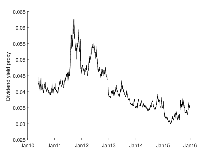
We use moments to compute the dividend and stock option prices using the maximal entropy method described in Section 3.3. We use the gradient-free Nelder-Mead simplex optimization algorithm to find the optimal parameters , and . The calibrated parameters are shown in Table 2 and the absolute pricing errors are shown in the last three columns of Table 1. The calibrated values of , , and are almost identical for different values of . This is not surprising, since these parameters mainly control the term structure of dividend futures prices, and does not enter in the pricing formula (14) for the dividend futures.22 2 Indirectly, the dividend futures prices are to some extent affected by through the inequality (11) that has to be satisfied. However, from (9) and (10) it is clear that has an impact on the volatility of the stock price and the dividend rate. Indeed, if increases, all else being equal, then the volatility of the stock price and the dividend rate increases. To offset this effect, the calibrated parameters of and are smaller for larger . From the absolute errors in Table 1, we can see that the choice of does not really matter for the quality of the calibration, since the absolute pricing errors are almost identical. The maximal relative error in the dividend futures contracts is less than , which is a remarkably good fit for a single factor model. Figure 2 visualizes the good fit of the calibrated model with the dividend futures term structure. The option prices are matched perfectly. This is a consequence of the fact that the dividend futures prices do not depend on the martingale part of and . The parameters and therefore remain free to calibrate to the dividend and stock option.
Figure 3 plots a simulation of the dividend yield process over a ten years horizon with daily discretization. We use the model parameters from Table 2 with , however the plot looks identical when using the calibrated parameters with or . The process is roughly mean-reverting around , which is the mean-reversion level of when ignoring the higher order terms in the drift. Remark that the range of values that takes in the simulation is very similar to the range of values in Figure 1.
Figure 4 shows the option price approximation as a function of the number of moments . As a benchmark, we run a Monte-Carlo simulation with daily time steps and sample paths. In order to reduce the variance of the Monte-Carlo estimator, we use a degree one polynomial in the underlying as a control variate, where we determine the coefficients of the polynomial through a least squares regression of the simulated payoff paths on the simulated polynomial. The solid line shows the Monte-Carlo estimator and the dashed lines are the corresponding confidence intervals. For the stock option, the maximal entropy approximation with four moments is already within the confidence bands and the one with six moments is exactly equal to the Monte-Carlo estimator. For the dividend option, using only two moments already provides a very accurate option price approximation. The dividend option price is easier to approximate because the volatility of the dividend rate is much lower than the volatility of the stock price.
| 0.1 | 0.0103 | -0.3440 | 0.3621 | 0.0220 | 0.0371 |
|---|---|---|---|---|---|
| 0.2 | 0.0103 | -0.3439 | 0.2813 | 0.0194 | 0.0371 |
| 0.3 | 0.0103 | -0.3439 | 0.2614 | 0.0187 | 0.0371 |


5 Extending the model with jumps
We can enrich the model dynamics by adding jumps to as follows
| (17) |
where is the same as before and is a compensated compound Poisson process with arrival intensity and with a jump distribution that is assumed to have moments in closed-form of all orders and a support . Remark that is still a continuous process, so that . Let denote a jump time of and suppose that . From the assumption on the support of , we have
where equality only holds if , in which case . Therefore, the results in Proposition 2.1 remain valid since behaves as in (2) in between jump times, we have so the process cannot jump outside of , and if so jumps to the boundary are not possible.
If we denote by the the infinitesimal generator of in the case with jumps, then we get for a twice differential function
where we assume that is such that the integral is finite and we have again omitted the function arguments for brevity, except in the first term of the integrand. Since the amplitudes of the jumps in depend linearly on and , it follows immediately that . Therefore, belongs to the class of polynomial jump-diffusions and we can compute all conditional moments in closed form.
Since enters in the dynamics of , the jumps also indirectly impact the dynamics of . The magnitude of the effect of a jump in on the drift of is determined by . A stylized fact of index options and index dividend options is that both have a negative skew in implied volatilities. Choosing a distribution with a sufficiently negative mean produces a negative skew in implied volatilities for both stock and dividend options. We leave a calibration to option skews for future work.
Remark 5.1.
It is possible to introduce jumps in as well, although one should be careful with simultaneous jumps where jumps up and jumps down in order to avoid jumping out of . We do not consider this extension in this paper.
6 Conclusion
We have introduced a model for jointly pricing stock and dividend derivatives. The novelty of our approach lies in the fact that we directly model the dividend rate while guaranteeing a positive stock price. This is accomplished by upper bounding the dividend rate by a constant fraction of the stock price, so that the dividend rate goes to zero as the stock price approaches zero. The model belongs to the class of polynomial diffusions, which leads to closed-form prices for stock and dividend futures, and efficient approximations for stock and dividend options. We have calibrated a single factor model to data on dividend futures and at-the-money stock and dividend options. Future research includes calibrating the model to stock and dividend options with a range of strikes using the extension with jumps outlined in Section 5, as well as extending our framework to discrete dividend payments.
Appendix A Proofs
A.1 Proof of Proposition 2.1
Existence of an -valued solution follows from (Ikeda and Watanabe 1981, Theorem IV.2.4), since the drift and dispersion coefficient of satisfy a linear growth condition. It remains to show that a solution starting in also stays in .
Denote by and respectively the drift and dispersion function of , i.e.
We need to verify that for with , so that the drift pushes away from the zero boundary again. Using the fact that for all , we have for all with that
The above inequality, together with , , for with , shows that for all and all . Indeed, starts in and has an inward pointing drift and vanishing diffusion at the boundary. Using the same argument for instead of , it follows that for all . As a consequence we also have .
In order to prove the non-attainment of the zero lower boundary of , we use a stochastic comparison argument. Define the process if and if . Define the process through the following SDE
From Theorem 1.3 in Hajek 1985 we get for all and
Since , we have and therefore a.s.
We use Theorem 5.7(i) in Filipović and Larsson 2016, which we restate below for completeness, to study boundary attainment of .
Theorem A.1 (Theorem 5.7(i) Filipović and Larsson 2016).
Denote by the infinitesimal generator and by the diffusion function of . Let be a polynomial and let be a vector of polynomials such that for all . If there exists a neighborhood of such that for all
| (18) |
then for all .
First, we derive conditions such that . For , we have
with the non-zero element in the -th component. For some , consider the following neighborhood of
For we have
| (19) |
If , then (19) is non-negative if . If , then we can always find an such that (19) is non-negative if .
Finally, we derive conditions such that . For we have
For some , consider the following neighborhood of
For we have
where the last line follows from . If , then on if
If , then we can always find an such that on if
For uniqueness in law of the solution , note that is an autonomous diffusion with for all . A straightforward application of Itô’s lemma shows that the process has a uniformly bounded drift and diffusion function, so that uniqueness in law for , and therefore for , follows from (Ikeda and Watanabe 1981, Theorem IV.3.3).
A.2 Proof of Proposition 2.3
To proof that is a martingale, we can use Novikov’s condition. An application of Itô’s lemma gives
which shows that is a local martingale. Since the volatility of is uniformly bounded,
Novikov’s condition is trivially satisfied and we conclude that is a martingale.
Remark A.2.
The process represents the discounted value of a trading strategy of a long position in the stock and investing all the dividends in the risk-free account. Alternatively, we could also re-invest all the dividends in the stock itself. This strategy has a discounted value process , which is again a martingale by Novikov’s condition.
Next, we show that the present value of all future dividends is equal to the stock price. Define and . The dynamics of and becomes
Taking conditional expectations and denoting and , , gives the following linear first order ODE
Using the properties of , we have that , , and for all . In particular, we have that is a non-increasing function and hence and are uniformly bounded
Moreover, all derivatives of and are uniformly bounded as well since
for all . Since is a non-increasing positive function, we have . Since is bounded, must be uniformly continuous. By Barbalat’s lemma (see e.g., Lemma 8.2 in Khalil 2002) we therefore have that . Since and , we also have componentwise. Taking the limit of gives
Since is bounded, must be uniformly continuous, and by Barbalat’s lemma we have . Since by assumption, we must have . This concludes the proof since
References
- Ackerer and Filipović (2019) Ackerer, D. and D. Filipović (2019). Linear credit risk models. Finance and Stochastics, Forthcoming.
- Baskin (1989) Baskin, J. (1989). Dividend policy and the volatility of common stocks. Journal of Portfolio Management 15(3), 19.
- Buehler (2018) Buehler, H. (2018). Volatility and dividends II: Consistent cash dividends. Available at SSRN 2639318.
- Buehler et al. (2010) Buehler, H., A. Dhouibi, and D. Sluys (2010). Stochastic proportional dividends. Working Paper.
- Filipović and Larsson (2016) Filipović, D. and M. Larsson (2016). Polynomial diffusions and applications in finance. Finance and Stochastics 20(4), 931–972.
- Filipović and Willems (2018) Filipović, D. and S. Willems (2018). A term structure model for dividends and interest rates. Swiss Finance Institute Research Paper.
- Guennoun and Henry-Labordere (2017) Guennoun, H. and P. Henry-Labordere (2017). Equity modeling with stochastic dividends. Available at SSRN 2960141.
- Hajek (1985) Hajek, B. (1985). Mean stochastic comparison of diffusions. Zeitschrift für Wahrscheinlichkeitstheorie und verwandte Gebiete 68(3), 315–329.
- Ikeda and Watanabe (1981) Ikeda, N. and S. Watanabe (1981). Stochastic Differential Equations and Diffusion Processes, Volume 24. Elsevier.
- Jaynes (1982) Jaynes, E. T. (1982). On the rationale of maximum-entropy methods. Proceedings of the IEEE 70(9), 939–952.
- Khalil (2002) Khalil, H. K. (2002). Nonlinear Systems (3rd ed.). Prentice Hall.
- Tunaru (2018) Tunaru, R. (2018). Dividend derivatives. Quantitative Finance 18(1), 63–81.