跳到论文正文
W Papers独立论文阅读器 arXiv:1908.05800 论文正文 计算阅读时间 · 0%
引用这篇论文根据当前论文元数据生成,正式投稿前建议核对。


License: arXiv.org perpetual non-exclusive license
arXiv:1908.05800v3 [math.AP] 01 Nov 2019

Orthogonality Sampling Method for the Electromagnetic Inverse Scattering Problem

Isaac Harris Thanks: Department of Mathematics, Purdue University, West Lafayette, IN 47907; (harri814@purdue.edu)    Dinh-Liem Nguyen Thanks: Department of Mathematics, Kansas State University, Manhattan, KS 66506; (dlnguyen@ksu.edu)
Abstract

This paper is concerned with the electromagnetic inverse scattering problem that aims to determine the location and shape of anisotropic scatterers from far field data (at a fixed frequency). We study the orthogonality sampling method which is a simple, fast and robust imaging method for solving the electromagnetic inverse shape problem. We first provide a theoretical foundation for the sampling method and a resolution analysis of its imaging functional. We then establish an equivalent relation between the orthogonality sampling method and direct sampling method as well as resolution analysis for the latter. The analysis uses the Factorization Method for the far field operator and it plays an important role in the justifications along with the Funk-Hecke integral identity. Finally, we present some numerical examples to validate the performance of the sampling methods for anisotropic scatterers in three dimensions.

Keywords. orthogonality sampling method, inverse electromagnetic scattering, direct sampling method, Maxwell’s equations, anisotropic media

AMS subject classification. 35R30, 35R09, 65R20

1 Introduction

In this paper, we consider the inverse shape problem that is derived from the time-harmonic electromagnetic scattering of an inhomogeneous anisotropic medium. In many physical applications such as non-destructive testing and medical imaging one wishes to infer the shape and/or material properties of the scatterer from measured electromagnetic data. We assume that the far field measurements are known and we wish to analyze two sampling methods for recovering the scatterer. Sampling methods generally fall under the category of qualitative (otherwise known as non-iterative or direct) reconstruction techniques. These methods are advantageous to use since they require little a-prior information to implement and are computationally simple. Qualitative methods have been used to solve multiple inverse shape problems in electromagnetic scattering (see for e.g. [3, 15, 10] and the references therein). These methods have also been extended to inverse problems in the time domain. In [6, 4] the linear sampling and factorization methods are extended to inverse scattering problem problems in the time domain and in [5] the MUSIC algorithm is studied for recovering small volume scatterers for the time-dependent acoustic scattering problem. Here we rigorously analyze both the orthogonality sampling method (OSM) and direct sampling method (DSM) for recovering a penetrable inhomogeneous anisotropic medium from electromagnetic far field data.

In general, sampling methods allow one to recover the scatterer by connecting the scatterer to the solution of a linear ill-posed equation involving the far field operator. Roughly speaking, the linear sampling method gives that the so-called far field equation ℱ​g=ϕ𝐲s\mathcal{F}g=\phi_{\mathbf{y}_{s}} is only solvable (via a regularization strategy) provided the sampling point is contained in the scatterer. Here the righthand side ϕ𝐲s\phi_{\mathbf{y}_{s}} is known and depends on the sampling point 𝐲s∈ℝ3\mathbf{y}_{s}\in\mathbb{R}^{3}. This allows one to define an imaging functional that is the reciprocal of the norm of the solution to the far field equation which should only be non-zero as the regularization tends to zero for sampling points in the scatterer. See [3] for the analysis of the linear sampling method for the electromagnetic scattering problem. The factorization method gives that ϕ𝐲s\phi_{\mathbf{y}_{s}} is in the range of a positive self-adjoint compact operator defined by the far field operator if and only if the sampling point is in the scatterer. By appealing to Picard’s criteria one can derive an imaging functional using the spectral decomposition of the far field operator see [15].

The OSM was first introduced in [20] for the inverse acoustic scattering from sound soft scatterers. Comparing with classical sampling methods the OSM is simpler to implement, can image (small) scatterers with only one incident field, and its stability can be easily justified. However, its mathematical foundation was only partly known. For the Helmholtz equation case, the method was rigorously justified in [20] for small scatterers and in [17] for scatterers with arbitrary shape using multi-static data. It was also first proved in [17] that the OSM is equivalent to the DSM studied in this cited paper via a remarkable connection to the analysis of the factorization method. Recently, in [11, 16] this DSM was studied in connection to the spectral decomposition of the far field operator. We also refer to [9] for the analysis of a multifrequency OSM. The OSM for Maxwell’s equations and its analysis for the case of small scatterers have been recently established in [19]. Motivated by these recent works we study in this paper the OSM for anisotropic Maxwell’s equations and provide a theoretical foundation of the method for scatterers with arbitrary shape as well as a resolution analysis for its imaging functional. Furthermore, we establish an equivalent relation between the OSM and the DSM as well as resolution analysis for the latter. The factorization analysis for the far field operator as well as the Funk-Hecke formula play an important role in our theory. We also provide numerical results for three-dimensional anisotropic scatterers to validate the efficiency of the sampling methods.

We want to mention that the DSM in [17] was extended to the electromagnetic case in [1]. This extension relies on the Factorization method analysis in [15] for an isotropic medium and the decay rate of the imaging functional was not established. Another DSM which is related to the OSM was studied in [13] for small electromagnetic scatterers. We also refer to [12, 2, 8] and references therein for results on coefficient reconstruction for the isotropic inverse electromagnetic scattering problem.

We now introduce some basic notations for the paper. Let 𝒪⊂ℝ3\mathcal{O}\subset\mathbb{R}^{3} be a domain (connected and open) with Lipschitz boundary, we indistinctly denote by (⋅,⋅)(\cdot,\cdot) the inner product of L2​(𝒪)L^{2}(\mathcal{O}) or L2​(𝒪)3L^{2}(\mathcal{O})^{3} and by ∥⋅∥\|\cdot\| the associated norms. We further denote

H⁡(curl,𝒪)\displaystyle H(\mathrm{curl}\,,\mathcal{O}) ={𝐯∈L2​(𝒪)3:curl​𝐯∈L2​(𝒪)3},\displaystyle=\big\{\mathbf{v}\in L^{2}(\mathcal{O})^{3}:\mathrm{curl}\,\mathbf{v}\in L^{2}(\mathcal{O})^{3}\big\},
Hloc​(curl,ℝ3)\displaystyle H_{\mathrm{loc}}(\mathrm{curl}\,,\mathbb{R}^{3}) ={𝐯:ℝ3→ℂ3:𝐯|B∈H(curl,B) for all ball B⊂ℝ3},\displaystyle=\big\{\mathbf{v}:\mathbb{R}^{3}\rightarrow\mathbb{C}^{3}:\mathbf{v}|_{B}\in H(\mathrm{curl}\,,B)\text{ for all ball }B\subset\mathbb{R}^{3}\big\},

where H⁡(curl,𝒪)H(\mathrm{curl}\,,\mathcal{O}) is equipped by usual inner product

(⋅,⋅)H⁡(curl,𝒪)=(curl⋅,curl⋅)+(⋅,⋅).(\cdot,\cdot)_{H(\mathrm{curl}\,,\mathcal{O})}=(\mathrm{curl}\,\cdot,\mathrm{curl}\,\cdot)+(\cdot,\cdot).

For the following sections we will first rigorously formulate the direct and inverse electromagnetic scattering problems under consideration in section 2. Section 3 is dedicated to an analysis of the far field operator and the factorization method which is necessary for the study of the OSM. We establish the main theoretical results of the paper in section 4. More precisely, we define the imaging functional for the OSM, prove its resolution and stability, and an equivalent relation to the imaging functional of the DSM. Lastly, numerical examples are given where we reconstruct bounded anisotropic scatterers in ℝ3\mathbb{R}^{3} using the electromagnetic far field data. We see that the sampling methods are robust reconstruction methods that can recover scatterers of many different shapes and sizes.

2 Direct and inverse problem formulation

We consider the scattering of time-harmonic electromagnetic waves at positive frequency ω\omega from a non-magnetic inhomogeneous medium. Suppose that there is no free charge and current density. Then, the Hloc​(curl,ℝ3)H_{\mathrm{loc}}(\mathrm{curl}\,,\mathbb{R}^{3}) electric field 𝐄{\mathbf{E}} and the magnetic field 𝐇{\mathbf{H}} satisfy the Maxwell’s equations

curl​𝐄−i​ω​μ0​𝐇=0 and curl​𝐇+i​ω​ε​𝐄=0in ​ℝ3.\displaystyle\mathrm{curl}\,{\mathbf{E}}-i\omega\mu_{0}{\mathbf{H}}=0\quad\text{ and }\quad\mathrm{curl}\,{\mathbf{H}}+i\omega\varepsilon{\mathbf{E}}=0\quad\text{in }\mathbb{R}^{3}. (1)

Here we assume that ε\varepsilon is the electric permittivity and μ0\mu_{0} (positive constant) is the magnetic permeability of the medium. The permittivity ε\varepsilon is assumed to be a bounded matrix-valued function. Let Ω\Omega be a bounded domain occupied by the non-magnetic inhomogeneous medium. The medium outside of Ω\Omega is assumed to be homogeneous. This means that there is a positive constant ε0\varepsilon_{0} such that ε=ε0​I\varepsilon=\varepsilon_{0}I outside of Ω\Omega, where II is the 3×33\times 3 identity matrix. We define the relative material parameter and the wave number as

εr=ε/ε0,k=ω​ε0​μ0.\varepsilon_{\mathrm{r}}=\varepsilon/\varepsilon_{0},\quad k=\omega\sqrt{\varepsilon_{0}\mu_{0}}.

Eliminating magnetic field 𝐇{\mathbf{H}} from (1) we obtain

curl​curl​𝐄−k2​εr​𝐄=0,in ​ℝ3.\mathrm{curl}\,\mathrm{curl}\,{\mathbf{E}}-k^{2}\varepsilon_{\mathrm{r}}{\mathbf{E}}=0,\quad\text{in }\mathbb{R}^{3}. (2)

The transmission conditions across the boundary of Ω\Omega are given by

ν×𝐄+=ν×𝐄− andν×curl​𝐄+=ν×curl​𝐄−,on ​∂Ω.\displaystyle\nu\times{\mathbf{E}}_{+}=\nu\times{\mathbf{E}}_{-}\quad\text{ and}\quad\nu\times\mathrm{curl}\,{\mathbf{E}}_{+}=\nu\times\mathrm{curl}\,{\mathbf{E}}_{-},\quad\text{on }\partial\Omega. (3)

We denote by 𝐅+\mathbf{F}_{+} and 𝐅−\mathbf{F}_{-} the traces on ∂Ω\partial\Omega from the exterior and interior of the domain Ω\Omega for a vector-valued function 𝐅\mathbf{F} respectively, and ν\nu is the unit outward normal vector on ∂Ω\partial\Omega. Assume that we illuminate the inhomogeneous anisotropic medium with the electric and magnetic incident fields 𝐄in{\mathbf{E}}_{\mathrm{in}} and 𝐇in{\mathbf{H}}_{\mathrm{in}}, respectively, satisfying

curl​𝐇in+i​ω​ε0​𝐄in=0 andcurl​𝐄in−i​ω​μ0​𝐇in=0,in ​ℝ3.\displaystyle\mathrm{curl}\,{\mathbf{H}}_{\mathrm{in}}+i\omega\varepsilon_{0}{\mathbf{E}_{\mathrm{in}}}=0\quad\text{ and}\quad\mathrm{curl}\,{\mathbf{E}_{\mathrm{in}}}-i\omega\mu_{0}{\mathbf{H}}_{\mathrm{in}}=0,\quad\text{in }\mathbb{R}^{3}.

Then there arises the scattered electric field 𝐮\mathbf{u}, defined by 𝐮:=𝐄−𝐄in\mathbf{u}:={\mathbf{E}}-{\mathbf{E}_{\mathrm{in}}}. Since the incident field 𝐄in{\mathbf{E}_{\mathrm{in}}} satisfies the homogeneous Maxwell equation with wave number kk given by

curl​curl​𝐄in−k2​𝐄in=0,in ​ℝ3\mathrm{curl}\,\mathrm{curl}\,{\mathbf{E}_{\mathrm{in}}}-k^{2}{\mathbf{E}_{\mathrm{in}}}=0,\quad\text{in }\mathbb{R}^{3}

subtracting this equation from (2) we can conclude that the scattered field 𝐮∈Hloc​(curl,ℝ3)\mathbf{u}\in H_{\mathrm{loc}}(\mathrm{curl}\,,\mathbb{R}^{3}) is the solution to

curl​curl​𝐮−k2​εr​𝐮=k2​P​𝐄inin ​ℝ3,\displaystyle\mathrm{curl}\,\mathrm{curl}\,\mathbf{u}-k^{2}\varepsilon_{\mathrm{r}}\mathbf{u}=k^{2}P{\mathbf{E}_{\mathrm{in}}}\quad\text{in }\mathbb{R}^{3}, (4)

where the contrast PP is defined by

P:=εr−I.P:=\varepsilon_{\mathrm{r}}-I.

Therefore, by definition we have that the support of the contrast PP is given by Ω\Omega. Note that we also have the corresponding transmission conditions for the scattered field 𝐮\mathbf{u} following from (3). We complete the scattering problem by the Silver-Müller radiation condition for the scattered field 𝐮\mathbf{u} given by

curl​𝐮×𝐱|𝐱|−i​k​𝐮=𝒪⁡(|𝐱|−2)as ​|𝐱|→∞,\displaystyle\mathrm{curl}\,\mathbf{u}\times\frac{\mathbf{x}}{|\mathbf{x}|}-ik\mathbf{u}=\mathcal{O}(|\mathbf{x}|^{-2})\quad\text{as }|\mathbf{x}|\rightarrow\infty, (5)

which is assumed to hold uniformly with respect to 𝐱/|𝐱|\mathbf{x}/|\mathbf{x}|.

It is known (see for e.g. [18]) that (4)–(5) is well-posed provided that the contrast PP is bounded with non-negative real and imaginary parts with support Ω\Omega provided that the only solution to the homogeneous problem (i.e. 𝐄in=0{\mathbf{E}_{\mathrm{in}}}=0) is trivial. We will assume that the homogeneous scattering problem only admits the trivial solution. This gives that the mapping 𝐄in↦𝐮{\mathbf{E}_{\mathrm{in}}}\mapsto\mathbf{u} is linear and bounded from L2​(Ω)3L^{2}(\Omega)^{3} into Hloc​(curl,ℝ3)H_{\mathrm{loc}}(\mathrm{curl}\,,\mathbb{R}^{3}).

Now we can talk about the inverse problem. To this end, we define 𝐱^=𝐱/|𝐱|\widehat{\mathbf{x}}=\mathbf{x}/|\mathbf{x}|,

𝕊2={𝐱∈ℝ3:|𝐱|=1} and Lt2(𝕊2)={𝐯∈L2(𝕊2)3:𝐱^⋅𝐯(𝐱^)=0,𝐱^∈𝕊2}.\displaystyle\mathbb{S}^{2}=\{\mathbf{x}\in\mathbb{R}^{3}:|\mathbf{x}|=1\}\quad\text{ and }\quad L^{2}_{t}(\mathbb{S}^{2})=\{\mathbf{v}\in L^{2}(\mathbb{S}^{2})^{3}:\widehat{\mathbf{x}}\cdot\mathbf{v}(\widehat{\mathbf{x}})=0,\,\,\widehat{\mathbf{x}}\in\mathbb{S}^{2}\}.

We consider the incident plane wave 𝐄in​(𝐱,𝐝,𝐪)=𝐪​ei​k​𝐱⋅𝐝{\mathbf{E}_{\mathrm{in}}}(\mathbf{x},\mathbf{d},\mathbf{q})=\mathbf{q}e^{ik\mathbf{x}\cdot\mathbf{d}}, where the vector 𝐝∈𝕊2\mathbf{d}\in\mathbb{S}^{2} indicates the direction of the incident propagation and 𝐪∈ℝ3\mathbf{q}\in\mathbb{R}^{3} is the polarization vector such that 𝐪⋅𝐝=0\mathbf{q}\cdot\mathbf{d}=0. It’s well-known that we can express the corresponding scattered wave in terms of the asymptotic expansion

𝐮⁡(𝐱,𝐝,𝐪)=ei​k​|𝐱||𝐱|​(𝐮∞​(𝐱^,𝐝,𝐪)+O⁡(1|𝐱|2)) as |𝐱|→∞,\mathbf{u}(\mathbf{x},\mathbf{d},\mathbf{q})=\frac{e^{ik|\mathbf{x}|}}{|\mathbf{x}|}\left(\mathbf{u}^{\infty}(\widehat{\mathbf{x}},\mathbf{d},\mathbf{q})+O\left(\frac{1}{|\mathbf{x}|^{2}}\right)\right)\quad\text{ as }\quad|\mathbf{x}|\to\infty,

uniformly in all observation directions 𝐱^∈𝕊2\widehat{\mathbf{x}}\in\mathbb{S}^{2}. The function 𝐮∞​(𝐱^,𝐝,𝐪)\mathbf{u}^{\infty}(\widehat{\mathbf{x}},\mathbf{d},\mathbf{q}) belonging to Lt2​(𝕊2)L_{t}^{2}(\mathbb{S}^{2}) for each incident and observation direction is called the far field pattern.

Inverse problem: Determine the shape and location of the scatterer Ω\Omega given the far field pattern 𝐮∞​(𝐱^,𝐝,𝐪)\mathbf{u}^{\infty}(\widehat{\mathbf{x}},\mathbf{d},\mathbf{q}) for all 𝐱^,𝐝∈𝕊2\widehat{\mathbf{x}},\mathbf{d}\in\mathbb{S}^{2} for a single wave number.

3 The far field operator and its factorization analysis

In this section, we will define and analyze the far field operator corresponding to (4)–(5). The analysis in this section will be used to derive sampling methods to solve the inverse shape problem of recovering the scatterer Ω\Omega from the far field data. It is well-known that the far field pattern 𝐮∞​(𝐱^,𝐝,𝐪)\mathbf{u}^{\infty}(\widehat{\mathbf{x}},\mathbf{d},\mathbf{q}) is linear in 𝐪\mathbf{q} and can be written as

𝐮∞​(𝐱^,𝐝,𝐪)=𝐮∞​(𝐱^,𝐝)​𝐪\mathbf{u}^{\infty}(\widehat{\mathbf{x}},\mathbf{d},\mathbf{q})=\mathbf{u}^{\infty}(\widehat{\mathbf{x}},\mathbf{d})\mathbf{q}

where 𝐮∞​(𝐱^,𝐝)\mathbf{u}^{\infty}(\widehat{\mathbf{x}},\mathbf{d}) is a 3×33\times 3 matrix and 𝐪⋅𝐝=0\mathbf{q}\cdot\mathbf{d}=0, see [7]. The following reciprocity relation is important in our analysis and its proof can be found in [7, Theorem 6.30].

Theorem 1.

For all 𝐱^,𝐝∈𝕊2\widehat{\mathbf{x}},\mathbf{d}\in\mathbb{S}^{2}, the far field pattern 𝐮∞​(𝐱^,𝐝)\mathbf{u}^{\infty}(\widehat{\mathbf{x}},\mathbf{d}) satisfies a reciprocity relation

𝐮∞​(𝐱^,𝐝)=[𝐮∞​(−𝐝,−𝐱^)]⊤.\mathbf{u}^{\infty}(\widehat{\mathbf{x}},\mathbf{d})=[\mathbf{u}^{\infty}(-\mathbf{d},-\widehat{\mathbf{x}})]^{\top}.

We now define the far field operator ℱ:Lt2​(𝕊2)→Lt2​(𝕊2)\mathcal{F}:L^{2}_{t}(\mathbb{S}^{2})\to L^{2}_{t}(\mathbb{S}^{2}) as

(ℱ​𝐠)​(𝐱^)=∫𝕊2𝐮∞​(𝐱^,𝐝)​𝐠​(𝐝)​𝑑s​(𝐝).(\mathcal{F}\mathbf{g})(\widehat{\mathbf{x}})=\int_{\mathbb{S}^{2}}\mathbf{u}^{\infty}(\widehat{\mathbf{x}},\mathbf{d})\mathbf{g}(\mathbf{d})\mathrm{d}s(\mathbf{d}).

In order to derive our sampling methods we will need to factorize the far field operator ℱ\mathcal{F}. To this end, it has been shown in [14] that the far field operator has the following factorization ℱ=G​H\mathcal{F}=GH. Here the operator

H:Lt2​(𝕊2)→L2​(Ω)3​ is given by ​(H​𝐠)​(𝐱)=∫𝕊2𝐠⁡(𝐝)​ei​k​𝐱⋅𝐝​𝑑s​(𝐝),𝐱∈Ω\displaystyle H:L_{t}^{2}(\mathbb{S}^{2})\to L^{2}(\Omega)^{3}\,\,\text{ is given by }\,\,(H\mathbf{g})(\mathbf{x})=\int_{\mathbb{S}^{2}}\mathbf{g}(\mathbf{d})e^{ik\mathbf{x}\cdot\mathbf{d}}\mathrm{d}s(\mathbf{d}),\quad\mathbf{x}\in\Omega (6)

and is the superposition of incident plane waves. It is easy to see that HH is compact and injective. The data to far field pattern operator

G:L2​(Ω)3→Lt2​(𝕊2) is given by G​𝐟=𝐯∞\displaystyle G:L^{2}(\Omega)^{3}\to L_{t}^{2}(\mathbb{S}^{2})\quad\text{ is given by }\quad G\mathbf{f}=\mathbf{v}^{\infty} (7)

where 𝐯∈Hloc​(curl,ℝ3)\mathbf{v}\in H_{\mathrm{loc}}(\mathrm{curl}\,,\mathbb{R}^{3}) is the solution to (4)–(5) with 𝐄in=𝐟{\mathbf{E}_{\mathrm{in}}}=\mathbf{f}. The adjoint operator H∗H^{*} of HH is given by

H∗𝐟(𝐝)=𝐝×(∫Ω𝐟(𝐱)e−ik𝐱⋅𝐝d𝐱)×𝐝,𝐝∈𝕊2.H^{*}\mathbf{f}(\mathbf{d})=\mathbf{d}\times\left(\int_{\Omega}\mathbf{f}(\mathbf{x})e^{-ik\mathbf{x}\cdot\mathbf{d}}\,\mathrm{d}\mathbf{x}\right)\times\mathbf{d},\quad\mathbf{d}\in\mathbb{S}^{2}.

From the form of the data to far field pattern operator a factorization of GG in [14] gives that G=H∗​TG=H^{*}T with

T:L2​(Ω)3→L2​(Ω)3​ is given by ​(T​𝐟)​(𝐱)=k2​P​(𝐟+𝐯)\displaystyle T:L^{2}(\Omega)^{3}\to L^{2}(\Omega)^{3}\,\,\text{ is given by }\,\,(T\mathbf{f})(\mathbf{x})=k^{2}P(\mathbf{f}+\mathbf{v}) (8)

where again 𝐯∈Hloc​(curl,ℝ3)\mathbf{v}\in H_{\mathrm{loc}}(\mathrm{curl}\,,\mathbb{R}^{3}) is the solution to (4)–(5) with 𝐄in=𝐟{\mathbf{E}_{\mathrm{in}}}=\mathbf{f}. Due to the well-posedness of the direct problem and the boundedness of PP it is clear that TT is a bounded linear operator on L2​(Ω)3L^{2}(\Omega)^{3}, and hence G=H∗​TG=H^{*}T is also a compact operator. This gives that ℱ=H∗​T​H\mathcal{F}=H^{*}TH. This factorization is used to derive the Factorization method for reconstruction Ω\Omega in [14]. In order to continue we first make the following assumptions on the domain and coefficients.

Assumption 2.

We will assume that Ω\Omega is a Lipschitz bounded domain in ℝ3\mathbb{R}^{3}. The contrast is assumed that P∈L∞​(Ω)3×3P\in L^{\infty}(\Omega)^{3\times 3}. We lastly assume that the wave number kk is not a transmission eigenvalue i.e. the only solution to the homogeneous system in L2​(Ω)3×L2​(Ω)3L^{2}(\Omega)^{3}\times L^{2}(\Omega)^{3}

curl​curl​𝐰−k2​εr​𝐰=0​ and ​curl​curl​𝝋−k2​𝝋=0 in​Ω\displaystyle\mathrm{curl}\,\mathrm{curl}\,{\bf w}-k^{2}\varepsilon_{r}{\bf w}=0\,\,\text{ and }\,\,\mathrm{curl}\,\mathrm{curl}\,\bm{\varphi}-k^{2}\bm{\varphi}=0\quad\text{ in}\,\ \Omega (9)
ν×𝐰=ν×𝝋​ and ​ν×curl​𝐰=ν×curl​𝝋on ​∂Ω\displaystyle\nu\times{\bf w}=\nu\times\bm{\varphi}\,\,\text{ and }\,\,\nu\times\mathrm{curl}\,{\bf w}=\nu\times\mathrm{curl}\,\bm{\varphi}\quad\text{on }\partial\Omega (10)

is trivial.

It is known that the set of real transmission eigenvalues is at most discrete for a real-valued permittivity and is empty for a complex-valued permittivity. See [3] and the references therein for the analysis of transmission eigenvalue problems. The following results can be found in [14]. These results will be critical in the later section where we study the orthogonality and direct sampling methods.

Theorem 3.

Let the operators HH and TT be as defined in (6)–(8) and let 𝐩,𝐲s∈ℝ3\mathbf{p},\,\mathbf{y}_{s}\in\mathbb{R}^{3}.

  1. a.

    The operator HH is compact and injective.

  2. b.

    The far field operator ℱ\mathcal{F} is compact and injective.

  3. c.

    The far field operator has the factorization ℱ=G​H\mathcal{F}=GH where G=H∗​TG=H^{*}T.

  4. d.

    Let ϕ𝐲s(𝐝)=(𝐝×𝐩)×𝐝e−ik𝐝⋅𝐲s\phi_{\mathbf{y}_{s}}(\mathbf{d})=(\mathbf{d}\times\mathbf{p})\times\mathbf{d}\,e^{-ik\mathbf{d}\cdot\mathbf{y}_{s}} then ϕ𝐲s∈Range⁡(H∗)⇔𝐲s∈Ω\phi_{\mathbf{y}_{s}}\in\mathrm{Range}(H^{*})\iff\mathbf{y}_{s}\in\Omega.

The following coercivity result from [10] is important for our theoretical analysis of the sampling methods.

Theorem 4.

Let the operator TT be as defined in (8). If the matrix-valued contrast P∈L∞​(Ω)3×3P\in L^{\infty}(\Omega)^{3\times 3} satisfies either

  1. 1.

    The imaginary part Im⁡(P)\mathrm{Im}\,(P) is uniformly positive definite or

  2. 2.

    There is a constant α≥0\alpha\geq 0 such that Re⁡(P)+α​Im​(P)\mathrm{Re}\,(P)+\alpha\mathrm{Im}\,(P) is uniformly positive definite and Im⁡(P)\mathrm{Im}\,(P) positive semidefinite.

Then provided that kk is not a transmission eigenvalue the operator TT is coercive on Range⁡(H)¯\overline{\mathrm{Range}(H)}.

Proof.

See the proof of Theorem 10 in [10] for details. ∎

4 Orthogonality sampling method

This section is dedicated to studying the OSM for solving the inverse problem. We first define the imaging functional for the OSM and then prove a resolution analysis as well as stability for the imaging functional which is the main theoretical result of this section. After that we show an equivalence between the imaging functionals of the OSM and the DSM.

The imaging functional. Let 𝐲s\mathbf{y}_{s} be the sampling points in the imaging process and 𝐩∈ℝ3\mathbf{p}\in\mathbb{R}^{3} is a fixed vector. We are interested in imaging of the scatterer Ω\Omega given the far field pattern 𝐮∞​(𝐱^,𝐝,𝐪)\mathbf{u}^{\infty}(\widehat{\mathbf{x}},\mathbf{d},\mathbf{q}), for all 𝐱^,𝐝∈𝕊2\widehat{\mathbf{x}},\mathbf{d}\in\mathbb{S}^{2} and polarization vector 𝐪=(𝐝×𝐩)×𝐝\mathbf{q}=(\mathbf{d}\times\mathbf{p})\times\mathbf{d}. We define the imaging functional ℐO​S​M\mathcal{I}_{OSM} for the OSM as

ℐO​S​M​(𝐲s):=∫𝕊2|∫𝕊2𝐮∞​(𝐱^,𝐝)​(𝐝×𝐩)×𝐝⋅(𝐱^×𝐩)×𝐱^​ei​k​𝐱^⋅𝐲s​𝑑s​(𝐱^)|2​𝑑s​(𝐝).\displaystyle\mathcal{I}_{OSM}(\mathbf{y}_{s}):=\int_{\mathbb{S}^{2}}\left|\int_{\mathbb{S}^{2}}\mathbf{u}^{\infty}(\widehat{\mathbf{x}},\mathbf{d})(\mathbf{d}\times\mathbf{p})\times\mathbf{d}\cdot(\widehat{\mathbf{x}}\times\mathbf{p})\times\widehat{\mathbf{x}}\,e^{ik\widehat{\mathbf{x}}\cdot\mathbf{y}_{s}}\mathrm{d}s(\widehat{\mathbf{x}})\right|^{2}\mathrm{d}s(\mathbf{d}). (11)

The use of (𝐝×𝐩)×𝐝(\mathbf{d}\times\mathbf{p})\times\mathbf{d} in the imaging functional is useful for the analysis in this section and to have the polarization vector belonging to Lt2​(𝕊2)L^{2}_{t}(\mathbb{S}^{2}) for any choice of 𝐩∈ℝ3\mathbf{p}\in\mathbb{R}^{3}. We now wish to write the imaging functional in terms of the far field operator. This will allow us to study the the imaging functional using the factorization analysis in the previous section.

Lemma 5.

The imaging functional ℐO​S​M\mathcal{I}_{OSM} satisfies

ℐO​S​M​(𝐲s)=‖𝐩⋅ℱ​ϕ𝐲s‖L2​(𝕊2)2,\displaystyle\mathcal{I}_{OSM}(\mathbf{y}_{s})=\|\mathbf{p}\cdot\mathcal{F}\phi_{\mathbf{y}_{s}}\|^{2}_{L^{2}(\mathbb{S}^{2})},

where ϕ𝐲s∈Lt2​(𝕊2)\phi_{\mathbf{y}_{s}}\in L^{2}_{t}(\mathbb{S}^{2}) is given by

ϕ𝐲s(𝐝)=(𝐝×𝐩)×𝐝e−ik𝐝⋅𝐲s.\displaystyle\phi_{\mathbf{y}_{s}}(\mathbf{d})=(\mathbf{d}\times\mathbf{p})\times\mathbf{d}\,e^{-ik\mathbf{d}\cdot\mathbf{y}_{s}}.
Proof.

We use the reciprocity relation and interchange the roles of 𝐱^\widehat{\mathbf{x}} and 𝐝\mathbf{d}

ℐO​S​M​(𝐲s)\displaystyle\mathcal{I}_{OSM}(\mathbf{y}_{s}) =∫𝕊2|∫𝕊2𝐮∞​(𝐱^,𝐝)​(𝐝×𝐩)×𝐝⋅(𝐱^×𝐩)×𝐱^​ei​k​𝐱^⋅𝐲s​𝑑s​(𝐱^)|2​𝑑s​(𝐝)\displaystyle=\int_{\mathbb{S}^{2}}\left|\int_{\mathbb{S}^{2}}\mathbf{u}^{\infty}(\widehat{\mathbf{x}},\mathbf{d})(\mathbf{d}\times\mathbf{p})\times\mathbf{d}\cdot(\widehat{\mathbf{x}}\times\mathbf{p})\times\widehat{\mathbf{x}}\,e^{ik\widehat{\mathbf{x}}\cdot\mathbf{y}_{s}}\mathrm{d}s(\widehat{\mathbf{x}})\right|^{2}\mathrm{d}s(\mathbf{d})
=∫𝕊2|∫𝕊2[𝐮∞​(−𝐝,−𝐱^)]⊤​(𝐝×𝐩)×𝐝⋅(𝐱^×𝐩)×𝐱^​ei​k​𝐱^⋅𝐲s​𝑑s​(𝐱^)|2​𝑑s​(𝐝)\displaystyle=\int_{\mathbb{S}^{2}}\left|\int_{\mathbb{S}^{2}}[\mathbf{u}^{\infty}(-\mathbf{d},-\widehat{\mathbf{x}})]^{\top}(\mathbf{d}\times\mathbf{p})\times\mathbf{d}\cdot(\widehat{\mathbf{x}}\times\mathbf{p})\times\widehat{\mathbf{x}}\,e^{ik\widehat{\mathbf{x}}\cdot\mathbf{y}_{s}}\,\mathrm{d}s(\widehat{\mathbf{x}})\right|^{2}\mathrm{d}s(\mathbf{d})
=∫𝕊2|∫𝕊2[𝐮∞(𝐝,𝐱^)]⊤(𝐝×𝐩)×𝐝⋅(𝐱^×𝐩)×𝐱^e−ik𝐱^⋅𝐲sds(𝐱^)|2ds(𝐝)\displaystyle=\int_{\mathbb{S}^{2}}\left|\int_{\mathbb{S}^{2}}[\mathbf{u}^{\infty}(\mathbf{d},\widehat{\mathbf{x}})]^{\top}(\mathbf{d}\times\mathbf{p})\times\mathbf{d}\cdot(\widehat{\mathbf{x}}\times\mathbf{p})\times\widehat{\mathbf{x}}\,e^{-ik\widehat{\mathbf{x}}\cdot\mathbf{y}_{s}}\,\mathrm{d}s(\widehat{\mathbf{x}})\right|^{2}\mathrm{d}s(\mathbf{d})
=∫𝕊2|∫𝕊2𝐮∞(𝐝,𝐱^)((𝐱^×𝐩)×𝐱^e−ik𝐱^⋅𝐲s)⋅(𝐝×𝐩)×𝐝ds(𝐱^)|2ds(𝐝)\displaystyle=\int_{\mathbb{S}^{2}}\left|\int_{\mathbb{S}^{2}}\mathbf{u}^{\infty}(\mathbf{d},\widehat{\mathbf{x}})((\widehat{\mathbf{x}}\times\mathbf{p})\times\widehat{\mathbf{x}}\,e^{-ik\widehat{\mathbf{x}}\cdot\mathbf{y}_{s}})\cdot(\mathbf{d}\times\mathbf{p})\times\mathbf{d}\,\mathrm{d}s(\widehat{\mathbf{x}})\right|^{2}\mathrm{d}s(\mathbf{d})
=∫𝕊2|(𝐱^×𝐩)×𝐱^⋅∫𝕊2𝐮∞(𝐱^,𝐝)(𝐝×𝐩)×𝐝e−ik𝐝⋅𝐲sds(𝐝)|2ds(𝐱^)\displaystyle=\int_{\mathbb{S}^{2}}\left|(\widehat{\mathbf{x}}\times\mathbf{p})\times\widehat{\mathbf{x}}\cdot\int_{\mathbb{S}^{2}}\mathbf{u}^{\infty}(\widehat{\mathbf{x}},\mathbf{d})({\mathbf{d}}\times\mathbf{p})\times{\mathbf{d}}\,e^{-ik{\mathbf{d}}\cdot\mathbf{y}_{s}}\,\mathrm{d}s({\mathbf{d}})\right|^{2}\mathrm{d}s(\widehat{\mathbf{x}})
=‖(𝐱^×𝐩)×𝐱^⋅ℱ​ϕ𝐲s‖L2​(𝕊2)2.\displaystyle=\left\|(\widehat{\mathbf{x}}\times\mathbf{p})\times\widehat{\mathbf{x}}\cdot\mathcal{F}\phi_{\mathbf{y}_{s}}\right\|^{2}_{L^{2}(\mathbb{S}^{2})}.

Now using the identity

(𝐱^×𝐩)×𝐱^=𝐩⁡(𝐱^⋅𝐱^)−𝐱^​(𝐱^⋅𝐩)=𝐩−𝐱^​(𝐱^⋅𝐩),(\widehat{\mathbf{x}}\times\mathbf{p})\times\widehat{\mathbf{x}}=\mathbf{p}(\widehat{\mathbf{x}}\cdot\widehat{\mathbf{x}})-\widehat{\mathbf{x}}(\widehat{\mathbf{x}}\cdot\mathbf{p})=\mathbf{p}-\widehat{\mathbf{x}}(\widehat{\mathbf{x}}\cdot\mathbf{p}),

and the fact that ℱ​ϕ𝐲s​(𝐱^)⋅𝐱^=0\mathcal{F}\phi_{\mathbf{y}_{s}}(\widehat{\mathbf{x}})\cdot\widehat{\mathbf{x}}=0, proves the claim. ∎

We have shown that the imaging functional can be represented in terms of the far field operator. We now turn our attention to studying its properties. Just as in the previous section we will assume that the contrast satisfies the assumptions of Theorem 4. This is to insure the coercivity property of the middle operator TT.

Theorem 6.

For every 𝐲s∈Ω\mathbf{y}_{s}\in\Omega the imaging functional ℐO​S​M​(𝐲s)\mathcal{I}_{OSM}(\mathbf{y}_{s}) is bounded from below by a positive constant. Moreover, for 𝐲s∉Ω\mathbf{y}_{s}\notin\Omega the imaging functional satisfies

ℐO​S​M​(𝐲s)=O⁡(1dist​(𝐲s,Ω)2),as ​dist​(𝐲s,Ω)→∞.\mathcal{I}_{OSM}(\mathbf{y}_{s})=O\left(\frac{1}{\mathrm{dist}(\mathbf{y}_{s},\Omega)^{2}}\right),\quad\text{as }\mathrm{dist}(\mathbf{y}_{s},\Omega)\to\infty.
Proof.

We first observe that using again ℱ​ϕ𝐲s​(𝐱^)⋅𝐱^=0\mathcal{F}\phi_{\mathbf{y}_{s}}(\widehat{\mathbf{x}})\cdot\widehat{\mathbf{x}}=0 and the identity (𝐱^×𝐩)×𝐱^=𝐩−𝐱^​(𝐱^⋅𝐩)(\widehat{\mathbf{x}}\times\mathbf{p})\times\widehat{\mathbf{x}}=\mathbf{p}-\widehat{\mathbf{x}}(\widehat{\mathbf{x}}\cdot\mathbf{p}) we have

⟨ℱ​ϕ𝐲s,ϕ𝐲s⟩Lt2​(𝕊2)\displaystyle\langle\mathcal{F}\phi_{\mathbf{y}_{s}},\phi_{\mathbf{y}_{s}}\rangle_{L^{2}_{t}(\mathbb{S}^{2})} =∫𝕊2ℱ​ϕ𝐲s​(𝐱^)⋅((𝐱^×𝐩)×𝐱^​ei​k​𝐱^⋅𝐲s)​𝑑s​(𝐱^)\displaystyle=\int_{\mathbb{S}^{2}}\mathcal{F}\phi_{\mathbf{y}_{s}}(\widehat{\mathbf{x}})\cdot\big((\widehat{\mathbf{x}}\times\mathbf{p})\times\widehat{\mathbf{x}}\,e^{ik\widehat{\mathbf{x}}\cdot\mathbf{y}_{s}}\big)\,\mathrm{d}s(\widehat{\mathbf{x}})
=∫𝕊2ℱ​ϕ𝐲s​(𝐱^)⋅𝐩​ei​k​𝐱^⋅𝐲s​𝑑s​(𝐱^).\displaystyle=\int_{\mathbb{S}^{2}}\mathcal{F}\phi_{\mathbf{y}_{s}}(\widehat{\mathbf{x}})\cdot\mathbf{p}\,e^{ik\widehat{\mathbf{x}}\cdot\mathbf{y}_{s}}\,\mathrm{d}s(\widehat{\mathbf{x}}).

Therefore, Lemma 5 and Cauchy-Schwarz inequality deduce that

|⟨ℱ​ϕ𝐲s,ϕ𝐲s⟩Lt2​(𝕊2)|2≤|𝕊2|2​‖𝐩⋅ℱ​ϕ𝐲s‖L2​(𝕊2)2=|𝕊2|2​ℐO​S​M​(𝐲s).\displaystyle\left|\langle\mathcal{F}\phi_{\mathbf{y}_{s}},\phi_{\mathbf{y}_{s}}\rangle_{L^{2}_{t}(\mathbb{S}^{2})}\right|^{2}\leq|\mathbb{S}^{2}|^{2}\|\mathbf{p}\cdot\mathcal{F}\phi_{\mathbf{y}_{s}}\|^{2}_{L^{2}(\mathbb{S}^{2})}=|\mathbb{S}^{2}|^{2}\mathcal{I}_{OSM}(\mathbf{y}_{s}).

Here |𝕊2||\mathbb{S}^{2}| is the surface area of 𝕊2\mathbb{S}^{2}. From the factorization ℱ=H∗​T​H\mathcal{F}=H^{*}TH and the coercive property of TT we have that

ℐO​S​M​(𝐲s)\displaystyle\mathcal{I}_{OSM}(\mathbf{y}_{s}) ≥1|𝕊2|2​|⟨H∗​T​H​ϕ𝐲s,ϕ𝐲s⟩Lt2​(𝕊2)|2\displaystyle\geq\frac{1}{|\mathbb{S}^{2}|^{2}}\left|\langle H^{*}TH\phi_{\mathbf{y}_{s}},\phi_{\mathbf{y}_{s}}\rangle_{L^{2}_{t}(\mathbb{S}^{2})}\right|^{2}
=1|𝕊2|2​|⟨T​H​ϕ𝐲s,H​ϕ𝐲s⟩Lt2​(𝕊2)|2\displaystyle=\frac{1}{|\mathbb{S}^{2}|^{2}}\left|\langle TH\phi_{\mathbf{y}_{s}},H\phi_{\mathbf{y}_{s}}\rangle_{L^{2}_{t}(\mathbb{S}^{2})}\right|^{2}
≥C​‖H​ϕ𝐲s‖4,\displaystyle\geq C\left\|H\phi_{\mathbf{y}_{s}}\right\|^{4},

where CC is some positive constant. Now let 𝐲s∈Ω\mathbf{y}_{s}\in\Omega then we have that ϕ𝐲s∈Range⁡(H∗)\phi_{\mathbf{y}_{s}}\in\mathrm{Range}(H^{*}) by Theorem 3. Therefore, we have ϕ𝐲s=H∗​φ𝐲s\phi_{\mathbf{y}_{s}}=H^{*}\varphi_{\mathbf{y}_{s}} for some φ𝐲s≠0\varphi_{\mathbf{y}_{s}}\neq 0, and

‖H​ϕ𝐲s‖\displaystyle\big\|H\phi_{\mathbf{y}_{s}}\big\| =‖H​ϕ𝐲s‖​‖φ𝐲s‖‖φ𝐲s‖\displaystyle=\frac{\big\|H\phi_{\mathbf{y}_{s}}\big\|\|\varphi_{\mathbf{y}_{s}}\|}{\|\varphi_{\mathbf{y}_{s}}\|}
≥⟨H​ϕ𝐲s,φ𝐲s⟩‖φ𝐲s‖\displaystyle\geq\frac{\langle H\phi_{\mathbf{y}_{s}},\varphi_{\mathbf{y}_{s}}\rangle}{\|\varphi_{\mathbf{y}_{s}}\|}
=⟨ϕ𝐲s,H∗​φ𝐲s⟩‖φ𝐲s‖=‖ϕ𝐲s‖2‖φ𝐲s‖>0,\displaystyle=\frac{\langle\phi_{\mathbf{y}_{s}},H^{*}\varphi_{\mathbf{y}_{s}}\rangle}{\|\varphi_{\mathbf{y}_{s}}\|}=\frac{\|\phi_{\mathbf{y}_{s}}\|^{2}}{\|\varphi_{\mathbf{y}_{s}}\|}>0,

proving the first statement of the theorem.

We now show that the imaging functional decays as dist​(𝐲s,Ω)→∞\text{dist}(\mathbf{y}_{s},\Omega)\to\infty. To do so, we first observe from Lemma 5 and the factorization ℱ=G​H\mathcal{F}=GH that

ℐO​S​M​(𝐲s)=‖𝐩⋅G​H​ϕ𝐲s‖L2​(𝕊2)2≤|𝐩|2​‖G‖2​‖H​ϕ𝐲s‖2.\mathcal{I}_{OSM}(\mathbf{y}_{s})=\|\mathbf{p}\cdot GH\phi_{\mathbf{y}_{s}}\|^{2}_{L^{2}(\mathbb{S}^{2})}\leq|\mathbf{p}|^{2}\|G\|^{2}\|H\phi_{\mathbf{y}_{s}}\|^{2}.

Therefore, we can show that ‖H​ϕ𝐲s‖2\big\|H\phi_{\mathbf{y}_{s}}\big\|^{2} satisfies the decay property and use the upper bound on the imaging functional given above. Here we let YℓmY^{m}_{\ell} denote the spherical harmonics which form a complete orthonormal system on L2​(𝕊2)L^{2}(\mathbb{S}^{2}). Now, recall the Funk-Hecke formula (see for e.g. [7])

∫𝕊2Yℓm(𝐝)e−ik𝐝⋅𝐱ds(𝐝)=4​πiℓYℓm(𝐱^)jℓ(k|𝐱|) for m∈ℕ∪{0} and ℓ=−m,…,m\int_{\mathbb{S}^{2}}Y^{m}_{\ell}(\mathbf{d})e^{-ik\mathbf{d}\cdot\mathbf{x}}\,\mathrm{d}s(\mathbf{d})=\frac{4\pi}{i^{\ell}}Y^{m}_{\ell}(\hat{\mathbf{x}})j_{\ell}(k|\mathbf{x}|)\quad\text{ for }\quad m\in\mathbb{N}\cup\{0\}\,\,\text{ and }\,\,\ell=-m,\dots,m

where jℓj_{\ell} is the first kind spherical Bessel function of order ℓ\ell. In particular,

Y00=14​π,j0​(t)=sin⁡(t)t.Y^{0}_{0}=\frac{1}{\sqrt{4\pi}},\quad j_{0}(t)=\frac{\sin(t)}{t}.

Just as in recent works [11, 19] we will use the Funk-Hecke formula to show that ‖H​ϕ𝐲s‖2\big\|H\phi_{\mathbf{y}_{s}}\big\|^{2} decays as dist​(𝐲s,Ω)→∞\text{dist}(\mathbf{y}_{s},\Omega)\to\infty. Indeed, using the Funk-Hecke formula for m=ℓ=0m=\ell=0 with the formula curl𝐳curl𝐳(𝐩e−ik𝐝⋅𝐳)=−k2(𝐝×𝐩)×𝐝e−ik𝐝⋅𝐳\mathrm{curl}\,_{\mathbf{z}}\mathrm{curl}\,_{\mathbf{z}}(\mathbf{p}e^{-ik\mathbf{d}\cdot\mathbf{z}})=-k^{2}(\mathbf{d}\times\mathbf{p})\times\mathbf{d}e^{-ik\mathbf{d}\cdot\mathbf{z}} straightforward calculations gives

∫𝕊2(𝐝×𝐩)×𝐝e−ik𝐝⋅𝐳ds(𝐝)\displaystyle\int_{\mathbb{S}^{2}}(\mathbf{d}\times\mathbf{p})\times\mathbf{d}e^{-ik\mathbf{d}\cdot\mathbf{z}}\,\mathrm{d}s(\mathbf{d}) =−1k2curl𝐳curl𝐳∫𝕊2𝐩e−ik𝐝⋅𝐳ds(𝐝)\displaystyle=-\frac{1}{k^{2}}\mathrm{curl}\,_{\mathbf{z}}\mathrm{curl}\,_{\mathbf{z}}\int_{\mathbb{S}^{2}}\mathbf{p}e^{-ik\mathbf{d}\cdot\mathbf{z}}\,\mathrm{d}s(\mathbf{d})
=−4​πk2​curl𝐳​curl𝐳​(𝐩​j0​(k​|𝐳|))=−4​πk2​(v1​(𝐳,𝐩)v2​(𝐳,𝐩)v3​(𝐳,𝐩))\displaystyle=-\frac{4\pi}{k^{2}}\mathrm{curl}\,_{\mathbf{z}}\mathrm{curl}\,_{\mathbf{z}}(\mathbf{p}j_{0}(k|\mathbf{z}|))=-\frac{4\pi}{k^{2}}\left(\begin{array}[]{ccc}v_{1}(\mathbf{z},\mathbf{p})\\ v_{2}(\mathbf{z},\mathbf{p})\\ v_{3}(\mathbf{z},\mathbf{p})\end{array}\right)

where, for j=1,2,3j=1,2,3,

vj​(𝐳,𝐩)=k2​(|𝐳|2−(𝐩⋅𝐳)​zj|𝐳|2)​j0​(k​|𝐳|)−3​((𝐩⋅𝐳)​zj|𝐳|4)​(cos⁡(k​|𝐳|)−j0​(k​|𝐳|)).\displaystyle v_{j}(\mathbf{z},\mathbf{p})=k^{2}\left(\frac{|\mathbf{z}|^{2}-(\mathbf{p}\cdot\mathbf{z})z_{j}}{|\mathbf{z}|^{2}}\right)j_{0}(k|\mathbf{z}|)-3\left(\frac{(\mathbf{p}\cdot\mathbf{z})z_{j}}{|\mathbf{z}|^{4}}\right)(\cos(k|\mathbf{z}|)-j_{0}(k|\mathbf{z}|)).

It is obvious that vj=O⁡(1/|𝐳|)v_{j}=O(1/|\mathbf{z}|) as |𝐳|→∞|\mathbf{z}|\to\infty. Therefore

(Hϕ𝐲s)(𝐱)=∫𝕊2(𝐝×𝐩)×𝐝e−ik𝐝⋅(𝐲s−𝐱)ds(𝐝)=−4​πk2(v1​(𝐲s−𝐱,𝐩)v2​(𝐲s−𝐱,𝐩)v3​(𝐲s−𝐱,𝐩))\displaystyle(H\phi_{\mathbf{y}_{s}})(\mathbf{x})=\int_{\mathbb{S}^{2}}(\mathbf{d}\times\mathbf{p})\times\mathbf{d}e^{-ik\mathbf{d}\cdot(\mathbf{y}_{s}-\mathbf{x})}\,\mathrm{d}s(\mathbf{d})=-\frac{4\pi}{k^{2}}\left(\begin{array}[]{ccc}v_{1}(\mathbf{y}_{s}-\mathbf{x},\mathbf{p})\\ v_{2}(\mathbf{y}_{s}-\mathbf{x},\mathbf{p})\\ v_{3}(\mathbf{y}_{s}-\mathbf{x},\mathbf{p})\end{array}\right)

which leads to

‖H​ϕ𝐲s‖2=O⁡(1dist​(𝐲s,Ω)2),dist​(𝐲s,Ω)→∞\|H\phi_{\mathbf{y}_{s}}\|^{2}=O\left(\frac{1}{\text{dist}(\mathbf{y}_{s},\Omega)^{2}}\right),\quad\text{dist}(\mathbf{y}_{s},\Omega)\to\infty

proving the claim. ∎

This resolution analysis implies the for any sampling points 𝐲s∈Ω\mathbf{y}_{s}\in\Omega the imaging functional is strictly positive and will decay as 𝐲s\mathbf{y}_{s} moves away from the scatterer Ω\Omega. Therefore, one can plot ℐO​S​M​(𝐲s)\mathcal{I}_{OSM}(\mathbf{y}_{s}) in order to recover the scatterer. Using the imaging functional ℐO​S​M​(𝐲s)\mathcal{I}_{OSM}(\mathbf{y}_{s}) has the advantage that one does not have to solve an ill-posed equation at each sampling point. Other sampling methods such as the Linear sampling method [3] and Factorization method [15] requires one to solve an ill-posed equation involving the far field operator at each sampling point. This requires one to compute the singular-value decomposition of the far field operator as well as applying a regularization scheme. Also stability of these methods with respect to noise added to the data is not justified where as the orthogonality sampling method only requires one to compute an inner-product and by the following theorem we see that the imaging functional is stable with respect to noise added to the far field data.

In many physical applications one only knows the far field data up to some ‘small’ perturbation. Now, assume that we only know the far field operator up to a perturbation, that means we have access to its noisy version ℱδ\mathcal{F}_{\delta}, which satisfies

‖ℱ−ℱδ‖≤δ​‖ℱ‖,\|\mathcal{F}-\mathcal{F}_{\delta}\|\leq\delta\|\mathcal{F}\|,

for some δ>0\delta>0. Here ℱδ\mathcal{F}_{\delta} represents the measured far field operator physical experiments. We now give a stablity estimate for the imaging functional ℐO​S​M​(𝐲s)\mathcal{I}_{OSM}(\mathbf{y}_{s}).

Theorem 7 (stability estimate).

Denote by ℐO​S​M,δ\mathcal{I}_{OSM,\delta} the imaging functional corresponding to noisy far field operator ℱδ\mathcal{F}_{\delta}. Then

ℐO​S​M​(𝐲s)−ℐO​S​M,δ​(𝐲s)≤|𝐩|2​|𝕊|2​‖ℱ‖2​(δ2+2​δ),for all ​𝐲s∈ℝ3,\displaystyle\mathcal{I}_{OSM}(\mathbf{y}_{s})-\mathcal{I}_{OSM,\delta}(\mathbf{y}_{s})\leq|\mathbf{p}|^{2}|\mathbb{S}|^{2}\|\mathcal{F}\|^{2}(\delta^{2}+2\delta),\quad\text{for all }\mathbf{y}_{s}\in\mathbb{R}^{3},

where |𝕊2||\mathbb{S}^{2}| is again the surface area of 𝕊2\mathbb{S}^{2}, and 𝐩∈ℝ3\mathbf{p}\in\mathbb{R}^{3} is the polarization vector in the definition of the imaging functional (11).

Proof.

Using Lemma 5, the triangle inequality and the Cauchy-Schwarz inequality we have

ℐO​S​M​(𝐲s)−ℐO​S​M,δ​(𝐲s)=‖𝐩⋅ℱ​ϕ𝐲s‖L2​(𝕊2)2−‖𝐩⋅ℱδ​ϕ𝐲s‖L2​(𝕊2)2\displaystyle\mathcal{I}_{OSM}(\mathbf{y}_{s})-\mathcal{I}_{OSM,\delta}(\mathbf{y}_{s})=\|\mathbf{p}\cdot\mathcal{F}\phi_{\mathbf{y}_{s}}\|^{2}_{L^{2}(\mathbb{S}^{2})}-\|\mathbf{p}\cdot\mathcal{F}_{\delta}\phi_{\mathbf{y}_{s}}\|^{2}_{L^{2}(\mathbb{S}^{2})}
≤‖𝐩⋅(ℱ​ϕ𝐲s−ℱδ​ϕ𝐲s)‖L2​(𝕊2)​(‖𝐩⋅ℱ​ϕ𝐲s‖L2​(𝕊2)+‖𝐩⋅ℱδ​ϕ𝐲s‖L2​(𝕊2))\displaystyle\leq\|\mathbf{p}\cdot(\mathcal{F}\phi_{\mathbf{y}_{s}}-\mathcal{F}_{\delta}\phi_{\mathbf{y}_{s}})\|_{L^{2}(\mathbb{S}^{2})}\left(\|\mathbf{p}\cdot\mathcal{F}\phi_{\mathbf{y}_{s}}\|_{L^{2}(\mathbb{S}^{2})}+\|\mathbf{p}\cdot\mathcal{F}_{\delta}\phi_{\mathbf{y}_{s}}\|_{L^{2}(\mathbb{S}^{2})}\right)
≤|𝐩|​|𝕊2|​‖ℱ−ℱδ‖​(2​‖𝐩⋅ℱ​ϕ𝐲s‖L2​(𝕊2)+‖𝐩⋅(ℱ​ϕ𝐲s−ℱδ​ϕ𝐲s)‖L2​(𝕊2))\displaystyle\leq|\mathbf{p}||\mathbb{S}^{2}|\|\mathcal{F}-\mathcal{F}_{\delta}\|\left(2\|\mathbf{p}\cdot\mathcal{F}\phi_{\mathbf{y}_{s}}\|_{L^{2}(\mathbb{S}^{2})}+\|\mathbf{p}\cdot(\mathcal{F}\phi_{\mathbf{y}_{s}}-\mathcal{F}_{\delta}\phi_{\mathbf{y}_{s}})\|_{L^{2}(\mathbb{S}^{2})}\right)
≤|𝐩|​|𝕊2||ℱ|δ⁡(2​|𝐩​‖𝕊2​|‖ℱ‖+|​𝐩‖​𝕊2|​‖ℱ‖​δ)\displaystyle\leq|\mathbf{p}||\mathbb{S}^{2}|\|\mathcal{F}\|\delta\left(2|\mathbf{p}||\mathbb{S}^{2}|\|\mathcal{F}\|+|\mathbf{p}||\mathbb{S}^{2}|\|\mathcal{F}\|\delta\right)
≤|𝐩|2​|𝕊|2​‖ℱ‖2​(δ2+2​δ),\displaystyle\leq|\mathbf{p}|^{2}|\mathbb{S}|^{2}\|\mathcal{F}\|^{2}(\delta^{2}+2\delta),

proving the theorem. ∎

Motivated by the work in [17] we prove that the imaging functionals for the OSM and DSM are equivalent. The DSM was considered in [1] for the far field operator corresponding to the magnetic field. In their analysis they assume that the contrast is scalar-valued and use the factorization established in [15]. The analysis presented here is valid for a matrix-valued contrast. Moreover, we give an explicit decay rate for the imaging function. To this end, we again let the sampling points 𝐲s\mathbf{y}_{s} and fixed vector 𝐩∈ℝ3\mathbf{p}\in\mathbb{R}^{3}, the imaging functional for the DSM is defined as

ℐD​S​M(𝐲s):=|∫𝕊2e−ik𝐝⋅𝐲s∫𝕊2𝐮∞(𝐱^,𝐝)(𝐝×𝐩)×𝐝⋅ϕ𝐲s​(𝐱^)¯ds(𝐱^)ds(𝐝)|,\displaystyle\mathcal{I}_{DSM}(\mathbf{y}_{s}):=\left|\int_{\mathbb{S}^{2}}e^{-ik\mathbf{d}\cdot\mathbf{y}_{s}}\int_{\mathbb{S}^{2}}\mathbf{u}^{\infty}(\widehat{\mathbf{x}},\mathbf{d})(\mathbf{d}\times\mathbf{p})\times\mathbf{d}\cdot\overline{\phi_{\mathbf{y}_{s}}(\widehat{\mathbf{x}})}\mathrm{d}s(\widehat{\mathbf{x}})\mathrm{d}s(\mathbf{d})\right|, (12)

where

ϕ𝐲s(𝐱^)=(𝐱^×𝐩)×𝐱^e−ik𝐱^⋅𝐲s.\phi_{\mathbf{y}_{s}}(\widehat{\mathbf{x}})=(\widehat{\mathbf{x}}\times\mathbf{p})\times\widehat{\mathbf{x}}\,e^{-ik\widehat{\mathbf{x}}\cdot\mathbf{y}_{s}}.

Now, similarly to Theorem 6 we will represent the functional in terms of the far field operator. This will be used to prove the equivalence with OSM.

Lemma 8.

The imaging functional ℐD​S​M\mathcal{I}_{DSM} for the DSM satisfies

ℐD​S​M​(𝐲s)=|⟨ℱ​ϕ𝐲s,ϕ𝐲s⟩Lt2​(𝕊2)|.\mathcal{I}_{DSM}(\mathbf{y}_{s})=\left|\langle\mathcal{F}\phi_{\mathbf{y}_{s}},\phi_{\mathbf{y}_{s}}\rangle_{L^{2}_{t}(\mathbb{S}^{2})}\right|.
Proof.

We use the reciprocity relation and interchange the roles of 𝐱^\widehat{\mathbf{x}} and 𝐝\mathbf{d}

ℐD​S​M​(𝐲s)\displaystyle\mathcal{I}_{DSM}(\mathbf{y}_{s}) =|∫𝕊2e−ik𝐝⋅𝐲s∫𝕊2[𝐮∞(−𝐝,−𝐱^)]⊤(𝐝×𝐩)×𝐝⋅(𝐱^×𝐩)×𝐱^ei​k​𝐱^⋅𝐲sds(𝐱^)ds(𝐝)|\displaystyle=\left|\int_{\mathbb{S}^{2}}e^{-ik\mathbf{d}\cdot\mathbf{y}_{s}}\int_{\mathbb{S}^{2}}[\mathbf{u}^{\infty}(-\mathbf{d},-\widehat{\mathbf{x}})]^{\top}(\mathbf{d}\times\mathbf{p})\times\mathbf{d}\cdot(\widehat{\mathbf{x}}\times\mathbf{p})\times\widehat{\mathbf{x}}\,e^{ik\widehat{\mathbf{x}}\cdot\mathbf{y}_{s}}\mathrm{d}s(\widehat{\mathbf{x}})\mathrm{d}s(\mathbf{d})\right|
=|∫𝕊2∫𝕊2𝐮∞(𝐝,𝐱^)(𝐱^×𝐩)×𝐱^e−ik𝐱^⋅𝐲s⋅(𝐝×𝐩)×𝐝ei​k​𝐝⋅𝐲sds(𝐱^)ds(𝐝)|\displaystyle=\left|\int_{\mathbb{S}^{2}}\int_{\mathbb{S}^{2}}\mathbf{u}^{\infty}(\mathbf{d},\widehat{\mathbf{x}})(\widehat{\mathbf{x}}\times\mathbf{p})\times\widehat{\mathbf{x}}\,e^{-ik\widehat{\mathbf{x}}\cdot\mathbf{y}_{s}}\cdot(\mathbf{d}\times\mathbf{p})\times\mathbf{d}\,e^{ik\mathbf{d}\cdot\mathbf{y}_{s}}\,\mathrm{d}s(\widehat{\mathbf{x}})\mathrm{d}s(\mathbf{d})\right|
=|∫𝕊2∫𝕊2𝐮∞(𝐱^,𝐝)(𝐝×𝐩)×𝐝e−ik𝐝⋅𝐲sds(𝐝)⋅(𝐱^×𝐩)×𝐱^ei​k​𝐱^⋅𝐲sds(𝐱^)|\displaystyle=\left|\int_{\mathbb{S}^{2}}\int_{\mathbb{S}^{2}}\mathbf{u}^{\infty}(\widehat{\mathbf{x}},\mathbf{d})(\mathbf{d}\times\mathbf{p})\times\mathbf{d}\,e^{-ik\mathbf{d}\cdot\mathbf{y}_{s}}\mathrm{d}s(\mathbf{d})\cdot(\widehat{\mathbf{x}}\times\mathbf{p})\times\widehat{\mathbf{x}}\,e^{ik\widehat{\mathbf{x}}\cdot\mathbf{y}_{s}}\mathrm{d}s(\widehat{\mathbf{x}})\right|
=|⟨ℱ​ϕ𝐲s,ϕ𝐲s⟩Lt2​(𝕊2)|\displaystyle=\left|\langle\mathcal{F}\phi_{\mathbf{y}_{s}},\phi_{\mathbf{y}_{s}}\rangle_{L^{2}_{t}(\mathbb{S}^{2})}\right|

proving the claim. ∎

From Theorem 6 and 8 we have all we need to derive the equivalence of the two imaging functionals studied in this section. Again we assume that the contrast satisfies the assumptions of Theorem 4. The equivalence of the two sampling methods is proven in the following result.

Theorem 9.

There exists positive constants c1c_{1} and c2c_{2} such that

c1​ℐO​S​M≤ℐD​S​M≤c2​ℐO​S​M.\displaystyle c_{1}\mathcal{I}_{OSM}\leq\mathcal{I}_{DSM}\leq c_{2}\sqrt{\mathcal{I}_{OSM}}.
Proof.

From Lemma 8, the factorization ℱ=H∗​T​H\mathcal{F}=H^{*}TH and the coercive property of TT we obtain

ℐD​S​M​(𝐲s)≥C​‖H​ϕ𝐲s‖2\mathcal{I}_{DSM}(\mathbf{y}_{s})\geq C\big\|H\phi_{\mathbf{y}_{s}}\big\|^{2}

where CC is some positive constant. The first inequality of the theorem hence follows from the estimate

ℐO​S​M​(𝐲s)=‖𝐩⋅G​H​ϕ𝐲s‖L2​(𝕊2)2≤|𝐩|2​‖G‖2​‖H​ϕ𝐲s‖2.\mathcal{I}_{OSM}(\mathbf{y}_{s})=\|\mathbf{p}\cdot GH\phi_{\mathbf{y}_{s}}\|^{2}_{L^{2}(\mathbb{S}^{2})}\leq|\mathbf{p}|^{2}\|G\|^{2}\|H\phi_{\mathbf{y}_{s}}\|^{2}.

The following estimate is from the beginning of the proof of Theorem 6

|⟨ℱ​ϕ𝐲s,ϕ𝐲s⟩Lt2​(𝕊2)|2≤|𝕊2|2​‖𝐩⋅ℱ​ϕ𝐲s‖L2​(𝕊2)2=|𝕊2|2​ℐO​S​M​(𝐲s).\displaystyle\left|\langle\mathcal{F}\phi_{\mathbf{y}_{s}},\phi_{\mathbf{y}_{s}}\rangle_{L^{2}_{t}(\mathbb{S}^{2})}\right|^{2}\leq|\mathbb{S}^{2}|^{2}\|\mathbf{p}\cdot\mathcal{F}\phi_{\mathbf{y}_{s}}\|^{2}_{L^{2}(\mathbb{S}^{2})}=|\mathbb{S}^{2}|^{2}\mathcal{I}_{OSM}(\mathbf{y}_{s}).

This estimate and Lemma 8 implies the second inequality of the theorem. ∎

Following the method for proving Theorem 6 we can obtain similar resolution analysis for the direct sampling method.

Theorem 10.

For every 𝐲s∈Ω\mathbf{y}_{s}\in\Omega the imaging functional ℐD​S​M​(𝐲s)\mathcal{I}_{DSM}(\mathbf{y}_{s}) is bounded from below by a positive constant. Moreover, for 𝐲s∉Ω\mathbf{y}_{s}\notin\Omega the imaging functional satisfies

ℐD​S​M​(𝐲s)=O⁡(1dist​(𝐲s,Ω)2),as ​dist​(𝐲s,Ω)→∞.\mathcal{I}_{DSM}(\mathbf{y}_{s})=O\left(\frac{1}{\mathrm{dist}(\mathbf{y}_{s},\Omega)^{2}}\right),\quad\text{as }\mathrm{dist}(\mathbf{y}_{s},\Omega)\to\infty.

We also have the stability of the DSM that can be proved using the triangle and the Cauchy-Schwarz inequalities. The analysis in this section allows one to solve the inverse shape problem for electromagnetic scattering by plotting either ℐD​S​M\mathcal{I}_{DSM} or ℐO​S​M\mathcal{I}_{OSM}. This amounts to a fast yet stable reconstruction method that only relies on the knowledge of the far-field data. Unlike some traditional sampling methods one does not need to minimize a non-linear functional at each sampling point.

5 Numerical examples

We present in this section several numerical examples to validate the performance of the OSM as well as the DSM. The simulations were carried on a Quad Core 3.6 GHz machine with 32GB RAM and the implementation was done using the computing software Matlab. The synthetic data are generated by numerically solving the direct problem with the spectral solver studied in [19]. We solve the direct problem (4)–(5) with incident field

𝐄in(𝐱,𝐝j,𝐪)=ik(𝐝j×𝐩)×𝐝jei​k​𝐱⋅𝐝j,j=1,2,…,N𝐝{\mathbf{E}_{\mathrm{in}}}(\mathbf{x},\mathbf{d}_{j},\mathbf{q})=ik(\mathbf{d}_{j}\times\mathbf{p})\times\mathbf{d}_{j}e^{ik\mathbf{x}\cdot\mathbf{d}_{j}},\quad j=1,2,\dots,N_{\mathbf{d}}

where 𝐩=(1/3,−1/3,1/3)⊤\mathbf{p}=(1/\sqrt{3},-1/\sqrt{3},1/\sqrt{3})^{\top} and N𝐝N_{\mathbf{d}} is the number of directions 𝐝j\mathbf{d}_{j} that is specified below for each numerical example. Likewise, we denote by N𝐱^N_{\widehat{\mathbf{x}}} the number of points 𝐱^∈𝕊2{\widehat{\mathbf{x}}}\in\mathbb{S}^{2} where the far field pattern data are collected. The points 𝐱^\widehat{\mathbf{x}} and 𝐝\mathbf{d} that are chosen for generating the scattering data are almost uniformly distributed on 𝕊2\mathbb{S}^{2}. Let

𝒟⁡(𝐱^,𝐝)=𝐮∞​(𝐱^,𝐝)​(𝐝×𝐩)×𝐝\mathcal{D}(\widehat{\mathbf{x}},\mathbf{d})=\mathbf{u}^{\infty}(\widehat{\mathbf{x}},\mathbf{d})(\mathbf{d}\times\mathbf{p})\times\mathbf{d}

be our synthetic far field data that has three components 𝒟n,n=1,2,3,\mathcal{D}_{n},n=1,2,3, and 𝒟n\mathcal{D}_{n} can be considered as an N𝐱^×N𝐝N_{\widehat{\mathbf{x}}}\times N_{\mathbf{d}} matrix. To consider noisy data, we add artificial noise to our synthetic data. More precisely, a complex-valued noise matrix 𝒩\mathcal{N} containing random numbers that are uniformly distributed in the complex square

{a+ib:|a|≤1,|b|≤1}⊂ℂ\{a+\mathrm{i}b\,:\,|a|\leq 1,\,|b|\leq 1\}\subset\mathbb{C}

is added to the data matrix 𝒟n\mathcal{D}_{n}. Denoting by δ\delta the noise level, the noisy data matrix 𝒟n,δ\mathcal{D}_{n,\delta} is then given by

𝒟n,δ:=𝒟n+δ𝒩‖𝒩‖2‖𝒟n‖2,n=1,2,3,\mathcal{D}_{n,\delta}:=\mathcal{D}_{n}+\delta\frac{\mathcal{N}}{\|\mathcal{N}\|_{2}}\left\|\mathcal{D}_{n}\right\|_{2},\quad n=1,2,3,

where ∥⋅∥2\|\cdot\|_{2} is the matrix 2-norm. To define the anisotropic contrasts for the numerical examples, we need the following diagonal matrix

A=[10001.50001.2].\displaystyle A=\left[\begin{array}[]{ccccc}1&0&0\\ 0&1.5&0\\ 0&0&1.2\end{array}\right].

5.1 OSM and DSM (Figure 1).

We present in Figure 1 the reconstruction results of the OSM and DSM for an anisotropic scatterer including three different balls. The scatterer is characterized by smoothly varying contrast P⁡(𝐱)P(\mathbf{x}) defined by

Ω1\displaystyle\Omega_{1} ={𝐱∈ℝ3:|𝐱−𝐚|2<0.32,𝐚=(0.4,0,−0.45)⊤}\displaystyle=\left\{\mathbf{x}\in\mathbb{R}^{3}:|\mathbf{x}-\mathbf{a}|^{2}<0.3^{2},\mathbf{a}=(0.4,0,-0.45)^{\top}\right\}
Ω2\displaystyle\Omega_{2} ={𝐱∈ℝ3:|𝐱−𝐛|2<0.352,𝐛=(−0.4,0,0)⊤}\displaystyle=\left\{\mathbf{x}\in\mathbb{R}^{3}:|\mathbf{x}-\mathbf{b}|^{2}<0.35^{2},\mathbf{b}=(-0.4,0,0)^{\top}\right\}
Ω3\displaystyle\Omega_{3} ={𝐱∈ℝ3:|𝐱−𝐜|2<0.42,𝐜=(0.4,0,0.4)⊤}\displaystyle=\left\{\mathbf{x}\in\mathbb{R}^{3}:|\mathbf{x}-\mathbf{c}|^{2}<0.4^{2},\mathbf{c}=(0.4,0,0.4)^{\top}\right\}
P⁡(𝐱)\displaystyle P(\mathbf{x}) ={Aexp(1−0.320.32−|𝐱−𝐚|2),𝐱∈Ω1Aexp(1−0.3520.352−|𝐱−𝐛|2),𝐱∈Ω2Aexp(1−0.420.42−|𝐱−𝐜|2),𝐱∈Ω30,else,\displaystyle=\begin{cases}A\exp\left(1-\frac{0.3^{2}}{0.3^{2}-|\mathbf{x}-\mathbf{a}|^{2}}\right),\quad&\mathbf{x}\in\Omega_{1}\\ A\exp\left(1-\frac{0.35^{2}}{0.35^{2}-|\mathbf{x}-\mathbf{b}|^{2}}\right),\quad&\mathbf{x}\in\Omega_{2}\\ A\exp\left(1-\frac{0.4^{2}}{0.4^{2}-|\mathbf{x}-\mathbf{c}|^{2}}\right),\quad&\mathbf{x}\in\Omega_{3}\\ 0,\quad&\text{else},\end{cases} (16)

where AA is given by (5).

Here we choose wave number k=12k=12 (the corresponding wavelength is about 0.52) and N𝐱^×N𝐝=325×325N_{\widehat{\mathbf{x}}}\times N_{\mathbf{d}}=325\times 325. The far field data are perturbed by 30%\% noise. In Figure 1 we also present 3D-visualizations of the exact geometry and its reconstructions using isosurface in Matlab. The isovalue for the isosurface plotting is chosen to be 1/31/3 of the maximal value of the computed imaging functionals ℐO​S​M\mathcal{I}_{OSM} and ℐD​S​M\mathcal{I}_{DSM}. It can be seen in Figure 1 that both the OSM and the DSM are robust with noise added to the data and provide reasonable reconstructions of the scatterer. We also observe that the reconstruction from ℐO​S​M\mathcal{I}_{OSM} is more similar to that from (ℐD​S​M)2(\mathcal{I}_{DSM})^{2} rather than the one from ℐD​S​M\mathcal{I}_{DSM}. This might reflect the estimate ℐD​S​M≤c2​ℐO​S​M\mathcal{I}_{DSM}\leq c_{2}\sqrt{\mathcal{I}_{OSM}} from the equivalent relation in Theorem 9.

Refer to caption
(a)
Refer to caption
(b)
Refer to caption
(c)
Refer to caption
(d)
Refer to caption
(e)
Refer to caption
(f)
Refer to caption
(g)
Refer to caption
(h)
Figure 1: Reconstruction with OSM and DSM for the scatterer including three different balls. N𝐱^×N𝐝=325×325N_{\widehat{\mathbf{x}}}\times N_{\mathbf{d}}=325\times 325, wave number k=12k=12. There is 30%\% noise added to the data. (a) Exact geometry. (b) Reconstruction with ℐO​S​M\mathcal{I}_{OSM}. (c) Reconstruction with ℐD​S​M\mathcal{I}_{DSM}. (d) Reconstruction with (ℐD​S​M)2(\mathcal{I}_{DSM})^{2}. (e) Cross-sectional view of the exact geometry. (f) Cross-sectional view of the computed ℐO​S​M\mathcal{I}_{OSM}. (g) Cross-sectional view of the computed ℐD​S​M\mathcal{I}_{DSM}. (h) Cross-sectional view of the computed (ℐD​S​M)2(\mathcal{I}_{DSM})^{2}. The isovalue in the isosurface plotting is 1/31/3 of the maximal value of the computed imaging functionals.

5.2 OSM for highly noisy data (Figure 2).

The second example is presented in Figure 2 where we focus on performance of the sampling method on data perturbed by high amounts of noise.

Here consider the scatterer as in the previous example (16), k=12k=12 and N𝐱^×N𝐝=325×325N_{\widehat{\mathbf{x}}}\times N_{\mathbf{d}}=325\times 325. From Figure 2 we can see that, even there are high levels of noise δ=0.6\delta=0.6 and 0.90.9 in the far field data, that the OSM is still able to provide reasonable reconstructions. The computed images are not very different for 60%\% and 90%\% noise in the data. The solid performance of the method on noisy data can be justified by the stability of the method that is discussed in Theorem 7.

Refer to caption
(a)
Refer to caption
(b)
Refer to caption
(c)
Refer to caption
(d)
Refer to caption
(e)
Refer to caption
(f)
Figure 2: Reconstruction with highly noisy data using OSM. N𝐱^×N𝐝=325×325N_{\widehat{\mathbf{x}}}\times N_{\mathbf{d}}=325\times 325, wave number k=12k=12. (a) Exact geometry. (b) Reconstruction for 60%\% noise. (c) Reconstruction for 90%\% noise. (d) Cross-sectional view of the exact geometry. (e) Cross-sectional view of the computed ℐO​S​M\mathcal{I}_{OSM} for 60%\% noise. (f) Cross-sectional view of the computed ℐO​S​M\mathcal{I}_{OSM} for 90%\% noise. The isovalue in the isosurface plotting is 1/31/3 of the maximal value of the computed ℐO​S​M\mathcal{I}_{OSM}.

5.3 OSM with less data (Figure 3).

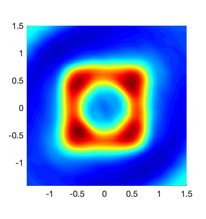
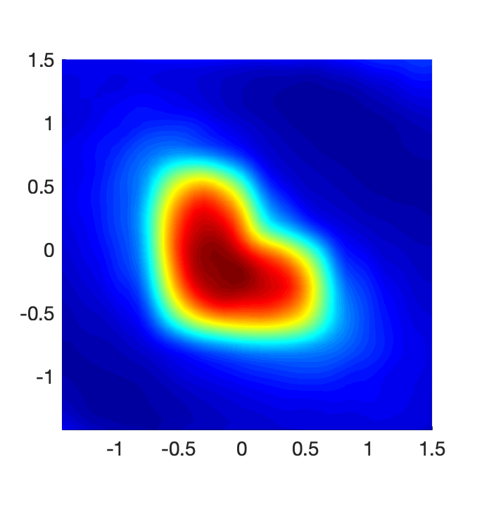
This is the focus of the third example that is to examine the performance of the OSM on a smaller wave number and a smaller set of scattering data. We consider the same scatterer as in the first and second examples (16). The data in this example are perturbed by 30%\% noise. We can see in Figure 3(b) that for N𝐱^×N𝐝=325×325N_{\widehat{\mathbf{x}}}\times N_{\mathbf{d}}=325\times 325 and wave number k=6k=6 (wavelength is about 1.04) the reconstruction is not as good as that of the case k=12k=12 (Figure 3(c)). Although we can see two components of the scatterers in the reconstruction the shape and locations are not very accurate. The result is even worse if we have less data, see Figure 3(d). More precisely, for N𝐱^×N𝐝=91×91N_{\widehat{\mathbf{x}}}\times N_{\mathbf{d}}=91\times 91 and k=12k=12, the reconstruction is no longer reasonable.

Refer to caption
(a)
Refer to caption
(b)
Refer to caption
(c)
Refer to caption
(d)
Figure 3: Reconstruction with a smaller wave number and a smaller amount of scattering data in cross-sectional views of the computed ℐO​S​M\mathcal{I}_{OSM}. There is 30%\% noise added to the data. (a) Exact geometry. (b) N𝐱^×N𝐝=325×325N_{\widehat{\mathbf{x}}}\times N_{\mathbf{d}}=325\times 325 and k=6k=6. (c) N𝐱^×N𝐝=325×325N_{\widehat{\mathbf{x}}}\times N_{\mathbf{d}}=325\times 325 and k=12k=12. (d) N𝐱^×N𝐝=91×91N_{\widehat{\mathbf{x}}}\times N_{\mathbf{d}}=91\times 91 and k=12k=12.

5.4 OSM for other types of scatterers (Figure 4).

In this example we present in Figure 4 the reconstruction results for three different types of scatterers. We consider scatterers with more complicated shapes and non-smooth geometries. For the scatterer in Figure 4(a) the anisotropic contrast P⁡(𝐱)P(\mathbf{x}) is again a smoothly varying function defined by

D1\displaystyle D_{1} ={𝐱∈ℝ3:|𝐱−𝐚|2<0.32,𝐚=(0,0,0.4)⊤}\displaystyle=\left\{\mathbf{x}\in\mathbb{R}^{3}:|\mathbf{x}-\mathbf{a}|^{2}<0.3^{2},\mathbf{a}=(0,0,0.4)^{\top}\right\}
D2\displaystyle D_{2} ={𝐱∈ℝ3:|𝐱−𝐛|2<0.52,𝐛=(0,0,−0.3)⊤}\displaystyle=\left\{\mathbf{x}\in\mathbb{R}^{3}:|\mathbf{x}-\mathbf{b}|^{2}<0.5^{2},\mathbf{b}=(0,0,-0.3)^{\top}\right\}
P⁡(𝐱)\displaystyle P(\mathbf{x}) ={A2exp(1−0.320.32−|𝐱−𝐚|2),𝐱∈D1A2exp(1−0.520.52−|𝐱−𝐛|2),𝐱∈D20,else,\displaystyle=\begin{cases}\frac{A}{2}\exp\left(1-\frac{0.3^{2}}{0.3^{2}-|\mathbf{x}-\mathbf{a}|^{2}}\right),\quad&\mathbf{x}\in D_{1}\\ \frac{A}{2}\exp\left(1-\frac{0.5^{2}}{0.5^{2}-|\mathbf{x}-\mathbf{b}|^{2}}\right),\quad&\mathbf{x}\in D_{2}\\ 0,\quad&\text{else},\end{cases}

where matrix AA is given by (5). The contrast P⁡(𝐱)P(\mathbf{x}) for the scatterers in Figures 4(d) and 4(g) are respectively equal to A/2A/2 and A/4A/4 in Ω\Omega and 0 outside of Ω\Omega. Again, N𝐱^×N𝐝=325×325N_{\widehat{\mathbf{x}}}\times N_{\mathbf{d}}=325\times 325, k=12k=12 and the data are perturbed by 30%\% noise. The pictures show that with the right amount of data the sampling method is able to provide good reconstruction results for scatterers with more complicated shapes. We also observe that for scatterers with non-smooth geometries like in Figures 4(d) and 4(g), the isovalue in the isosurface plotting should be 1/2 of the maximal value of the computed imaging functional ℐO​S​M\mathcal{I}_{OSM} to give a better three-dimensional image.

Refer to caption
(a)
Refer to caption
(b)
Refer to caption
(c)
Refer to caption
(d)
Refer to caption
(e)
Refer to caption
(f)
Refer to caption
(g)
Refer to caption
(h)
Refer to caption
(i)
Figure 4: Reconstruction of scatterers with more complicated shapes using OSM. There is 30%\% noise in the scattering data, N𝐱^×N𝐝=325×325N_{\widehat{\mathbf{x}}}\times N_{\mathbf{d}}=325\times 325 and k=12k=12. The first column is the exact geometries and the second column is the corresponding reconstructions. Cross-sectional views of the computed ℐO​S​M\mathcal{I}_{OSM} are displayed in the last column. The isovalues in the isosurface plotting are respectively 1/31/3 and 1/21/2 of the maximal value of the computed ℐO​S​M\mathcal{I}_{OSM} for (b) and (e, h).

6 Summary

We study the OSM for solving the electromagnetic inverse scattering problem for anisotropic media with far field data. We propose an imaging functional for the OSM which is able to compute the location and shape of electromagnetic scatterers in a fast and robust way. Using tools of the Factorization method analysis and the Funk-Hecke formula we are able to establish a rigorous justification and resolution analysis for the proposed imaging functional. We also prove that this functional is equivalent to that of the DSM and that our resolution analysis for the OSM can be directly applied to the DSM. Numerical results for three-dimensional anisotropic scatterers are presented. Together with our recent work in [19], where the OSM is justified for the electromagnetic inverse scattering with one incident plane wave, we have provided a versatile approach for solving the electromagnetic inverse scattering problem.

Acknowledgement. The work of DLN is partially supported by NSF grant DMS-1812693.

References

  • [1] A.-M. Alzaalig. Direct Sampling Methods for Inverse Scattering Problems. PhD thesis, Michigan Technological University, 2017.
  • [2] G. Bao and P. Li. Numerical solution of an inverse medium scattering problem for maxwell’s equations at fixed frequency. J. Comput. Phys., 228:4638–4648, 2009.
  • [3] F. Cakoni, D. Colton, and P. Monk. The Linear Sampling Method in Inverse Electromagnetic Scattering. SIAM, 2011.
  • [4] F. Cakoni, H. Haddar, and A. Lechleiter. On the factorization method for a far field inverse scattering in the time domain. SIAM J. Math. Anal., 51:854–872, 2019.
  • [5] F. Cakoni and J. Rezac. Direct imaging of small scatterers using reduced time dependent data. J. Comput. Phys., 338:371–387, 2017.
  • [6] Q. Chen, H. Haddar, A. Lechleiter, and P. Monk. A sampling method for inverse scattering in the time domain. Inverse Problems, 26:085001, 2010.
  • [7] D. Colton and R. Kress. Inverse Acoustic and Electromagnetic Scattering Theory. Springer, New York, 3rd edition, 2013.
  • [8] M. de Buhan and M. Darbas. Numerical resolution of an electromagnetic inverse medium problem at fixed frequency. Comput. Math. Appl., 74:3111–3128, 2017.
  • [9] R. Griesmaier. Multi-frequency orthogonality sampling for inverse obstacle scattering problems. Inverse Problems, 27:085005, 2008.
  • [10] H. Haddar. Analysis of some qualitative methods for inverse electromagnetic scattering problems. In Bermudez de Castro A., Valli A. (eds) Computational Electromagnetism. Lecture Notes in Mathematics, vol 2148, pages 191–240. Springer, Cham, 2014.
  • [11] I. Harris and A. Kleefeld. Analysis of new direct sampling indicators for far-field measurements. Inverse Problems, 35:054002, 2019.
  • [12] T. Hohage. On the numerical solution of a three-dimensional inverse medium scattering problem. Inverse Problems, 17:1743–1763, 2001.
  • [13] K. Ito, B. Jin, and J. Zou. A direct sampling method for inverse electromagnetic medium scattering. Inverse Problems, 29:095018, 2013.
  • [14] A. Kirsch. The factorization method for Maxwell’s equations. Inverse Problems, 20:S117–S134, 2004.
  • [15] A. Kirsch and N.I. Grinberg. The Factorization Method for Inverse Problems. Oxford Lecture Series in Mathematics and its Applications 36. Oxford University Press, 2008.
  • [16] K. H. Leem, J. Liu, and G. Pelekanos. Two direct factorization methods for inverse scattering problems. Inverse Problems, 34:125004, 2018.
  • [17] X. Liu. A novel sampling method for multiple multiscale targets from scattering amplitudes at a fixed frequency. Inverse Problems, 33:085011, 2017.
  • [18] P. Monk. Finite Element Methods for Maxwell’s Equations. Oxford Science Publications, Oxford, 2003.
  • [19] D.-L. Nguyen. Direct and inverse electromagnetic scattering problems for bi-anisotropic media. Inverse Problems (accepted), https://doi.org/10.1088/1361-6420/ab382d.
  • [20] R. Potthast. A study on orthogonality sampling. Inverse Problems, 26:074015, 2010.