跳到论文正文
W Papers独立论文阅读器 arXiv:1908.05719 论文正文 计算阅读时间 · 0%
引用这篇论文根据当前论文元数据生成,正式投稿前建议核对。


License: arXiv.org perpetual non-exclusive license
arXiv:1908.05719v2 [math.AP] 03 Feb 2020

On a Fractional Schrödinger equation in the presence of Harmonic potential

Zhiyan Ding Note: Department of Mathematics, University of Wisconsin, Madison (zding49@wisc.edu)    Hichem Hajaiej Note: California State University, Los angeles, 5151 University Drive (hhajaie@calstatela.edu)
Abstract

In this paper, we establish the existence of ground state solutions for a fractional Schrödinger equation in the presence of a harmonic trapping potential. We also address the orbital stability of standing waves. Additionally, we provide interesting numerical results about the dynamics and compare them with other types of Schrödinger equations [9, 15]. Our results explain the effect of each term of the Schrödinger equation : The fractional power, the power of the nonlinearity and the harmonic potential.

Keywords: Schrödinger equation, fractional Laplacian, harmonic potential, standing waves

MSC 2010: 35Q55, 35J60, 47J30

1 Fractional Nonlinear Schrödinger equation with harmonic potential

In this paper, we examine the following Schrödinger equation:

{i​ψt=(−Δ)s​ψ+|x|2​ψ−|ψ|2​σ​ψ​in​ℝN×[0,∞),ψ⁡(0,x)=ψ0​(x)∈Hs​(ℝN),\left\{\begin{aligned} &i\psi_{t}=(-\Delta)^{s}\psi+|x|^{2}\psi-|\psi|^{2\sigma}\psi\;\;\mbox{in}\;\mathbb{R}^{N}\times[0,\infty),\\ &\psi(0,x)=\psi_{0}(x)\in H_{s}(\mathbb{R}^{N}),\end{aligned}\right. (1)

where 0<s<10<s<1, σ>0\sigma>0, N≥1N\geq 1 and ψ:ℝN×[0,∞)⟶ℂ\psi:\mathbb{R}^{N}\times[0,\infty)\longrightarrow\mathbb{C} is the wave function with initial condition ψ0​(x)\psi_{0}(x) belongs to the following Sobolev space:

Hs​(ℝN):={u∈L2​(ℝN):∫ℝN∫ℝN|u⁡(x)−u⁡(y)|2|x−y|N+2​s​𝑑y​𝑑x<∞}.H_{s}(\mathbb{R}^{N}):=\left\{u\in L^{2}(\mathbb{R}^{N}):\int_{\mathbb{R}^{N}}\int_{\mathbb{R}^{N}}\frac{|u(x)-u(y)|^{2}}{|x-y|^{N+2s}}dydx<\infty\right\}.

with

‖u‖Hs​(ℝN)=∫ℝN∫ℝN|u⁡(x)−u⁡(y)|2|x−y|N+2​s​𝑑y​𝑑x+∫ℝN|u⁡(x)|2​𝑑x\|u\|_{H_{s}(\mathbb{R}^{N})}=\sqrt{\int_{\mathbb{R}^{N}}\int_{\mathbb{R}^{N}}\frac{|u(x)-u(y)|^{2}}{|x-y|^{N+2s}}dydx+\int_{\mathbb{R}^{N}}|u(x)|^{2}dx}

The fractional Laplacian (−Δ)s(-\Delta)^{s} is defined via a pseudo-differential operator

(−Δ)s​u​(x)=ℱ−1​[|ξ|2​s​[u]],s>0.(-\Delta)^{s}u(x)=\mathcal{F}^{-1}[|\xi|^{2s}\mathcal{[}u]],\ s>0. (2)

For the Cauchy problem (1), we have two important conserved quantities: The mass of the wave function:

M⁡(t)=‖ψ⁡(⋅,t)‖2:=∫ℝN|ψ⁡(x,t)|2​𝑑x≡M⁡(0)M(t)=||\psi(\cdot,t)||^{2}:=\int_{\mathbb{R}^{N}}|\psi(x,t)|^{2}dx\equiv M(0) (3)

and the total energy:

E⁡(t)=∫ℝN[Re​(ψ∗​(x,t)​(−Δ)s​ψ)+|x|2​|ψ|2−1σ+1​|ψ⁡(x,t)|2​(σ+1)]​𝑑x≡E⁡(0).E(t)=\int_{\mathbb{R}^{N}}\left[\text{Re}\left(\psi^{*}(x,t)(-\Delta)^{s}\psi\right)+|x|^{2}|\psi|^{2}-\frac{1}{\sigma+1}|\psi(x,t)|^{2(\sigma+1)}\right]dx\equiv E(0). (4)

In recent years, a great attention has been focused on the study of problems involving the fractional Laplacian, which naturally appears in obstacle problems, phase transition, conservation laws, financial market. Nonlinear fractional Schrödinger equations have been proposed by Laskin [16, 17] in order to expand the Feynman path integral, from the Brownian like to the Lévy like quantum mechanical paths. The stationary solutions of fractional nonlinear Schrödinger equations have also been intensively studied due to their huge importance in nonlinear optics and quantum mechanics [16, 17, 12, 10]. The most interesting solutions have the special form:

ψ⁡(x,t)=e−i​λ​t​u​(x),λ∈ℝ,u⁡(x)∈ℂ.\psi(x,t)=e^{-i\lambda t}u(x),\;\;\lambda\in\mathbb{R},\;\;u(x)\in\mathbb{C}. (5)

They are called the standing waves. These solutions reduce (1) to a semilinear elliptic equation. In fact, after plugging (5) into (1), we need to solve the following equation

(−Δ)s​u​(x)+|x|2​u​(x)−|u⁡(x)|2​σ​u​(x)=λ​u​(x)​in​ℝN×[0,∞).(-\Delta)^{s}u(x)+|x|^{2}u(x)-|u(x)|^{2\sigma}u(x)=\lambda u(x)\;\;\mbox{in}\;\mathbb{R}^{N}\times[0,\infty). (6)

The case s=1s=1 has been intensively studied by many authors (See [20]). There also exist a considerable amount of results concerning the standing waves of fractional Nonlinear Schrödinger equations without the harmonic potential, we refer the readers to [3, 6, 5, 8, 11, 13, 18, 19] and the references therein.

In this paper, we mainly focus on the solutions to (6). To the best of our knowledge, our results are new and will open the way to solve other class of fractional Schrödinger equations. This paper has two main parts: In the first part, we address the existence of standing waves through a particular variational form, whose solutions are called ground state solutions. We prove the existence of ground state solutions (Theorem 2.1), and show some qualitative properties like monotonicity and radiality (Lemma 3.2). We also proved that the ground state solutions are orbitally stable (Def 4.1, Theorem 2.2) if we have the uniqueness of the solutions for the Cauchy problem (1) (Theorem 4.1). We have also addressed the critical case σ=2​sN\sigma=\frac{2s}{N}, which is consistent with the case s=1s=1 in [9]. The second part of this article deals with the numerical method to solve (1) and to establish the existence of ground state solutions as well as to establish the optimality of our conditions. In this part, we were not only able to show the existence of ground state solutions for 0<σ<2​sN0<\sigma<\frac{2s}{N} but we also gave a constrained variational problem ((62)-(63)), which was crucial to find the standing waves for the subcritical 2​sN≤σ<2​sN−2​s\frac{2s}{N}\leq\sigma<\frac{2s}{N-2s}. The numerical results provided a good explanation of the effect of ss on the ground state solution. To reach this goal, we showed the ground state solution is continuous and decreasing with respect to ss in L2L^{2} and L∞L^{\infty} norm (Figure 2), which is a similar phenomenon to [15]. Besides, like Gross–Pitaevskii Equation [9], we examined the convergence property of λc\lambda_{c}. It turned out this convergence property also holds true in our case. Second, we checked the stability of ground state solutions for different ss. If we add a small perturbation to the initial condition, for different ss, the absolute value of the solution will always have periodic behavior, which shows the orbital stability (Figure 6). Furthermore, surprisingly, when ss becomes smaller, the stability is worse, which means the oscillation amplitude in the periodic phenomenon becomes larger (Figure 8,9(a)). We then address the case where the harmonic potential is not radial, and we obtained non radial symmetrical ground state solution (Figure 5(a),5(b)). Finally, we provided interesting numerical results for the time dynamics of FNLS.

The main difficulty of constructing ground state solutions comes from the lack of compactness of the Sobolev embeddings for the unbounded domain ℝN\mathbb{R}^{N}. However, by defining an appropriate function space, in which the norm of the potential is involved, we ”recuperate” the compactness (see Lemma 3.1). This fact, combined with rearrangement inequalities are the key points to prove the existence of ground state solutions. In the numerical part, the presence of the harmonic potential term is challenging. In fact, one can’t take Fourier transfrom directly on both sides of the equation like [15] because we have nonlinear term. Different from [9], we also can’t use finite difference directly since fractional Laplacian is not a local term. Consequtently, we opted idea from [7] and use time splitting method. By our splitting, we can obtain specific solutions in each small step and also preserve the mass (3). For the ground state solutions, the classical Newton’s method [9] is too slow because we have to deal with fractional Laplacian. To overcome this, we borrow idea from [2] and use normalized gradient flow (NGF) to find the ground state solutions. Moreover, for the case 2​sN≤σ≤2​sN−2​s\frac{2s}{N}\leq\sigma\leq\frac{2s}{N-2s}, we have noticed that the energy in the original variational problem can not be bounded from below, therefore, we present a new constrained variational problem ((62)-(63)) to establish the existence of ground state solutions.

The paper is organized as follows. In section 2, we give our main results about the existence of ground state solutions and orbital stability of standing waves. In section 3, we provide the proof of the existence. Then, in section 4, we discuss the orbital stability. In section 5, we use Split-Step Fourier Spectral method to solve (1) numerically. In section 6, instead of using common iterative Newton’s method, we use the NGF method to find ground states when 0<σ≤2​sN−2​s0<\sigma\leq\frac{2s}{N-2s}. Finally, in section 7, we present our numerical results for the dynamics (1) and compare them with other kinds of Schrödinger equations ([9, 15]).

2 Main results

We use a variational formulation to examine the solution to (6). First, note that if λ=0\lambda=0, we can find solutions u⁡(x)u(x) to (6) from the critical points of the functional 𝒥:Hs​(ℝN)⟶ℝ\mathcal{J}:H_{s}(\mathbb{R}^{N})\longrightarrow\mathbb{R} defined as:

𝒥⁡(u)=12​‖∇su‖22+12​∫ℝN|x|2​|u|2​𝑑x−12​σ+2​∫ℝN|u|2​σ+2​𝑑x,\mathcal{J}(u)=\frac{1}{2}\|\nabla_{s}u\|_{2}^{2}+\frac{1}{2}\int_{\mathbb{R}^{N}}|x|^{2}|u|^{2}dx-\frac{1}{2\sigma+2}\int_{\mathbb{R}^{N}}|u|^{2\sigma+2}dx, (7)

where ∥.∥L2\|.\|_{L^{2}} is the L2L^{2}-norm and ‖∇su‖2\|\nabla_{s}u\|_{2} is defined by

‖∇su‖22=CN,s​∫ℝN∫ℝN|u⁡(x)−u⁡(y)|2|x−y|N+2​s​𝑑x​𝑑y,\|\nabla_{s}u\|_{2}^{2}=C_{N,s}\int_{\mathbb{R}^{N}}\int_{\mathbb{R}^{N}}\frac{|u(x)-u(y)|^{2}}{|x-y|^{N+2s}}dxdy,

with some normalization constant CN,sC_{N,s}.

We can derive (7) by multiplying smooth enough test function v⁡(x)v(x) on both sides of (6) and taking the integral over xx. However, instead of directly finding the critical points of (7), we consider a reconstructed variational problem, which can help us to find solutions with different λ\lambda and any energy. Specifically, for a fixed number c>0c>0, we need to solve the following constrained minimization problem.

Ic=i​n​f​{𝒥⁡(u):u∈Sc},I_{c}=inf\left\{\mathcal{J}(u):u\in S_{c}\right\}, (8)

with

Sc={u∈Σs​(ℝN):∫ℝN|u|2​𝑑x=c2},S_{c}=\left\{u\in\Sigma_{s}(\mathbb{R}^{N}):\int_{\mathbb{R}^{N}}|u|^{2}dx=c^{2}\right\}, (9)

where

Σs​(ℝN)={u∈Hs​(ℝN):‖u‖Σs​(ℝN):=‖u‖L2​(ℝN)+‖∇su‖L2​(ℝN)+‖x​u‖L2​(ℝN)<∞}.\Sigma_{s}({\mathbb{R}^{N}})=\left\{u\in H_{s}(\mathbb{R}^{N}):\|u\|_{\Sigma_{s}({\mathbb{R}^{N}})}:=\|u\|_{L^{2}({\mathbb{R}^{N}})}+\|\nabla_{s}u\|_{L^{2}({\mathbb{R}^{N}})}+\|xu\|_{L^{2}({\mathbb{R}^{N}})}<\infty\right\}. (10)

is a Hilbert space, with corresponding natural inner product.

We claim that for each minimizer u⁡(x)u(x) of the constrained minimization problem (8), there exists some λ\lambda such that (u⁡(x),λ)(u(x),\lambda) is a solution to (6). To prove the claim, we first consider λ\lambda as a Lagrange multiplier, then we define

𝒥∗​(u)=𝒥⁡(u)+λ⁡(‖u‖L2​(ℝN)2−c2).\mathcal{J^{*}}(u)=\mathcal{J}(u)+\lambda(\|u\|^{2}_{L^{2}({\mathbb{R}^{N}})}-c^{2}). (11)

The minimizer to problem (8) must be the critical point of (11), satisfying:

∂𝒥∗​(u)∂u=0\frac{\partial\mathcal{J^{*}}(u)}{\partial u}=0 (12)

and

∂𝒥∗​(u)∂λ=0,\frac{\partial\mathcal{J^{*}}(u)}{\partial\lambda}=0, (13)

where (12) implies (6) and (13) implies (9). In this paper, we will mainly focus on the minimizers of problem (8). The following theorem discusses the existence of such minimizers.

Theorem 2.1

If 0<σ<2​sN0<\sigma<\frac{2s}{N}, then (8) admits a nonnegative, radial and radially decreasing minimizer.

Remark 2.1

The condition 0<σ<2​sN0<\sigma<\frac{2s}{N} is important in our proof of the existence of minimizers. For the critical case σ=2​sN\sigma=\frac{2s}{N}, we were able to obtain interesting results (section 7).

After we construct the ground state solutions, we further investigate their stability. By the definition of (5), the ground state solution moves around a circle when time changes. Therefore we consider and prove the orbital stability of ground state solution (Def 4.1).

Theorem 2.2

Suppose that 0<σ<2​sN0<\sigma<\frac{2s}{N} and (1) has a unique solution with conserved mass (3) and energy (4), then the ground state solutions constructed in Theorem 2.1 are orbitally stable.

3 The minimization problem

In this section, we will establish the existence of ground state solutions of (6), the main difficulty comes from the lack of compactness of the Sobolev embeddings. Usually, at least when potential in (1) is radially symmetric and radially increasing, such a difficulty is overcame by considering the appropriate function space. More precisely, we have

Lemma 3.1

Let 2≤p<2​NN−2​s2\leq p<\frac{2N}{N-2s}, then the embedding Σs​(ℝN)⊂Lp​(ℝN)\Sigma_{s}({\mathbb{R}^{N}})\subset L^{p}(\mathbb{R}^{N}) is compact.

Proof. For any u⁡(x)∈Σsu(x)\in\Sigma_{s}, ‖u‖Hs​(ℝN)≤‖u‖Σs​(ℝN)\|u\|_{H_{s}({\mathbb{R}^{N}})}\leq\|u\|_{\Sigma_{s}({\mathbb{R}^{N}})}, which implies Σs​(ℝN)\Sigma_{s}({\mathbb{R}^{N}}) can be embedding into HsH_{s}. On the other hand, by Sobolov embedding theorem, Hs​(ℝN)H_{s}({\mathbb{R}^{N}}) can be compactly embedded into Lp​(ℝN)L^{p}(\mathbb{R}^{N}) for 2<p<2​NN−2​s2<p<\frac{2N}{N-2s}. Therefore, Σs​(ℝN)\Sigma_{s}({\mathbb{R}^{N}}) can also be compactly embedded into Lp​(ℝN)L^{p}(\mathbb{R}^{N}) for 2<p<2​NN−2​s2<p<\frac{2N}{N-2s}.

Second, when p=2p=2, choose R>0R>0, then for any u⁡(x)≠0∈Σs​(ℝN)u(x)\neq 0\in\Sigma_{s}({\mathbb{R}^{N}}), we have

∫|x|≥R|u|2​𝑑x≤|R|∫|x|≥R−2⁡|x|2​|u|2​𝑑x<|R|−2​‖u‖Σs​(ℝN)\int_{|x|\geq R}|u|^{2}dx\leq|R|^{-2}\int_{|x|\geq R}|x|^{2}|u|^{2}dx<|R|^{-2}\|u\|_{\Sigma_{s}({\mathbb{R}^{N}})} (14)

By the classical Sobolev embedding theorem, for any fixed RR, Hs​(|x|<R)H_{s}(|x|<R) is compactly embedded in L2​(|x|<R)L^{2}(|x|<R). Therefore, for any bounded sequence in Σs\Sigma_{s}, we choose Rn>0→∞R_{n}>0\rightarrow\infty and for each nn, pick out the subsequence that converges in L2​(|x|<Rn)L^{2}(|x|<R_{n}) from former convergence sequence in L2​(|x|<Rn−1)L^{2}(|x|<R_{n-1}), finally using the diagonal method combined with (14) we find the convergence sequence in L2​(ℝN)L^{2}(\mathbb{R}^{N}). □\Box

Then we have a lemma showing the existence of IcI_{c} and boundedness of minimizing sequence.

Lemma 3.2

If 0<σ<2​sN0<\sigma<\frac{2s}{N}, then Ic>−∞I_{c}>-\infty and all minimizing sequences of (8) are bounded in Σs​(ℝN)\Sigma_{s}(\mathbb{R}^{N}).

Proof. First, we prove that 𝒥⁡(u)\mathcal{J}(u) is bounded from below. Using the fractional Gagliardo-Nirenberg inequality [12], we certainly have

‖u‖2​σ+2≤K​‖u‖21−θ​‖∇su‖2θ,\|u\|_{2\sigma+2}\leq K\|u\|_{2}^{1-\theta}\|\nabla_{s}u\|_{2}^{\theta}, (15)

for some positive constant KK, where θ=N​s2​s​(σ+1).\theta=\frac{Ns}{2s(\sigma+1)}.

On the other hand, let ϵ>0\epsilon>0, and p,q>1p,q>1 such that 1p+1q=1\frac{1}{p}+\frac{1}{q}=1, then, using Young’s inequality, one gets

‖u‖2(2​σ+2)​(1−θ)​‖∇su‖2θ⁡(2​σ+2)≤1p​ϵp​‖∇su‖2p​θ​(2​σ+2)+1q​ϵq​‖u‖2q​(1−θ)​(2​σ+2).\|u\|_{2}^{(2\sigma+2)(1-\theta)}\|\nabla_{s}u\|_{2}^{\theta(2\sigma+2)}\leq\frac{1}{p}\epsilon^{p}\|\nabla_{s}u\|_{2}^{p\theta(2\sigma+2)}+\frac{1}{q\epsilon^{q}}\|u\|_{2}^{q(1-\theta)(2\sigma+2)}. (16)

Combining (15) and (16), we obtain for any u∈Scu\in S_{c},

∫Ω|u⁡(x)|2​σ+2​𝑑x≤ϵp​K2​σ+2p​‖∇su‖22+K2​σ+2q​ϵq​c2​q​(1−θ)​(1+σ),\int_{\Omega}|u(x)|^{2\sigma+2}dx\leq\frac{\epsilon^{p}K^{2\sigma+2}}{p}\|\nabla_{s}u\|_{2}^{2}+\frac{K^{2\sigma+2}}{q\epsilon^{q}}c^{2q(1-\theta)(1+\sigma)}, (17)

where p=1θ⁡(1+σ)=2​sN​σ,q=11−θ⁡(1+σ)p=\frac{1}{\theta(1+\sigma)}=\frac{2s}{N\sigma},\ q=\frac{1}{1-\theta(1+\sigma)}.
Hence, from (17) we get:

𝒥⁡(u)\displaystyle\mathcal{J}(u) =\displaystyle= 12​‖∇su‖22+12​∫ℝN|x|2​|u|2​𝑑x−12​σ+2​∫ℝN|u|2​σ+2​𝑑x\displaystyle\frac{1}{2}\|\nabla_{s}u\|_{2}^{2}+\frac{1}{2}\int_{\mathbb{R}^{N}}|x|^{2}|u|^{2}dx-\frac{1}{2\sigma+2}\int_{\mathbb{R}^{N}}|u|^{2\sigma+2}dx (18)
≥\displaystyle\geq 12​‖∇su‖22+12​∫ℝN|x|2​|u|2​𝑑x−12​σ+2​(ϵp​K2​σ+2p​‖∇su‖22+K2​σ+2q​ϵq​c2​q​(1−θ)​(1+σ))\displaystyle\frac{1}{2}\|\nabla_{s}u\|_{2}^{2}+\frac{1}{2}\int_{\mathbb{R}^{N}}|x|^{2}|u|^{2}dx-\frac{1}{2\sigma+2}\left(\frac{\epsilon^{p}K^{2\sigma+2}}{p}\|\nabla_{s}u\|_{2}^{2}+\frac{K^{2\sigma+2}}{q\epsilon^{q}}c^{2q(1-\theta)(1+\sigma)}\right) (19)
≥\displaystyle\geq (12−ϵp​K2​σ+22​p​(σ+1))​‖∇su‖22+12​∫ℝN|x|2​|u|2​𝑑x−K2​σ+2​c2​q​(1−θ)​(1+σ)2​q​(1+σ)​ϵq.\displaystyle\left(\frac{1}{2}-\frac{\epsilon^{p}K^{2\sigma+2}}{2p(\sigma+1)}\right)\|\nabla_{s}u\|_{2}^{2}+\frac{1}{2}\int_{\mathbb{R}^{N}}|x|^{2}|u|^{2}dx-\frac{K^{2\sigma+2}c^{2q(1-\theta)(1+\sigma)}}{2q(1+\sigma)\epsilon^{q}}. (20)

Then we choose ϵ\epsilon small enough in (20) to make (12−ϵp​K2​σ+22​p​(σ+1))>0\left(\frac{1}{2}-\frac{\epsilon^{p}K^{2\sigma+2}}{2p(\sigma+1)}\right)>0, which implies that Ic>−∞I_{c}>-\infty and that for all minimizing sequences {un}\{u_{n}\}, 𝒥⁡(un)\mathcal{J}(u_{n}) is bounded from above, which implies {un}\{u_{n}\} is bounded in Σs​(ℝN)\Sigma_{s}(\mathbb{R}^{N}) by (20). □\Box

Now, we can use compactness(Lemma 3.1) and boundedness(Lemma 3.2) to prove our existence Theorem 2.1.

Proof.

Let {un}\{u_{n}\} be a minimizing sequence of (8). By Lemma 3.2, {un}\{u_{n}\} is bounded in Σs​(ℝN)\Sigma_{s}(\mathbb{R}^{N}). Up to a subsequence, there exists uu such that unu_{n} converges weakly to uu in Σs​(ℝN)\Sigma_{s}(\mathbb{R}^{N}).

Since 2​σ+2<2​NN−2​s2\sigma+2<\frac{2N}{N-2s} and Σs​(ℝN)\Sigma_{s}(\mathbb{R}^{N}) is compactly embedded in Lp​(ℝN)L^{p}(\mathbb{R}^{N}) for any pp such that 2≤p<2​NN−2​s2\leq p<\frac{2N}{N-2s}, we can further prove that unu_{n} will converge strongly to uu in L2​(ℝN)L^{2}({\mathbb{R}^{N}}) and L2​σ+2​(ℝN)L^{2\sigma+2}({\mathbb{R}^{N}}) (Lemma 3.1). In particular, un→uu_{n}\rightarrow u in L2​(ℝN)L^{2}({\mathbb{R}^{N}}) implies u∈𝒮cu\in\mathcal{S}_{c}.

On the other hand, thanks to the lower semi-continuity, we have ‖x​u‖L2​(ℝN)+‖∇su‖L2​(ℝN)≤lim infn→∞‖∇sun‖L2​(ℝN)+‖x​un‖L2​(ℝN)\|xu\|_{L^{2}({\mathbb{R}^{N}})}+\|\nabla_{s}u\|_{L^{2}({\mathbb{R}^{N}})}\leq\liminf_{n\rightarrow\infty}\|\nabla_{s}u_{n}\|_{L^{2}({\mathbb{R}^{N}})}+\|xu_{n}\|_{L^{2}({\mathbb{R}^{N}})}. Therefore

ℐc≤𝒥⁡(u)≤lim infn→∞𝒥⁡(un)=ℐc,\mathcal{I}_{c}\leq\mathcal{J}(u)\leq\liminf_{n\rightarrow\infty}\mathcal{J}(u_{n})=\mathcal{I}_{c}, (21)

which yields uu is a minimizer.

The second step consists in constructing a nonnegative, radial and radially decreasing minimizer. First, note that:

‖∇s|u|‖L2​(ℝN)≤‖∇su‖L2​(ℝN),\|\nabla_{s}|u|\|_{L^{2}({\mathbb{R}^{N}})}\leq\|\nabla_{s}u\|_{L^{2}({\mathbb{R}^{N}})}, (22)

which implies 𝒥⁡(|u|)≤𝒥⁡(u)\mathcal{J}(|u|)\leq\mathcal{J}(u). Then we use the Schwarz symmetrization [14]. We construct a symmetrization function u∗u^{\ast}, which is a radially-decreasing function from ℝN\mathbb{R}^{N} into ℝ\mathbb{R} with the property that

m​e​a​s​{x∈ℝN:u⁡(x)>μ}=m​e​a​s​{x∈ℝN:u∗​(x)>μ}​ for any ​μ>0.meas\left\{x\in\mathbb{R}^{N}:u(x)>\mu\right\}=meas\left\{x\in\mathbb{R}^{N}:u^{\ast}(x)>\mu\right\}\;\mbox{ for any }\;\mu>0.

It’s well-known [14] that

{∫ℝN|u|2​σ+2​𝑑x=∫ℝN|u∗|2​σ+2​𝑑x∫ℝN|u|2​dx=∫ℝN|u∗|2​dx,\left\{\begin{array}[]{ll}\int_{\mathbb{R}^{N}}|u|^{2\sigma+2}dx=\int_{\mathbb{R}^{N}}|u^{\ast}|^{2\sigma+2}dx\\ \int_{\mathbb{R}^{N}}|u|^{2}dx=\int_{\mathbb{R}^{N}}|u^{\ast}|^{2}dx,\end{array}\right. (23)

Besides, from [9],[1], we also have

{‖∇su∗‖L2​(ℝN)≤‖∇su‖L2​(ℝN)∫ℝN|x|2​|u∗|2​dx≤∫ℝN|x|2​|u|2​dx.\left\{\begin{array}[]{ll}\|\nabla_{s}u^{\ast}\|_{L^{2}(\mathbb{R}^{N})}\leq\|\nabla_{s}u\|_{L^{2}(\mathbb{R}^{N})}\\ \int_{\mathbb{R}^{N}}|x|^{2}|u^{\ast}|^{2}dx\leq\int_{\mathbb{R}^{N}}|x|^{2}|u|^{2}dx.\end{array}\right. (24)

Combining (23) and (24), we obtain

𝒥⁡(|u|∗)≤𝒥⁡(|u|)≤𝒥⁡(u),for any​u∈Σs​(ℝN)\mathcal{J}(|u|^{\ast})\leq\mathcal{J}(|u|)\leq\mathcal{J}(u),\quad\text{for any}\ u\in\Sigma_{s}(\mathbb{R}^{N})

□\Box

Remark 3.1

By (21), and weakly convergence, we can also see ‖x​u‖L2​(ℝN)+‖u‖L2​(ℝN)+‖∇su‖L2​(ℝN)=limn→∞‖∇sun‖L2​(ℝN)+‖un‖L2​(ℝN)+‖x​un‖L2​(ℝN)\|xu\|_{L^{2}({\mathbb{R}^{N}})}+\|u\|_{L^{2}({\mathbb{R}^{N}})}+\|\nabla_{s}u\|_{L^{2}({\mathbb{R}^{N}})}=\lim_{n\rightarrow\infty}\|\nabla_{s}u_{n}\|_{L^{2}({\mathbb{R}^{N}})}+\|u_{n}\|_{L^{2}({\mathbb{R}^{N}})}+\|xu_{n}\|_{L^{2}({\mathbb{R}^{N}})}, which implies there is a minimizing subseqence unku_{n_{k}} converging to uu in Σs\Sigma_{s}.

Remark 3.2

If u∈Σs​(ℝN)u\in\Sigma_{s}(\mathbb{R}^{N}) is a minimizer to (8), we must have

ℐc=𝒥⁡(u)=𝒥⁡(|u|)=𝒥⁡(|u|∗).\mathcal{I}_{c}=\mathcal{J}(u)=\mathcal{J}(|u|)=\mathcal{J}(|u|^{*}). (25)

By (24), (25) implies

‖∇su‖L2​(ℝN)=‖∇s|u|‖L2​(ℝN),\displaystyle\|\nabla_{s}u\|_{L^{2}(\mathbb{R}^{N})}=\|\nabla_{s}|u|\|_{L^{2}(\mathbb{R}^{N})}, (26)
∫ℝN|x|2​(|u|∗)2​𝑑x=∫ℝN|x|2​|u|2​𝑑x.\displaystyle\int_{\mathbb{R}^{N}}|x|^{2}(|u|^{\ast})^{2}dx=\int_{\mathbb{R}^{N}}|x|^{2}|u|^{2}dx. (27)

By [9], (26) implies u=|u|u=|u| a.e. and (27) implies |u|=|u|∗|u|=|u|^{*} a.e..

4 Orbital stability

In this section, we will deal with the orbital stability of the ground state solutions. Let us introduce the appropriate Hilbert space:

Σ~s​(ℝN):={ω=u+i​v:(u,v)∈Σs​(ℝN)×Σs​(ℝN)},\widetilde{\Sigma}_{s}(\mathbb{R}^{N}):=\left\{\omega=u+iv:(u,v)\in\Sigma_{s}(\mathbb{R}^{N})\times\Sigma_{s}(\mathbb{R}^{N})\right\},

equipped with the norm ‖ω‖Σ~s​(ℝN)2=‖u‖Σs​(ℝN)2+‖v‖Σs​(ℝN)2\|\omega\|^{2}_{\widetilde{\Sigma}_{s}(\mathbb{R}^{N})}=\|u\|^{2}_{\Sigma_{s}(\mathbb{R}^{N})}+\|v\|^{2}_{\Sigma_{s}(\mathbb{R}^{N})}, which is a Hilbert space.

In term of the new coordinates, the energy functional reads

𝒥~​(ω)=12​‖∇sω‖22+12​∫ℝN|x|2​|ω⁡(x)|2​𝑑x−12​σ+2​∫ℝN|ω|2​σ+2​𝑑x,\widetilde{\mathcal{J}}(\omega)=\frac{1}{2}\|\nabla_{s}\omega\|_{2}^{2}+\frac{1}{2}\int_{\mathbb{R}^{N}}|x|^{2}|\omega(x)|^{2}dx-\frac{1}{2\sigma+2}\int_{\mathbb{R}^{N}}|\omega|^{2\sigma+2}dx,

where ‖∇sω‖L2​(ℝN)2=‖∇su‖L2​(ℝN)2+‖∇sv‖L2​(ℝN)2\|\nabla_{s}\omega\|_{{L^{2}({\mathbb{R}^{N}})}}^{2}=\|\nabla_{s}u\|_{{L^{2}({\mathbb{R}^{N}})}}^{2}+\|\nabla_{s}v\|_{{L^{2}({\mathbb{R}^{N}})}}^{2}, we can also get 𝒥~​(ω)\widetilde{\mathcal{J}}(\omega) remains as a constant with time tt if ω⁡(t,x,v)\omega(t,x,v) is a solution to (1).

Then, for all c>0c>0, we set a similar constrained minimization problem

ℐ~c=i​n​f​{𝒥~​(ω),ω∈𝒮~c},\widetilde{\mathcal{I}}_{c}=inf\left\{\widetilde{\mathcal{J}}(\omega),\;\omega\in\widetilde{\mathcal{S}}_{c}\right\},

where 𝒮~c\mathcal{\widetilde{S}}_{c} is defined by:

𝒮~c={ω∈Σ~s(ℝN),∫ℝN|ω(x)|2dx=c2}.\mathcal{\widetilde{S}}_{c}=\left\{\omega\in\widetilde{\Sigma}_{s}(\mathbb{R}^{N}),\;\;\int_{\mathbb{R}^{N}}|\omega(x)|^{2}dx=c^{2}\right\}.

We also introduce the following sets

𝒪c={u∈𝒮c:ℐc=𝒥⁡(u)},𝒪~c={ω∈𝒮~c:ℐ~c=𝒥~​(ω)}.\mathcal{O}_{c}=\left\{u\in\mathcal{S}_{c}:\mathcal{I}_{c}=\mathcal{J}(u)\right\},\quad\widetilde{\mathcal{O}}_{c}=\left\{\omega\in\widetilde{\mathcal{S}}_{c}:\widetilde{\mathcal{I}}_{c}=\widetilde{\mathcal{J}}(\omega)\right\}.

Proceeding as in [3, 13], we have the following lemma:

Lemma 4.1

If 0<σ<2​sN0<\sigma<\frac{2s}{N}, then the following properties hold true:

(i) The energy functional 𝒥\mathcal{J} and 𝒥~\widetilde{\mathcal{J}} are of class C1C^{1} on Σs​(ℝN)\Sigma_{s}(\mathbb{R}^{N}) and Σ~s​(ℝN)\widetilde{\Sigma}_{s}(\mathbb{R}^{N}) respectively.

(ii) There exists a constant C>0C>0 such that

‖𝒥′​(u)‖Σs−1​(ℝN)≤C⁡(‖u‖Σs​(ℝN)+‖u‖Σs​(ℝN)2​σ+1),‖𝒥~′​(ω)‖Σs−1​(ℝN)≤C⁡(‖ω‖Σs​(ℝN)+‖ω‖Σs​(ℝN)2​σ+1)\|\mathcal{J}^{\prime}(u)\|_{\Sigma^{-1}_{s}(\mathbb{R}^{N})}\leq C\left(\|u\|_{\Sigma_{s}(\mathbb{R}^{N})}+\|u\|_{\Sigma_{s}(\mathbb{R}^{N})}^{2\sigma+1}\right),\quad\|\widetilde{\mathcal{J}}^{\prime}(\omega)\|_{\Sigma^{-1}_{s}(\mathbb{R}^{N})}\leq C\left(\|\omega\|_{\Sigma_{s}(\mathbb{R}^{N})}+\|\omega\|_{\Sigma_{s}(\mathbb{R}^{N})}^{2\sigma+1}\right)

. (iii) All minimizing sequences for ℐ~c\widetilde{\mathcal{I}}_{c} are bounded in Σ~s​(ℝN)\widetilde{\Sigma}_{s}(\mathbb{R}^{N}) and all minimizing sequences for ℐc\mathcal{I}_{c} are bounded in Σs​(ℝN)\Sigma_{s}(\mathbb{R}^{N}).

(iv) The mappings c⟼ℐc,ℐ~cc\longmapsto\mathcal{I}_{c},\,\widetilde{\mathcal{I}}_{c} are continuous.

(v) Any minimizing sequence of ℐc\mathcal{I}_{c}, ℐ~c\widetilde{\mathcal{I}}_{c} are relatively compact in Σs​(ℝN)\Sigma_{s}(\mathbb{R}^{N}), Σs~​(ℝN)\widetilde{\Sigma_{s}}(\mathbb{R}^{N}).

(vi) For any c>0c>0,

ℐc=ℐ~c.\mathcal{I}_{c}=\widetilde{\mathcal{I}}_{c}.

Proof. (i) We follow the steps of Proposition 2.3 [13] by choosing g⁡(x,t)=−tσg(x,t)=-t^{\sigma}. For any u,v∈Σs​(ℝN)u,v\in\Sigma_{s}(\mathbb{R}^{N}), we can see the last term of functional

−∫ℝN|u(x)|2​σu(x)v(x)dx-\int_{\mathbb{R}^{N}}|u(x)|^{2\sigma}u(x)v(x)dx

is of class C1C^{1} on Σs​(ℝN)\Sigma_{s}(\mathbb{R}^{N}). Then by the definition of Σs​(ℝN)\Sigma_{s}(\mathbb{R}^{N}) (see (10)), the first two terms of the functional are of class C1C^{1} on Σs​(ℝN)\Sigma_{s}(\mathbb{R}^{N}).

(ii) From (i), 𝒥\mathcal{J} is of class C1C^{1} on Σs​(ℝN)\Sigma_{s}(\mathbb{R}^{N}). Moreover, for all u,v∈Σs​(ℝN)u,v\in\Sigma_{s}(\mathbb{R}^{N}), we have

≺𝒥′(u),v≻\displaystyle\prec\mathcal{J}^{\prime}(u),v\succ =\displaystyle= CN,S​∫ℝN∫ℝN|u⁡(x)−u⁡(y)|​|v⁡(x)−v⁡(y)||x−y|N+2​s​𝑑x​𝑑y+∫ℝN|x|2​u​(x)​v​(x)​𝑑x\displaystyle C_{N,S}\int_{\mathbb{R}^{N}}\int_{\mathbb{R}^{N}}\frac{|u(x)-u(y)||v(x)-v(y)|}{|x-y|^{N+2s}}dxdy+\int_{\mathbb{R}^{N}}|x|^{2}u(x)v(x)dx
−∫ℝN|u(x)|2​σu(x)v(x)dx.\displaystyle-\int_{\mathbb{R}^{N}}|u(x)|^{2\sigma}u(x)v(x)dx.

For the last term, by Hölder’s inequality

∫ℝN|u⁡(x)|2​σ​u​(x)​v​(x)​𝑑x≤‖u‖L2​σ+2​(ℝN)2​σ+1​‖v‖L2​σ+2​(ℝN)\int_{\mathbb{R}^{N}}|u(x)|^{2\sigma}u(x)v(x)dx\leq\|u\|_{L^{2\sigma+2}(\mathbb{R}^{N})}^{2\sigma+1}\|v\|_{L^{2\sigma+2}(\mathbb{R}^{N})}

Therefore, there exists C>0C>0 such that

‖𝒥′​(u)‖Σs−1​(ℝN)≤C⁡(‖u‖Σs​(ℝN)+‖u‖Σs​(ℝN)2​σ+1).\|\mathcal{J}^{\prime}(u)\|_{\Sigma^{-1}_{s}(\mathbb{R}^{N})}\leq C\left(\|u\|_{\Sigma_{s}(\mathbb{R}^{N})}+\|u\|_{\Sigma_{s}(\mathbb{R}^{N})}^{2\sigma+1}\right).

(iii) This is a direct result of Lemma (3.2).

(iv) Let c>0c>0 and let {cn}⊂(0,∞)\{c_{n}\}\subset(0,\infty) such that cn→cc_{n}\rightarrow c. It suffices to prove that ℐcn→ℐc\mathcal{I}_{c_{n}}\rightarrow\mathcal{I}_{c}. By the definition of ℐcn\mathcal{I}_{c_{n}}, for any nn there exists un∈Scnu_{n}\in S_{c_{n}} such that

ℐcn≤𝒥⁡(un)<ℐcn+1n.\mathcal{I}_{c_{n}}\leq\mathcal{J}(u_{n})<\mathcal{I}_{c_{n}}+\frac{1}{n}. (28)

From (iii), there exists a constant C1>0C_{1}>0 such that for all nn, we have

‖un‖Σs​(ℝN)≤C1,∀n∈ℕ.\|u_{n}\|_{\Sigma_{s}(\mathbb{R}^{N})}\leq C_{1},\;\;\forall\;n\in\mathbb{N}.

Set vn=ccn​unv_{n}=\frac{c}{c_{n}}u_{n}, then, for all n∈ℕn\in\mathbb{N}, we have

vn∈Sc​and​‖un−vn‖Σs​(ℝN)=|1−ccn|​‖un‖Σs​(ℝN)≤C1​|1−ccn|,v_{n}\in S_{c}\;\;\mbox{and}\;\;\|u_{n}-v_{n}\|_{\Sigma_{s}(\mathbb{R}^{N})}=\left|1-\frac{c}{c_{n}}\right|\|u_{n}\|_{\Sigma_{s}(\mathbb{R}^{N})}\leq C_{1}\left|1-\frac{c}{c_{n}}\right|,

which implies

‖un−vn‖Σs​(ℝN)≤C1+1​for​n​ large enough .\|u_{n}-v_{n}\|_{\Sigma_{s}(\mathbb{R}^{N})}\leq C_{1}+1\;\;\mbox{for}\;n\;\mbox{ large enough }. (29)

We deduce by part (ii) that there exists a positive constant K:=K⁡(C1)K:=K(C_{1}) such that

‖𝒥′​(u)‖Σs−1​(ℝN)≤K,for all​u∈Σs​(ℝN)​with​‖u‖Σs​(ℝN)≤2​C1+1.\|\mathcal{J}^{\prime}(u)\|_{\Sigma^{-1}_{s}(\mathbb{R}^{N})}\leq K,\;\mbox{for all}\;u\in\Sigma_{s}(\mathbb{R}^{N})\;\mbox{with}\;\|u\|_{\Sigma_{s}(\mathbb{R}^{N})}\leq 2C_{1}+1. (30)

From(29) and (30) we obtain

|𝒥⁡(vn)−𝒥⁡(un)|\displaystyle\left|\mathcal{J}(v_{n})-\mathcal{J}(u_{n})\right| =\displaystyle= |∫01dd​t​𝒥​(t​vn+(1−t)​un)​𝑑t|\displaystyle\left|\int_{0}^{1}\frac{d}{dt}\mathcal{J}\left(tv_{n}+(1-t)u_{n}\right)dt\right| (31)
≤\displaystyle\leq sup‖u‖Σs​(ℝN)≤2​C1+1‖𝒥′​(u)‖Σs−1​(ℝN)​‖vn−un‖Σs​(ℝN)\displaystyle\displaystyle\sup_{\|u\|_{\Sigma_{s}(\mathbb{R}^{N})}\leq 2C_{1}+1}\|\mathcal{J}^{\prime}(u)\|_{\Sigma^{-1}_{s}(\mathbb{R}^{N})}\|v_{n}-u_{n}\|_{\Sigma_{s}(\mathbb{R}^{N})}
≤\displaystyle\leq K​C1​|1−ccn|.\displaystyle KC_{1}\left|1-\frac{c}{c_{n}}\right|.

Then, from (28) and (31), we obtain

ℐcn\displaystyle\mathcal{I}_{c_{n}} ≥\displaystyle\geq 𝒥⁡(un)−1n\displaystyle\mathcal{J}(u_{n})-\frac{1}{n}
≥\displaystyle\geq 𝒥⁡(vn)−K​C1​|1−ccn|−1n\displaystyle\mathcal{J}(v_{n})-KC_{1}\left|1-\frac{c}{c_{n}}\right|-\frac{1}{n}
≥\displaystyle\geq ℐc−K​C1​|1−ccn|−1n\displaystyle\mathcal{I}_{c}-KC_{1}\left|1-\frac{c}{c_{n}}\right|-\frac{1}{n}

Combining this with the fact that limn→∞cn=c\displaystyle\lim_{n\rightarrow\infty}c_{n}=c, it yields

lim infn→∞ℐcn≥ℐc.\displaystyle\liminf_{n\rightarrow\infty}\mathcal{I}_{c_{n}}\geq\mathcal{I}_{c}. (32)

Now, from Lemma (3.2) and by the definition of ℐc\mathcal{I}_{c}, there exists a positive constant C2C_{2} and a sequence {un}⊂𝒮c\{u_{n}\}\subset\mathcal{S}_{c} such that

‖un‖Σs​(ℝN)≤C2​and​limn→∞𝒥⁡(un)=ℐc.\|u_{n}\|_{\Sigma_{s}(\mathbb{R}^{N})}\leq C_{2}\;\;\mbox{and}\;\;\displaystyle\lim_{n\rightarrow\infty}\mathcal{J}(u_{n})=\mathcal{I}_{c}.

Set vn=cnc​unv_{n}=\frac{c_{n}}{c}u_{n}, then vn∈Scnv_{n}\in S_{c_{n}}, there exists a constant L=L⁡(C2)L=L(C_{2}) such that

‖vn−un‖Σs​(ℝN)≤C2​|1−cnc|​and​|𝒥⁡(vn)−𝒥⁡(un)|≤L​C2​|1−cnc|.\|v_{n}-u_{n}\|_{\Sigma_{s}(\mathbb{R}^{N})}\leq C_{2}\left|1-\frac{c_{n}}{c}\right|\;\;\mbox{and}\;\;|\mathcal{J}(v_{n})-\mathcal{J}(u_{n})|\leq L\,C_{2}\left|1-\frac{c_{n}}{c}\right|.

Combining this with (28), we obtain

ℐcn≤𝒥⁡(vn)≤𝒥⁡(un)+L​C2​|1−cnc|.\mathcal{I}_{c_{n}}\leq\mathcal{J}(v_{n})\leq\mathcal{J}(u_{n})+L\,C_{2}\left|1-\frac{c_{n}}{c}\right|.

Since limn→∞cn=c\displaystyle\lim_{n\rightarrow\infty}c_{n}=c, we have

lim supn→∞ℐcn≤ℐc.\displaystyle\limsup_{n\rightarrow\infty}\mathcal{I}_{c_{n}}\leq\mathcal{I}_{c}. (33)

It follows from (32) and (33) that

limn→∞ℐcn=ℐc.\displaystyle\lim_{n\rightarrow\infty}\mathcal{I}_{c_{n}}=\mathcal{I}_{c}.

(v) This is a direct result of Remark 3.1.

(vi) First, we can see Σs​(ℝN)⊂Σ~s​(ℝN)\Sigma_{s}(\mathbb{R}^{N})\subset\widetilde{\Sigma}_{s}(\mathbb{R}^{N}), and any ω∈Σs​(ℝN)\omega\in\Sigma_{s}(\mathbb{R}^{N}), we have

𝒥~​(ω)=𝒥​(ω)\widetilde{\mathcal{J}}(\omega)=\mathcal{J}(\omega)

which implies

ℐc≥ℐ~c.\mathcal{I}_{c}\geq\widetilde{\mathcal{I}}_{c}. (34)

Second, for any ω∈Σ~s\omega\in\widetilde{\Sigma}_{s}, we have

‖∇sω‖L2​(ℝN)2≥‖∇s|ω|‖L2​(ℝN)2,\|\nabla_{s}\omega\|^{2}_{L^{2}(\mathbb{R}^{N})}\geq\|\nabla_{s}|\omega|\|^{2}_{L^{2}(\mathbb{R}^{N})},

which implies

𝒥~​(ω)≥𝒥~​(|ω|)=𝒥⁡(ω)≥ℐc,∀ω∈Σ~s​(ℝN),\widetilde{\mathcal{J}}(\omega)\geq\widetilde{\mathcal{J}}(|\omega|)=\mathcal{J}(\omega)\geq\mathcal{I}_{c},\quad\forall\omega\in\widetilde{\Sigma}_{s}(\mathbb{R}^{N}),

from which we can easily obtain

ℐ~c≥ℐc.\widetilde{\mathcal{I}}_{c}\geq\mathcal{I}_{c}. (35)

Combine (34) and (35), we finally have ℐ~c=ℐc.\widetilde{\mathcal{I}}_{c}=\mathcal{I}_{c}. □\Box

Now, for a fixed c>0c>0, we use the following definition of stability (see [4])

Definition 4.1

We say that 𝒪~c\widetilde{\mathcal{O}}_{c} is stable if

  • •

    𝒪~c\widetilde{\mathcal{O}}_{c} is not empty.

  • •

    For all ω0∈𝒪~c\omega_{0}\in\widetilde{\mathcal{O}}_{c} and ε>0,\varepsilon>0, there exists δ>0\delta>0 such that for all ψ0∈Σ~s​(ℝN)\psi_{0}\in\widetilde{\Sigma}_{s}(\mathbb{R}^{N}), we have

    ‖ω0−ψ0‖Σ~s​(ℝN)<δ⟹infω∈𝒪~c‖ω−ψ‖Σ~s​(ℝN)<ε,\|\omega_{0}-\psi_{0}\|_{\widetilde{\Sigma}_{s}(\mathbb{R}^{N})}<\delta\;\Longrightarrow\;\displaystyle\inf_{\omega\in\widetilde{\mathcal{O}}_{c}}\|\omega-\psi\|_{\widetilde{\Sigma}_{s}(\mathbb{R}^{N})}<\varepsilon,

where ψ\psi denotes the solution of (1) corresponding to the initial data ψ0\psi_{0}.

If 𝒪~c\widetilde{\mathcal{O}}_{c} is stable, we say the ground state solutions in 𝒪~c\widetilde{\mathcal{O}}_{c} are orbitally stable. The following theorem states the orbital stability of 𝒪~c\widetilde{\mathcal{O}}_{c}.

Theorem 4.1

Suppose that 0<σ<2​sN0<\sigma<\frac{2s}{N}, and (1) with initial data ψ0∈Σ~s​(ℝN)\psi_{0}\in\widetilde{\Sigma}_{s}(\mathbb{R}^{N}) has the unique solution ψ⁡(t,x)∈Σ~s​(ℝN)\psi(t,x)\in\widetilde{\Sigma}_{s}(\mathbb{R}^{N}) with

∥ψ(t,.)∥L2​(ℝN)=∥ψ0(t,.)∥L2​(ℝN)and𝒥~(ψ(t,.))=𝒥~(ψ0(t,.)),\|\psi(t,.)\|_{L^{2}(\mathbb{R}^{N})}=\|\psi_{0}(t,.)\|_{L^{2}(\mathbb{R}^{N})}\;\;\mbox{and}\;\widetilde{\mathcal{J}}(\psi(t,.))=\widetilde{\mathcal{J}}(\psi_{0}(t,.)), (36)

then 𝒪~c\widetilde{\mathcal{O}}_{c} is stable.

Proof. The proof is by contradiction: Suppose that 𝒪~c\widetilde{\mathcal{O}}_{c} is not stable, then there exists ϵ0>0,ω0∈𝒪~c\epsilon_{0}>0,\;\omega_{0}\in\widetilde{\mathcal{O}}_{c} and a sequence Φ0n∈Σ~s​(ℝN)\Phi_{0}^{n}\in\widetilde{\Sigma}_{s}(\mathbb{R}^{N}) such that ‖ω0−Φ0n‖Σ~s​(ℝN)→0​as​n→∞\|\omega_{0}-\Phi^{n}_{0}\|_{\widetilde{\Sigma}_{s}(\mathbb{R}^{N})}\rightarrow 0\;\mbox{as}\;n\rightarrow\infty, but

infZ∈𝒪~c∥Φn(tn,.)−Z∥Σ~s​(ℝN)≥ε,\displaystyle\inf_{Z\in\widetilde{\mathcal{O}}_{c}}\|\Phi^{n}(t_{n},.)-Z\|_{\widetilde{\Sigma}_{s}(\mathbb{R}^{N})}\geq\varepsilon, (37)

for some sequence {tn}⊂ℝ\{t_{n}\}\subset\mathbb{R}, where Φn(t,.)\Phi^{n}(t,.) is the unique solution of problem (1) corresponding to the initial condition Φ0n\Phi^{n}_{0}.

Let ωn=Φn(tn,.)=(un,vn)∈Σ~s(ℝN)\omega_{n}=\Phi^{n}(t_{n},.)=(u_{n},v_{n})\in\widetilde{\Sigma}_{s}(\mathbb{R}^{N}). Then, since ω∈𝒮~c\omega\in\widetilde{\mathcal{S}}_{c} and 𝒥~​(ω)=ℐ~c\widetilde{\mathcal{J}}(\omega)=\widetilde{\mathcal{I}}_{c}, it follows from the continuity of ∥.∥2\|.\|_{2} and 𝒥~\widetilde{\mathcal{J}} in Σ~s​(ℝN)\widetilde{\Sigma}_{s}(\mathbb{R}^{N}) that

‖Φ0n‖2→c​and​𝒥~​(Φ0n)→ℐ~c,n→∞.\|\Phi^{n}_{0}\|_{2}\rightarrow c\;\mbox{and}\;\widetilde{\mathcal{J}}(\Phi^{n}_{0})\rightarrow\widetilde{\mathcal{I}}_{c},\ n\rightarrow\infty.

Thus, we deduce from (36) that

‖ωn‖2=‖Φ0n‖2→c​and​𝒥~​(ωn)=𝒥~​(Φ0n)→ℐ~c,n→∞.\|\omega_{n}\|_{2}=\|\Phi^{n}_{0}\|_{2}\rightarrow c\;\mbox{and}\;\widetilde{\mathcal{J}}(\omega_{n})=\widetilde{\mathcal{J}}(\Phi^{n}_{0})\rightarrow\widetilde{\mathcal{I}}_{c},\ n\rightarrow\infty. (38)

Since {ωn}⊂Σ~s​(ℝN)\{\omega_{n}\}\subset\widetilde{\Sigma}_{s}(\mathbb{R}^{N}), it is easy to see that {|ωn|}⊂Σs​(ℝN)\{|\omega_{n}|\}\subset\Sigma_{s}(\mathbb{R}^{N}). On the other hand, Lemma 4.1 (iii) and proof of Lemma 3.2 imply that {ωn}\{\omega_{n}\} is bounded in Σ~s​(ℝN)\widetilde{\Sigma}_{s}(\mathbb{R}^{N}) and hence, by passing to a subsequence there exists ω=(u,v)∈Σ~s​(ℝN)\omega=(u,v)\in\widetilde{\Sigma}_{s}(\mathbb{R}^{N}) such that

un⇀u,vn⇀vandlim infn→∞∥∇sun∥L2​(ℝN)+∥∇svn∥L2​(ℝN)exists.u_{n}\rightharpoonup u,\;v_{n}\rightharpoonup v\quad\mbox{and}\quad\liminf_{n\rightarrow\infty}\|\nabla_{s}u_{n}\|_{L^{2}(\mathbb{R}^{N})}+\|\nabla_{s}v_{n}\|_{L^{2}(\mathbb{R}^{N})}\;\mbox{exists}. (39)

Now, by a straightforward computation we obtain

𝒥~​(ωn)−𝒥~​(|ωn|)=12​‖∇sωn‖L2​(ℝN)2−12​‖∇s|ωn|‖L2​(ℝN)2≥0.\widetilde{\mathcal{J}}(\omega_{n})-\widetilde{\mathcal{J}}(|\omega_{n}|)=\frac{1}{2}\|\nabla_{s}\omega_{n}\|^{2}_{L^{2}(\mathbb{R}^{N})}-\frac{1}{2}\|\nabla_{s}|\omega_{n}|\|^{2}_{L^{2}(\mathbb{R}^{N})}\geq 0. (40)

Thus, we obtain

ℐ~c=limn→∞𝒥~​(ωn)≥lim supn→∞𝒥⁡(|ωn|).\widetilde{\mathcal{I}}_{c}=\lim_{n\rightarrow\infty}\widetilde{\mathcal{J}}(\omega_{n})\geq\limsup_{n\rightarrow\infty}\mathcal{J}(|\omega_{n}|).

Besides, by (38),

‖ωn‖L2​(ℝN)2=‖|ωn|‖L2​(ℝN)2=cn2→c2.\|\omega_{n}\|_{L^{2}(\mathbb{R}^{N})}^{2}=\||\omega_{n}|\|_{L^{2}(\mathbb{R}^{N})}^{2}=c_{n}^{2}\rightarrow c^{2}.

It follows from Lemma 4.1 that we have

lim infn→∞𝒥⁡(|ωn|)≥lim infn→∞ℐcn=ℐc.\liminf_{n\rightarrow\infty}\mathcal{J}(|\omega_{n}|)\geq\liminf_{n\rightarrow\infty}\mathcal{I}_{c_{n}}=\mathcal{I}_{c}.

Hence

ℐ~c=limn→∞𝒥~​(ωn)=limn→∞𝒥⁡(|ωn|)=ℐc.\widetilde{\mathcal{I}}_{c}=\lim_{n\rightarrow\infty}\widetilde{\mathcal{J}}(\omega_{n})=\lim_{n\rightarrow\infty}\mathcal{J}(|\omega_{n}|)=\mathcal{I}_{c}. (41)

It follows from (39), (40) and (41) that

l​i​mn→∞​‖∇sun‖L2​(ℝN)2+‖∇svn‖L2​(ℝN)2−|∇s(un2+vn2)12|2=0,\displaystyle lim_{n\rightarrow\infty}\|\nabla_{s}u_{n}\|_{L^{2}(\mathbb{R}^{N})}^{2}+\|\nabla_{s}v_{n}\|_{L^{2}(\mathbb{R}^{N})}^{2}-\left|\nabla_{s}(u_{n}^{2}+v_{n}^{2})^{\frac{1}{2}}\right|^{2}=0,

which is equivalent to say that

limn→∞‖∇swn‖L2​(ℝN)2=limn→∞‖∇s|wn|‖L2​(ℝN)2.\displaystyle\lim_{n\rightarrow\infty}\|\nabla_{s}w_{n}\|_{L^{2}(\mathbb{R}^{N})}^{2}=\displaystyle\lim_{n\rightarrow\infty}\|\nabla_{s}|w_{n}|\|_{L^{2}(\mathbb{R}^{N})}^{2}. (42)

The boundedness of ωn\omega_{n} in Σs~​(ℝN)\widetilde{\Sigma_{s}}(\mathbb{R}^{N}) and (42) imply that |wn||w_{n}| is bounded in Σs​(ℝN)\Sigma_{s}(\mathbb{R}^{N}). By using a similar argument to Lemma 3.1, there exists φ∈Σs​(ℝN)\varphi\in\Sigma_{s}(\mathbb{R}^{N}) such that

|ωn|→φ​in​Σs​(ℝN)​and​‖φ‖L2​(ℝN)=c​with​𝒥​(φ)=ℐc.|\omega_{n}|\rightarrow\varphi\;\mbox{in}\;\Sigma_{s}(\mathbb{R}^{N})\;\mbox{and}\;\|\varphi\|_{L^{2}(\mathbb{R}^{N})}=c\;\mbox{with}\;\mathcal{J}(\varphi)=\mathcal{I}_{c}. (43)

Next, let us prove φ=|ω|=(|u|2+|v|2)1/2\varphi=|\omega|=\left(|u|^{2}+|v|^{2}\right)^{1/2}, Using (39), it follows that

un⟶u​ and ​vn⟶v​ in ​L2​(B⁡(0,R))​for all​R>0.u_{n}\longrightarrow u\;\mbox{ and }\;v_{n}\longrightarrow v\;\mbox{ in }\;L^{2}(B(0,R))\;\mbox{for all}\;R>0.

Since |(un2+vn2)12−(u2+v2)12|≤|un−u|2+|vn−v|2\left|(u_{n}^{2}+v_{n}^{2})^{\frac{1}{2}}-(u^{2}+v^{2})^{\frac{1}{2}}\right|\leq|u_{n}-u|^{2}+|v_{n}-v|^{2}, then, one has

(un2+vn2)12⟶(u2+v2)12​in​L2​(B⁡(0,R)).(u_{n}^{2}+v_{n}^{2})^{\frac{1}{2}}\longrightarrow(u^{2}+v^{2})^{\frac{1}{2}}\;\mbox{in}\;L^{2}(B(0,R)).

But |ωn|=(un2+vn2)12⟶φ​in​Σs⊂L2​(ℝN).|\omega_{n}|=(u_{n}^{2}+v_{n}^{2})^{\frac{1}{2}}\longrightarrow\varphi\;\mbox{in}\;\Sigma_{s}\subset L^{2}(\mathbb{R}^{N}). Thus, we certainly have

(u2+v2)12=|ω|=φ.(u^{2}+v^{2})^{\frac{1}{2}}=|\omega|=\varphi.

This further implies

‖ω‖L2​(ℝN)=‖φ‖L2​(ℝN)=c,‖ω‖L2​σ+2​(ℝN)=‖φ‖L2​σ+2​(ℝN).\|\omega\|_{L^{2}(\mathbb{R}^{N})}=\|\varphi\|_{L^{2}(\mathbb{R}^{N})}=c,\quad\|\omega\|_{L^{2\sigma+2}(\mathbb{R}^{N})}=\|\varphi\|_{L^{2\sigma+2}(\mathbb{R}^{N})}. (44)

and

12​∫ℝN|x|2​|ω|2​𝑑x−12​σ+2​∫ℝN|ω|2​σ+2​𝑑x\displaystyle\frac{1}{2}\int_{\mathbb{R}^{N}}|x|^{2}|\omega|^{2}dx-\frac{1}{2\sigma+2}\int_{\mathbb{R}^{N}}|\omega|^{2\sigma+2}dx (45)
=\displaystyle= 12​∫ℝN|x|2​|φ|2​𝑑x−12​σ+2​∫ℝN|φ|2​σ+2​𝑑x\displaystyle\frac{1}{2}\int_{\mathbb{R}^{N}}|x|^{2}|\varphi|^{2}dx-\frac{1}{2\sigma+2}\int_{\mathbb{R}^{N}}|\varphi|^{2\sigma+2}dx
=\displaystyle= limn→∞12​∫ℝN|x|2​|ωn|2​dx−12​σ+2​∫ℝN|ωn|2​σ+2​dx.\displaystyle\lim_{n\rightarrow\infty}\frac{1}{2}\int_{\mathbb{R}^{N}}|x|^{2}|\omega_{n}|^{2}dx-\frac{1}{2\sigma+2}\int_{\mathbb{R}^{N}}|\omega_{n}|^{2\sigma+2}dx.

Additionally, by the lower semi-continuity, we further have

‖∇ω‖L2​(ℝN)2≤lim infn→∞‖∇ωn‖L2​(ℝN)2.\|\nabla\omega\|^{2}_{L^{2}(\mathbb{R}^{N})}\leq\liminf_{n\rightarrow\infty}\|\nabla\omega_{n}\|^{2}_{L^{2}(\mathbb{R}^{N})}. (46)

(45) together with (46) and ω∈𝒮~c\omega\in\widetilde{\mathcal{S}}_{c}, we finally obtain

ℐ~c≤𝒥~​(ω)≤limn→∞𝒥~​(ωn)=ℐ~c,\widetilde{\mathcal{I}}_{c}\leq\widetilde{\mathcal{J}}(\omega)\leq\lim_{n\rightarrow\infty}\widetilde{\mathcal{J}}(\omega_{n})=\widetilde{\mathcal{I}}_{c},

which implies

ω∈𝒪~cand‖∇ω‖L2​(ℝN)2=limn→∞‖∇ωn‖L2​(ℝN)2.\omega\in\widetilde{\mathcal{O}}_{c}\quad\text{and}\quad\|\nabla\omega\|^{2}_{L^{2}(\mathbb{R}^{N})}=\lim_{n\rightarrow\infty}\|\nabla\omega_{n}\|^{2}_{L^{2}(\mathbb{R}^{N})}. (47)

Therefore, combining (43), (44) and (47), we finally obtain

ωn→ωinΣ~s​(ℝN),\omega_{n}\rightarrow\omega\quad\text{in}\quad\widetilde{\Sigma}_{s}(\mathbb{R}^{N}),

which contradicts to (37). □\Box

5 Numerical method for Fractional NLS with harmonic potential

In this section, we consider numerical methods to solve (1) and introduce the Split-Step Fourier Spectral method.

First, we truncate (1) into a finite computational domain [−L,L]N[-L,L]^{N} with periodic boundary conditions:

{i​ψt=(−Δ)s​ψ+|x|2​ψ−|ψ|2​σ​ψ,t>0ψ⁡(0,x)=ψ0​(x),\left\{\begin{aligned} &i\psi_{t}=(-\Delta)^{s}\psi+|\textbf{x}|^{2}\psi-|\psi|^{2\sigma}\psi,\ \;t>0\\ &\psi(0,\textbf{x})=\psi_{0}(\textbf{x}),\end{aligned}\right. (48)

for x∈[−L,L]N\textbf{x}\in[-L,L]^{N}.

Let τ>0\tau>0 be the time step, and define the time sequence tn=n​τt_{n}=n\tau for n≥0n\geq 0 and the mesh size h=2​L/Jh=2L/J, where JJ is a positive even integer. The spatial grid points are

(xj)n=−L+(j)n​h, 1≤n≤N,\left(\textbf{x}^{\textbf{j}}\right)_{n}=-L+\left(\textbf{j}\right)_{n}h,\ 1\leq n\leq N, (49)

where j is a NN-dimension integer vector with each component between 0 and JJ.

Denote ψjn\psi^{n}_{\textbf{j}} as the numerical approximation of the solution ψ⁡(xj,tn)\psi(\textbf{x}^{\textbf{j}},t_{n}). By the definition of fractional Laplacian in (2), we use the Fourier spectral method for spatial discretization. Hence, we assume the ansatz:

ψ⁡(xj,t)=∑k∈Kψk^​(t)​exp⁡(i​μk​xj),\psi(\textbf{x}^{\textbf{j}},t)=\sum_{\textbf{k}\in\textbf{K}}\widehat{\psi_{\textbf{k}}}(t)\exp(i\mu^{\textbf{k}}\textbf{x}^{\textbf{j}}), (50)

where I={k∈ℝN|−J/2≤kl≤J/2−1,1≤l≤N}I=\left\{\textbf{k}\in\mathbb{R}^{N}|-J/2\leq\textbf{k}_{l}\leq J/2-1,1\leq l\leq N\right\}, (μk)k=kk​π/L\left(\mu^{\textbf{k}}\right)_{k}=\textbf{k}_{k}\pi/L, 1≤k≤N1\leq k\leq N.

Now, we introduce the Split-step Fourier Spectral method. The main idea of this method is to solve (48) in two splitting steps from t=tnt=t_{n} to t=tn+1t=t_{n+1} :

i​ψt=|x|2​ψ−|ψ|2​σ​ψ,\displaystyle i\psi_{t}=|\textbf{x}|^{2}\psi-|\psi|^{2\sigma}\psi, (51)
i​ψt=(−Δ)s​ψ.\displaystyle i\psi_{t}=(-\Delta)^{s}\psi. (52)

First, by multiplying ψ∗\psi^{*} on both sides of (51) and subtracting it from its conjugate, we obtain |ψ⁡(x,t)|=|ψ⁡(x,tn)||\psi(\textbf{x},t)|=|\psi(\textbf{x},t_{n})| for any t∈[tn,tn+1)t\in[t_{n},t_{n+1}), therefore, (51) can be simplified to

i​ψt=|x|2​ψ−|ψ⁡(x,tn)|2​σ​ψ.i\psi_{t}=|\textbf{x}|^{2}\psi-|\psi(\textbf{x},t_{n})|^{2\sigma}\psi. (53)

Second, taking Fourier transform on both sides of (52), we get

i​d​ψk^​(t)d​t=|μk|2​s​ψk^​(t).i\frac{d\hat{\psi_{\textbf{k}}}(t)}{dt}=|\mu^{\textbf{k}}|^{2s}\hat{\psi_{\textbf{k}}}(t). (54)

We use the second order Strang splitting method with (53) and (54) as follows:

ψjn,1=ψjnexp(−i(|xj|2−|ψjn|2​σ)τ/2)\displaystyle\psi^{n,1}_{\textbf{j}}=\psi^{n}_{\textbf{j}}\exp(-i(|\textbf{x}^{\textbf{j}}|^{2}-|\psi^{n}_{\textbf{j}}|^{2\sigma})\tau/2) (55)
ψjn,2=∑k∈Kψn,1^k​exp⁡(−i​|μk|2​s​τ)​exp⁡(i​μk​xj)\displaystyle\psi^{n,2}_{\textbf{j}}=\sum_{\textbf{k}\in\textbf{K}}\widehat{\psi^{n,1}}_{\textbf{k}}\exp(-i|\mu^{\textbf{k}}|^{2s}\tau)\exp(i\mu^{\textbf{k}}\textbf{x}^{\textbf{j}}) (56)
ψjn+1=ψjn,2exp(−i(|xj|2−|ψjn,2|2​σ)τ/2)\displaystyle\psi^{n+1}_{\textbf{j}}=\psi^{n,2}_{\textbf{j}}\exp(-i(|\textbf{x}^{\textbf{j}}|^{2}-|\psi^{n,2}_{\textbf{j}}|^{2\sigma})\tau/2) (57)

where j comes from (49) and n≥0n\geq 0. For n=0n=0, initial condition (48) is discretized as:

ψj0=ψ0​(xj)\psi^{0}_{\textbf{j}}=\psi_{0}(\textbf{x}^{\textbf{j}}) (58)

This method has spectral-order accuracy in space and second order in time. Similar to [7], this method preserves discrete mass corresponding to (3) defined as

Mn=(hN​∑j|ψjn|2)1/2.M^{n}=\left(h^{N}\sum_{\textbf{j}}|\psi^{n}_{\textbf{j}}|^{2}\right)^{1/2}. (59)

6 Numerical method to solve ground state solutions

To find ground state solutions, we have to solve the following equation corresponding to u⁡(x)u(x):

(−Δ)s​u+|x|2​u−|u|2​σ​u=λ​ux∈ℝN.(-\Delta)^{s}u+|x|^{2}u-|u|^{2\sigma}u=\lambda u\ \quad x\in\mathbb{R}^{N}. (60)

As discussed previously, for σ<2​sN\sigma<\frac{2s}{N}, we can solve (8)-(10) to find a solution to (60). In order to calculate the minimizer of 𝒥⁡(u)\mathcal{J}(u) in ScS_{c}, we use normalized gradient flow method (NGF) [2]. We first apply the steepest gradient decent method to the energy functional 𝒥⁡(u)\mathcal{J}(u) without constraint. Then we project the solution back onto the sphere 𝒮c\mathcal{S}_{c} to make sure that the constraint ‖u‖L2​(ℝN)=c||u||_{L^{2}(\mathbb{R}^{N})}=c is satisfied.

Thus, for a given sequence of time 0=t0<t1<…<tn0=t_{0}<t_{1}<...<t_{n} with fixed time step τ\tau, we compute the approximated solution u(n)u^{(n)} of the partial differential equation

∂u∂t=−∂E⁡(u)∂u\frac{\partial u}{\partial t}=-\frac{\partial E(u)}{\partial u}

combined with the projection onto 𝒮c\mathcal{S}_{c} at each step. Specifically,

{∂u~∂t=−(−Δ)s​u~−|x|2​u~+|u~|2​σ​u~,tn<t<tn+1u~​(x,tn)=u(n)​(x)u(n+1)​(x)=c​u~​(x,tn+1)‖u~​(⋅,tn+1)‖L2​(ℝN).\left\{\begin{aligned} &\frac{\partial\widetilde{u}}{\partial t}=-(-\Delta)^{s}\widetilde{u}-|x|^{2}\widetilde{u}+|\widetilde{u}|^{2\sigma}\widetilde{u},\quad\quad t_{n}<t<t_{n+1}\\ &\widetilde{u}(x,t_{n})=u^{(n)}(x)\\ &u^{(n+1)}(x)=c\frac{\widetilde{u}(x,t_{n+1})}{||\widetilde{u}(\cdot,t_{n+1})||_{L^{2}(\mathbb{R}^{N})}}\end{aligned}\right..

Here, we use semi-implicity time discretization scheme:

{u~(n+1)−u~(n)Δ​t=−(−Δ)s​u~(n+1)−|x|2​u~(n+1)+|u~(n)|2​σ​u~(n+1),tn<t<tn+1u~​(x,tn)=u(n)​(x)u(n+1)​(x)=c​u~(n+1)​(x)‖u~(n+1)​(⋅)‖L2​(ℝN)\left\{\begin{aligned} &\frac{\widetilde{u}^{(n+1)}-\widetilde{u}^{(n)}}{\Delta t}=-(-\Delta)^{s}\widetilde{u}^{(n+1)}-|x|^{2}\widetilde{u}^{(n+1)}+|\widetilde{u}^{(n)}|^{2\sigma}\widetilde{u}^{(n+1)},\quad\quad t_{n}<t<t_{n+1}\\ &\widetilde{u}(x,t_{n})=u^{(n)}(x)\\ &u^{(n+1)}(x)=c\frac{\widetilde{u}^{(n+1)}(x)}{||\widetilde{u}^{(n+1)}(\cdot)||_{L^{2}(\mathbb{R}^{N})}}\end{aligned}\right.

with

δxs​u|j=∑k∈K|μk|2​s​exp⁡(i​μk​xj)\delta^{s}_{\textbf{x}}u|_{\textbf{j}}=\sum_{\textbf{k}\in\textbf{K}}|\mu^{\textbf{k}}|^{2s}\exp(i\mu^{\textbf{k}}\textbf{x}^{\textbf{j}})

to discretize fractional laplacian, where K, μk\mu^{\textbf{k}} are defined in (50) .

Therefore in each step, we solve :

{u~j(n+1)−uj(n)τ=−δxs​u~(n+1)|j−(|xj|2−|uj(n)|2​σ)​u~j(n+1)uj(n+1)=c​u~j(n+1)Mn,\left\{\begin{aligned} &\frac{\widetilde{u}^{(n+1)}_{\textbf{j}}-u^{(n)}_{\textbf{j}}}{\tau}=-\delta^{s}_{\textbf{x}}\widetilde{u}^{(n+1)}|_{\textbf{j}}-(|\textbf{x}^{\textbf{j}}|^{2}-|u^{(n)}_{\textbf{j}}|^{2\sigma})\widetilde{u}^{(n+1)}_{\textbf{j}}\\ &u^{(n+1)}_{\textbf{j}}=c\frac{\widetilde{u}^{(n+1)}_{\textbf{j}}}{M^{n}}\end{aligned}\right., (61)

where MnM^{n} is defined in (59), j comes from (49) and n≥0n\geq 0. For n=0n=0, we guess a starting function and discretize it as (58).

We need to notice that we can only solve (8) for σ<2​sN\sigma<\frac{2s}{N}. If σ≥2​sN\sigma\geq\frac{2s}{N}, ‖u‖2​σ+2\|u\|_{2\sigma+2} can not be bounded by ∥⋅∥Σs\|\cdot\|_{\Sigma_{s}}, which will cause Ic=−∞I_{c}=-\infty in 𝒮c\mathcal{S}_{c}. However, we can use another constrained variational form to find standing waves to (1) for 2​sN≤σ<2​sN−2​s\frac{2s}{N}\leq\sigma<\frac{2s}{N-2s}.

For σ<2​sN−2​s\sigma<\frac{2s}{N-2s}, we define the following constrained minimization problem:

Lc=i​n​f​{𝒦⁡(u):u∈Tc},L_{c}=inf\left\{\mathcal{K}(u):u\in T_{c}\right\}, (62)

with

Tc={u∈Σs​(ℝN):‖u‖2​σ+2=c},T_{c}=\left\{u\in\Sigma_{s}(\mathbb{R}^{N}):\|u\|_{2\sigma+2}=c\right\},
𝒦⁡(u)=12​‖∇su‖L22+12​∫ℝN|x|2​|u⁡(x)|2​𝑑x+ω2​∫ℝN|u⁡(x)|2​𝑑x,\mathcal{K}(u)=\frac{1}{2}\|\nabla_{s}u\|_{L^{2}}^{2}+\frac{1}{2}\int_{\mathbb{R}^{N}}|x|^{2}|u(x)|^{2}dx+\frac{\omega}{2}\int_{\mathbb{R}^{N}}|u(x)|^{2}dx, (63)

where Σs​(ℝN)\Sigma_{s}(\mathbb{R}^{N}) is defined as (10).

For u∈Tcu\in T_{c}, we have the estimate

∫ℝN|u⁡(x)|2​𝑑x\displaystyle\int_{\mathbb{R}^{N}}|u(x)|^{2}dx ≤|R|∫|x|>R−2⁡|x|2​|u|2​𝑑x+∫|x|<R|u|2​𝑑x\displaystyle\leq|R|^{-2}\int_{|x|>R}|x|^{2}|u|^{2}dx+\int_{|x|<R}|u|^{2}dx
≤|R|∫|x|>R−2⁡|x|2​|u|2​dx+CR,σ​‖u‖2​σ+22,\displaystyle\leq|R|^{-2}\int_{|x|>R}|x|^{2}|u|^{2}dx+C_{R,\sigma}\|u\|^{2}_{2\sigma+2},

where CR,δC_{R,\delta} depends on R,δR,\delta. Hence, for ω<0\omega<0, if we choose RR large enough to make (12+ωR2)>0\left(\frac{1}{2}+\frac{\omega}{R^{2}}\right)>0, we get

𝒦⁡(u)≥12​‖∇su‖L22+(12+ωR2)​∫ℝN|x|2​|u⁡(x)|2​𝑑x+ω2​CR,σ​c2>−∞\mathcal{K}(u)\geq\frac{1}{2}\|\nabla_{s}u\|_{L^{2}}^{2}+\left(\frac{1}{2}+\frac{\omega}{R^{2}}\right)\int_{\mathbb{R}^{N}}|x|^{2}|u(x)|^{2}dx+\frac{\omega}{2}C_{R,\sigma}c^{2}>-\infty (64)

for u∈Tcu\in T_{c}. Besides, if ω>0\omega>0, (64) is greater than 00. Similar to Lemma 3.2 and Theorem 2.1, there exists a local minimizer for (62) with any ω\omega and cc.

Now we see λ\lambda as the Lagrange multiplier like (11) but with a different functional

𝒦∗​(u)=𝒦⁡(u)−λ2​σ+2​(‖u‖2​σ+22​σ+2−c2​σ+2),\mathcal{K}^{*}(u)=\mathcal{K}(u)-\frac{\lambda}{2\sigma+2}\left(\|u\|^{2\sigma+2}_{2\sigma+2}-c^{2\sigma+2}\right),

then we can have the critical points u∗u^{*} and λ∗\lambda^{*} satisfy

(−Δ)s​u∗+|x|2​u∗−λ​|u∗|2​σ​u∗+ω​u∗=0,x∈ℝN(-\Delta)^{s}u^{*}+|x|^{2}u^{*}-\lambda|u^{*}|^{2\sigma}u^{*}+\omega u^{*}=0,\quad x\in\mathbb{R}^{N} (65)

by ∂𝒦∗​(u)∂u=0\frac{\partial\mathcal{K}^{*}(u)}{\partial u}=0. If ω>0\omega>0, by multiplying u∗¯\overline{u^{*}} on both sides of (65) and taking the integral, we can see

𝒦∗​(u∗)=𝒦⁡(u∗)=λ2​c2​σ+2>0,\mathcal{K}^{*}(u^{*})=\mathcal{K}(u^{*})=\frac{\lambda}{2}c^{2\sigma+2}>0, (66)

which implies λ>0\lambda>0. Therefore, when ω>0\omega>0, we can define uω,c=λ1/2​σ​u∗u_{\omega,c}=\lambda^{1/2\sigma}u^{*} and obtain

(−Δ)s​uω,c+|x|2​uω,c−|uω,c|2​σ​uω,c+ω​uω,c=0,x∈ℝN,(-\Delta)^{s}u_{\omega,c}+|x|^{2}u_{\omega,c}-|u_{\omega,c}|^{2\sigma}u_{\omega,c}+\omega u_{\omega,c}=0,\quad x\in\mathbb{R}^{N}, (67)

which means uω,c​ei​ω​tu_{\omega,c}e^{i\omega t} is one standing wave solution to (1). We need to mention (66),(67) actually showed that we can find a ground state solution by solving (63) if Lc=𝒦⁡(u∗)>0L_{c}=\mathcal{K}(u^{*})>0. In fact, we have 𝒦⁡(u∗)>0\mathcal{K}(u^{*})>0 with ω<0\omega<0 but not very small. This is related with the smallest eigenvalue of (−Δ)s+|x|2\left(-\Delta\right)^{s}+|x|^{2} ([9]).

Now, for 2​sN≤σ<2​sN−2​s\frac{2s}{N}\leq\sigma<\frac{2s}{N-2s}, we use NGF method and semi-implicity time discretization scheme to solve constrained problem (62). Similar to (61), the scheme is

{u~j(n+1)−uj(n)τ=−δxs​u~(n+1)|j−(|xj|2+uj(n))​u~j(n+1)uj(n+1)=c​u~j(n+1)M2​σ+2n,\left\{\begin{aligned} &\frac{\widetilde{u}^{(n+1)}_{\textbf{j}}-u^{(n)}_{\textbf{j}}}{\tau}=-\delta^{s}_{\textbf{x}}\widetilde{u}^{(n+1)}|_{\textbf{j}}-(|\textbf{x}^{\textbf{j}}|^{2}+u^{(n)}_{\textbf{j}})\widetilde{u}^{(n+1)}_{\textbf{j}}\\ &u^{(n+1)}_{\textbf{j}}=c\frac{\widetilde{u}^{(n+1)}_{\textbf{j}}}{M^{n}_{2\sigma+2}}\end{aligned}\right., (68)

where M2​σ+2nM^{n}_{2\sigma+2} is discrete L2​σ+2L^{2\sigma+2} norm

M2​σ+2n=(hN​∑j|ujn|2​σ+2)1/(2​σ+2)M^{n}_{2\sigma+2}=\left(h^{N}\sum_{\textbf{j}}|u^{n}_{\textbf{j}}|^{2\sigma+2}\right)^{1/(2\sigma+2)}

and j comes from (49) and n≥0n\geq 0. For n=0n=0, we guess a starting function and discretize it as (58).

7 Numerical results

In this section, we show some numerical results, which can help us understand the ground state solution and also illustrate theoretical results. We have mainly investigated: 1. Ground state solutions with different ss. 2. Ground state solutions with non-symmetric potentials. 3. Stability and dynamcis.

7.1 Numerical results of ground state solutions

First, we solve (8) numerically by (61) in one dimension N=1N=1 for the case s=0.8s=0.8 and σ=1\sigma=1 to obtain a ground state solution u0​(x)u_{0}(x). From figure 1(a) we see the u0​(x)u_{0}(x) is radially decreasing as Remark 3.2.

Second, we put u0​(x)u_{0}(x) into the (1) as initial condition and investigate time evolution of standing waves (Figure 1(b)-1(d)). As expected, we see |ψ⁡(x,t)||\psi(x,t)| is conserved and the real and imaginary part of solution change periodicly with time tt.

Refer to caption
(a) Ground state solution u0​(x)u_{0}(x)
Refer to caption
(b) Time evolution of |ψ⁡(x,t)||\psi(x,t)|
Refer to caption
(c) Time evolution of R​e​(ψ⁡(0,t))Re(\psi(0,t))
Refer to caption
(d) Time evolution of I​m​(ψ⁡(0,t))Im(\psi(0,t))
Figure 1: Ground state solution and time dynamics of standing waves with s=0.8s=0.8, σ=1\sigma=1, L=10L=10 and J=5000J=5000

By Theorem 2.1, we can obtain the existence of ground state solutions with σ<2​sN\sigma<\frac{2s}{N}. We change ss but keep σ=1\sigma=1 to obtain ground state solutions with different ss. From figure 2(a), we can see when ss approaches to 0.50.5, the ground state solution becomes peaked with faster spatial decay. This is a similar result to the case without potential [15]. We also check ∥⋅∥Σ1​(ℝ)\|\cdot\|_{\Sigma_{1}(\mathbb{R})} of ground state solutions when s→0.5s\rightarrow 0.5 in (2(b)), whose growth shows regularity of ground state solution becomes worse.

Refer to caption
(a) Ground state solutions with different ss
Refer to caption
(b) ∥⋅∥Σ1​(ℝ)\|\cdot\|_{\Sigma_{1}(\mathbb{R})} of ground state solutions with different ss
Figure 2: Ground state solutions with σ=1\sigma=1 and different ss

From (2(a)) and (2(b)), it seems ground state solutions change continuously with ss. We use L2L^{2} distance between u0s​(x)−u1​(x)u^{s}_{0}(x)-u^{1}(x) to check and see the convergence of ground state solutions in L2L^{2} space with s→1s\rightarrow 1. (Figure 3)

Refer to caption
Figure 3: L2L^{2} distance between ground state solutions of s<1s<1 and s=1s=1 when σ=1\sigma=1

Then, we test another two things. The first is the relation between the constrained minimal energy in (8) and ss. We calculate the discrete energy by

E(s)=h∑j=0J−1[∑l=−J/2J/2−1|μl|2​s|u^l|2+|xj|2|uj|2−1σ+1|uj|2​(σ+1)].E(s)=h\sum^{J-1}_{j=0}\left[\sum^{J/2-1}_{l=-J/2}|\mu_{l}|^{2s}|\widehat{u}_{l}|^{2}+|x_{j}|^{2}|u_{j}|^{2}-\frac{1}{\sigma+1}|u_{j}|^{2(\sigma+1)}\right]. (69)

From figure 4(a), we find the energy’s dependence (E⁡(s))(E(s)) on ss is monotonic. When ss approaches to 0.50.5, the energy will approach to −∞-\infty because of focusing nonlinear term. There are two reasons. First, we keep the L2L^{2} norm of uu (we test with same mass cc), but the potential term becomes small since uu gathers around 00. Second, in Lemma 3.2, we need σ<2​sN\sigma<\frac{2s}{N} to bound ‖u‖2​σ+2\|u\|_{2\sigma+2}, whose boundedness becomes worse when s→0.5s\rightarrow 0.5. This is different from [15], where they didn’t use the variation form and keep the L2L^{2} norm.

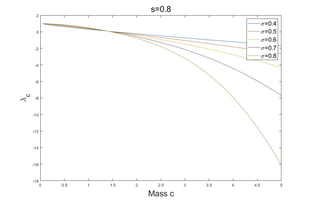
Second, we test the relationship between mass cc and λc\lambda_{c}, where cc, λc\lambda_{c} are mass and Lagrange multiplier corresponding to the minimizer (8)-(10) . By [9], in the case s=1s=1, there exits λ0\lambda_{0} such that for any σ\sigma,

limc→0λc=λ0.\lim_{c\rightarrow 0}\lambda_{c}=\lambda_{0}.

We also test this with s=0.8s=0.8. From figure (4(b)), we can see for different σ\sigma, when c→0c\rightarrow 0, λc\lambda_{c} will also converge to a same value λ0\lambda_{0}.

Refer to caption
(a) Evolution of E⁡(s)E(s) with different ss
Refer to caption
(b) Evolution of λc\lambda_{c} with different cc
Figure 4: Energy and λc\lambda_{c}

Up to now, we only consider the case with radial symmetrical potential. However, when potential is not radially symmetric, we can still find standing waves to (1) using (8). We tried the case where potential is |x|2+a​sin⁡(2​π​x)|x|^{2}+a\sin(2\pi x) with a=1a=1 and a=5a=5. From figure 5(a) and 5(b), we see if we add a nonsymmetrical perturbation to potential, we won’t get radially symmetrical ground state solutions.

Refer to caption
(a) potential term=|x|2+sin⁡(2​π​x)|x|^{2}+\sin(2\pi x)
Refer to caption
(b) potential term=|x|2+5​sin⁡(2​π​x)|x|^{2}+5\sin(2\pi x)
Figure 5: Ground state solutions with non-symmetric potential

7.2 Dynamics and stability of ground state solution

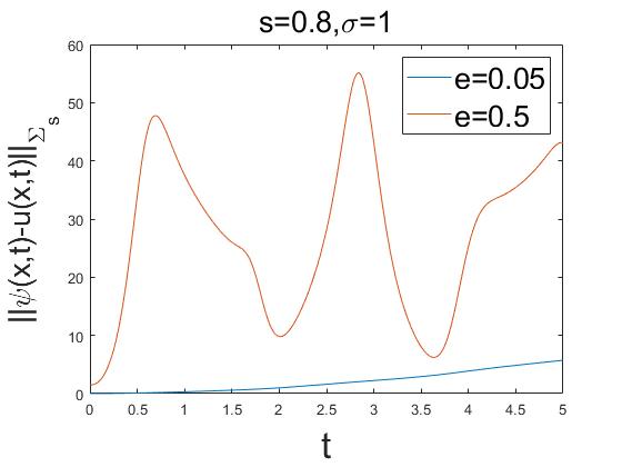
First, we consider the case s>N​σ2s>\frac{N\sigma}{2}, which is covered by our Theorem 2.2. From theoretic results and figure 1(b), we can see standing waves preserve |ψ⁡(x,t)||\psi(x,t)| with time tt. Therefore, we use |ψ⁡(x,t)||\psi(x,t)| to draw graphs and test its stability. We consider the case s=0.8s=0.8 and σ=1\sigma=1. We first test condition (36) in Theorem 2.2 with initial condition ψ0​(x)=(1+e)∗u0​(x)\psi_{0}(x)=(1+e)*u_{0}(x), because the scheme is mass preserving, it suffices to test energy preservation, which is showed in figure 6(a),6(b). Then, we test the stability of solution, where ee is a constant number. From figure 6(c),6(d), we can see when e=0.05e=0.05, the solution almost preserves |ψ⁡(x,t)||\psi(x,t)| as we desired. When e=0.2e=0.2, the solution shows large perturbation but still has periodic behavior, similar to [9] and [15]. In figure 7, we compare ∥⋅∥Σ~s\|\cdot\|_{\widetilde{\Sigma}_{s}} distance between ground state solution and perturbed solution.

Refer to caption
(a) Energy check when ψ0s​(x)=(1.05)∗u0s​(x)\psi^{s}_{0}(x)=(1.05)*u^{s}_{0}(x)
Refer to caption
(b) Energy check when ψ0s​(x)=(1.2)∗u0s​(x)\psi^{s}_{0}(x)=(1.2)*u^{s}_{0}(x)
Refer to caption
(c) Absolution value of solution when ψ0s​(x)=(1.05)∗u0s​(x)\psi^{s}_{0}(x)=(1.05)*u^{s}_{0}(x)
Refer to caption
(d) Absolution value of solution when ψ0s​(x)=(1.2)∗u0s​(x)\psi^{s}_{0}(x)=(1.2)*u^{s}_{0}(x)
Figure 6: Energy and stability check with s=0.8s=0.8, σ=1\sigma=1
Refer to caption
Figure 7: ‖ψs​(x,t)−us​(x,t)‖Σ~s\|\psi^{s}(x,t)-u^{s}(x,t)\|_{\widetilde{\Sigma}_{s}} when s=0.8s=0.8 and σ=1\sigma=1

We can see from figure 2(b) and theoretic results that when s→σ​N2s\rightarrow\frac{\sigma N}{2}, the regularity of ground state solutions becomes worse. This inspires us to investigate its stability relationship with ss. By Theorem 2.2, Def 4.1, the orbital stability means we can find ω∈𝒪~c\omega\in\widetilde{\mathcal{O}}_{c} such that ‖ω−ψ‖Σ~s​(ℝ)\|\omega-\psi\|_{\widetilde{\Sigma}_{s}(\mathbb{R})} is small when we only have small perturbation in initial condition. This definition is hard to measure. Therefore, instead of checking the exact definition of orbital stability, we test classical stability by comparing distance between perturbed solution and ground state solution using normalized ∥⋅∥Σ~s​(ℝ)\|\cdot\|_{\widetilde{\Sigma}_{s}(\mathbb{R})} distance:

D⁡(s,t)=‖us​(x,t)−ψs​(x,t)‖Σ~s​(ℝ)‖us​(x,t)‖Σ~s​(ℝ).D(s,t)=\frac{\|u^{s}(x,t)-\psi^{s}(x,t)\|_{\widetilde{\Sigma}_{s}(\mathbb{R})}}{\|u^{s}(x,t)\|_{\widetilde{\Sigma}_{s}(\mathbb{R})}}.

We test initial condition ψ0​(x)=0.9∗u0​(x)\psi_{0}(x)=0.9*u_{0}(x) with s=0.8s=0.8 and s=0.6s=0.6. From figure 8,9(a), as expected, when ss is small, its stability seems worse. To be complete, we test D⁡(s,1)D(s,1) with ss between 0.510.51 and 11 in figure 9(b). We can see D⁡(1,s)D(1,s) increases when ss approaches to 0.50.5, which implies worse stability.

Refer to caption
(a) Abosolute value of solution with ψ0s​(x)=0.9∗u0s​(x)\psi^{s}_{0}(x)=0.9*u^{s}_{0}(x) and s=0.8s=0.8
Refer to caption
(b) Abosolute value of solution with ψ0s​(x)=0.9∗u0s​(x)\psi^{s}_{0}(x)=0.9*u^{s}_{0}(x) with s=0.6s=0.6
Figure 8: Abosolute of solution with different ss
Refer to caption
(a) D⁡(0.8,t)D(0.8,t) vs D⁡(0.6,t)D(0.6,t)
Refer to caption
(b) D⁡(1,t)D(1,t) with different ss
Figure 9: Stability test with ψ0s​(x)=0.9∗u0s​(x)\psi^{s}_{0}(x)=0.9*u^{s}_{0}(x)

Second, we try to obtain some numerical result when we touch the critical point s=σ​N2s=\frac{\sigma N}{2}. In this case, we can’t find the ground state solution through (8) because Ic=−∞I_{c}=-\infty. However, as we discussed before, we can find a ground state solution related to another constrained minimization problem (62). Here, we try to use the NGF method to find the ground state solution with s=0.5s=0.5, σ=1\sigma=1. We first tried positive ω\omega, but the projection step dominated the process (68). Therefore, we tried ω=−0.5\omega=-0.5 and find the method does converge to a solution. From figure 10(b)-10(d), we can see |ψ⁡(x,t)||\psi(x,t)| almost preserves with time tt with periodical real and imaginary part. We use it to test the finite blow up phenomenon (ψ0​(x)=2​u0​(x)\psi_{0}(x)=2u_{0}(x)) appeared in the case without potential [15], and this also happens with potential (Figure 10(e)). We note here we still can’t find a perfect ground state solution, the reason might come from when s=0.5s=0.5, the stability of (1) is very bad.

Refer to caption
(a) Standing waves when s=0.5s=0.5
Refer to caption
(b) Absolute value of ground state solution w s=0.5s=0.5
Refer to caption
(c) Time evolution of R​e​(ψ⁡(0,t))Re(\psi(0,t))
Refer to caption
(d) Time evolution of I​m​(ψ⁡(0,t))Im(\psi(0,t))
Refer to caption
(e) Blow up of solution with ψ0​(x,t)=2​u0​(x)\psi_{0}(x,t)=2u_{0}(x)
Figure 10: Standing wave and ground state solution when s=0.5s=0.5, δ=1\delta=1

Finally, we test some simple time dynamics of FNLS, we let ψ0​(x)=u0​(x)​ei​k​x\psi_{0}(x)=u_{0}(x)e^{ikx}, which changes its phase but not absolute value. If s=0.8s=0.8 and k=1,20k=1,20 (Figure 11(a), 11(b)), the maximum point of |ψ⁡(x,t)||\psi(x,t)| will move along xx periodically. We also test the L∞L^{\infty} norm of ψ⁡(x,t)\psi(x,t) (Figure 11(c)). We find it decreases first and then approaches to some limits, which is similar to the case without potential [15].

Refer to caption
(a) Abolute value of solution when s=0.8,ψ0​(x)=u0​(x)​ei​xs=0.8,\psi_{0}(x)=u_{0}(x)e^{ix}.
Refer to caption
(b) Abolute value of solution when s=0.8,ψ0​(x)=u0​(x)​ei​20​xs=0.8,\psi_{0}(x)=u_{0}(x)e^{i20x}.
Refer to caption
(c) L∞L^{\infty} evolution of the solution when s=0.8,ψ0​(x)=u0​(x)​ei​20​xs=0.8,\psi_{0}(x)=u_{0}(x)e^{i20x}.
Figure 11: Dynamics of FNLS

References

  • [1] F. J. Almgren and E. H. Lieb, Symmetric decreasing rearrangement is sometimes continuous, Journal of the American Mathematical Society, 2 (1989), pp. 683–773.
  • [2] W. Bao and Q. Du, Computing the ground state solution of bose–einstein condensates by a normalized gradient flow, SIAM J. Sci. Comput., 25 (2004), pp. 1674–1697.
  • [3] R. Carles and H. Hajaiej, Complementary study of the standing wave solutions of the gross-pitaevskii equation in dipolar quantum gases, Bulletin of the London Mathematical Society, 47 (2014).
  • [4] T. Cazenave and P.-L. Lions, Orbital stability of standing waves for some nonlinear schrödinger equations, Communications in Mathematical Physics, 85 (1982).
  • [5] X. Chang, Ground state solutions of asymptotically linear fractional schrödinger equation, Journal of Mathematical Physics, 54 (2013).
  • [6] M. Cheng, Bound state for the fractional schrödinger equation with unbounded potential, Journal of Mathematical Physics, 53 (2012).
  • [7] S. Duo and Y. Zhang, Mass-conservative fourier spectral methods for solving the fractional nonlinear schrödinger equation, Computers and Mathematics with Applications, (2016).
  • [8] G. Fibich and X.-P. Wang, Stability of solitary waves for nonlinear schrödinger equations with inhomogeneous nonlinearities, Physica D: Nonlinear Phenomena, 175 (2003), p. 96–108.
  • [9] F. Hadj Selem, H. Hajaiej, P. Markowich, and S. Trabelsi, Variational approach to the orbital stability of standing waves of the gross-pitaevskii equation, Milan Journal of Mathematics, 82 (2014).
  • [10] H. Hajaiej, On the optimality of the assumptions used to prove the existence and symmetry of minimizers of some fractional constrained variational problems, Annales Henri Poincaré, 14 (2013), pp. 1425–1433.
  • [11] H. Hajaiej, P. A. Markowich, and S. Trabelsi, Minimizers of a class of constrained vectorial variational problems: Part i., Milan Journal of Mathematics, 82 (2014), pp. 81–98.
  • [12] H. Hajaiej, L. Molinet, T. Ozawa, and B. Wang, Sufficient and necessary conditions for the fractional gagliardo-nirenberg inequalities and applications to navier-stokes and generalized boson equations, RIMS Kokyuroku Bessatsu, (2010).
  • [13] H. Hajaiej and C. Stuart, On the variational approach to the stability of standing waves for the nonlinear schrödinger equation, Advanced Nonlinear Studies, 4 (2004).
  • [14] H. Hajaiej and C. A. Stuart, Symmetrization inequalities for composition operators of carathéodory type, Proceedings of the London Mathematical Society, 87 (2003), p. 396–418.
  • [15] C. Klein, C. Sparber, and P. Markowich, Numerical study of fractional nonlinear schrodinger equations, Proceedings. Mathematical, physical, and engineering sciences / the Royal Society, 470 (2014), p. 20140364.
  • [16] N. Laskin, Fractional quantum mechanics and lévy path integrals, Physics Letters A, 268 (2000), pp. 298–305.
  • [17] N. Laskin, Fractional schrödinger equation, Phys. Rev. E, 66 (2002), p. 056108.
  • [18] H. Rose and M. Weinstein, On the bound states of the nonlinear schrödinger equation with a linear potential, Physica D: Nonlinear Phenomena, 30 (1988), pp. 207–218.
  • [19] J. Zhang, Stability of standing waves for nonlinear schrödinger equations with unbounded potentials, Zeitschrift für angewandte Mathematik und Physik, 51 (2000), p. 498.
  • [20] F. Zhao, L. Zhao, and Y. Ding, Existence and multiplicity of solutions for a non-periodic schrödinger equation, Nonlinear Analysis-theory Methods and Applications, 69 (2008), pp. 3671–3678.