The strange properties of the infinite power tower
 An “investigative math” approach for young students

After presenting the infinite power tower function, its definition and its unexpected properties (section 2 - Introduction), we start an investigation about its mathematical characteristics. In section 3 (Generalization) we introduce the function $y=x^{y}$ and its inverse function $x=y^{1/y}$ that prove to be useful to give some promising clues on the infinite power tower. In section 4 (The problem of convergence) we introduce the problem of the convergence of the recursive sequence leading to the infinite power tower. This problem is furtherly investigated in the sections 5 (Fixed points and convergence criteria (in general)), 6 (Fixed points and convergence of the power tower (the algebraic route)) and 7 (Fixed points and convergence of the power tower (the graphical route)), where the investigation is brought forward with both algebraic and graphical methods. Section 8 (Outside the convergence interval) explores what happens outside the convergence interval and the emergence of a periodic cycle for the values given by the power tower function. Lastly, in section 9 (Some history about the power tower) we briefly discuss some very interesting historical aspects on the origin of the interest about the infinite power tower (where the main characters are Lambert, Euler and Lagrange).

Let’s define the “Infinite Power Tower” function (or “Tetration with infinite heights’’) as:²² 2 In the rest of this article we’ll assume that $x,y\in\Re$ and $x>0$, $y>0$

where the tower of exponentiations has an infinite height.

People aware of the explosive nature of exponential functions will guess that, if $x>1$, the $f\left(x\right)$ previously defined will soon blow up to infinity as the height of the tower is increased. But, contrary to this initial guess, some trial with a pocket calculator suggests that there might be a stable behavior for some set of values, even with $x>1$.

In fact, some numerical experiments show that if we set $x=\sqrt{2}$ , then

The reason for that can be gained by the following reasoning. Since the sequence of exponentials is infinite, adding (or removing) one element to an infinite sequence shouldn’t change its overall effect (like adding or subtracting a finite number to infinite). We can then follow the passages outlined below:

We could be tempted to extend and generalize the procedure in the following way

so that, setting $y=3$ it would be $x=3^{1\mathord{\left/{\vphantom{13}}\right.\kern-1.2pt}3}=\sqrt[3]{3}$ and setting $y=4$ it would be $x=\sqrt[4]{4}=\sqrt{2}$.

But here we have a problem: if we set $x=\sqrt{2}$ what will we get for the $y$: 2 or 4?

Let’s check again numerically.
After having defined the following recursive function in Mathematica or in Geogebra

we find that a tower with height$=$1000, starting from $x=\sqrt{2}$, yields a result of 2 (as expected, anyway not “4”), but if the starting point is $\sqrt[3]{3}$ the result is not 3 (as previously supposed), but rather a mysterious 2.47805.

The same results are confirmed when the height of the exponentiations is increased to even higher values so that we can be confident that, for these values of the $x$, there is a definite value for the $y$.
Another strange thing happens when we give the $x$ some values close to 0 and consider odd/even numbers for the height of the tower:

It seems that a small change in the height of the tower may produce a relevant change in the result. How can it be?

These initial experiments suggest the following practical questions to be addressed:

• •

  Why is $f\left({\sqrt{2}}\right)=2$ (and not 4)?

• •

  Why is not $f\left({\sqrt[3]{3}}\right)=3$?

• •

  For which values of $x$ do we have a definite (finite) value of $y$?

• •

  Why do we sometimes get two different values whit small changes in the height of the tower?

We have previously defined the infinite power tower function as:

where the tower of exponentiations has an infinite height.

Firstly, let’s make clear what is the conventional meaning of applying subsequent exponentiations.

In order to do so it’s convenient to start from the definition of the related functions representing towers with finite heights. It will be:

$y_{n}=f_{n}\left(x\right)=x^{x^{x^{x^{...}}}}$ }${}^{n\,times}$

so it is $y_{1}=f_{1}\left(x\right)=x,\,\,\,\,y_{2}=f_{2}\left(x\right)=x^{x},\,\,\,y_{3}=f_{3}\left(x\right)=x^{x^{x}}$ and so on.

It’s important to observe that it is $x^{x^{x}}=x^{\left({x^{x}}\right)}$ and not $x^{x^{x}}=\left({x^{x}}\right)^{x}=x^{x^{2}}$.

This means that the tower is built from the highest exponent downwards to the lowest level.

This example shows the difference between a downwards and an upwards construction:

Using the definition of the “finite” tower $f_{n}\left(x\right)$, the infinite power tower can then be re-defined as follows:

Alternatively, we can build the sequence of functions $\left\{{y_{1},\,\,y_{2},\,\,y_{3},\,\,y_{4},...,\,\,y_{n},...}\right\}$ and take advantage of the fact that this sequence can be defined recursively as:

It’s easy to check that with above definition we have

reproducing, when $n\to\infty$, our infinite power tower.

After having clarified the meaning of the infinite power tower function $y=f\left(x\right)$ we can say that, if it converges to some finite value $y$, than it is $y=x^{\left\{{x^{x^{x^{x^{{\mathinner{\mkern 2.0mu\raise 1.0pt\hbox{.}\mkern 2.0mu\raise 4.0pt\hbox{.}\mkern 2.0mu\raise 7.0pt\hbox{.}\mkern 1.0mu}}}}}}}\right\}=y}\to y=x^{y}$

The inverse function will then be

Unlike $y=x^{y}$ (that’s not the expression in explicit form of a function), this appears to be a well-defined function (although mapping $y\mapsto x)$ for any value $y>0$. So, let’s study the characteristics of this function $x=g\left(y\right)=y^{1\mathord{\left/{\vphantom{1y}}\right.\kern-1.2pt}y}$ to get some insight on the function $f\left(x\right)$ we are mostly interested in.

Note that we’ll use the following useful identity in some calculation: $x=y^{1\mathord{\left/{\vphantom{1y}}\right.\kern-1.2pt}y}=e^{\ln y^{1\mathord{\left/{\vphantom{1y}}\right.\kern-1.2pt}y}}=e^{l{ny}\mathord{\left/{\vphantom{{ny}y}}\right.\kern-1.2pt}y}$

Expression: $x=y^{1\mathord{\left/{\vphantom{1y}}\right.\kern-1.2pt}y}$

Domain: $y>0$

Limits: $\lim\limits_{y\to 0}y^{1\mathord{\left/{\vphantom{1y}}\right.\kern-1.2pt}y}=0^{+}\quad\lim\limits_{y\to\infty}y^{1\mathord{\left/{\vphantom{1y}}\right.\kern-1.2pt}y}=1$

in fact, using the L’Hôpital’s rule (H),
    $y^{1/y}=e^{lny/y}$ and $\mathop{\lim}\limits_{y\to{0^{+}}}\frac{{\ln y}}{y}=-\infty$, $\mathop{\lim}\limits_{y\to+\infty}\frac{{\ln y}}{y}\mathop{=}\limits^{H}0$

First derivative: $\frac{dx}{dy}=\frac{d}{dy}\left({e^{l{ny}\mathord{\left/{\vphantom{{ny}y}}\right.\kern-1.2pt}y}}\right)=e^{l{ny}\mathord{\left/{\vphantom{{ny}y}}\right.\kern-1.2pt}y}\left({\frac{1-\ln y}{y^{2}}}\right)=y^{\frac{1}{y}}\left({\frac{1-\ln y}{y^{2}}}\right)$

Asymptotes: the line $x=1$ is a horizontal asymptote

Stationary points: $\frac{dx}{dy}=0\to 1-\ln y=0\to y=e\to x=e^{1\mathord{\left/{\vphantom{1e}}\right.\kern-1.2pt}e}$

$\frac{dx}{dy}>0\to 1-\ln y>0\to y<e$ The point $M\left({y_{M};x_{M}}\right)=\left({e;e^{1\mathord{\left/{\vphantom{1e}}\right.\kern-1.2pt}e}}\right)$ is a maximum.

Second derivative: $\frac{d^{2}x}{dy^{2}}=y^{1\mathord{\left/{\vphantom{1y}}\right.\kern-1.2pt}y-4}\left({1-3y+\left({2y+\ln y-2}\right)\cdot\ln y}\right)$

Inflection points: $1-3y+\left({2y+\ln y-2}\right)\cdot\ln y=0\to\left\{{{\begin{array}[]{*{20}c}{y_{F1}\approx 0.5819,\,\,x_{F1}\approx 0.3944}\hfill\\ {y_{F2}\approx 4.3678,\,\,x_{F2}\approx 1.4015}\hfill\\ \end{array}}}\right.$

The plot of $g\left(y\right)$ is:

We must remember that in the plot above, differently from the usual conventions, the vertical axis represents the $x$ and the horizontal axis is the $y$.

If we rotate the graph we get, now with the usual orientation of the axis, the set of points satisfying the equivalent relations:

$x=y^{1\mathord{\left/{\vphantom{1y}}\right.\kern-1.2pt}y}$ or $y=x^{y}$ or $y=e^{y\,\ln x}$

But since $g\left(y\right)$ is not invertible as it is not bijective, the plot shown in Fig. 2 is not that of a function.

The inverse function of $g\left(y\right)$ could only be defined on a proper restriction of the domain of $g$, where the function is a bijection.

For example, this condition would be respected in the region defined by $0<x\leq e^{1\mathord{\left/{\vphantom{1e}}\right.\kern-1.2pt}e}\wedge y>0$ and we’d get the following plot:

The plot of Fig. 2 represents all the points satisfying the equation $y=x^{y}$. Anyway, it would be problematic to say that these points are also the ones satisfying the equation of the infinite power tower

In fact, above equation is written in the form of a function, whilst $y=x^{y}$ is not the expression of a function.

Furthermore the plot tells us that for some values of the $x$ (with $1<x<e^{1\mathord{\left/{\vphantom{1e}}\right.\kern-1.2pt}e})$ we would get two possible values of the $y$ and this doesn’t make much sense with how the $f\left(x\right)$ is defined.

The problem is hidden in the following passage:

If the infinite power tower converges than it is $y=x^{x^{x^{x^{x^{x^{x^{...}}}}}}}=x^{\left\{{x^{x^{x^{x^{x^{x^{...}}}}}}}\right\}=y}\to y=x^{y}$

But the truth is that the infinite power tower doesn’t converge for every values of $x$.

How can we tell that? And how can we find the interval of convergence?

We must recall that the function $f\left(x\right)$ can be defined by recursion as the limit of a sequence of functions with finite heights:

So, given some value of $x$, we can say that the sequence $\left\{{y_{n}}\right\}$ converges if it stabilizes to some finite value as far as $n$ is increased.

In practice, the convergence requires that $\lim\limits_{n\to\infty}y_{n+1}=y_{n}$ (or $\lim\limits_{n\to\infty}y_{n+1}-y_{n}=0).$

To find the conditions assuring the convergence of a recursive sequence we abandon temporarily our power tower function and explore, in more general terms, sequences, fixed points and when a sequence is bound to converge to a fixed point.

In general, given a sequence defined by its starting value $y_{1}$ and by the recursion equation $y_{n+1}=r\left({y_{n}}\right)$, where $r$ is a smooth function, a fixed point $y^{\ast}$ is a value satisfying the equation $y^{\ast}=r\left({y^{\ast}}\right)$. The name fixed point means that if $y_{n}=y^{\ast}$ then $y_{n+1}=r\left({y_{n}}\right)=r\left({y^{\ast}}\right)=y^{\ast}$ and the sequence will keep on re-producing the same value for all future iterations.

Once we have found the fixed point(s) of a sequence by solving the equation $y=r\left(y\right)$ we may be interested to know if a fixed point is stable (or attractive) or not.

If the fixed point is attractive then, when we start close to it, we will end up even closer. In mathematical terms we can say that, calling $\delta_{n}$ the distance between $y^{\ast}$ and $y_{n}$ ($\delta_{n}>0)$ and starting from a point $y_{n}=y^{\ast}\pm\delta_{n}$ the subsequent term will be $y_{n+1}=y^{\ast}\pm\delta_{n+1}$ , and the requirement for the convergence is that $\delta_{n+1}<\delta_{n}$ $\forall n$. Since it is

$\delta_{n+1}=\left|{y_{n+1}-y^{\ast}}\right|=\left|{r\left({y_{n}}\right)-r\left({y^{\ast}}\right)}\right|$ and $\delta_{n}=\left|{y_{n}-y^{\ast}}\right|$ we have

The closer we are to $y^{\ast}$ the more above ratio will approximate the absolute value of the derivative $\left|{{r}^{\prime}\left({y^{\ast}}\right)}\right|$. This suggests that it’s possible to use the mean value theorem to state that there exist a point $\xi\in\left({y_{n},y^{\ast}}\right)$ such that

In our case we can say that there exists a point $\xi\in\left({y_{n},y^{\ast}}\right)$ such that

Then, if there is some interval in which it is $\left|{{r}^{\prime}\left(y\right)}\right|<k<1\quad\forall y\in\left({\left|{y^{\ast}-y}\right|<\delta_{n}}\right)$ it will also be

and

that is

and so on.

We then see that if $\left|{{r}^{\prime}\left(y\right)}\right|<1$ in some neighborhood of $y^{\ast}$ and if the starting point of the recursive sequence belongs to this same neighborhood, the distance to the fixed point reduces more and more as $n$ is increased and we’ll have $\lim\limits_{n\to\infty}{\kern 1.0pt}\delta_{n}=0$ meaning that $\lim\limits_{n\to\infty}{\kern 1.0pt}y_{n}=y^{\ast}$.

In a more formal way, we state (without a complete and rigorous proof) the following theorem (fixed point convergence criteria):

The convergence/divergence character of the fixed points can be interpreted graphically with the so called “cobweb^′′ construction.

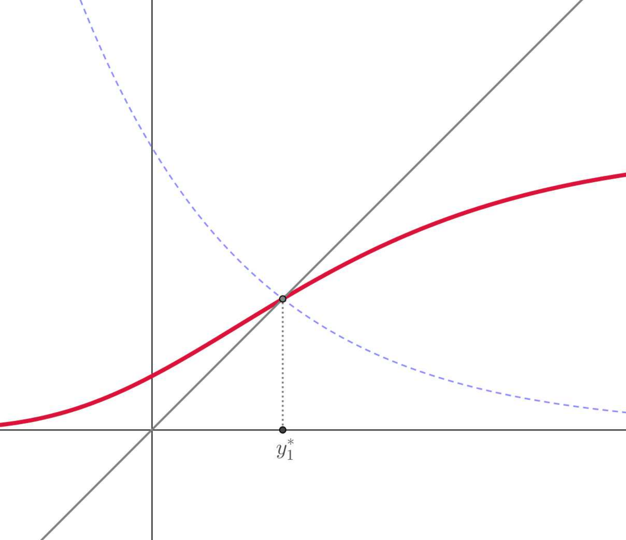
In the following Fig. 4 we have the recursion equation $y_{n+1}=r\left({y_{n}}\right)$ plotted with $y_{n+1}$ as a function of $y_{n}$. The fixed points are the intersections between $r\left({y_{n}}\right)$ and the line $y_{n+1}=y_{n}$. Here we have two fixed points labeled $P_{1}$ and $P_{2}$. The cobweb construction shows that $P_{1}$ is an attractive fixed (stable) point whilst $P_{2}$ is a repulsive (unstable) fixed point. This is due to the fact that $\left|{{r}^{\prime}\left({y_{P_{1}}}\right)}\right|<1$ and $\left|{{r}^{\prime}\left({y_{P_{2}}}\right)}\right|>1$.

In the case presented in this article we are interested in the convergence of the sequence of functions

Here the $x$ variable should be considered as a parameter of the recursion equation whose variables are the terms $y_{n}$ and $y_{n+1}$. In practice we have an infinite number of sequences, one for each value of $x$.

The fixed points $\left({y^{\ast}}\right)$ of these sequences are those for which it is $y_{n+1}=y_{n}$ that is those satisfying the equation

Using the fixed point convergence criteria we must find the interval of the values of the $y$ (and of the $x)$ for which the first derivative of $x^{y}$ has modulus less than 1, that is

For this purpose, it’s convenient to use the equivalence

$x^{y}=e^{\ln x^{y}}=e^{y\ln x}$ and calculate the following derivative, with respect to $y$:

Using the fact that for the fixed points it is $y=x^{y}$ we have

For the convergence it must then be $\left|{\ln y}\right|<1$, that is

The corresponding values for the $x$ (since it is $x=y^{1\mathord{\left/{\vphantom{1y}}\right.\kern-1.2pt}y})$ are then $e^{-e}$ and $e^{1\mathord{\left/{\vphantom{1e}}\right.\kern-1.2pt}e}$ .

Then, if we use the fixed point convergence criteria, we can say that the convergence is assured for

producing stable fixed points in the interval

To gain a deepest understanding of what the previous result actually means, we now switch to another route more rich of visual elements.

In the case of the sequence $y_{n+1}=x^{y_{n}}$ we see that the recursion equation is a family of exponential curves (think of the “$x$” as a parameter) and the search of the possible fixed points and their stability is rather simplified, mostly because these functions are strictly monotonic (apart the banal case with $x=1)$.

In order to simplify the notation let’s rename the variables as follows:

Then, we want to study the family of exponential functions

(where the base $x$ can be considered a parameter).

With this notation a fixed point $y^{\ast}$ is the solution of the system $\left\{{{\begin{array}[]{ll}{z=x^{y}}\\ {z=y}\\ \end{array}}}\right.$ leading to the equation $y=x^{y}$.

The character of the exponential is determined by the value of its base $x$:

• •

  $x>1:$ the exponential is increasing;

• •

  $x=1:$ the exponential becomes the constant line $z=1$ and the original infinite power tower function becomes $y=1^{1^{1^{{\mathinner{\mkern 2.0mu\raise 1.0pt\hbox{.}\mkern 2.0mu\raise 4.0pt\hbox{.}\mkern 2.0mu\raise 7.0pt\hbox{.}\mkern 1.0mu}}}}}=1$;

• •

  $x<1:$ the exponential is decreasing;

The positions of the curves defined by the recursive function $z=x^{y}$ with respect to the identity line $z=y$ allow us to determine the possible existence of fixed points.

With $x>1$ we may have the following cases (Fig. 5):

I) The exponential curve is always above the line: there are no fixed points.
II) The exponential curve is tangent to the line: there is one single fixed point $y_{1}^{\ast}$ (or two coincident fixed points).
III) The exponential curve intersects the line in two points: there are two distinct fixed points $y_{1}^{\ast}$ and $y_{2}^{\ast}$.

With $x<1$ (decreasing exponential) there will always be a single intersection point and a single corresponding fixed point. We’ll distinguish the following cases (Fig. 6):

IV) The first derivative in the intersection point is $-1\leq\frac{d}{dy}\left({x^{y}}\right)\leq 0$

V) The first derivative in the intersection point is $\frac{d}{dy}\left({x^{y}}\right)<-1$

Now we’ll examine above 5 cases, analyze the characteristics of the fixed points and find which values of the “$x$” produce them.

If $x>1$ the discriminating case is that for which the exponential is tangent to the line (Fig. 7).

So, let’s look for the tangency point $T$. In this point the exponential will have the same slope of the line, that is $z^{\prime}\left(y\right)=\frac{d}{dy}\left({x^{y}}\right)=1$.
Then

and

We have found the point $T\left({-\frac{\ln\ln x}{\ln x},\frac{1}{\ln x}}\right)$ in which it is $z^{\prime}\left(y\right)=1$. But for the exponential curve to be tangent to the line $z=y$ we must impose that $T$ belong to that line, that is

With this value the exponential function becomes $z=\left({e^{1\mathord{\left/{\vphantom{1e}}\right.\kern-1.2pt}e}}\right)^{y}$ and the point of tangency is $T\left({e,e}\right)$.

Knowing how the base influences the graphic of a generic exponential curve we can also say that:

If $x>e^{1\mathord{\left/{\vphantom{1e}}\right.\kern-1.2pt}e}$ there’s no intersection (and no fixed points for the recursive sequence).

If $x=e^{1\mathord{\left/{\vphantom{1e}}\right.\kern-1.2pt}e}$ there is a single intersection (and a single fixed point for the recursive sequence).

If $1<x<e^{1\mathord{\left/{\vphantom{1e}}\right.\kern-1.2pt}e}$ there are two intersections (and two fixed points for the recursive sequence).

With the cobweb diagram we can see what evolution the sequence will follow in these cases:

If $x>e^{1\mathord{\left/{\vphantom{1e}}\right.\kern-1.2pt}e}$ (Fig. 9) there is no fixed point and, with any starting point, the sequence is bound to diverge to infinity.

If $x=e^{1\mathord{\left/{\vphantom{1e}}\right.\kern-1.2pt}e}$ (Fig. 9) the cobweb iterations converge to $P_{1}\quad\left({e,e}\right)$ if the starting value is to the left of $P_{1}$ and diverge if the starting value is to the right. We can say that $P_{1}$ is a “half-stable” saddle fixed point. Anyway, for the power tower sequence the starting value is $y_{0}=x=e^{1\mathord{\left/{\vphantom{1e}}\right.\kern-1.2pt}e}$ that is located to the left of $P_{1}\left({e,e}\right)$. So the sequence converge to $y^{\ast}=e$.

If $1<x<e^{1\mathord{\left/{\vphantom{1e}}\right.\kern-1.2pt}e}$ there are two fixed points that are the solutions of the of equation $y=x^{y}$. Let’s call them $y^{\ast}_{1}$ and $y^{\ast}_{2}$(Fig. 10).

The cobweb iterations show that $y^{\ast}_{1}$ is attractive and $y^{\ast}_{2}$ is repulsive. Furthermore the sequence will converge to $y^{\ast}_{1}$ for any starting point $y_{0}<y^{\ast}_{2}$ and diverge to infinity for $y_{0}>y^{\ast}_{2}$. Anyway, for the power tower sequence the starting value is $y_{0}=x$ and it’s located to the left of $y^{\ast}_{1}$. In fact, for the fixed point holds the relation $y^{\ast}_{1}=x^{y^{\ast}_{1}}\to x=\left({y^{\ast}_{1}}\right)^{1\mathord{\left/{\vphantom{1{y^{\ast}_{1}}}}\right.\kern-1.2pt}{y^{\ast}_{1}}}$ and if we set $x<y^{\ast}_{1}$ it must be $\left({y^{\ast}_{1}}\right)^{1\mathord{\left/{\vphantom{1{y^{\ast}_{1}}}}\right.\kern-1.2pt}{y^{\ast}_{1}}}<y^{\ast}_{1}$. Taking the logarithms of both sides we have $\ln\left({y^{\ast}_{1}}\right)^{1\mathord{\left/{\vphantom{1{y^{\ast}_{1}}}}\right.\kern-1.2pt}{y^{\ast}_{1}}}<\ln y^{\ast}_{1}$ that is $1\mathord{\left/{\vphantom{1{y^{\ast}_{1}}}}\right.\kern-1.2pt}{y^{\ast}_{1}}\ln\left({y^{\ast}_{1}}\right)<\ln y^{\ast}_{1}\to 1\mathord{\left/{\vphantom{1{y^{\ast}_{1}}}}\right.\kern-1.2pt}{y^{\ast}_{1}}<1\to y^{\ast}_{1}>1$.

So it is $x<y^{\ast}_{1}$ if $y^{\ast}_{1}>1$. But since $z=x^{y}$ is increasing and it’s $z\left(0\right)=1$, the first intersection of the exponential with the line $z=y$ must have a value $z>1$. This implies (since $y=z)$ that $y>1$. So it is $y^{\ast}_{1}>1$ and $x<y^{\ast}_{1}$. The sequence converges to $y^{\ast}_{1}$.

To complete our analysis let’s see what happens with $0<x<1$. In this case the exponential curve $z=x^{y}$ is decreasing and there can be only one single intersection point with the line $z=y$ and a corresponding single fixed point. Anyway some interesting unexpected things are going to happen when we start analyzing the stability of that fixed point and the eventual convergence of the sequence to it.

Two different cobweb iteration are presented for this case in the following figures, producing rather different outcomes. If the first derivative is $\left|{z^{\prime}\left({y^{\ast}_{1}}\right)}\right|<1$ (that is $-1\leq z^{\prime}\left({y^{\ast}_{1}}\right)<0$, Fig. 12) the iterations converge to $y^{\ast}_{1}$, oscillating between values alternatively greater and less than that of the fixed point. We can say that the fixed point is attractive and that the sequence will eventually converge to it, whatever is the starting point.

On the contrary, if the first derivative is $\left|{z^{\prime}\left({y^{\ast}_{1}}\right)}\right|>1$ (that is $z^{\prime}\left({y^{\ast}_{1}}\right)<-1$, Fig. 12) the iterations are again oscillating but the sequence doesn’t converge to $y^{\ast}_{1}$ . Instead it stabilizes towards a periodic stable cycle, getting closer and closer to two alternate distinct fixed values.

Let’s then see for what value of $x$ we have $z^{\prime}\left({y^{\ast}_{1}}\right)>-1$. Since we have already found that $z^{\prime}\left({y^{\ast}_{1}}\right)=x^{y}\ln x$ we must solve the inequality $x^{y}\ln x>-1$ with $y=x^{y}$ meaning $x=y^{1\mathord{\left/{\vphantom{1y}}\right.\kern-1.2pt}y}$. It will then be

We can then say that the fixed point is attractive for $e^{-e}\leq x<1$ and that we’ll have a 2-cycle for $0<x<e^{-e}$.

What can we say about the two values $y_{1}$ and $y_{2}$ involved in the 2-cycle?

Since $y_{2}$ is the next value in the sequence after $y_{1}$ and $y_{1}$ is the next value in the sequence after $y_{2}$ we have $y_{2}=x^{y_{1}}$ and $y_{1}=x^{y_{2}}$. Let’s take the power $y_{1}$ of both sides of the second equation to get $y_{1}^{y_{1}}=x^{y_{2}y_{1}}$.

Inserting $x^{y_{1}}=y_{2}$ we have $y_{1}^{y_{1}}=y_{2}^{y_{2}}$ and $y_{1}\ln y_{1}=y_{2}\ln y_{2}$.

Let’s now say that $y_{2}$ is $p$ times $y_{1}$, that is $y_{2}=py_{1}$ and solve for $y_{1}$.

We finally have

For instance, if we set $p=2$ we have $y_{1}=1\mathord{\left/{\vphantom{14}}\right.\kern-1.2pt}4$ and $y_{2}=1\mathord{\left/{\vphantom{12}}\right.\kern-1.2pt}2$. These are the two values of the cycle that we’d get with $x=y_{2}^{1\mathord{\left/{\vphantom{1y}}\right.\kern-1.2pt}y_{1}}=y_{1}^{1\mathord{\left/{\vphantom{1y}}\right.\kern-1.2pt}y_{2}}=\left({1\mathord{\left/{\vphantom{12}}\right.\kern-1.2pt}2}\right)^{4}=\left({1\mathord{\left/{\vphantom{14}}\right.\kern-1.2pt}4}\right)^{2}=1\mathord{\left/{\vphantom{1{16=0.0625}}}\right.\kern-1.2pt}{16=0.0625}$. We can also find the two values for the extreme cycle in which $y_{1}$ and $y_{2}$ have the maximum separation. Setting $p\to\infty$ we have

and, since $y_{1}=x^{y_{2}}$, $0=x^{1},\,\,\,x\to 0$.

The following table summarizes the results gained so far.

It’s interesting to note that how the number $e$ appears in above table in many possible power variations.

In conclusion, we can now say that the infinite power tower converges to the function defined by the expression $y=x^{y}$ (or $x=y^{1\mathord{\left/{\vphantom{1y}}\right.\kern-1.2pt}y}$ ) for $e^{-e}\leq x\leq e^{1\mathord{\left/{\vphantom{1e}}\right.\kern-1.2pt}e}$ assuming values $1\mathord{\left/{\vphantom{1e}}\right.\kern-1.2pt}e\leq y\leq e$.

Taking into account the information collected we can show, in Fig. 13, the final plot of the infinite power tower function.

We have seen that the infinite power tower converges for $e^{-e}\leq x\leq e^{1\mathord{\left/{\vphantom{1e}}\right.\kern-1.2pt}e}$, assuming values $1\mathord{\left/{\vphantom{1e}}\right.\kern-1.2pt}e\leq y\leq e$.

But what happens outside the convergence interval?

Let’s try some numerical experiment with some power towers with finite (but rather high) height.

For $x>e^{1\mathord{\left/{\vphantom{1e}}\right.\kern-1.2pt}e}$ the function $f\left(x\right)$ blows out rapidly to $+\infty$ (Fig. 14). In fact we already know that there aren’t fixed points for the sequence $y_{n+1}=x^{y_{n}}$ when we use $x>e^{1\mathord{\left/{\vphantom{1e}}\right.\kern-1.2pt}e}$ .

As we have already seen, for $0<x<e^{-e}$ the sequence start to oscillate between two bounded values, and some numerical simulation confirms that behavior (Fig. 15). The upper/lower branches of the plot correspond to an even/odd value for the height of the tower.

We have already seen this oscillating behavior when exploring, through the cobweb diagrams, the recursive sequence $y_{n+1}=x^{y_{n}}$ with $x<e^{-e}$.

Let’s analyze further the origin of this feature.

First we can try to calculate the limit of the finite power tower when $x\to 0$. Let’s start with $f_{2}$:

we can now calculate the limit of the exponent (using the L’Hôpital’s rule)

so it is

Then we are on the upper branch. What changes when we increase the tower height?

and since $\lim\limits_{x\to 0}x^{x}=1$, as seen before, the last limit has the form $0^{1}\to 0$

So it is $\lim\limits_{x\to 0}f_{2}\left(x\right)=\lim\limits_{x\to 0}x^{x}=1$ and $\lim\limits_{x\to 0}f_{3}\left(x\right)=\lim\limits_{x\to 0}x^{x^{x}}=0$.

We have a strong suspect (supported by the previous reasoning based on the cobweb diagrams) that these results may extend to towers with any height, with different values for $n$ even and $n$ odd, that is $\lim\limits_{x\to 0}f_{2n}\left(x\right)=1$ and $\lim\limits_{x\to 0}f_{2n+1}\left(x\right)=0$ but we can’t prove this conjecture with simple tools and leave this problem to a later time.

Having observed the oscillating character of the finite power tower sequence for $0<x<e^{-e}$, we ask ourselves if it’s possible to find the equations of the two distinct branches.

Calling $a$ and $b$ the two values corresponding to some $\bar{{x}}$ it must be:

This means that the sequence built with a double recursion should converge to its fixed points $a$ and $b$.

Let’s see what is the form of this double recursion:

This sequence has stable fixed points if the derivative with respect to $y$ of the right side has modulus less than 1, that is

Since it is $x^{x^{y}}=e^{\ln x^{x^{y}}}=e^{x^{y}\ln x}$ the derivative to calculate becomes:

after some passage we arrive at

and it must be

Differently from before we can’t find an explicit algebraic form for the boundary of the region of convergence.

Anyway, using the RegionPlot command of Mathematica we can visualize it (Fig. 16). The double step sequence converges in the gray region and does not in the white one.

In the gray region, where the double step sequence converge, it will converge to the sequence whose fixed points are given by the transcendental equation

Now we can now put all the pieces together.

In Fig. 17 we can see the plots $p_{1}$ and $p_{2}$ defined by the equations $y=x^{y}$ and $y=x^{x^{y}}$respectively. These equations are also the equations defining the fixed points of the sequences $s_{1}:y_{n+1}=x^{y_{n}}$ and $s_{2}:y_{n+2}=x^{x^{y_{n}}}$. The gray region is where both sequences converge (“c” in the figure), while the white area (“d1” in the figure) is a region where there’s no convergence. The blue line is produced by both equations (since the fixed points of a “single iteration” sequence are also fixed points for the one with a “double iteration” step). At the left of the line $x=e^{-e}$ (“d2” in the figure) there’s no convergence for $s_{1}$ and we have three branches. The upper and lower branches (in red) are produced only by the equation $y=x^{x^{y}}$.
Since they lie in a region of convergence for this sequence their values can be also produced by the infinite power tower function and we’ll have alternating values, one on the upper branch (for even heights of the tower) and the other on the lower branch (odd values of the heights). The middle branch represent points produced by both equations. Anyway this branch is entirely located in the region “d1” where there is no convergence for both $s_{1}$ and $s_{2}$. The infinite power tower won’t assume these values.

Fig. 18 shows an enlargement of the region with the three branches.

Now we can find an answer to our previously unanswered question: what is the limit of the infinite power tower function when $x\to 0$?

The answer is: that limit doesn’t exist. In fact, more precisely, we can have two distinct values for that limit.

That’s because, since in the converging region it is $y=x^{x^{y}}$, we have