Explicit results have so far only been obtained for de Sitter background, which corresponds to $\epsilon=0$, with $H$ exactly constant. Suppose the inflaton $\varphi$ is Yukawa-coupled to a massless, Dirac fermion on this background via the interaction $\mathcal{L}_{\rm Yukawa}=-\lambda\varphi\overline{\psi}\psi\sqrt{-g}$. The one loop correction to the inflaton effective potential on de Sitter was originally derived by Candelas and Raine in 1975 [10]. Of course their result depends slightly on conventions of regularization and renormalization. Our more recent computation [11] employed dimensional regularization in $D$ spacetime dimensions with conformal and quartic counterterms,

$$\Delta\mathcal{L}^{f}=-\frac{1}{2}\delta\xi^{f}\varphi^{2}R\sqrt{-g}-\frac{1}{4!}\delta\lambda^{f}\varphi^{4}\sqrt{-g}\;.$$

(3)

To simplify the result we took the dimensional regularization scale $\mu$ to be proportional to the constant Hubble parameter of de Sitter,

	$\displaystyle\delta\xi^{f}_{0}$	$\displaystyle=$	$\displaystyle\frac{4\lambda^{2}H^{D-4}}{(4\pi)^{\frac{D}{2}}}\Biggl\{\frac{\Gamma(1\!-\!\frac{D}{2})}{D(D\!-\!1)}+\frac{(1\!-\!\gamma)}{6}+O(D\!-\!4)\Biggr\}\;,$		(4)
	$\displaystyle\delta\lambda^{f}_{0}$	$\displaystyle=$	$\displaystyle\frac{24\lambda^{4}H^{D-4}}{(4\pi)^{\frac{D}{2}}}\Biggl\{\Gamma\Bigl(1\!-\!\frac{D}{2}\Bigr)+2\zeta(3)-2\gamma+O(D\!-\!4)\Biggr\}\;,$		(5)

where $\gamma=0.577...$ is the Euler-Mascheroni constant. These choices result in a cosmological Coleman-Weinberg potential of the form $\Delta V^{f}_{0}(\varphi,H)=-\frac{H^{4}}{8\pi^{2}}\times f(z)$, where $z\equiv\frac{\lambda\varphi}{H}$, and the function $f(z)$ is,

$$f(z)=2\gamma z^{2}-[\zeta(3)\!-\!\gamma]z^{4}+2\!\!\int_{0}^{z}\!\!\!\!dx\,(x\!+\!x^{3})\Bigl[\psi(1\!+\!ix)+\psi(1\!-\!ix)\Bigr]\;,$$

(6)

and $\psi(x)\equiv\frac{d}{dx}\ln[\Gamma(x)]$ is the digamma function.

We assume that de Sitter results can be extended to general homogeneous and siotropic geometries (2) by simply replacing the constant de Sitter Hubble parameter with the time dependent $H(t)$ for a general background. However, we must be careful to keep the dimensional regularization scale constant, which amounts to a small change of the counterterms (4-5),

	$\displaystyle\delta\xi^{f}_{1}$	$\displaystyle=$	$\displaystyle\frac{4\lambda^{2}\mu^{D-4}}{(4\pi)^{\frac{D}{2}}}\Biggl\{\frac{\Gamma(1\!-\!\frac{D}{2})}{D(D\!-\!1)}+\frac{(1\!-\!\gamma)}{6}+O(D\!-\!4)\Biggr\}\;,$		(7)
	$\displaystyle\delta\lambda^{f}_{1}$	$\displaystyle=$	$\displaystyle\frac{24\lambda^{4}\mu^{D-4}}{(4\pi)^{\frac{D}{2}}}\Biggl\{\Gamma\Bigl(1\!-\!\frac{D}{2}\Bigr)+2\zeta(3)-2\gamma+O(D\!-\!4)\Biggr\}\;.$		(8)

The net effect is to change $\Delta V^{f}_{0}(\varphi,H)$ to,

$$\Delta V^{f}_{1}(\varphi,H)=-\frac{H^{4}}{8\pi^{2}}\Biggl\{f(z)+z^{2}\ln\Bigl(\frac{H^{2}}{\mu^{2}}\Bigr)+\frac{1}{2}z^{4}\ln\Bigl(\frac{H^{2}}{\mu^{2}}\Bigr)\Biggr\}\;.$$

(9)

The contribution of a gauge boson to a charged inflaton,

$$\mathcal{L}_{\rm vector}=-\Bigl(\partial_{\mu}+ieA_{\mu}\Bigr)\varphi^{*}\Bigl(\partial_{\nu}-ieA_{\nu}\Bigr)\varphi g^{\mu\nu}\sqrt{-g}\;,$$

(10)

was originally computed on de Sitter background using mode sums by Allen in 1983 [12]. As always, the precise result depends on conventions of regularization and renormalization. Our more recent, dimensionally regulated computation [13] employed the massive photon propagator [14] with conformal and quartic counterterms,

$$\Delta\mathcal{L}^{b}=-\delta\xi^{b}\varphi^{*}\varphi R\sqrt{-g}-\frac{1}{4}\delta\lambda^{b}(\varphi^{*}\varphi)^{2}\sqrt{-g}\;.$$

(11)

We again chose the dimensional regularization mass scale $\mu$ to be proportional to the constant de Sitter Hubble parameter,

	$\displaystyle\delta\xi^{b}_{0}$	$\displaystyle=$	$\displaystyle\frac{e^{2}H^{D-4}}{(4\pi)^{\frac{D}{2}}}\Biggl\{\frac{1}{4\!-\!D}+\frac{1}{2}\gamma+O(D\!-\!4)\Biggr\}\;,$		(12)
	$\displaystyle\delta\lambda^{b}_{0}$	$\displaystyle=$	$\displaystyle\frac{D(D\!-\!1)e^{4}H^{D-4}}{(4\pi)^{\frac{D}{2}}}\Biggl\{\frac{2}{4\!-\!D}+\gamma-\frac{3}{2}+O(D\!-\!4)\Biggr\}\;,$		(13)

These choices result in a cosmological Coleman-Weinberg potential of the form $\Delta V^{b}_{0}(\varphi^{*}\varphi,H^{2})=+\frac{3H^{4}}{8\pi^{2}}\times b(z)$, where $z\equiv\frac{e^{2}\varphi^{*}\varphi}{H^{2}}$, and $b(z)$ is,

	$\displaystyle b(z)=\Bigl(-1\!+\!2\gamma\Bigr)z+\Bigl(-\frac{3}{2}\!+\!\gamma\Bigr)z^{2}$				(14)
			$\displaystyle\hskip 56.9055pt+\!\int_{0}^{z}\!\!\!\!dx\,(1\!+\!x)\Biggl[\psi\Bigl(\frac{3}{2}\!+\!\frac{1}{2}\sqrt{1\!-\!8x}\,\Bigr)+\psi\Bigl(\frac{3}{2}\!-\!\frac{1}{2}\sqrt{1\!-\!8x}\,\Bigr)\Biggr]\;.\qquad$

When generalizing the constant de Sitter Hubble parameter to the time-dependent one of a general homogeneous and isotropic geometry we must revise the counterterms (12-13) to keep the mass scale of dimensional regularization strictly constant,

	$\displaystyle\delta\xi^{b}_{1}$	$\displaystyle=$	$\displaystyle\frac{e^{2}\mu^{D-4}}{(4\pi)^{\frac{D}{2}}}\Biggl\{\frac{1}{4\!-\!D}+\frac{1}{2}\gamma+O(D\!-\!4)\Biggr\}\;,$		(15)
	$\displaystyle\delta\lambda^{b}_{1}$	$\displaystyle=$	$\displaystyle\frac{D(D\!-\!1)e^{4}\mu^{D-4}}{(4\pi)^{\frac{D}{2}}}\Biggl\{\frac{2}{4\!-\!D}+\gamma-\frac{3}{2}+O(D\!-\!4)\Biggr\}\;.$		(16)

The net effect is to change $\Delta V^{b}_{0}(\varphi^{*}\varphi,H^{2})$ to,

$$\Delta V^{b}_{1}(\varphi^{*}\varphi,H^{2})=+\frac{3H^{4}}{8\pi^{2}}\Biggl\{b(z)+z\ln\Bigl(\frac{H^{2}}{\mu^{2}}\Bigr)+\frac{1}{2}z^{2}\ln\Bigl(\frac{H^{2}}{\mu^{2}}\Bigr)\Biggr\}\;.$$

(17)

Ricci subtraction amounts to subtracting the primitive contribution with the replacement $H^{2}(t)\rightarrow\frac{1}{12}R(t)$. In a homogeneous and isotropic geometry this can be thought of as an $\epsilon$-dependent Hubble parameter $\overline{H}(t)$,

$$R(t)=12H^{2}(t)+6\dot{H}(t)=12\Bigl[1-\frac{1}{2}\epsilon(t)\Bigr]H^{2}(t)\equiv 12\overline{H}^{2}(t)\;.$$

(18)

Because the quartic terms cancel between the primitive potential and the Ricci subtraction, the full fermionic result takes the form $\Delta V^{f}_{2}(\varphi,H)-\Delta V^{f}_{2}(\varphi,\overline{H})$ where,

	$\displaystyle\Delta V^{f}_{2}(\varphi,H)$	$\displaystyle\!\!=\!\!$	$\displaystyle-\frac{H^{4}}{8\pi^{2}}\Biggl\{\Delta f(z)+z^{2}\ln\Bigl(\frac{H^{2}}{H^{2}_{\rm inf}}\Bigr)\Biggr\}\quad,\quad z\equiv\frac{\lambda\varphi}{H}\;,$		(19)
	$\displaystyle\Delta f(z)$	$\displaystyle\!\!=\!\!$	$\displaystyle 2\gamma z^{2}-\frac{1}{2}z^{4}\ln(z^{2})+2\!\!\int_{0}^{z}\!\!\!\!dx\,(x\!+\!x^{3})\Bigl[\psi(1\!+\!ix)+\psi(1\!-\!ix)\Bigr]\;.\qquad$		(20)

Note that we have chosen the constant mass scale to be the Hubble parameter at the beginning of inflation, $\mu=H_{\rm inf}$. The full bosonic result takes the form $\Delta V^{b}_{2}(\varphi^{*}\varphi,H^{2})-\Delta V^{b}_{2}(\varphi^{*}\varphi,\overline{H}^{2})$ where,

	$\displaystyle\Delta V^{b}_{2}(\varphi^{*}\varphi,H^{2})$	$\displaystyle=$	$\displaystyle+\frac{3H^{4}}{8\pi^{2}}\Biggl\{\Delta b(z)+z\ln\Bigl(\frac{H^{2}}{H^{2}_{\rm inf}}\Bigr)\Biggr\}\quad,\quad z\equiv\frac{e^{2}\varphi^{*}\varphi}{H^{2}}\;,$		(21)
	$\displaystyle\Delta b(z)$	$\displaystyle=$	$\displaystyle\Bigl(-1\!+\!2\gamma\Bigr)z-\frac{1}{2}z^{2}\ln(2z)$		(22)
			$\displaystyle\hskip-14.22636pt+\!\!\int_{0}^{z}\!\!\!\!dx\,(1\!+\!x)\Biggl[\psi\Bigl(\frac{3}{2}\!+\!\frac{1}{2}\sqrt{1\!-\!8x}\,\Bigr)+\psi\Bigl(\frac{3}{2}\!-\!\frac{1}{2}\sqrt{1\!-\!8x}\,\Bigr)\Biggr]\;.\qquad$

The Ricci subtraction scheme for fermionic corrections is defined by the potentials,

	$\displaystyle U^{f}(\phi,\chi)$	$\displaystyle=$	$\displaystyle\frac{1}{2}k^{2}\phi^{2}-\frac{\chi^{4}}{8\pi^{2}}\Biggl[\Delta f\Bigl(\frac{\lambda\phi}{\chi}\Bigr)+\Bigl(\frac{\lambda\phi}{\chi}\Bigr)^{2}\ln\Bigl(\frac{\chi^{2}}{\chi^{2}(0)}\Bigr)\Biggr]\;,$		(39)
	$\displaystyle U^{f}_{\rm sub}(\phi,\overline{\chi})$	$\displaystyle=$	$\displaystyle+\frac{\overline{\chi}^{4}}{8\pi^{2}}\Biggl[\Delta f\Bigl(\frac{\lambda\phi}{\overline{\chi}}\Bigr)+\Bigl(\frac{\lambda\phi}{\overline{\chi}}\Bigr)^{2}\ln\Bigl(\frac{\overline{\chi}^{2}}{\chi^{2}(0)}\Bigr)\Biggr]\;,$		(40)

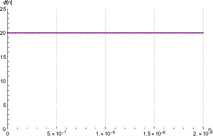
where $\Delta f(z)$ was defined in (20) and $\overline{\chi}\equiv\sqrt{1-\frac{1}{2}\epsilon}\,\chi$. Figure 1 displays the classical evolution (in blue) versus the quantum-corrected model (in red dots) for a moderate coupling of $\lambda=5.5\times 10^{-4}$.

To understand why Ricci subtraction engenders immediate deviations for $\lambda=5.5\times 10^{-4}$, first note that the initial conditions of the classical model (34-35) force the initial value of the parameter $z\equiv\frac{\lambda\phi}{\chi}$ to be much larger than one,

$$z_{0}=\frac{\lambda\phi_{0}}{\chi_{0}}=\frac{\lambda}{k}\sqrt{6-(\frac{2}{\phi_{0}})^{2}}\simeq 220\;.$$

(41)

This means it is valid to use the large $z$ expansion of (20) [8],

$$\Delta f(z)=-\frac{1}{4}z^{4}+z^{2}\ln(z^{2})-\Bigl(\frac{5}{6}\!-\!2\gamma\Bigr)z^{2}+\frac{11}{60}\ln(z^{2})+O(1)\;.$$

(42)

Substituting (42) in expressions (39-40) implies,

	$\displaystyle U^{f}(\phi,\chi)$	$\displaystyle=$	$\displaystyle\frac{1}{2}k^{2}\phi^{2}-\frac{\chi^{4}}{8\pi^{2}}\Biggl\{-\frac{1}{4}\Bigl(\frac{\lambda\phi}{\chi}\Bigr)^{4}+\Bigl[\ln\Bigl(\frac{\lambda^{2}\phi^{2}}{\chi_{0}^{2}}\Bigr)\!-\!\frac{5}{6}\!+\!2\gamma\Bigr]\Bigl(\frac{\lambda\phi}{\chi}\Bigr)^{2}$		(43)
			$\displaystyle\hskip 170.71652pt+\frac{11}{60}\ln\Bigl(\frac{\lambda^{2}\phi^{2}}{\chi^{2}}\Bigr)+\dots\Biggr\},\qquad$
	$\displaystyle U^{f}_{\rm sub}(\phi,\overline{\chi})$	$\displaystyle=$	$\displaystyle\frac{\overline{\chi}^{4}}{8\pi^{2}}\Biggl\{-\frac{1}{4}\Bigl(\frac{\lambda\phi}{\overline{\chi}}\Bigr)^{4}+\Bigl[\ln\Bigl(\frac{\lambda^{2}\phi^{2}}{\chi_{0}^{2}}\Bigr)\!-\!\frac{5}{6}\!+\!2\gamma\Bigr]\Bigl(\frac{\lambda\phi}{\overline{\chi}}\Bigr)^{2}$		(44)
			$\displaystyle\hskip 170.71652pt+\frac{11}{60}\ln\Bigl(\frac{\lambda^{2}\phi^{2}}{\overline{\chi}^{2}}\Bigr)+\dots\Biggr\}.\qquad$

The $(\lambda\phi)^{4}$ terms cancel out between (43) and (44) so that the leading contribution usually comes from the $(\lambda\phi)^{2}$ term,

	$\displaystyle U^{f}+U^{f}_{\rm sub}-\chi^{2}\Biggl[2\frac{\partial U^{f}}{\partial\chi^{2}}+\frac{1}{2}(1\!-\!\epsilon)\frac{\partial U^{f}_{\rm sub}}{\partial\overline{\chi}^{2}}\Biggr]$				(45)
			$\displaystyle\hskip 85.35826pt=\frac{1}{2}k^{2}\phi^{2}+\frac{\chi^{4}}{8\pi^{2}}\!\times\!\frac{3}{2}z^{2}\Biggl[\ln\Bigl(\frac{\lambda^{2}\phi^{2}}{\chi_{0}^{2}}\Bigr)\!-\!\frac{5}{6}\!+\!2\gamma\Biggr]+\dots\qquad$
	$\displaystyle\frac{1}{2}\chi^{2}\phi^{\prime}\,\frac{\partial^{2}U^{f}_{\rm sub}}{\partial\phi\partial\overline{\chi}^{2}}=\frac{\chi^{4}}{8\pi^{2}}\!\times\!\frac{\phi^{\prime}}{\phi}z^{2}\Biggl[\ln\Bigl(\frac{\lambda^{2}\phi^{2}}{\chi_{0}^{2}}\Bigr)\!+\!\frac{1}{6}\!+\!2\gamma\Biggr]+\dots$				(46)

However, the $(\lambda\phi)^{2}$ term makes no contribution to the denominator, so one must go one order higher,

$$\chi^{4}\frac{\partial^{2}U^{f}_{\rm sub}}{\partial\overline{\chi}^{4}}=\frac{\chi^{4}}{8\pi^{2}}\!\times\!\frac{11}{60}\Biggl[2\ln\Bigl(\frac{\lambda^{2}\phi^{2}}{\overline{\chi}^{2}}\Bigr)-3\Biggr]+\dots$$

(47)

Taking account of the fact that the classical terms initially cancel, and that $\phi_{0}^{\prime}/\phi_{0}=-\epsilon_{0}$, the large $z_{0}$ form of (32) is,

$$\epsilon_{0}^{\prime}\simeq-4\epsilon_{0}+2\epsilon_{0}^{2}+\frac{6z_{0}^{2}[\ln(z_{0}^{2})\!-\!\frac{5}{6}\!+\!2\gamma]-4\epsilon_{0}z_{0}^{2}[\ln(z_{0}^{2})\!+\!\frac{1}{6}\!+\!2\gamma]}{\frac{11}{60}[2\ln(z_{0}^{2})\!-\!2\ln(1\!-\!\frac{1}{2}\epsilon_{0})\!-\!3]}\simeq 9.4\times 10^{5}\;.$$

(48)

This compares with the slow roll result of $\epsilon^{\prime}_{0}=2\epsilon_{0}^{2}=5\times 10^{-5}$, and explains why the subtraction term brings inflation to such an abrupt end.

Because the large fraction in (48) scales like $\lambda^{2}$ one might expect that decreasing $\lambda$ reduces $\epsilon^{\prime}(0)$. This is indeed true for as long as the large $z$ regime pertains, but $\epsilon^{\prime}(0)$ approaches a constant value of about 6 in the small $z$ regime, as can be seen from Figure 2.

To understand the small $z$ limit of $\epsilon^{\prime}(0)$, note first that the small $z$ expansion of $\Delta f(z)$ is [8],

$$\Delta f(z)=-\frac{1}{2}z^{4}\ln(z^{2})+\Bigl[\zeta(3)-\gamma\Bigr]z^{4}+\frac{2}{3}\Bigl[\zeta(3)-\zeta(5)\Bigr]z^{6}+O(z^{8})\;.$$

(49)

Comparison with expressions (39) and (40) implies that the small $\lambda$ limiting forms derive from the conformal renormalization,

	$\displaystyle U^{f}(\phi,\chi)-\frac{1}{2}k^{2}\phi^{2}$	$\displaystyle\longrightarrow$	$\displaystyle-\frac{\lambda^{2}\phi^{2}\chi^{2}}{8\pi^{2}}\ln\Bigl(\frac{\chi^{2}}{\chi_{0}^{2}}\Bigr)\;,$		(50)
	$\displaystyle U^{f}_{\rm sub}(\phi,\overline{\chi})$	$\displaystyle\longrightarrow$	$\displaystyle+\frac{\lambda^{2}\phi^{2}\overline{\chi}^{2}}{8\pi^{2}}\ln\Bigl(\frac{\overline{\chi}^{2}}{\chi_{0}^{2}}\Bigr)\;.$		(51)

Substituting (50-51) in the final term of (32) gives,

$$\epsilon^{\prime}_{0}\longrightarrow-4\epsilon_{0}+2\epsilon_{0}^{2}+\frac{6\!-\!2\epsilon_{0}\!+\!2(1\!-\!2\epsilon_{0})\ln(1\!-\!\frac{1}{2}\epsilon_{0})}{(1\!-\!\frac{1}{2}\epsilon_{0})^{-1}}\;.$$

(52)

A striking feature of Figure 2 and expression (52) is that the limit $\lambda\rightarrow 0$ fails to agree with the case of $\lambda=0$ for which there is no change to classical inflation. This seems contradictory but is in fact the standard signature of a perturbation that changes the number of derivatives. A simple example is the higher derivative extension of the simple harmonic oscillator considered in section 2.2 of [16]. The oscillator’s position is $x(t)$ and its Lagrangian is,

$$L=-\frac{\epsilon m}{2\omega^{2}}\ddot{x}^{2}+\frac{m}{2}\dot{x}^{2}-\frac{m\omega^{2}}{2}x^{2}\;.$$

(53)

When $\epsilon=0$ this system reduces to the simple harmonic oscillator which has two pieces of initial value data and whose energy is bounded below. However, for any nonzero value of $\epsilon$ the system has four pieces of initial value data, and its energy is unbounded below. Because the effect of the higher derivative perturbation (in our inflation model) never becomes small, no matter how small the coupling constant, it follows that perturbation theory breaks down.

Making the inflaton complex causes a few small changes in the key equations of section 3. Because the two potentials $U^{b}(\phi^{*}\phi,\chi^{2})$ and $U^{b}_{\rm sub}(\phi^{*}\phi,\overline{\chi}^{2})$ depend on the norm-squared of the scalar, the evolution equation for the inflaton becomes,

$$\chi^{2}\Bigl[\phi^{\prime\prime}+(3\!-\!\epsilon)\phi^{\prime}\Bigr]+\phi\Biggl[\frac{\partial U^{b}(\phi^{*}\phi,\chi^{2})}{\partial\phi^{*}\phi}+\frac{\partial U^{b}_{\rm sub}(\phi^{*}\phi,\overline{\chi}^{2})}{\partial\phi^{*}\phi}\Biggr]=0\;.$$

(54)

The first Friedmann equation takes the form,

$$3\chi^{2}=\chi^{2}{\phi^{\prime}}^{*}\phi^{\prime}+U^{b}+U^{b}_{\rm sub}-\chi^{2}\Biggl[2\frac{\partial U^{b}}{\partial\chi^{2}}+\frac{1}{2}(1\!-\!\epsilon)\frac{\partial U^{b}_{\rm sub}}{\partial\overline{\chi}^{2}}\Biggr]+\frac{1}{2}\chi^{2}\frac{d}{dn}\frac{\partial U^{b}_{\rm sub}}{\partial\overline{\chi}^{2}}\;.$$

(55)

This gives an evolution equation for the first slow roll parameter analogous to (32),

	$\displaystyle\epsilon^{\prime}=-4\epsilon+2\epsilon^{2}+\frac{4}{\chi^{4}\frac{\partial^{2}U^{b}_{\rm sub}}{\partial\overline{\chi}^{4}}}\Biggl\{-\chi^{2}\Bigl[3\!-\!{\phi^{\prime}}^{*}\phi^{\prime}\Bigr]+U^{b}+U^{b}_{\rm sub}$				(56)
			$\displaystyle\hskip 71.13188pt-\chi^{2}\Biggl[2\frac{\partial U^{b}}{\partial\chi^{2}}+\frac{1}{2}(1\!-\!\epsilon)\frac{\partial U^{b}_{\rm sub}}{\partial\overline{\chi}^{2}}\Biggr]+\frac{1}{2}\chi^{2}(\phi^{*}\phi)^{\prime}\frac{\partial^{2}U^{b}_{\rm sub}}{\partial\phi^{*}\phi\partial\overline{\chi}^{2}}\Biggr\}.\qquad$

Even though we do not use it, the second Friedmann equation is,

	$\displaystyle-(3\!-\!2\epsilon)\chi^{2}=\chi^{2}{\phi^{\prime}}^{*}\phi^{\prime}-U^{b}-U^{b}_{\rm sub}+\chi^{2}\Biggl[2\frac{\partial U^{b}}{\partial\chi^{2}}+\frac{1}{2}\Bigl(1\!-\!\frac{1}{3}\epsilon\Bigr)\frac{\partial U^{b}_{\rm sub}}{\partial\overline{\chi}^{2}}\Biggr]$				(57)
			$\displaystyle\hskip 99.58464pt+\frac{1}{3}\chi^{2}\Bigl[\frac{d}{dn}\!-\!\epsilon\Bigr]\frac{\partial U^{b}}{\partial\chi^{2}}-\frac{1}{6}\chi^{2}\Bigl[\frac{d}{dn}\!+\!2\!-\!\epsilon\Bigr]\frac{d}{dn}\frac{\partial U^{b}_{\rm sub}}{\partial\overline{\chi}^{2}}\;.\qquad$

And the initial values (assuming $\phi_{0}$ is real) become,

	$\displaystyle\phi(0)=\phi_{0}\qquad$	,	$\displaystyle\qquad\phi^{\prime}(0)=-\frac{2}{\phi_{0}}\;,$		(58)
	$\displaystyle\chi(0)=\frac{k\phi_{0}}{\sqrt{3\!-\!(\frac{2}{\phi_{0}})^{2}}}\qquad$	,	$\displaystyle\qquad\chi^{\prime}(0)=-\frac{2\chi_{0}}{\phi_{0}^{2}}\;.$		(59)

We continue to use $\phi_{0}=20$, with the value of $k$ given in (38).

The Ricci subtraction scheme for bosons is defined by these potentials,

	$\displaystyle U^{b}(\phi^{*}\phi,\chi^{2})$	$\displaystyle=$	$\displaystyle k^{2}\phi^{*}\phi+\frac{3\chi^{4}}{8\pi^{2}}\Biggl[\Delta b\Bigl(\frac{e^{2}\phi^{*}\phi}{\chi^{2}}\Bigr)+\frac{e^{2}\phi^{*}\phi}{\chi^{2}}\ln\Bigl(\frac{\chi^{2}}{\chi^{2}(0)}\Bigr)\Biggr]\;,$		(60)
	$\displaystyle U^{b}_{\rm sub}(\phi^{*}\phi,\overline{\chi}^{2})$	$\displaystyle=$	$\displaystyle-\frac{3\overline{\chi}^{4}}{8\pi^{2}}\Biggl[\Delta b\Bigl(\frac{e^{2}\phi^{*}\phi}{\overline{\chi}^{2}}\Bigr)+\frac{e^{2}\phi^{*}\phi}{\overline{\chi}^{2}}\ln\Bigl(\frac{\overline{\chi}^{2}}{\chi^{2}(0)}\Bigr)\Biggr]\;,$		(61)

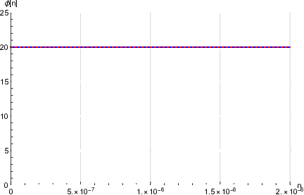
where $\Delta b(z)$ was defined in (22) and $\overline{\chi}\equiv\sqrt{1-\frac{1}{2}\epsilon}\,\chi$. Figure 3 compares the classical evolution (in blue) with the quantum-corrected (in red dots) for a charge $e^{2}\simeq 2.9\times 10^{-10}$ which is three hundred million times weaker than electromagnetism.

The rapid onset of deviations from classical evolution evident in Figure 3 has the same explanation for bosons as for fermions. Even for the small coupling $e^{2}\simeq 2.9\times 10^{-10}$ the initial value of $z=\frac{e^{2}\phi^{*}\phi}{\chi^{2}}$ is larger than one,

$$z_{0}\equiv\frac{e^{2}\phi_{0}^{2}}{\chi_{0}^{2}}=\frac{e^{2}}{k^{2}}\Bigl[3-\frac{4}{\phi_{0}^{2}}\Bigr]\simeq 23.1\;.$$

(62)

Just as for fermions, this means we can simplify relation (56) using the large $z$ expansion of $\Delta b(z)$ [8],

$$\Delta b(z)=-\frac{1}{4}z^{2}+z\ln(2z)-\Bigl(\frac{5}{3}\!-\!2\gamma\Bigr)z+\frac{19}{60}\ln(z)+O(1)\;.$$

(63)

The corresponding large argument expansions of the potentials are,

	$\displaystyle U^{b}(\phi^{*}\phi,\chi^{2})$	$\displaystyle=$	$\displaystyle k^{2}\phi^{*}\phi+\frac{3\chi^{4}}{8\pi^{2}}\Biggl\{-\frac{1}{4}\Bigl(\frac{e^{2}\phi^{*}\phi}{\chi^{2}}\Bigr)^{2}$		(64)
			$\displaystyle\hskip-8.5359pt+\Bigl[\ln\Bigl(\frac{2e^{2}\phi^{*}\phi}{\chi_{0}^{2}}\Bigr)\!-\!\frac{5}{3}\!+\!2\gamma\Bigr]\frac{e^{2}\phi^{*}\phi}{\chi^{2}}+\frac{19}{60}\ln\Bigl(\frac{e^{2}\phi^{*}\phi}{\chi^{2}}\Bigr)+\dots\Biggr\},\qquad$
	$\displaystyle U^{b}_{\rm sub}(\phi^{*}\phi,\overline{\chi}^{2})$	$\displaystyle=$	$\displaystyle-\frac{3\overline{\chi}^{4}}{8\pi^{2}}\Biggl\{-\frac{1}{4}\Bigl(\frac{e^{2}\phi^{*}\phi}{\overline{\chi}^{2}}\Bigr)^{2}$		(65)
			$\displaystyle\hskip-8.5359pt+\Bigl[\ln\Bigl(\frac{2e^{2}\phi^{*}\phi}{\chi_{0}^{2}}\Bigr)\!-\!\frac{5}{3}\!+\!2\gamma\Bigr]\frac{e^{2}\phi^{*}\phi}{\overline{\chi}^{2}}+\frac{19}{60}\ln\Bigl(\frac{e^{2}\phi^{*}\phi}{\overline{\chi}^{2}}\Bigr)+\dots\Biggr\}.\qquad$

Just as for fermions, the order $e^{2}\phi^{*}\phi$ terms in (64-65) make the dominant contributions to the numerator of expression (56), but the denominator is a crucial order weaker,

$$\epsilon_{0}^{\prime}\simeq-4\epsilon_{0}+2\epsilon_{0}^{2}+\frac{6z_{0}[\ln(2z_{0})\!-\!\frac{5}{3}\!+\!2\gamma]-4\epsilon_{0}z_{0}[\ln(2z_{0})\!-\!\frac{2}{3}\!+\!2\gamma]}{\frac{19}{60}[2\ln(z_{0})\!-\!2\ln(1\!-\!\frac{1}{2}\epsilon_{0})\!-\!3]}\simeq 441\;.$$

(66)

References

• [1] Y. Akrami et al. [Planck Collaboration], arXiv:1807.06211 [astro-ph.CO].
• [2] A. Ijjas, P. J. Steinhardt and A. Loeb, Phys. Lett. B 723, 261 (2013) doi:10.1016/j.physletb.2013.05.023 [arXiv:1304.2785 [astro-ph.CO]].
• [3] A. H. Guth, D. I. Kaiser and Y. Nomura, Phys. Lett. B 733, 112 (2014) doi:10.1016/j.physletb.2014.03.020 [arXiv:1312.7619 [astro-ph.CO]].
• [4] A. Linde, doi:10.1093/acprof:oso/9780198728856.003.0006 arXiv:1402.0526 [hep-th].
• [5] A. Ijjas, P. J. Steinhardt and A. Loeb, Phys. Lett. B 736, 142 (2014) doi:10.1016/j.physletb.2014.07.012 [arXiv:1402.6980 [astro-ph.CO]].
• [6] S. R. Coleman and E. J. Weinberg, Phys. Rev. D 7, 1888 (1973). doi:10.1103/PhysRevD.7.1888
• [7] D. R. Green, Phys. Rev. D 76, 103504 (2007) doi:10.1103/PhysRevD.76.103504 [arXiv:0707.3832 [hep-th]].
• [8] S. P. Miao and R. P. Woodard, JCAP 1509, no. 09, 022 (2015) doi:10.1088/1475-7516/2015/09/022, 10.1088/1475-7516/2015/9/022 [arXiv:1506.07306 [astro-ph.CO]].
• [9] J. H. Liao, S. P. Miao and R. P. Woodard, Phys. Rev. D 99, no. 10, 103522 (2019) doi:10.1103/PhysRevD.99.103522 [arXiv:1806.02533 [gr-qc]].
• [10] P. Candelas and D. J. Raine, Phys. Rev. D 12, 965 (1975). doi:10.1103/PhysRevD.12.965
• [11] S. P. Miao and R. P. Woodard, Phys. Rev. D 74, 044019 (2006) doi:10.1103/PhysRevD.74.044019 [gr-qc/0602110].
• [12] B. Allen, Nucl. Phys. B 226, 228 (1983). doi:10.1016/0550-3213(83)90470-4
• [13] T. Prokopec, N. C. Tsamis and R. P. Woodard, Annals Phys. 323, 1324 (2008) doi:10.1016/j.aop.2007.08.008 [arXiv:0707.0847 [gr-qc]].
• [14] N. C. Tsamis and R. P. Woodard, J. Math. Phys. 48, 052306 (2007) doi:10.1063/1.2738361 [gr-qc/0608069].
• [15] N. Aghanim et al. [Planck Collaboration], arXiv:1807.06209 [astro-ph.CO].
• [16] R. P. Woodard, Scholarpedia 10, no. 8, 32243 (2015) doi:10.4249/scholarpedia.32243 [arXiv:1506.02210 [hep-th]].
• [17] R. P. Woodard, Lect. Notes Phys. 720, 403 (2007) doi:10.1007/978-3-540-71013-4_14 [astro-ph/0601672].
• [18] A. Kyriazis, S. P. Miao, N. C. Tsamis and R. P. Woodard, arXiv:1908.03814 [gr-qc].