Self-Exciting Multifractional Processes

Fabian A. Harang Marc Lagunas-Merino Salvador Ortiz-Latorre

Date: August 11, 2026

Abstract.

We propose a new multifractional stochastic process which allows for self-exciting behavior, similar to what can be seen for example in earthquakes and other self-organizing phenomena. The process can be seen as an extension of a multifractional Brownian motion, where the Hurst function is dependent on the past of the process. We define this through a stochastic Volterra equation, and we prove existence and uniqueness of this equation, as well as give bounds on the $p-$ order moments, for all $p\geq 1$ . We show convergence of an Euler-Maruyama scheme for the process, and also give the rate of convergence, which is depending on the self-exciting dynamics of the process. Moreover, we discuss different applications of this process, and give examples of different functions to model self-exciting behavior.

1. Introduction and Notation

In recent years, higher computer power and better tools from statistics show that there are many natural phenomena which do not follow the standard normal distribution, but rather exhibit different types of memory, and sometimes changing these properties over time. Therefore several different types of extensions of standard stochastic processes have been proposed to try to give a more realistic picture of nature corresponding to what we observe. There are several stochastic processes which are popular today for the modeling of varying memory in a process, one of them is known as the Hawkes process, see for example [9]. This is a point process which allows for self-exciting behavior by letting the conditional intensity to be dependent on the past events of the process. In this note, we will consider a continuous type of process which is inspired by the multifractional Brownian motion. This process is interesting for being a non-stationary Gaussian process which has regularity properties changing in time. A simple version of this process is known as the Riemann-Liouville multifractional Brownian motion and can be represented by the integral

(1.1)

B_{t}^{h}=\int_{0}^{t}\left(t-s\right)^{h\left(t\right)-\frac{1}{2}}dB_{s},

where $\left\{B_{t}\right\}_{t\in[0,T]}$ is a Brownian motion and $h$ is a deterministic function. Interestingly, if we restrict the process to a small interval, say $\left[t-\epsilon,t+\epsilon\right]$ , the local $\alpha$ -Hölder regularity of this process on that interval is of order $\alpha\sim h(t)$ if $\epsilon$ is sufficiently small. Thus the regularity of the process is depending on time. Applications of such processes have been found in fields ranging from Internet traffic and image synthesis to finance, see for example [2, 3, 4, 5, 6, 8, 11, 12]. In 2010 D. Sornette and V. Filimonov proposed a self-excited multifractal process to be considered in the modeling of earthquakes and financial market crashes, see [13]. By self-excited process, the authors mean a process where the future state depends directly on all the past states of the process. The model they proposed was defined in a discrete manner. They also suggested a possible continuous time version of their model, but they did not study its existence rigorously. This article is therefore meant as an attempt to propose a continuous time version of a similar model to that proposed by Sornette and Filimonov, and we will study its mathematical properties.

We will first consider an extension of a multifractional Brownian process, which is found as the solution to the stochastic differential equation

(1.2)

X_{t}^{h}=\int_{0}^{t}\left(t-s\right)^{h(t,X_{s}^{h})-\frac{1}{2}}dB_{s},

where $\left\{B_{t}\right\}_{t\in[0,T]}$ is a general $d$ -dimensional Brownian motion, and $h$ is bounded and takes values in $(0,1)$ . Already at this point we could think that the local regularity of the process $X$ would be depending on the history of $X$ through $h$ , in a similar manner as for the multifractional Brownian motion in equation (1.1). As we can see, the formulation of the process is through a stochastic Volterra equation with a possibly singular kernel. We will therefore show the existence and uniqueness of this equation, and then say that its solution is a Self-Exciting Multifractional Process (SEM) $X^{h}$ . We will study the probabilistic properties, and discuss examples of functions $h$ which give different dynamics for the process $X^{h}$ . The process is neither stationary nor Gaussian in general, and is therefore mathematically challenging to apply in any standard model for example in finance but do, at this point, have some interesting properties on its own. The study of such processes could also shed some light on natural phenomena behaving outside of the scope of standard stochastic processes, such as the self-excited dynamics of earthquakes as they argue in [13].

We will first show the existence and uniqueness of the Equation (1.2) and then study probabilistic and path properties such as variance and regularity of the process. We will introduce an Euler-Maruyama scheme to approximate the process, and show its strong convergence as well as estimate its rate of convergence. Finally, we will discuss an extension of the process to a Gamma type process, which might be interesting for various applications.

1.1. Notation and preliminaries

Let $T>0$ be a fixed constant. We will use the standard notation $L^{\infty}\left(\left[0,T\right]\right)$ for essentially bounded functions on the interval $\left[0,T\right]$ . Furthermore, let $\triangle^{(m)}\left[a,b\right]$ denote the $m$ -simplex. That is, define $\triangle^{(m)}[a,b]$ to be given by

\triangle^{(m)}\left([a,b]\right):=\left\{(s_{m},\ldots,s_{1}):a\leq s_{1}<\ldots<s_{m}\leq b\right\}.

We will consider functions $k:\triangle^{\left(2\right)}\left(\left[0,T\right]\right)\rightarrow\mathbb{R}_{+}$ which will be used as a kernel in an integral operator, in the sense that we consider integrals of the form

\int_{0}^{t}k\left(t,s\right)f\left(s\right)ds,

whenever the integral is well defined. We call these functions Volterra kernels.

Definition 1.

Let $k:\triangle^{(2)}\left(\left[0,T\right]\right)\rightarrow\mathbb{R}_{+}$ be a Volterra kernel. If $k$ satisfies

t\mapsto\int_{0}^{t}k\left(t,s\right)ds\in L^{\infty}\left(\left[0,T\right]\right)

and

\limsup_{\epsilon\downarrow 0}\parallel\int_{\cdot}^{\cdot+\epsilon}k\left(\cdot+\epsilon,s\right)ds\parallel_{L^{\infty}\left(\left[0,T\right]\right)}=0,

then we say that $k\in\mathcal{K}_{0}.$

We will frequently use the constant $C$ to denote a general constant, which might vary throughout the text. When it is important, we will mention what this constant depends upon in subscript, i.e. $C=C_{T}$ to denote dependence in $T$ .

2. Zhang’s Existence and Uniqueness of Stochastic Volterra Equations

In this section we will assume that $\left\{B_{t}\right\}_{t\in\left[0,T\right]}$ is a $d$ -dimensional Brownian motion defined on a filtered probability space $(\Omega,\mathcal{F},\left\{\mathcal{F}_{t}\right\}_{t\in\left[0,T\right]},P)$ . Consider the following Volterra equation

(2.1)

X_{t}=g\left(t\right)+\int_{0}^{t}\sigma\left(t,s,X_{s}\right)dB_{s},\qquad 0\leq t\leq T,

where $g$ is a measurable, $\left\{\mathcal{F}_{t}\right\}$ -adapted stochastic process and $\sigma:\triangle^{(2)}\left(\left[0,T\right]\right)\times\mathbb{R}^{n}\rightarrow\mathcal{L}\left(\mathbb{R}^{d},\mathbb{R}^{n}\right)$ is a measurable function, where $\mathcal{L}\left(\mathbb{R}^{d},\mathbb{R}^{n}\right)$ is the linear space of $d\times n$ -matrices.

Next we write a simplified version of the hypotheses for $\sigma$ and $g$ , introduced previously by Zhang in [16], which will be used to prove that there exists a unique solution to the equation $\left(\ref{eq:Stoch Volterra equation}\right)$ .

(H1):

There exists $k_{1}\in\mathcal{K}_{0}$ such that the function $\sigma$ satisfies the following linear growth inequality for all $(s,t)\in\triangle^{(2)}\left([0,T]\right),$ and $x\in\mathbb{R}^{n}$ ,

\left|\sigma\left(t,s,x\right)\right|^{2}\leq k_{1}\left(t,s\right)\left(1+\left|x\right|^{2}\right).

(H2):

There exists $k_{2}\in\mathcal{K}_{0}$ such that the function $\sigma$ satisfies the following Lipschitz inequality for all $(s,t)\in\triangle^{(2)}\left([0,T]\right),$ $x,y\in\mathbb{R}^{n}$ ,

\left|\sigma\left(t,s,x\right)-\sigma\left(t,s,y\right)\right|^{2}\leq k_{2}\left(t,s\right)\left|x-y\right|^{2}.

(H3):

For some $p\geq 2$ , we have

\sup_{t\in\left[0,T\right]}\int_{0}^{t}\left[k_{1}\left(t,s\right)+k_{2}\left(t,s\right)\right]\cdot\mathbb{E}\left[\left|g\left(s\right)\right|^{p}\right]ds<\infty,

where $k_{1}$ and $k_{2}$ satisfy $\mathbf{H1}$ and $\mathbf{H2}.$

Based on the above hypotheses, we can use the following tailor made version of the theorem on existence and uniqueness found in [16] to show that there exists a unique solution to equation $\left(\ref{eq:Stoch Volterra equation}\right)$ .

Theorem 2.

$\left(\textnormal{Xicheng Zhang}\right)$ Assume that $\sigma:\triangle^{(2)}\left([0,T]\right)\times\mathbb{R}^{n}\rightarrow\mathcal{L}\left(\mathbb{R}^{d},\mathbb{R}^{n}\right)$ is measurable, and $g$ is an $\mathbb{R}^{n}$ -valued, $\left\{\mathcal{F}_{t}\right\}$ -adapted process satisfying $\mathbf{H1}-\mathbf{H3}$ . Then there exists a unique measurable, $\mathbb{R}^{n}$ -valued, $\left\{\mathcal{F}_{t}\right\}$ -adapted process $X_{t}$ satisfying for all $t\in[0,T]$ the equation

X_{t}=g\left(t\right)+\int_{0}^{t}\sigma\left(t,s,X_{s}\right)dB_{s}.

Furthermore, for some $C_{T,p,k_{1}}>0$ we have that

\mathbb{E}\left[\left|X_{t}\right|^{p}\right]\leq C_{T,p,k_{1}}\left(1+\mathbb{E}\left[\left|g\left(t\right)\right|^{p}\right]+\sup_{t\in[0,T]}\int_{0}^{t}k_{1}\left(t,s\right)\mathbb{E}\left[\left|g\left(s\right)\right|^{p}\right]ds\right),

where $p$ is from $\mathbf{H3}.$

It will also be useful, in future sections, to consider the following additional hypothesis.

(H4):

The process $g$ is continuous and satisfies for some $\delta>0$ and for any $p\geq 2$ ,

\mathbb{E}\left[\sup_{t\in\left[0,T\right]}\left|g\left(t\right)\right|^{p}\right]<\infty,

and

\mathbb{E}\left[\left|g\left(t\right)-g\left(s\right)\right|^{p}\right]\leq C_{T,p}\left|t-s\right|^{\delta p}.

3. Self-Exciting Multifractional Stochastic Processes

Consider the stochastic process given formally by the Volterra equation

X_{t}^{h}=g\left(t\right)+\int_{0}^{t}\left(t-s\right)^{h\left(t,X_{s}^{h}\right)-\frac{1}{2}}dB_{s},

where $g$ is an $\left\{\mathcal{F}_{t}\right\}$ -adapted, one-dimensional process, $h:\left[0,T\right]\times\mathbb{R}\rightarrow\mathbb{R}_{+}$ and $B$ is a one-dimensional Brownian motion. In this section, we will show the existence and uniqueness of the solution for the above equation by means of Theorem 2. Moreover, we will discuss the continuity properties of the solution.

Definition 3.

We say that a function $h:\left[0,T\right]\times\mathbb{R}\rightarrow\mathbb{R}_{+}$ is a Hurst function with parameters $(h_{*},h^{*})$ , where $h_{*}\leq h^{*}$ , if $h\left(t,x\right)$ takes values in $\left[h_{*},h^{*}\right]\subset\left(0,1\right)$ for all $x\in\mathbb{R}^{d}$ and $t\in\left[0,T\right]$ and $h$ satisfies the following Lipschitz conditions for all $x,y\in\mathbb{R}$ and $t,t^{\prime}\in\left[0,T\right]$

\left|h\left(t,x\right)-h\left(t,y\right)\right|\leq C\left|x-y\right|,

\left|h\left(t,x\right)-h\left(t^{\prime},x\right)\right|\leq C\left|t-t^{\prime}\right|,

for some $C>0$ .

Lemma 4.

Let $\sigma\left(t,s,x\right)=\left(t-s\right)^{h(t,x)-\frac{1}{2}}$ and let $h$ be a Hurst function with parameters $(h_{*},h^{*})$ . Then

(3.1)

\left|\sigma\left(t,s,x\right)\right|^{2}\leq k\left(t,s\right)\left(1+\left|x\right|^{2}\right),

where

k\left(t,s\right)=C_{T}\left(t-s\right)^{2h_{*}-1},

and

(3.2)

\left|\sigma\left(t,s,x\right)-\sigma\left(t,s,y\right)\right|^{2}\leq C_{T}k\left(t,s\right)\left|\log\left(t-s\right)\right|^{2}\left|x-y\right|^{2}.

Moreover, $\sigma$ satisfies $\mathbf{H1}$ - $\mathbf{H2}$ .

Proof.

We prove the three claims in the order they are stated in Lemma 4, and start to prove equation $\left(\ref{eq:sigma linear growth}\right)$ . Remember that

h\left(t,x\right)\in\left[h_{*},h^{*}\right]\subset\left(0,1\right),

for all $t\in[0,T]$ and $x\in\mathbb{R}$ , therefore we can trivially find

(3.3)

\left|\sigma\left(t,s,x\right)\right|^{2}=\left(t-s\right)^{2h(t,x)-1}=\left(t-s\right)^{2\left(h(t,x)-h_{*}\right)+2h_{*}-1}\leq T^{2\left(h^{*}-h_{*}\right)}\left(t-s\right)^{2h_{*}-1},

which yields equation $\left(\ref{eq:sigma linear growth}\right)$ with $k\left(t,s\right)=C_{T}\left(t-s\right)^{2h_{*}-1}$ . Next we consider equation $\left(\ref{eq:Lipschitz sigma}\right)$ , and using that $x=\exp\left(\log\left(x\right)\right),$ we write

\sigma\left(t,s,x\right)=\exp\left(\left(\log\left(t-s\right)\right)\left(h(t,x)-\frac{1}{2}\right)\right),

where $(t,s)\in\triangle^{(2)}\left(\left[0,T\right]\right)$ and consider the following inequality derived from the fundamental theorem of calculus

(3.4)

\left|e^{x}-e^{y}\right|\leq e^{\max(x,y)}\left|x-y\right|,\qquad x,y\in\mathbb{R}.

Using the Lipschitz assumption on $h$ together with the above inequality, we have that

		$\displaystyle\left\|\sigma\left(t,s,x\right)-\sigma\left(t,s,y\right)\right\|^{2}$
		$\displaystyle\leq\exp\left(2\max\left(\log\left(t-s\right)\left(h\left(t,x\right)-\frac{1}{2}\right),\log\left(t-s\right)\left(h\left(t,y\right)-\frac{1}{2}\right)\right)\right)$
		$\displaystyle\quad\times\left\|\log\left(t-s\right)\right\|^{2}\left\|h\left(t,x\right)-h\left(t,y\right)\right\|^{2}$
		$\displaystyle\leq C^{2}\exp\left(\max\left(\log\left(t-s\right)\left(2h\left(t,x\right)-1\right),\log\left(t-s\right)\left(2h\left(t,y\right)-1\right)\right)\right)$
		$\displaystyle\quad\times\left\|\log\left(t-s\right)\right\|^{2}\left\|x-y\right\|^{2}.$

If $\left|t-s\right|\geq 1$ then

\left|\sigma\left(t,s,x\right)-\sigma\left(t,s,y\right)\right|^{2}\leq C_{T}\left|x-y\right|^{2},

since $h$ is bounded. If $\left|t-s\right|<1$ then $\log\left(t-s\right)<0$ and, using that if $\theta<0$ then $\max\left(\theta x,\theta y\right)=\theta\min\left(x,y\right)$ , we have

		$\displaystyle\left\|\sigma\left(t,s,x\right)-\sigma\left(t,s,y\right)\right\|^{2}$
		$\displaystyle\leq C^{2}\exp\left(\log\left(t-s\right)\min\left(\left(2h\left(t,x\right)-1\right),\left(2h\left(t,y\right)-1\right)\right)\right)\left\|\log\left(t-s\right)\right\|^{2}\left\|x-y\right\|^{2}$
		$\displaystyle\leq C^{2}\left\|t-s\right\|^{2h_{*}-1}\left\|\log\left(t-s\right)\right\|^{2}\left\|x-y\right\|^{2}.$

These estimates yield equation $\left(\ref{eq:Lipschitz sigma}\right)$ .

Let $k$ be defined as above and $\nu\geq 0$ . Then, for any $0\leq a<T$ , $0\leq t<T-a$ and $\delta\in\left(0,1\right)$ fixed we have

	$\displaystyle\phi_{\nu}\left(t,a\right)$	$\displaystyle:=\int_{a}^{a+t}k\left(a+t,s\right)\left\|\log\left(a+t-s\right)\right\|^{2\nu}ds$
		$\displaystyle\leq C_{T}\int_{a}^{a+t}\left(a+t-s\right)^{\left(2h_{*}-1\right)}\left\|\log\left(a+t-s\right)\right\|^{2\nu}ds$
		$\displaystyle=C_{T}\int_{0}^{t}u^{2h_{*}-1}\left\|\log\left(u\right)\right\|^{2\nu}du$
		$\displaystyle\leq C_{T}C_{T,\delta}^{2\nu}\int_{0}^{t}u^{2h_{}-1-2\nu\delta}du=C_{T,\delta,\nu,h_{}}t^{2\left(h_{*}-\nu\delta\right)},$

where we have used that $\left|\log\left(u\right)\right|\leq C_{T,\delta}u^{-\delta}$ for some constant $C_{T,\delta}>0$ . Note that $2\left(h_{*}-\nu\delta\right)>0$ if and only if $h_{*}>\nu\delta$ . Therefore, choosing $a=0$ , we have that

t\mapsto\int_{0}^{t}k\left(t,s\right)\left|\log\left(t-s\right)\right|^{2\nu}ds\in L^{\infty}\left(\left[0,T\right]\right),

if $h_{*}>0$ , for $\nu=0$ , and if $h_{*}>\delta$ , for $\nu=1$ . Furthermore, by setting $a=t^{\prime}$ and $t=\epsilon$ in the estimate for $\phi_{\nu}\left(t,a\right)$ , we have

\displaystyle\limsup_{\epsilon\rightarrow 0}

\displaystyle\parallel\int_{\cdot}^{\cdot+\epsilon}k\left(\cdot+\varepsilon,s\right)\left|\log\left(\cdot+\varepsilon-s\right)\right|^{2\nu}ds\parallel_{L^{\infty}\left(\left[0,T\right]\right)}\leq\limsup_{\epsilon\rightarrow 0}C_{T,\delta,\nu,h_{*}}\varepsilon^{2\left(h_{*}-\nu\delta\right)}=0,

if $h^{*}>0$ , for $\nu=0$ , and if $h_{*}>\delta$ , for $\nu=1$ . Since $\delta$ can be chosen arbitrarily close to zero then $h_{*}$ can be arbitrarily close to zero. These estimates yield that $\sigma$ satisfies $\mathbf{H1\text{-}H3}$ . ∎

Now, we can give the following theorem showing that the self-exciting multifractional process from equation $\left(\ref{eq:SEM}\right)$ indeed exists and is unique.

Theorem 5.

Let $\sigma\left(t,s,x\right)=\left(t-s\right)^{h(t,x)-\frac{1}{2}}$ and $h$ be a Hurst function with parameters $\left(h_{*},h^{*}\right)$ . Moreover, let $g$ be an $\left\{\mathcal{F}_{t}\right\}$ -adapted, $\mathbb{R}$ -valued stochastic process satisfying $\mathbf{H3}.$ Then, there exists a unique process $X_{t}^{h}$ satisfying the equation

(3.5)

X_{t}^{h}=g\left(t\right)+\int_{0}^{t}\left(t-s\right)^{h\left(t,X_{t}^{h}\right)-\frac{1}{2}}dB_{s},

where $\left\{B_{t}\right\}_{t\in\left[0,T\right]}$ is a one-dimensional Brownian motion. Furthermore, we have the following inequality for some $p\geq 2$

\mathbb{E}\left[\left|X_{t}^{h}\right|{}^{p}\right]\leq C_{T,p,k_{1}}\left(1+\mathbb{E}\left[\left|g\left(t\right)\right|{}^{p}\right]+\sup_{t\in\left[0,T\right]}\int_{0}^{t}\left(t-s\right)^{h_{*}-\frac{1}{2}}\mathbb{E}\left[\left|g\left(s\right)\right|{}^{p}\right]ds\right)

We call this process a Self-Exciting Multifractional process (SEM) .

Proof.

We have seen in Lemma 4 that $\sigma\left(t,s,x\right)=\left(t-s\right)^{h\left(t,x\right)-\frac{1}{2}}$ satisfies $\mathbf{H1-H2}.$ Applying Zhang’s theorem gives the existence and uniqueness and bounds on $p$ -moments for the solution of (3.5). ∎

Next we will show the Hölder regularity for the solution of (3.5). We will need some preliminary lemmas.

Lemma 6.

Let $T>u>v>0.$ Then, for any $\alpha\leq 0$ and $\beta\in\left[0,1\right]$ we have

\left|u^{\alpha}-v^{\alpha}\right|\leq 2^{1-\beta}\left|\alpha\right|^{\beta}\left|u-v\right|^{\beta}\left|v\right|^{\alpha-\beta},

and for $\alpha\in\left(0,1\right)$

\left|u^{\alpha}-v^{\alpha}\right|\leq\left|\alpha\right|\left|u-v\right|^{\alpha+\beta\left(1-\alpha\right)}\left|v\right|^{-\beta\left(1-\alpha\right)}.

Proof.

For $\alpha=0$ is clear. For $\alpha<1$ and $\alpha\neq 0,$ using the remainder of Taylor’s formula in integral form we get

	$\displaystyle\left\|u^{\alpha}-v^{\alpha}\right\|$	$\displaystyle=\left\|\left(u-v\right)\int_{0}^{1}\alpha\left(v+\theta\left(u-v\right)\right)^{\alpha-1}\left(1-\theta\right)d\theta\right\|$
(3.6)			$\displaystyle\leq\left\|\alpha\right\|\left\|u-v\right\|\int_{0}^{1}\left\|v+\theta\left(u-v\right)\right\|^{\alpha-1}d\theta\leq\left\|\alpha\right\|\left\|u-v\right\|\left\|v\right\|^{\alpha-1},$

where we have used that $\left|v+\theta\left(u-v\right)\right|^{\alpha-1}\leq\left|v\right|^{\alpha-1}$ . Using that $\left|v+\theta\left(u-v\right)\right|^{\alpha-1}\leq\theta^{\alpha-1}\left|u-v\right|^{\alpha-1}$ and assuming that $\alpha\in\left(0,1\right)$ we obtain

(3.7)

\left|u^{\alpha}-v^{\alpha}\right|\leq\alpha\left|u-v\right|^{\alpha}\int_{0}^{1}\theta^{\alpha-1}d\theta=\left|u-v\right|^{\alpha}.

In what follows we will use the interpolation inequality $a\wedge b\leq a^{\beta}b^{1-\beta}$ for any $a,b>0$ and $\beta\in\left[0,1\right]$ .

Consider the case $\alpha<0.$ Using the interpolation inequality with the simple bound $\left|u^{\alpha}-v^{\alpha}\right|\leq 2\left|v\right|^{\alpha}$ and the bound (3.6) we get

\displaystyle\left|u^{\alpha}-v^{\alpha}\right|

\displaystyle\leq 2^{1-\beta}\left|\alpha\right|^{\beta}\left|u-v\right|^{\beta}\left|v\right|^{\beta\left(\alpha-1\right)}\left|v\right|^{(1-\beta)\alpha}=2^{1-\beta}\left|\alpha\right|^{\beta}\left|u-v\right|^{\beta}\left|v\right|^{\alpha-\beta}.

Consider the case $\alpha\in\left(0,1\right)$ . Using the interpolation inequality with the bounds (3.6) and (3.7) we can write

\left|u^{\alpha}-v^{\alpha}\right|\leq\left|\alpha\right|\left|u-v\right|^{\beta}\left|v\right|^{\beta\left(\alpha-1\right)}\left|u-v\right|^{\left(1-\beta\right)\alpha}=\left|\alpha\right|\left|u-v\right|^{\alpha+\beta\left(1-\alpha\right)}\left|v\right|^{-\beta\left(1-\alpha\right)}.

∎

Lemma 7.

Let $\sigma\left(t,s,x\right)=\left(t-s\right)^{h(t,x)-\frac{1}{2}}$ and $h$ be a Hurst function with parameters $\left(h_{*},h^{*}\right)$ . Then, for any $0<\gamma<2h_{*}$ there exists $\lambda_{\gamma}:\triangle^{(3)}\left(\left[0,T\right]\right)\rightarrow\mathbb{R}$ such that

(3.8)

\left|\sigma\left(t,s,x\right)-\sigma\left(t^{\prime},s,x\right)\right|^{2}\leq\lambda_{\gamma}\left(t,t^{\prime},s\right),

and

(3.9)

\int_{0}^{t^{\prime}}\lambda_{\gamma}\left(t,t^{\prime},s\right)ds\leq C_{T,\gamma}\left|t-t^{\prime}\right|^{\gamma},

for some constant $C_{T,\gamma}>0$ .

Proof.

We have that

\sigma\left(t,s,x\right)-\sigma\left(t^{\prime},s,x\right)=\left(t-s\right)^{h\left(t,x\right)-\frac{1}{2}}-\left(t^{\prime}-s\right)^{h\left(t^{\prime},x\right)-\frac{1}{2}}.

Furthermore, notice that for all $t>t^{\prime}>s>0$ , we can add and subtract the term $\left(t-s\right)^{h(t^{\prime},x)-\frac{1}{2}}$ to get

\sigma\left(t,s,x\right)-\sigma\left(t^{\prime},s,x\right)=J^{1}\left(t,t^{\prime},s,x\right)+J^{2}\left(t,t^{\prime},s,x\right),

where

	$\displaystyle J^{1}\left(t,t^{\prime},s,x\right)$	$\displaystyle:=\left(t-s\right)^{h(t,x)-\frac{1}{2}}-\left(t-s\right)^{h(t^{\prime},x)-\frac{1}{2}},$
	$\displaystyle J^{2}\left(t,t^{\prime},s,x\right)$	$\displaystyle:=\left(t-s\right)^{h(t^{\prime},x)-\frac{1}{2}}-\left(t^{\prime}-s\right)^{h(t^{\prime},x)-\frac{1}{2}}.$

First we bound $J^{1}$ . Using the inequality $\left(\ref{eq: expinequality}\right)$ and that $h$ is Lipschitz in the time argument, by similar arguments as in Lemma 4, we obtain for any $\delta\in\left(0,1\right)$

	$\displaystyle\left\|J^{1}\left(t,t^{\prime},s,x\right)\right\|$	$\displaystyle\leq C_{T}\left\|t-t^{\prime}\right\|\left\|t-s\right\|^{h_{*}-\frac{1}{2}}\left\|\log\left(t-s\right)\right\|$
		$\displaystyle\leq C_{T,\delta}\left\|t-t^{\prime}\right\|\left\|t-s\right\|^{h_{*}-\frac{1}{2}-\delta}$
		$\displaystyle\leq C_{T,\delta}\left\|t-t^{\prime}\right\|\left\|t^{\prime}-s\right\|^{h_{*}-\frac{1}{2}-\delta},$

since $s<t^{\prime}<t$ . Next, in order to bound the term $J^{2}$ , we apply Lemma 6 with $u=t-s$ , $v=t^{\prime}-s$ and $\alpha=h(t^{\prime},x)-\frac{1}{2}$ . Note that, since $h(t^{\prime},x)\in\left[h_{*},h^{*}\right]\subset\left(0,1\right)$ , $\alpha\in\left[h_{*}-\frac{1}{2},h^{*}-\frac{1}{2}\right]\subset\left(-\frac{1}{2},\frac{1}{2}\right)$ . Hence, if $\alpha=$ $h(t^{\prime},x)-\frac{1}{2}\leq 0$ (this implies $h_{*}<1/2$ and $\alpha\left(-\frac{1}{2},0\right)$ ), we get

	$\displaystyle\left\|J^{2}\left(t,t^{\prime},s,x\right)\right\|$	$\displaystyle\leq 2\left\|t-t^{\prime}\right\|^{\beta_{1}}\left\|t^{\prime}-s\right\|^{h(t^{\prime},x)-\frac{1}{2}-\beta_{1}}$
		$\displaystyle\leq C_{T}\left\|t-t^{\prime}\right\|^{\beta_{1}}\left\|t^{\prime}-s\right\|^{h_{*}-\frac{1}{2}-\beta_{1}},$

for any $\beta_{1}\in\left(0,1\right)$ . If $\alpha=h(t^{\prime},x)-\frac{1}{2}>0$ (this implies $h^{*}>1/2$ and $\alpha\in\left(0,\frac{1}{2}\right)$ ), we get

	$\displaystyle\left\|J^{2}\left(t,t^{\prime},s,x\right)\right\|$	$\displaystyle\leq\frac{1}{2}\left\|t-t^{\prime}\right\|^{\alpha+\beta_{2}\left(1-\alpha\right)}\left\|t^{\prime}-s\right\|^{-\beta_{2}\left(1-\alpha\right)}$
		$\displaystyle\leq\frac{1}{2}\left\|t-t^{\prime}\right\|^{\alpha+\frac{1}{2}-\varepsilon\left(1-\alpha\right)}\left\|t^{\prime}-s\right\|^{-\frac{1}{2}+\varepsilon\left(1-\alpha\right)}$
		$\displaystyle\leq\frac{1}{2}\left\|t-t^{\prime}\right\|^{h_{*}-\varepsilon}\left\|t^{\prime}-s\right\|^{-\frac{1}{2}+\frac{\varepsilon}{2}},$

where in the second inequality we have chosen $\beta_{2}=\frac{1}{2\left(1-\alpha\right)}-\varepsilon,\varepsilon>0,$ and in the third inequality we have used that $(1-\alpha)\in\left(\frac{1}{2},1\right)$ . Therefore, we can write the following bound

	$\displaystyle\left\|\sigma\left(t,s,x\right)-\sigma\left(t^{\prime},s,x\right)\right\|^{2}$	$\displaystyle\leq 2\left(\left\|J^{1}\left(t,t^{\prime},s,x\right)\right\|^{2}+\left\|J^{2}\left(t,t^{\prime},s,x\right)\right\|^{2}\right)$
		$\displaystyle\leq 2\left(C_{T,\delta}\left\|t-t^{\prime}\right\|^{2}\left\|t^{\prime}-s\right\|^{2h_{*}-1-2\delta}\right.$
		$\displaystyle\left.\quad+C_{T}\left\|t-t^{\prime}\right\|^{2\beta_{1}}\left\|t^{\prime}-s\right\|^{2h_{}-1-2\beta_{1}}+\frac{1}{2}\left\|t-t^{\prime}\right\|^{2h_{}-2\varepsilon}\left\|t^{\prime}-s\right\|^{-1+\varepsilon}\right)$
		$\displaystyle\leq C_{T,\beta_{1}}\left\|t-t^{\prime}\right\|^{2\beta_{1}}\left\|t^{\prime}-s\right\|^{-1+h_{*}-\beta_{1}},$

where to get the last inequality we have chosen $\delta=\beta_{1}$ and $\varepsilon=h_{*}-\beta_{1}$ . Therefore, defining

\lambda_{\gamma}\left(t,t^{\prime},s\right):=C_{T,\gamma}\left(t-t^{\prime}\right)^{\gamma}\left(t^{\prime}-s\right)^{-1+h_{*}-\frac{\gamma}{2}},

and choosing $\gamma$ such that $0<\gamma<2h_{*},$ we can compute

\int_{0}^{t^{\prime}}\lambda_{\gamma}\left(t,t^{\prime},s\right)ds\leq C_{T,\gamma}\left(t^{\prime}\right)^{h_{*}-\frac{\gamma}{2}}\left(t-t^{\prime}\right)^{\gamma},

which concludes the proof. ∎

Proposition 8.

Let $\left\{X_{t}^{h}\right\}_{t\in\left[0,T\right]}$ be a SEM process defined in Theorem 5, and assume that $g$ satisfies $\mathbf{H4}$ for some $\delta>0$ . Then there exists a set of paths $\mathcal{N}\subset\Omega$ with $\mathbb{P}\left(\mathcal{N}\right)=0$ , such that for all $\omega\in\mathcal{N}^{c}$ the path $X_{t}^{h}\left(\omega\right)$ has $\alpha$ -Hölder continuous trajectories for any $\alpha<h_{*}\wedge\delta$ . In particular, we have

\left|\left(X_{t}^{h}-X_{s}^{h}\right)\left(\omega\right)\right|\leq C\left(\omega\right)\left|t-s\right|^{\alpha},\qquad\omega\in\mathcal{N}^{c}.

Proof.

By theorem 5, there exists a unique solution $X_{t}^{h}$ to Equation (3.5) with bounded $p$ -order moments. We will show that $X_{t}^{h}$ also have Hölder continuous paths. To this end, we will show that for any $p\in\mathbb{N}$ there exists a constant $C>0$ and a function $\alpha$ , both depending on $p$ , such that

\mathbb{E}\left[\left|X_{s,t}^{h}\right|^{2p}\right]\leq C_{p}\left|t-s\right|^{\alpha_{p}},

where $X_{s,t}^{h}=X_{t}^{h}-X_{s}^{h}$ . From this we apply Kolmogorov’s continuity theorem (e.g. Theorem 2.8 in [10], page 53) in order to obtain the claim. Note that the increment of $X_{s,t}$ minus the increment of $g$ satisfies

X_{s,t}^{h}-\left(g\left(t\right)-g\left(s\right)\right)=\int_{s}^{t}\left(t-r\right)^{h\left(t,X_{r}\right)-\frac{1}{2}}dB_{r}+\int_{0}^{s}\left(t-r\right)^{h\left(t,X_{r}\right)-\frac{1}{2}}-\left(s-r\right)^{h\left(t,X_{r}\right)-\frac{1}{2}}dB_{r},

and thus using that

(3.10)

\left|a+b\right|^{q}\leq 2^{q-1}\left(\left|a\right|^{q}+\left|b\right|^{q}\right),

for any $q\in\mathbb{N},$ we obtain

	$\displaystyle\mathbb{E}\left[\left\|X_{s,t}^{h}-\left(g\left(t\right)-g\left(s\right)\right)\right\|^{2p}\right]$	$\displaystyle\leq C_{p}\mathbb{E}\left[\left\|\int_{s}^{t}\left(t-r\right)^{h\left(t,X_{r}\right)-\frac{1}{2}}dB_{r}\right\|^{2p}\right]$
		$\displaystyle+C_{p}\mathbb{E}\left[\left\|\int_{0}^{s}\left(t-r\right)^{h\left(t,X_{r}\right)-\frac{1}{2}}-\left(s-r\right)^{h\left(t,X_{r}\right)-\frac{1}{2}}dB_{r}\right\|^{2}\right]$
		$\displaystyle=:C_{p}\left(J_{s,t}^{1}+J_{s,t}^{2}\right).$

Clearly, as $h\left(t,x\right)\in\left[h_{*},h^{*}\right]\subset\left(0,1\right)$ , we have by the Burkholder-Davis-Gundy (BDG) inequality that

(3.11)		$\displaystyle J_{s,t}^{1}$	$\displaystyle\leq C_{p}\mathbb{E}\left[\left\|\int_{s}^{t}\left(t-r\right)^{2h\left(t,X_{r}\right)-1}dr\right\|^{p}\right]$
		$\displaystyle\leq C_{p,T}\left\|\int_{s}^{t}\left(t-r\right)^{2h_{}-1}dr\right\|^{p}=C_{p,T,h_{}}\left\|t-s\right\|^{2ph_{*}}.$

Consider now the term $J_{s,t}^{2}$ . Applying again BDG inequality together with the bounds $\left(\ref{eq:time reg sigma}\right)$ and $\left(\ref{eq:TimeLipschitzIntegralLambda}\right)$ from Lemma 7, we have that for any $\gamma<2h_{*}$

	$\displaystyle J_{s,t}^{2}$	$\displaystyle\leq C_{p}\mathbb{E}\left[\left\|\int_{0}^{s}\left[\left(\left(t-r\right)^{h\left(t,X_{r}\right)-\frac{1}{2}}-\left(s-r\right)^{h\left(t,X_{r}\right)-\frac{1}{2}}\right)^{2}\right]dr\right\|^{p}\right]$
(3.12)			$\displaystyle\leq C_{p}\mathbb{E}\left[\left\|\int_{0}^{s}\lambda_{\gamma}\left(t,s,r\right)dr\right\|^{p}\right]\leq C_{p,T,\gamma}\left\|t-s\right\|^{p\gamma},$

Combining (3.11) and (3.12) we can see that

\mathbb{E}\left[\left|X_{s,t}^{h}-\left(g\left(t\right)-g\left(s\right)\right)\right|^{2p}\right]\leq C_{p,T,\gamma}\left|t-s\right|^{p\gamma}.

Furthermore, again using (3.10) we see that

\mathbb{E}\left[\left|X_{s,t}\right|^{2p}\right]\leq 2^{2p-1}\left(\mathbb{E}\left[\left|X_{s,t}^{h}-\left(g\left(t\right)-g\left(s\right)\right)\right|^{2p}\right]+\mathbb{E}\left[\left|\left(g\left(t\right)-g\left(s\right)\right)\right|^{2p}\right]\right).

Thus invoking the bounds from $\left({\bf H4}\right)$ on $g$ , we obtain that

\mathbb{E}\left[\left|X_{s,t}\right|^{2p}\right]\leq C_{p,T,\gamma}\left|t-s\right|^{2p\left(\frac{\gamma}{2}\wedge\delta\right)},

and it follows from Kolmogorov’s continuity theorem that $X^{h}$ has $\mathbb{P}$ -a.s. $\alpha$ -Hölder continuous trajectories with $\alpha\in\left(0,h_{*}\wedge\delta\right)$ . ∎

4. Simulation of Self-Exciting Multifractional Stochastic Processes

The aim of this section is to study a discretization scheme for self-excited multifractional (SEM) processes proposed in the previous sections. In particular we will consider an Euler type discretization and prove that converges strongly to the original process at a rate depending on $h_{*}$ . We end the section providing two examples of numerical simulations using the Euler discretization.

4.1. Euler-Maruyama Approximation Scheme

Consider a time discretization of the interval $\left[0,T\right],$ using a step-size $\Delta t=\frac{T}{N}>0$ . The discrete time Euler-Maruyama scheme (EM) is given by

(4.1)		$\displaystyle\bar{X}_{0}^{h}$	$\displaystyle=X_{0}^{h}=0$
(4.2)		$\displaystyle\bar{X}_{k}^{h}$	$\displaystyle=\sum_{i=0}^{k-1}\left(t_{k}-t_{i}\right)^{h\left(t_{k},\bar{X}_{i}^{h}\right)-\frac{1}{2}}\Delta B_{i},\qquad k\in\left\{1,\ldots,N\right\},$

where $\Delta B_{i}=B\left(t_{i+1}\right)-B\left(t_{i}\right)$ , and yields an approximation of $X_{t_{k}}^{h}$ for $t_{k}=k\Delta t$ with $k\in\left\{0,\ldots,N\right\}.$

In order to study the approximation error, it is convenient to consider the continuous time interpolation of $\left\{\bar{X}_{k}^{h}\right\}_{k\in\left\{0,\ldots,N\right\}}$ given by

(4.3)

\bar{X}_{t}^{h}=\int_{0}^{t}\left(t-\eta\left(s\right)\right)^{h\left(t,\bar{X}_{\eta\left(s\right)}^{h}\right)-\frac{1}{2}}dB_{s},\qquad t\in\left[0,T\right],

where $\eta\left(s\right):=t_{i}\cdot\boldsymbol{1}_{\left[t_{i},t_{i+1}\right)}\left(s\right)$ .

The following theorem is the main result in this section and its proof uses Lemmas 11 and 12, see below.

Theorem 9.

Let $h$ be a Hurst function with parameters $\left(h_{*},h^{*}\right)$ and let $X_{t}^{h}$ be the solution of equation $\left(\ref{eq:SEM}\right)$ . Then the Euler-Maruyama scheme $\left(\ref{eq:DefContEuler}\right)$ , satisfies

(4.4)

\sup_{0\leq t\leq T}\mathbb{E}\left[\left|X_{t}^{h}-\bar{X}_{t}^{h}\right|^{2}\right]\leq C_{T,\gamma,h_{*}}E_{h_{*}}\left(C_{T,\gamma,h_{*}}\Gamma\left(h_{*}\right)T^{h_{*}}\right)\left|\Delta t\right|^{\gamma},

where $\gamma\in\left(0,2h_{*}\right)$ , and $C_{T,\gamma,h_{*}}$ is a positive constant, which does not depend on $N$ .

Proof.

Define

\delta_{t}:=X_{t}^{h}-\bar{X}_{t}^{h},\qquad\varphi\left(t\right):=\sup_{0\leq s\leq t}\mathbb{E}\left[\left|\delta_{s}\right|^{2}\right],\quad t\in\left[0,T\right].

For any $t\in\left[0,T\right],$ we can write

	$\displaystyle\delta_{t}$	$\displaystyle=\int_{0}^{t}\left(\left(t-s\right)^{h\left(t,X_{s}^{h}\right)-\frac{1}{2}}-\left(t-\eta\left(s\right)\right)^{h\left(t,\bar{X}_{\eta\left(s\right)}^{h}\right)-\frac{1}{2}}\right)dB_{s}$
		$\displaystyle=\int_{0}^{t}\left(\left(t-s\right)^{h\left(t,X_{s}^{h}\right)-\frac{1}{2}}-\left(t-s\right)^{h\left(t,\bar{X}_{\eta\left(s\right)}^{h}\right)-\frac{1}{2}}\right)dB_{s}$
		$\displaystyle\quad+\int_{0}^{t}\left(\left(t-s\right)^{h\left(t,\bar{X}_{\eta\left(s\right)}^{h}\right)-\frac{1}{2}}-\left(t-\eta\left(s\right)\right)^{h\left(t,\bar{X}_{\eta\left(s\right)}^{h}\right)-\frac{1}{2}}\right)dB_{s}$
		$\displaystyle=:I_{1}\left(t\right)+I_{2}\left(t\right).$

First we bound the second moment of $I_{1}\left(t\right)$ in terms of a Volterra integral of $\varphi$ . Using the Itô isometry, equation $\left(\ref{eq:Lipschitz sigma}\right)$ and the Lipschitz property of $h$ we get

	$\displaystyle\mathbb{E}\left[\left\|I_{1}\left(t\right)\right\|^{2}\right]$	$\displaystyle\leq\int_{0}^{t}k\left(t,s\right)\left(\log\left(t-s\right)\right)^{2}\mathbb{E}\left[\left(h\left(t,X_{s}^{h}\right)-h\left(t,\bar{X}_{\eta\left(s\right)}^{h}\right)\right)^{2}\right]ds$
		$\displaystyle\leq C_{T,\delta}\int_{0}^{t}\left(t-s\right)^{2\left(h_{*}-\delta\right)-1}\mathbb{E}\left[\left\|X_{s}^{h}-\bar{X}_{\eta\left(s\right)}^{h}\right\|^{2}\right]ds,$

for $\delta>0$ , arbitrarily small. By adding and subtracting $\bar{X}_{s}^{h}$ , we easily get that

\mathbb{E}\left[\left|X_{s}^{h}-\bar{X}_{\eta\left(s\right)}^{h}\right|^{2}\right]\leq 2\varphi\left(s\right)+2\mathbb{E}\left[\left|\bar{X}_{s}^{h}-\bar{X}_{\eta\left(s\right)}^{h}\right|^{2}\right],

Moreover, combining equation $\left(\ref{eq:SecondMomentTLCE}\right)$ in Lemma 11, yields

\int_{0}^{t}\left(t-s\right)^{2\left(h_{*}-\delta\right)-1}\mathbb{E}\left[\left|\bar{X}_{s}^{h}-\bar{X}_{\eta\left(s\right)}^{h}\right|^{2}\right]ds\leq C_{T}\frac{T^{2\left(h_{*}-\delta\right)}}{2\left(h_{*}-\delta\right)}\left|\Delta t\right|^{\gamma}.

Therefore, choosing $\delta=\frac{h_{*}}{2}$

(4.5)

\mathbb{E}\left[\left|I_{1}\right|^{2}\right]\leq C_{T,h_{*}}\left\{\int_{0}^{t}\left(t-s\right)^{h_{*}-1}\varphi\left(s\right)ds+\left|\Delta t\right|^{\gamma}\right\}.

Next, we find a bound for the second moment of $I_{2}\left(t\right)$ . Using again the Itô isometry, equations $\left(\ref{eq:time reg sigma}\right)$ and $\left(\ref{eq:TimeLipschitzIntegralLambda}\right),$ and Lemma 11 we can write

(4.6)

\displaystyle\mathbb{E}\left[\left|I_{2}\left(t\right)\right|^{2}\right]

\displaystyle\leq\int_{0}^{t}\lambda_{\gamma}\left(t+\left(s-\eta\left(s\right)\right),t,s\right)ds\leq C_{T,\gamma}\left|\Delta t\right|^{\gamma},

for any $\gamma<2h_{*}$ . Combining the inequalities $\left(\ref{eq:I1Bound}\right)$ and $\left(\ref{eq:I2Bound}\right)$ we obtain

\varphi\left(t\right)\leq C_{T,\gamma,h_{*}}\left\{\int_{0}^{t}\left(t-s\right)^{h_{*}-1}\varphi\left(s\right)ds+\left|\Delta t\right|^{\gamma}\right\}.

Using Theorem 12 with $a\left(t\right)=C_{T,\gamma,h_{*}}\left|\Delta t\right|^{\gamma},$ $g\left(t\right)=C_{T,\gamma,h_{*}}$ and $\beta=h_{*}$ we can conclude that

\varphi\left(T\right)\leq C_{T,\gamma,h_{*}}E_{h_{*}}\left(C_{T,\gamma,h_{*}}\Gamma\left(h_{*}\right)T^{h_{*}}\right)\left|\Delta t\right|^{\gamma}.

∎

Remark 10.

In [15], Zhang introduced an Euler type scheme for stochastic differential equations of Volterra type and showed that his scheme converges at a certain positive rate, without being very precise. A direct application of his result to our case provides a worse rate than the one we obtain in Theorem 9. The reason being that, due to our particular kernel, we are able to use a fractional Gronwall lemma.

Lemma 11.

Let $h$ be a Hurst function with parameters $\left(h_{*},h^{*}\right)$ and let $\bar{X}^{h}=\left\{\bar{X}_{t}^{h}\right\}_{t\in\left[0,T\right]}$ be given by $\left(\ref{eq:DefContEuler}\right)$ . Then

(4.7)

\mathbb{E}\left[\left|\bar{X}_{t}^{h}\right|^{2}\right]\leq C_{T},\quad 0\leq t\leq T,

and

(4.8)

\mathbb{E}\left[\left|\bar{X}_{t}^{h}-\bar{X}_{t^{\prime}}^{h}\right|^{2}\right]\leq C_{T,\gamma}\left|t-t^{\prime}\right|^{\gamma},\quad 0\leq t^{\prime}\leq t\leq T,

for any $\gamma<2h_{*}$ , where $C_{T}$ and $C_{T,\gamma}$ are positive constants.

Proof.

Recall that $k\left(t,s\right)=C_{T}\left(t-s\right)^{2h_{*}-1}$ and, since $\eta\left(s\right)\leq s$ , we have the following inequality

(4.9)

k\left(t,\eta\left(s\right)\right)\leq k\left(t,s\right).

Using the Itô isometry, equation $\left(\ref{eq:BoundSigma2_No_x}\right)$ and equation (4.9), we obtain

	$\displaystyle\mathbb{E}\left[\left\|\bar{X}_{t}^{h}\right\|^{2}\right]$	$\displaystyle=\mathbb{E}\left[\int_{0}^{t}\left(t-\eta\left(s\right)\right)^{2h\left(t,\bar{X}_{\eta\left(s\right)}^{h}\right)-1}ds\right]$
		$\displaystyle\leq\int_{0}^{t}k\left(t,\eta\left(s\right)\right)ds\leq\int_{0}^{t}k\left(t,s\right)ds\leq C_{T}.$

To prove the bound $\left(\ref{eq:SecondMomentTLCE}\right),$ note that

	$\displaystyle\bar{X}_{t}^{h}-\bar{X}_{t^{\prime}}^{h}$	$\displaystyle=\int_{t^{\prime}}^{t}\left(t-\eta\left(s\right)\right)^{h\left(t,\bar{X}_{\eta\left(s\right)}^{h}\right)-\frac{1}{2}}dB_{s},$
		$\displaystyle\quad+\int_{0}^{t^{\prime}}\left\{\left(t-\eta\left(s\right)\right)^{h\left(t,\bar{X}_{\eta\left(s\right)}^{h}\right)-\frac{1}{2}}-\left(t^{\prime}-\eta\left(s\right)\right)^{h\left(t^{\prime},\bar{X}_{\eta\left(s\right)}^{h}\right)-\frac{1}{2}}\right\}dB_{s}$
		$\displaystyle=:J_{1}+J_{2}.$

Due to the Itô isometry, equation $\left(\ref{eq:BoundSigma2_No_x}\right)$ and $\left(\ref{eq: Volterrabound}\right)$ , we obtain the bounds

	$\displaystyle\mathbb{E}\left[\left\|J_{1}\right\|^{2}\right]$	$\displaystyle=\mathbb{E}\left[\int_{t^{\prime}}^{t}\left(t-\eta\left(s\right)\right)^{2h\left(t,\bar{X}_{\eta\left(s\right)}^{h}\right)-1}ds\right]$
		$\displaystyle\leq\int_{t^{\prime}}^{t}k\left(t,\eta\left(s\right)\right)ds\leq\int_{t^{\prime}}^{t}k\left(t,s\right)ds=C_{T}\left\|t-t^{\prime}\right\|^{2h_{*}}.$

Using again the Itô isometry, equation $\left(\ref{eq:time reg sigma}\right)$ and equation $\left(\ref{eq:TimeLipschitzIntegralLambda}\right)$ we can write, for any $\gamma<2h_{*},$ that

\displaystyle\mathbb{E}\left[\left|J_{2}\right|^{2}\right]

\displaystyle\leq\int_{0}^{t^{\prime}}\lambda_{\gamma}\left(t,t^{\prime},\eta\left(s\right)\right)ds\leq\int_{0}^{t^{\prime}}\lambda_{\gamma}\left(t,t^{\prime},s\right)ds\leq C_{T,\gamma}\left|t-t^{\prime}\right|^{\gamma},

where in the second inequality we have used $\lambda_{\gamma}\left(t,t^{\prime},\eta\left(s\right)\right)\leq\lambda_{\gamma}\left(t,t^{\prime},s\right)$ , because $\lambda_{\gamma}$ is essentially a negative fractional power of $(t-s)$ and $\eta\left(s\right)\leq s$ . Combining the bounds for $\mathbb{E}\left[\left|J_{1}\right|^{2}\right]$ and $\mathbb{E}\left[\left|J_{2}\right|^{2}\right]$ the result follows. ∎

The following result is a combination of Theorem 1 and Corollary 2 in [14].

Theorem 12.

Suppose $\beta>0,$ $a\left(t\right)$ is a nonnegative function locally integrable on $0\leq t<T<+\infty$ and $g\left(t\right)$ is a nonnegative, nondecreasing continuous function defined on $0\leq t<T$ , $g\left(t\right)\leq M$ (constant), and suppose $u\left(t\right)$ is nonnegative and locally integrable on $0\leq t<T$ with

u\left(t\right)\leq a\left(t\right)+g\left(t\right)\int_{0}^{t}\left(t-s\right)^{\beta-1}u\left(s\right)ds,

on this interval. Then,

u\left(t\right)\leq a\left(t\right)+\int_{0}^{t}\left(\sum_{n=1}^{\infty}\frac{\left(g\left(t\right)\Gamma\left(\beta\right)\right)^{n}}{\Gamma\left(n\beta\right)}\left(t-s\right)^{n\beta-1}a\left(s\right)\right)ds,\qquad 0\leq t<T.

If in addition, $a\left(t\right)$ is a nondecreasing function on $\left[0,T\right)$ . Then,

u\left(t\right)\leq a\left(t\right)E_{\beta}\left(g\left(t\right)\Gamma\left(\beta\right)t^{\beta}\right),

where $E_{\beta}$ is the Mittag-Leffler function defined by $E_{\beta}\left(z\right)=\sum_{k=0}^{\infty}\frac{z^{k}}{\Gamma\left(k\beta+1\right)}$ .

4.2. Examples

Let us now discuss some functions $h:\mathbb{R}\rightarrow\left(0,1\right)$ which produce some interesting self-exciting processes.

Example 13.

Let $h\left(x\right)=\frac{1}{2}+\frac{1/2}{1+x^{2}}\in\left(\frac{1}{2},1\right)\subset\left(0,1\right),$ and $\left\{B_{t}\right\}_{t\in[0,T]}$ be a one-dimensional Brownian motion. Assume $X_{t}^{h}$ starts at zero and define the process as given in equation $\left(\ref{eq:SEM}\right)$ . Figure $\left(\ref{plot: SEM_ProcessEX1}\right)$ shows the plot of $h$ on the left hand side and a sample path of the process, on the right hand side, resulting from the implementation ¹¹ 1 All simulations were run with a step-size $\Delta t=1/100$ . of the EM-approximation given by equation $\left(\ref{eq:EM_1}\right)$ . Notice the fact that this process is smoother than a Brownian motion at the origin and rapidly converges to the classical Brownian motion as as the process departs from zero. This implies that $h\rightarrow\frac{1}{2}$ having only $h=1$ any time the sample path crossed the $x$ -axis again.

Refer to caption — Figure 4.1. Numerical simulation of a trajectory of a SEM Process given the Hurst function is $h\left(x\right)=\frac{1}{2}+\frac{1/2}{1+x^{2}}$ .

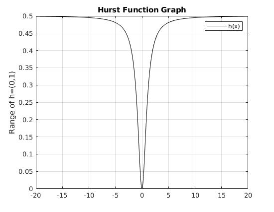
Let $h\left(x\right)=\frac{1}{2}-\frac{1/2}{1+x^{2}}\in\left(0,\frac{1}{2}\right)\subset\left(0,1\right),$ and $\left\{B_{t}\right\}_{t\in[0,T]}$ be a one-dimensional Brownian motion. Assume $X_{t}^{h}$ starts at zero and define the process as given in equation $\left(\ref{eq:SEM}\right)$ . Figure $\left(\ref{plot: SEM_ProcessEX2}\right)$ shows the plot of $h$ on the left hand side and a sample path of the process, on the right hand side, resulting from the implementation of the EM-approximation given by equation $\left(\ref{eq:EM_1}\right)$ . Is interesting noticing in this case, contrary to the previous example, that we have a rougher process than a Brownian motion at the origin, temporarily resembles the classical Brownian motion as the sample path departs from zero and gets rougher again whenever the process crosses the $x$ -axis. This makes the process go away from zero even faster due to the increased roughness.

Let $h\left(x\right)=\frac{1}{1+x^{2}}\in\left(0,1\right),$ and $\left\{B_{t}\right\}_{t\in[0,T]}$ be a one-dimensional Brownian motion. Assume $X_{t}^{h}$ starts at zero and define the process as given in equation $\left(\ref{eq:SEM}\right)$ . Figure $\left(\ref{plot: SEM_ProcesEX3}\right)$ shows the plot of $h$ on the left hand side and a sample path of the process, on the right hand side, resulting from the implementation ²² 2 All simulations were run with a step-size $\Delta t=1/100$ . of the EM-approximation given by equation $\left(\ref{eq:EM_1}\right)$ . Notice the fact that the Hurst function collapses to zero as the process departs from zero, making the process be the roughest possible. Therefore we would only recover smoother values, in particular $h=1$ only the time the sample path crossed the $x$ -axis again.

5. Self-Exciting Multifractional Gamma Processes

Barndorff-Nielsen in [1], introduces a class of self-exciting gamma type of process, in order to model turbulence, because it captures the intermittency effect observed in turbulent data. We would also like to extend our process in order to capture the previously mentioned intermittency effect. One could believe that if we were to choose a trigonometric function as a Hurst function, i.e. $h\left(t,x\right)=\alpha+\beta\cdot\sin\left(\gamma x\right),$ for some $\alpha,\beta,\gamma\in\mathbb{R}$ in the SEM process, then we might observe a regime switch in the Hurst parameters. Since the values of the process $X_{t}$ may get very large, the oscillations may take place more and more frequently. By introducing a type of gamma process (SEM-Gamma) we dampen the Volterra kernel in (1.2) by an exponential function and make the process oscillate around a mean value obtaining a more stable intermittency effect in the Hurst function.

Definition 14.

We say that a function $f:\left[0,T\right]\times\mathbb{R}\rightarrow\mathbb{R}_{+}$ is a dampening function if it is nonnegative, satisfies the following Lipschitz conditions for all $x,y\in\mathbb{R}$ and $t,t^{\prime}\in\left[0,T\right]$

\left|f\left(t,x\right)-f\left(t,y\right)\right|\leq C\left|x-y\right|,

\left|f\left(t,x\right)-f\left(t^{\prime},x\right)\right|\leq C\left|t-t^{\prime}\right|,

and satisfies the following linear growth condition for all $x\in\mathbb{R}$ and $t\in\left[0,T\right]$

\left|f\left(t,x\right)\right|\leq C\left(1+\left|x\right|\right),

for some constant $C>0$ .

Let $f$ be a dampening function and let $h$ be a Hurst function with parameters $\left(h_{*},h^{*}\right)$ . The self-excited multifractional gamma process is given formally by the Volterra equation

(5.1)

X_{t}^{h,f}=\int_{0}^{t}\exp\left(-f\left(t,X_{s}^{h,f}\right)\left(t-s\right)\right)\left(t-s\right)^{h(t,X_{s}^{h,f})-\frac{1}{2}}dB_{s}.

The following lemma shows the existence and uniqueness of the above equation by means of Theorem 2.

Lemma 15.

(5.2)

\left|\sigma\left(t,s,x\right)\right|^{2}\leq k\left(t,s\right)\left(1+\left|x\right|^{2}\right),

where

k\left(t,s\right)=C_{T}\left(t-s\right)^{2h_{*}-1},

and

(5.3)

\left|\sigma\left(t,s,x\right)-\sigma\left(t,s,y\right)\right|^{2}\leq C_{T}k\left(t,s\right)\left|\log\left(t-s\right)\right|^{2}\left|x-y\right|^{2}.

Moreover, $\sigma$ satisfies $\mathbf{H1}$ - $\mathbf{H2}$ .

Proofs for all the results in this section are reported in the appendix, since they are analogous to the ones provided previously for the SEM process.

Now since the new $\sigma$ proposed for the SEM-Gamma process also satisfies $\mathbf{H1}$ - $\mathbf{H2}$ we can apply again Zhang’s theorem, in the same way we did in Theorem 5, yielding the existence and uniqueness and bounds on $p$ -moments for the solution of

(5.4)

X_{t}^{h,f}=g\left(t\right)+\int_{0}^{t}e^{-f\left(t,X_{t}^{h,f}\right)\left(t-s\right)}\left(t-s\right)^{h\left(t,X_{t}^{h,f}\right)-\frac{1}{2}}dB_{s}.

We call this process a Self-Exciting Multifractional Gamma process (SEM-Gamma).

The following Lemma is key to study the Hölder regularity for the solution of $\left(\ref{eq: SEM-Gammaequation}\right)$ , which coincides and can be derived in the same way as for the SEM process. It is also useful for the discussion of the strong convergence of the approximating scheme given in Theorem $\left(\ref{thm:EM_StrongConvergenceGamma}\right).$

Lemma 16.

Let $\sigma(t,s,x)=\exp\left(-f\left(t,x\right)\left(t-s\right)\right)\left(t-s\right)^{h(t,x)-\frac{1}{2}}$ , such that $f$ is a dampening function and $h$ is a Hurst function with parameters $\left(h_{*},h^{*}\right)$ . Then, for any $0<\gamma<2h_{*}$ there exists $\lambda_{\gamma}:\triangle^{(3)}\left(\left[0,T\right]\right)\rightarrow\mathbb{R}$ such that

(5.5)

\left|\sigma\left(t,s,x\right)-\sigma\left(t^{\prime},s,x\right)\right|^{2}\leq\lambda_{\gamma}\left(t,t^{\prime},s\right)\left(1+\left|x\right|^{2}\right),

and

(5.6)

\int_{0}^{t^{\prime}}\lambda_{\gamma}\left(t,t^{\prime},s\right)ds\leq C_{T,\gamma}\left|t-t^{\prime}\right|^{\gamma},

for some constant $C_{T,\gamma}>0.$

In order to simulate this process we will use, again, the Euler-Maruyama approximation to discretize the continuous equation $\left(\ref{eq: SEMP_OU-Process}\right)$ . Consider a time discretization of the interval $\left[0,T\right],$ using a step-size $\Delta t=\frac{T}{N}>0$ . The EM method yields a discrete time approximation $\bar{X}_{k}^{h,f}$ of the process $X_{t_{k}}^{h,f}$ for $t_{k}=k\Delta t$ with $k\in\left\{0,\ldots,N\right\}.$ Therefore we have the following discrete time equation

(5.7)		$\displaystyle\bar{X}_{0}^{h,f}$	$\displaystyle=X_{0}^{h,f}=0$
(5.8)		$\displaystyle\bar{X}_{k}^{h,f}$	$\displaystyle=\sum_{i=0}^{k-1}\exp\left(-f\left(t_{k},\bar{X}_{i}^{h,f}\right)\left(t_{k}-t_{i}\right)\right)\left(t_{k}-t_{i}\right)^{h\left(t_{k},\bar{X}_{i}^{h,f}\right)-\frac{1}{2}}\Delta B_{i}\quad\forall k\in\left\{1,\ldots,N\right\},$

where $\Delta B_{i}=B\left(t_{i+1}\right)-B\left(t_{i}\right)$ .

Before trying to implement this approximation, in order to study the process numerically we will have to prove the following theorem to ensure the approximation is strongly converging to the process itself. It will be convenient, just as we did with the SEM process, to consider a continuous time interpolation of $\left\{\bar{X}_{k}^{h,f}\right\}_{k\in\left\{0,\ldots,N\right\}}$ given by

(5.9)

\bar{X}_{t}^{h,f}=\int_{0}^{t}\exp\left(-f\left(t,\bar{X}_{\eta\left(s\right)}^{h,f}\right)\left(t-\eta\left(s\right)\right)\right)\left(t-\eta\left(s\right)\right)^{h\left(t,\bar{X}_{\eta\left(s\right)}^{h,f}\right)-\frac{1}{2}}dB_{s},\quad\forall t\in\left[0,T\right],

where, again, $\eta\left(s\right):=t_{i}\cdot\boldsymbol{1}_{\left[t_{i},t_{i+1}\right)}\left(s\right)$ . We also have the following technical result.

Lemma 17.

Let $f$ be a dampening function, $h$ be a Hurst function with parameters $\left(h_{*},h^{*}\right)$ and $\bar{X}^{h,f}=\left\{\bar{X}_{t}^{h,f}\right\}_{t\in\left[0,T\right]}$ be given by $\left(\ref{eq:DefContEulerGamma}\right)$ . Then

(5.10)

\mathbb{E}\left[\left|\bar{X}_{t}^{h,f}\right|^{2}\right]\leq C_{T},\quad 0\leq t\leq T,

and

(5.11)

\mathbb{E}\left[\left|\bar{X}_{t}^{h,f}-\bar{X}_{t^{\prime}}^{h,f}\right|^{2}\right]\leq C_{T,\gamma}\left|t-t^{\prime}\right|^{\gamma},\quad 0\leq t^{\prime}\leq t\leq T,

for any $\gamma<2h_{*}$ , where $C_{T}$ and $C_{T,\gamma}$ are positive constants.

Using Lemma 17 and Theorem 12 we can show the order of convergence for the approximating scheme.

Theorem 18.

(5.12)

\sup_{0\leq t\leq T}\mathbb{E}\left[\left|X_{t}^{h,f}-\bar{X}_{t}^{h,f}\right|^{2}\right]\leq C_{T,\gamma,h_{*}}E_{h_{*}}\left(C_{T,\gamma,h_{*}}\Gamma\left(h_{*}\right)T^{h_{*}}\right)\left|\Delta t\right|^{\gamma},

where $\gamma\in\left(0,2h_{*}\right)$ and $C_{T,\gamma,h_{*}}$ is a positive constant, which does not depend on $N$ .

Example 19.

We will continue the previous example (4.2). In [13], D. Sornette and V. Filimonov suggested a class of self-excited processes that may exhibit all stylized facts found in financial time series as heavy tails (asset return distribution displays heavy tails with positive excess kurtosis), absence of autocorrelations (autocorrelations in asset returns are negligible, except for very short time scales $\simeq 20$ minutes), volatility clustering (absolute returns display a positive, significant and slowly decaying autocorrelation function) and the leverage effect (volatility measures of an asset are negatively correlated with its returns) among others stated in [7]. As we will see, the SEM-Gamma process resembles this properties for some choices of $h$ . The SEM-Gamma process could also be interesting for modeling commodity markets given that it mean reversion property, clustering in its increments and also stationary increments, given by the dampening through the exponential function. The right plot in Figure $\left(\ref{plot: SEM-Gamma}\right)$ , corresponds to a simulation of a sample path of the process (5.8), given the Hurst function $h$ is the same as in example (4.2) given by $h\left(x\right)=\frac{1}{1+x^{2}}$ . Notice also we have taken in this first example of the SEM-Gamma process $f\left(x\right)=0,$ which provides the regular SEM process of the previous section just to show the left plot looks very similar to the left plot in Figure $\left(\ref{plot: SEM_ProcesEX3}\right)$ .

Figure $\left(\ref{plot: SEM-Gamma_Comparative}\right)$ shows the change in the behavior of the Hurst exponent (a transition from rougher values to smoother values, i.e. $h\approx 0$ to $h\approx 1$ ) as we shift from lower values for speed of mean reversion, i.e. $f$ , to higher values. In particular we compare $f\in\left\{0,0.5,1,10\right\}$

Remark 20.

Notice one can control the clustering effect of the increments and the varying regularity of the process by controlling the parameter $f$ , regardless of the Hurst function chosen as $h$ . This is desirable in numerous fields, for example in financial markets modeling, when trying to capture shocks in asset prices. It is also important to remark the fact that using $f\left(x\right)=5,$ we reduced the amount of spikes to none, shifting the process nature from very rough and big drift, to a very smooth and driftless process. The following Figure $\left(\ref{plot: scale comparison}\right)$ shows how by zooming in the case $f\left(x\right)=5$ close enough we observe the rough nature hidden at a lower scale.

It also makes sense to let $f\left(x\right)$ be a function of $x$ , rather than a constant and in particular, if we take $f\left(x\right)=h\left(x\right)=\frac{1}{1+x^{2}}$ , we can see in the following Figure $\left(\ref{plot: SEM-Gamma h1equalh2}\right)$ how the regime switch in the Hurst exponent is less abrupt favoring sustained difference of roughness in time.

Remark 21.

The plots in Figure $\left(\ref{plot: ACF}\right)$ show the autocorrelation function of the absolute value in the time series of the increments in the SEM process (left graph) from example (4.2) and in the SEM-Gamma process (right graph) with $f\left(x\right)=0.1$ . Notice that autocorrelation in the second case is clearly much higher.

6. Appendix

In this appendix we have placed the proofs for the results related with SEM-Gamma process since they are analogous to the proofs in previous sections.

6.1. Proof of Lemma 15

Proof.

We will again proof the three results stated in the lemma by reducing them to the case proved in Lemma 4. To do so we start by proving equation $\left(\ref{eq:sigma linear growth-gamma}\right)$ . By definition, we have that

\displaystyle\sigma\left(t,s,x\right)

\displaystyle=\exp\left(-f\left(t,x\right)\left(t-s\right)\right)\left(t-s\right)^{h\left(t,x\right)-\frac{1}{2}}.

Note that

\exp\left(-f\left(t,x\right)\left(t-s\right)\right)\leq 1,

since $f\geq 0$ and $s<t$ , for all $\left(t,s\right)\in\triangle^{\left(2\right)}\left(\left[0,T\right]\right)$ . We also have that $h\left(t,x\right)\in\left[h_{*},h^{*}\right]\subset\left(0,1\right)$ for all $\left(t,x\right)\in\left[0,T\right]\times\mathbb{R}$ . Therefore the result trivially follows from Lemma 4.

Next we consider equation $\left(\ref{eq:Lipschitz sigma-gamma}\right)$ , using the fact that we can rewrite $\sigma\left(t,s,x\right)$ as

\sigma\left(t,s,x\right)=\exp\left(-f\left(t,x\right)\left(t-s\right)+\log\left(t-s\right)\left(h\left(t,x\right)-\frac{1}{2}\right)\right),

and make use again of inequality $\left(\ref{eq: expinequality}\right)$ , for all $x,y\in\mathbb{R}.$ Now we can write the following upper bound

		$\displaystyle\left\|\sigma\left(t,s,x\right)-\sigma\left(t,s,y\right)\right\|$
		$\displaystyle\leq\exp\left(\max\left(-f\left(t,x\right),-f\left(t,y\right)\right)\left(t-s\right)\right)\exp\left(\left(\max\left(h\left(t,x\right),h\left(t,y\right)\right)-\frac{1}{2}\right)\cdot\log\left(t-s\right)\right)$
		$\displaystyle\quad\times\left(\left\|f\left(t,x\right)-f\left(t,y\right)\right\|\left\|t-s\right\|+\left\|\log\left(t-s\right)\right\|\left\|h\left(t,x\right)-h\left(t,y\right)\right\|\right).$

Recalling that $\left|e^{-f\left(t,x\right)\left(t-s\right)}\right|\leq 1$ and that $f$ and $h$ are uniformly Lipschitz, we have that

		$\displaystyle\left\|\sigma\left(t,s,x\right)-\sigma\left(t,s,y\right)\right\|^{2}$
		$\displaystyle\leq C^{2}\exp\left(\max\left(\log\left(t-s\right)\left(2h\left(t,x\right)-1\right),\log\left(t-s\right)\left(2h\left(t,y\right)-1\right)\right)\right)$
		$\displaystyle\quad\times\left\|\log\left(t-s\right)\right\|^{2}\left\|x-y\right\|^{2}.$

This reduces the proof to the previous case of a SEM process, see Lemma 4. ∎

6.2. Proof of Lemma 16

Proof.

In order to prove equation $\left(\ref{eq:time reg sigma-gamma}\right)$ , it is clear that

\displaystyle\sigma\left(t,s,x\right)-\sigma\left(t^{\prime},s,x\right)

\displaystyle=e^{-f\left(t,x\right)\left(t-s\right)}\left(t-s\right)^{h\left(t,x\right)-\frac{1}{2}}-e^{-f\left(t^{\prime},x\right)\left(t^{\prime}-s\right)}\left(t^{\prime}-s\right)^{h\left(t^{\prime},x\right)-\frac{1}{2}}.

Furthermore, notice that for all $t>t^{\prime}>s>0,$ we can add and subtract the term

e^{-f\left(t,x\right)\left(t-s\right)}\left(t-s\right)^{h(t^{\prime},x)-\frac{1}{2}},

to get

\sigma\left(t,s,x\right)-\sigma\left(t^{\prime},s,x\right)=\tilde{J}^{1}\left(t,t^{\prime},s,x\right)+\tilde{J}^{2}\left(t,t^{\prime},s,x\right),

where

	$\displaystyle\tilde{J}^{1}\left(t,t^{\prime},s,x\right)$	$\displaystyle:=e^{-f\left(t,x\right)\left(t-s\right)}\left(\left(t-s\right)^{h\left(t,x\right)-\frac{1}{2}}-\left(t-s\right)^{h(t^{\prime},x)-\frac{1}{2}}\right),$
	$\displaystyle\tilde{J}^{2}\left(t,t^{\prime},s,x\right)$	$\displaystyle:=e^{-f\left(t,x\right)\left(t-s\right)}\left(t-s\right)^{h(t^{\prime},x)-\frac{1}{2}}-e^{-f\left(t^{\prime},x\right)\left(t^{\prime}-s\right)}\left(t^{\prime}-s\right)^{h\left(t^{\prime},x\right)-\frac{1}{2}}.$

First we bound $\tilde{J}^{1}$ by using that $e^{-f\left(t,x\right)\left(t-s\right)}\leq 1,$

\displaystyle\left|\tilde{J}^{1}\left(t,t^{\prime},s,x\right)\right|

\displaystyle\leq\left|J^{1}\left(t,t^{\prime},s,x\right)\right|\leq C_{T,\delta}\left|t-t^{\prime}\right|\left|t^{\prime}-s\right|^{h_{*}-\frac{1}{2}-\delta},

since $s<t^{\prime}<t,$ and where $J^{1}$ is the terms appearing in the proof of Lemma 7. Next, in order to bound the term $\tilde{J}^{2}$ , we add and subtract the quantity

e^{-f\left(t,x\right)\left(t-s\right)}\left(t^{\prime}-s\right)^{h\left(t^{\prime},x\right)-\frac{1}{2}},

to obtain

	$\displaystyle\left\|\tilde{J}^{2}\left(t,t^{\prime},s,x\right)\right\|$	$\displaystyle\leq\left\|e^{-f\left(t,x\right)\left(t-s\right)}\left(\left(t-s\right)^{h(t^{\prime},x)-\frac{1}{2}}-\left(t^{\prime}-s\right)^{h\left(t^{\prime},x\right)-\frac{1}{2}}\right)\right.$
		$\displaystyle\qquad\left.-\left(t^{\prime}-s\right)^{h\left(t^{\prime},x\right)-\frac{1}{2}}\left(e^{-f\left(t,x\right)\left(t-s\right)}-e^{-f\left(t^{\prime},x\right)\left(t^{\prime}-s\right)}\right)\right\|$
		$\displaystyle\leq\left\|e^{-f\left(t,x\right)\left(t-s\right)}\right\|\left\|\left(t-s\right)^{h(t^{\prime},x)-\frac{1}{2}}-\left(t^{\prime}-s\right)^{h\left(t^{\prime},x\right)-\frac{1}{2}}\right\|$
		$\displaystyle\qquad+\left\|\left(t^{\prime}-s\right)^{h\left(t^{\prime},x\right)-\frac{1}{2}}\right\|\left\|e^{-f\left(t,x\right)\left(t-s\right)}-e^{-f\left(t^{\prime},x\right)\left(t^{\prime}-s\right)}\right\|$
		$\displaystyle\leq\left\|J^{2}\left(t,t^{\prime},s,x\right)\right\|+\left\|\left(t^{\prime}-s\right)^{h\left(t^{\prime},x\right)-\frac{1}{2}}\right\|\left\|e^{-f\left(t,x\right)\left(t-s\right)}-e^{-f\left(t^{\prime},x\right)\left(t^{\prime}-s\right)}\right\|,$

where $J^{2}$ is the term appearing in the proof of Lemma 7. Using inequality $\left(\ref{eq: expinequality}\right)$ we can rewrite the previous expression as

	$\displaystyle\left\|\tilde{J}^{2}\left(t,t^{\prime},s,x\right)\right\|$	$\displaystyle\leq\left\|J^{2}\left(t,t^{\prime},s,x\right)\right\|+\left\|\left(t^{\prime}-s\right)^{h\left(t^{\prime},x\right)-\frac{1}{2}}\right\|$
		$\displaystyle\qquad\times\left\|e^{\max\left(-f\left(t,x\right)\left(t-s\right),-f\left(t^{\prime},x\right)\left(t^{\prime}-s\right)\right)}\right\|\left\|f\left(t^{\prime},x\right)\left(t^{\prime}-s\right)-f\left(t,x\right)\left(t-s\right)\right\|$
		$\displaystyle\leq\left\|J^{2}\left(t,t^{\prime},s,x\right)\right\|+C_{T}\left\|t^{\prime}-s\right\|^{h\left(t^{\prime},x\right)-\frac{1}{2}}\left\|t-t^{\prime}\right\|\left\|f\left(t^{\prime},x\right)-f\left(t,x\right)\right\|.$

Then, adding and subtracting $f\left(t,x\right)\left(t^{\prime}-s\right)$ , and using the linear growth and Lipschitz conditions on $f$ , we obtain

	$\displaystyle\left\|f\left(t^{\prime},x\right)\left(t^{\prime}-s\right)-f\left(t,x\right)\left(t-s\right)\right\|$	$\displaystyle\leq\left\|f\left(t,x\right)\right\|\left\|t^{\prime}-t\right\|+\left\|t^{\prime}-s\right\|\left\|f\left(t^{\prime},x\right)-f\left(t,x\right)\right\|$
		$\displaystyle\leq C\left\|t^{\prime}-t\right\|\left(1+\left\|x\right\|\right)+C\left\|t^{\prime}-s\right\|\left\|t^{\prime}-t\right\|,$

and we can conclude that

	$\displaystyle\left\|\tilde{J}^{2}\left(t,t^{\prime},s,x\right)\right\|$	$\displaystyle\leq\left\|J^{2}\left(t,t^{\prime},s,x\right)\right\|+C\left\|t^{\prime}-s\right\|^{h\left(t^{\prime},x\right)-\frac{1}{2}}\left\|t-t^{\prime}\right\|\left(1+\left\|x\right\|\right)$
		$\displaystyle\leq\left\|J^{2}\left(t,t^{\prime},s,x\right)\right\|+C_{T}\left\|t^{\prime}-s\right\|^{h_{*}-\frac{1}{2}}\left\|t-t^{\prime}\right\|\left(1+\left\|x\right\|\right).$

Therefore, if we define

\lambda_{\gamma}\left(t,t^{\prime},s\right):=C_{T,\gamma}\left(t-t^{\prime}\right)^{\gamma}\left(t^{\prime}-s\right)^{-1+h_{*}-\frac{\gamma}{2}},

for $0<\gamma<2h_{*},$ and use the final bounds for $J^{1}$ and $J^{2}$ in Lemma 7, we get that

		$\displaystyle\left\|\sigma\left(t,s,x\right)-\sigma\left(t^{\prime},s,x\right)\right\|^{2}$
		$\displaystyle\leq 4\left(\left\|J^{1}\left(t,t^{\prime},s,x\right)\right\|^{2}+\left\|J^{2}\left(t,t^{\prime},s,x\right)\right\|^{2}+\left\|C_{T}\left\|t^{\prime}-s\right\|^{h_{*}-\frac{1}{2}}\left\|t-t^{\prime}\right\|\left(1+\left\|x\right\|\right)\right\|^{2}\right)$
		$\displaystyle\leq\lambda_{\gamma}\left(t,t^{\prime},s\right)\left(1+\left\|x\right\|^{2}\right),$

and

\int_{0}^{t^{\prime}}\lambda_{\gamma}\left(t,t^{\prime},s\right)ds\leq C_{T,\gamma}\left(t^{\prime}\right)^{h_{*}-\frac{\gamma}{2}}\left(t-t^{\prime}\right)^{\gamma},

which concludes the proof. ∎

6.3. Proof of Lemma 17

Proof.

Recall that $k\left(t,s\right)=C_{T}\left(t-s\right)^{2h_{*}-1}$ and, since $\eta\left(s\right)\leq s$ , we have the following inequality

(6.1)

k\left(t,\eta\left(s\right)\right)\leq k\left(t,s\right).

Using the Itô isometry, that $e^{-2f\left(t,x\right)}\leq 1$ , equation $\left(\ref{eq:BoundSigma2_No_x}\right)$ and equation (6.1), we obtain

	$\displaystyle\mathbb{E}\left[\left\|\bar{X}_{t}^{h,f}\right\|^{2}\right]$	$\displaystyle=\mathbb{E}\left[\int_{0}^{t}e^{-2f\left(t,\bar{X}_{\eta\left(s\right)}^{h,f}\right)\left(t-\eta\left(s\right)\right)}\left(t-\eta\left(s\right)\right)^{2h\left(t,\bar{X}_{\eta\left(s\right)}^{h,f}\right)-1}ds\right]$
		$\displaystyle\leq\mathbb{E}\left[\int_{0}^{t}\left(t-\eta\left(s\right)\right)^{2h\left(t,\bar{X}_{\eta\left(s\right)}^{h,f}\right)-1}ds\right]$
		$\displaystyle\leq\int_{0}^{t}k\left(t,\eta\left(s\right)\right)ds\leq\int_{0}^{t}k\left(t,s\right)ds\leq C_{T}.$

To prove the bound $\left(\ref{eq:SecondMomentTLCE}\right),$ note that

	$\displaystyle\bar{X}_{t}^{h,f}-\bar{X}_{t^{\prime}}^{h,f}$	$\displaystyle=\int_{t^{\prime}}^{t}e^{-f\left(t,\bar{X}_{\eta\left(s\right)}^{h,f}\right)\left(t-\eta\left(s\right)\right)}\left(t-\eta\left(s\right)\right)^{h\left(t,\bar{X}_{\eta\left(s\right)}^{h,f}\right)-\frac{1}{2}}dB_{s},$
		$\displaystyle\quad+\int_{0}^{t^{\prime}}\left\{e^{-f\left(t,\bar{X}_{\eta\left(s\right)}^{h,f}\right)\left(t-\eta\left(s\right)\right)}\left(t-\eta\left(s\right)\right)^{h\left(t,\bar{X}_{\eta\left(s\right)}^{h,f}\right)-\frac{1}{2}}\right.$
		$\displaystyle\qquad\qquad\left.-e^{-f\left(t^{\prime},\bar{X}_{\eta\left(s\right)}^{h,f}\right)\left(t-\eta\left(s\right)\right)}\left(t^{\prime}-\eta\left(s\right)\right)^{h\left(t^{\prime},\bar{X}_{\eta\left(s\right)}^{h,f}\right)-\frac{1}{2}}\right\}dB_{s}$
		$\displaystyle=:J_{1}+J_{2}.$

Due to the Itô isometry, that $e^{-2f\left(t,x\right)}\leq 1$ , equation $\left(\ref{eq:BoundSigma2_No_x}\right)$ and $\left(\ref{eq: Volterrabound-1}\right)$ , we obtain the bounds

	$\displaystyle\mathbb{E}\left[\left\|J_{1}\right\|^{2}\right]$	$\displaystyle=\mathbb{E}\left[\int_{t^{\prime}}^{t}e^{-2f\left(t,\bar{X}_{\eta\left(s\right)}^{h,f}\right)\left(t-\eta\left(s\right)\right)}\left(t-\eta\left(s\right)\right)^{2h\left(t,\bar{X}_{\eta\left(s\right)}^{h,f}\right)-1}ds\right]$
		$\displaystyle\leq\int_{t^{\prime}}^{t}k\left(t,\eta\left(s\right)\right)ds\leq\int_{t^{\prime}}^{t}k\left(t,s\right)ds=C_{T}\left\|t-t^{\prime}\right\|^{2h_{*}}.$

Using again the Itô isometry, equation $\left(\ref{eq:time reg sigma-gamma}\right)$ and equation $\left(\ref{eq:TimeLispchitzIntegralLambda-gamma}\right)$ we can write, for any $\gamma<2h_{*},$ that

\displaystyle\mathbb{E}\left[\left|J_{2}\right|^{2}\right]

\displaystyle\leq\int_{0}^{t^{\prime}}\lambda_{\gamma}\left(t,t^{\prime},\eta\left(s\right)\right)\left(1+\mathbb{E}\left[\left|\bar{X}_{\eta\left(s\right)}^{h,f}\right|^{2}\right]\right)ds\leq C_{T}\int_{0}^{t^{\prime}}\lambda_{\gamma}\left(t,t^{\prime},s\right)ds\leq C_{T,\gamma}\left|t-t^{\prime}\right|^{\gamma},

where in the second inequality we have used that $\lambda_{\gamma}\left(t,t^{\prime},\eta\left(s\right)\right)\leq\lambda_{\gamma}\left(t,t^{\prime},s\right)$ , because $\lambda_{\gamma}$ is essentially a negative fractional power of $(t-s)$ and $\eta\left(s\right)\leq s$ and also that $\mathbb{E}\left[\left|\bar{X}_{t}^{h,f}\right|^{2}\right]\leq C_{T}$ , $0\leq t\leq T$ , which we just have proved above. Combining the bounds for $\mathbb{E}\left[\left|J_{1}\right|^{2}\right]$ and $\mathbb{E}\left[\left|J_{2}\right|^{2}\right]$ the result follows. ∎

6.4. Proof of Theorem 18

Proof.

We will reduce the proof to the case in Theorem 9. To do so, in the same way we did, we define

\delta_{t}:=X_{t}^{h,f}-\bar{X}_{t}^{h,f},\qquad\varphi\left(t\right):=\sup_{0\leq s\leq t}\mathbb{E}\left[\left|\delta_{s}\right|^{2}\right],\quad t\in\left[0,T\right].

For any $t\in\left[0,T\right]$ , we can write

	$\displaystyle\delta_{t}$	$\displaystyle=\int_{0}^{t}\left(e^{-f\left(t,X_{s}^{h,f}\right)\left(t-s\right)}\left(t-s\right)^{h(t,X_{s}^{h,f})-\frac{1}{2}}\right.$
		$\displaystyle\qquad-\left.e^{-f\left(t,\bar{X}_{\eta\left(s\right)}^{h,f}\right)\left(t-\eta\left(s\right)\right)}\left(t-\eta\left(s\right)\right)^{h\left(t,\bar{X}_{\eta\left(s\right)}^{h,f}\right)-\frac{1}{2}}\right)dB_{s}$
		$\displaystyle=\int_{0}^{t}\left(e^{-f\left(t,X_{s}^{h,f}\right)\left(t-s\right)}\left(t-s\right)^{h(t,X_{s}^{h,f})-\frac{1}{2}}\right.$
		$\displaystyle\qquad-\left.e^{-f\left(t,X_{s}^{h,f}\right)\left(t-s\right)}\left(t-s\right)^{h\left(t,\bar{X}_{\eta\left(s\right)}^{h,f}\right)-\frac{1}{2}}\right)dB_{s}$
		$\displaystyle+\int_{0}^{t}\left(e^{-f\left(t,X_{s}^{h,f}\right)\left(t-s\right)}\left(t-s\right)^{h\left(t,\bar{X}_{\eta\left(s\right)}^{h,f}\right)-\frac{1}{2}}\right.$
		$\displaystyle\qquad-\left.e^{-f\left(t,\bar{X}_{\eta\left(s\right)}^{h,f}\right)\left(t-\eta\left(s\right)\right)}\left(t-\eta\left(s\right)\right)^{h\left(t,\bar{X}_{\eta\left(s\right)}^{h,f}\right)-\frac{1}{2}}\right)dB_{s}$
		$\displaystyle=:\tilde{I}_{1}\left(t\right)+\tilde{I}_{2}\left(t\right).$

First we bound the second moment of $\tilde{I}_{1}\left(t\right)$ in terms of a certain integral of $\varphi$ . Using the Itô isometry, equation $\left(\ref{eq:Lipschitz sigma-gamma}\right)$ and the Lipschitz property of $h$ we get

	$\displaystyle\mathbb{E}\left[\left\|\tilde{I}_{1}\left(t\right)\right\|^{2}\right]$	$\displaystyle\leq\int_{0}^{t}k\left(t,s\right)\left(\log\left(t-s\right)\right)^{2}\mathbb{E}\left[\left(h\left(t,X_{s}^{h,f}\right)-h\left(t,\bar{X}_{\eta\left(s\right)}^{h,f}\right)\right)^{2}\right]ds$
		$\displaystyle\leq C_{T,\delta}\int_{0}^{t}\left(t-s\right)^{2\left(h_{*}-\delta\right)-1}\mathbb{E}\left[\left\|X_{s}^{h,f}-\bar{X}_{\eta\left(s\right)}^{h,f}\right\|^{2}\right]ds,$

for $\delta>0,$ arbitrarily small. By the same arguments as in the proof of Theorem 9 we obtain the following bound

(6.2)

\mathbb{E}\left[\left|\tilde{I}_{1}\right|^{2}\right]\leq C_{T,h_{*}}\left\{\int_{0}^{t}\left(t-s\right)^{h_{*}-1}\varphi\left(s\right)ds+\left|\Delta t\right|^{\gamma}\right\}.

Next, we find a bound for the second moment of $\tilde{I}_{2}\left(t\right)$ . Using again the Itô isometry, equations $\left(\ref{eq:time reg sigma-gamma}\right)$ and $\left(\ref{eq:TimeLispchitzIntegralLambda-gamma}\right)$ , and Lemma 11 we can write

(6.3)

\mathbb{E}\left[\left|\tilde{I}_{2}\right|^{2}\right]\leq\int_{0}^{t}\lambda_{\gamma}\left(t+\left(s-\eta\left(s\right)\right),t,s\right)\left(1+\mathbb{E}\left[\left|\bar{X}_{\eta\left(s\right)}^{h,f}\right|^{2}\right]\right)ds\leq C_{T,\gamma}\left|\Delta t\right|^{\gamma},

for any $\gamma<2h_{*}$ , and where we have used that

\mathbb{E}\left[\left|\bar{X}_{s}^{h,f}\right|^{2}\right]\leq C_{T},\qquad 0\leq s\leq T.

Combining the inequalities $\left(\ref{eq: barI1Bound}\right)$ and $\left(\ref{eq: barI2Bound}\right)$ we obtain

\tilde{\varphi}\left(t\right)\leq C_{T,\gamma,h_{*}}\left\{\int_{0}^{t}\left(t-s\right)^{h_{*}-1}\varphi\left(s\right)ds+\left|\Delta t\right|^{\gamma}\right\}.

Using again Lemma 12 we can conclude. ∎

References

[1] Barndorff-Nielsen, O. E. (2016). Gamma kernels and bss/lss processes. In Advanced modelling in mathematical finance. vol. 189 of Springer Proc. Math. Stat. Springer, Cham pp. 41–61.
[2] Benassi, A., Jaffard, S. and Roux, D. (1997). Elliptic Gaussian random processes. Rev. Mat. Iberoamericana 13, 19–90.
[3] Bianchi, S., Pantanella, A. and Pianese, A. (2013). Modeling stock prices by multifractional Brownian motion: an improved estimation of the pointwise regularity. Quant. Finance 13, 1317–1330.
[4] Bianchi, S., Pantanella, A. and Pianese, A. (2015). Efficient markets and behavioral finance: a comprehensive multifractional model. Adv. Complex Syst. 18, 1550001, 29.
[5] Bianchi, S. and Pianese, A. (2007). Modelling stock price movements: multifractality or multifractionality? Quant. Finance 7, 301–319.
[6] Bianchi, S. and Pianese, A. (2015). Asset price modeling: from fractional to multifractional processes. In Future perspectives in risk models and finance. vol. 211 of Internat. Ser. Oper. Res. Management Sci. Springer, Cham pp. 247–285.
[7] Cont, R. and Tankov, P. (2004). Financial modelling with jump processes. Chapman & Hall/CRC Financial Mathematics Series. Chapman & Hall/CRC, Boca Raton, FL.
[8] Corlay, S., Lebovits, J. and Véhel, J. L. (2014). Multifractional stochastic volatility models. Math. Finance 24, 364–402.
[9] Hawkes, A. G. (2018). Hawkes processes and their applications to finance: a review. Quant. Finance 18, 193–198.
[10] Ioannis Karatzas, S. S. (1998). Brownian motion and stochastic calculus, second edition. Springer.
[11] Lebovits, J. and Véhel, J. L. (2014). White noise-based stochastic calculus with respect to multifractional Brownian motion. Stochastics 86, 87–124.
[12] Pianese, A., Bianchi, S. and Palazzo, A. M. (2018). Fast and unbiased estimator of the time-dependent Hurst exponent. Chaos 28, 031102, 6.
[13] Sornette, D. and Filimonov, V. (2011). Self-excited multifractal dynamics. Europhysics Letters Association.
[14] Ye, H., Gao, J. and Ding, Y. (2007). A generalized Gronwall inequality and its application to a fractional differential equation. J. Math. Anal. Appl. 328, 1075–1081.
[15] Zhang, X. (2008). Euler schemes and large deviations for stochastic Volterra equations with singular kernels. J. Differential Equations. 244, 2226–2250.
[16] Zhang, X. (2010). Stochastic Volterra equations in Banach spaces and stochastic partial differential equation. J. Funct. Anal. 258, 1361–1425.

		$\displaystyle\left\|\sigma\left(t,s,x\right)-\sigma\left(t,s,y\right)\right\|^{2}$
		$\displaystyle\leq\exp\left(2\max\left(\log\left(t-s\right)\left(h\left(t,x\right)-\frac{1}{2}\right),\log\left(t-s\right)\left(h\left(t,y\right)-\frac{1}{2}\right)\right)\right)$
		$\displaystyle\quad\times\left\|\log\left(t-s\right)\right\|^{2}\left\|h\left(t,x\right)-h\left(t,y\right)\right\|^{2}$
		$\displaystyle\leq C^{2}\exp\left(\max\left(\log\left(t-s\right)\left(2h\left(t,x\right)-1\right),\log\left(t-s\right)\left(2h\left(t,y\right)-1\right)\right)\right)$
		$\displaystyle\quad\times\left\|\log\left(t-s\right)\right\|^{2}\left\|x-y\right\|^{2}.$

	$\displaystyle\phi_{\nu}\left(t,a\right)$	$\displaystyle:=\int_{a}^{a+t}k\left(a+t,s\right)\left\|\log\left(a+t-s\right)\right\|^{2\nu}ds$
		$\displaystyle\leq C_{T}\int_{a}^{a+t}\left(a+t-s\right)^{\left(2h_{*}-1\right)}\left\|\log\left(a+t-s\right)\right\|^{2\nu}ds$
		$\displaystyle=C_{T}\int_{0}^{t}u^{2h_{*}-1}\left\|\log\left(u\right)\right\|^{2\nu}du$
		$\displaystyle\leq C_{T}C_{T,\delta}^{2\nu}\int_{0}^{t}u^{2h_{}-1-2\nu\delta}du=C_{T,\delta,\nu,h_{}}t^{2\left(h_{*}-\nu\delta\right)},$

	$\displaystyle\left\|J^{1}\left(t,t^{\prime},s,x\right)\right\|$	$\displaystyle\leq C_{T}\left\|t-t^{\prime}\right\|\left\|t-s\right\|^{h_{*}-\frac{1}{2}}\left\|\log\left(t-s\right)\right\|$
		$\displaystyle\leq C_{T,\delta}\left\|t-t^{\prime}\right\|\left\|t-s\right\|^{h_{*}-\frac{1}{2}-\delta}$
		$\displaystyle\leq C_{T,\delta}\left\|t-t^{\prime}\right\|\left\|t^{\prime}-s\right\|^{h_{*}-\frac{1}{2}-\delta},$

	$\displaystyle\left\|J^{2}\left(t,t^{\prime},s,x\right)\right\|$	$\displaystyle\leq\frac{1}{2}\left\|t-t^{\prime}\right\|^{\alpha+\beta_{2}\left(1-\alpha\right)}\left\|t^{\prime}-s\right\|^{-\beta_{2}\left(1-\alpha\right)}$
		$\displaystyle\leq\frac{1}{2}\left\|t-t^{\prime}\right\|^{\alpha+\frac{1}{2}-\varepsilon\left(1-\alpha\right)}\left\|t^{\prime}-s\right\|^{-\frac{1}{2}+\varepsilon\left(1-\alpha\right)}$
		$\displaystyle\leq\frac{1}{2}\left\|t-t^{\prime}\right\|^{h_{*}-\varepsilon}\left\|t^{\prime}-s\right\|^{-\frac{1}{2}+\frac{\varepsilon}{2}},$

	$\displaystyle\left\|\sigma\left(t,s,x\right)-\sigma\left(t^{\prime},s,x\right)\right\|^{2}$	$\displaystyle\leq 2\left(\left\|J^{1}\left(t,t^{\prime},s,x\right)\right\|^{2}+\left\|J^{2}\left(t,t^{\prime},s,x\right)\right\|^{2}\right)$
		$\displaystyle\leq 2\left(C_{T,\delta}\left\|t-t^{\prime}\right\|^{2}\left\|t^{\prime}-s\right\|^{2h_{*}-1-2\delta}\right.$
		$\displaystyle\left.\quad+C_{T}\left\|t-t^{\prime}\right\|^{2\beta_{1}}\left\|t^{\prime}-s\right\|^{2h_{}-1-2\beta_{1}}+\frac{1}{2}\left\|t-t^{\prime}\right\|^{2h_{}-2\varepsilon}\left\|t^{\prime}-s\right\|^{-1+\varepsilon}\right)$
		$\displaystyle\leq C_{T,\beta_{1}}\left\|t-t^{\prime}\right\|^{2\beta_{1}}\left\|t^{\prime}-s\right\|^{-1+h_{*}-\beta_{1}},$