跳到论文正文
W Papers独立论文阅读器 arXiv:1908.05495 论文正文 计算阅读时间 · 0%
引用这篇论文根据当前论文元数据生成,正式投稿前建议核对。


License: arXiv.org perpetual non-exclusive license
arXiv:1908.05495v2 [math.NA] 25 Jun 2020

Ensemble Kalman filter for multiscale inverse problems

Assyr Abdulle Thanks: Institute of Mathematics, École Polytechnique Fédérale de Lausanne    Giacomo Garegnani††footnotemark:    Andrea Zanoni††footnotemark:
Abstract

We present a novel algorithm based on the ensemble Kalman filter to solve inverse problems involving multiscale elliptic partial differential equations. Our method is based on numerical homogenization and finite element discretization and allows to recover a highly oscillatory tensor from measurements of the multiscale solution in a computationally inexpensive manner. The properties of the approximate solution are analysed with respect to the multiscale and discretization parameters, and a convergence result is shown to hold. A reinterpretation of the solution from a Bayesian perspective is provided, and convergence of the approximate conditional posterior distribution is proved with respect to the Wasserstein distance. A numerical experiment validates our methodology, with a particular emphasis on modelling error and computational cost.

AMS subject classifications. 62G05, 65N21, 74Q05.

Key words. Inverse problems, Multiscale modelling, Homogenization, Ensemble Kalman filter, Bayesian inference, Modelling error.

1 Introduction

In this work we consider the application of techniques derived from the Kalman filter to inverse problems involving multiscale phenomena which can be modelled by means of partial differential equations (PDEs). Inverse problems arise in many fields, such as seismography, meteorology and tomography, all physical domains with a multiscale nature. Our reference mathematical model is given by multiscale elliptic PDEs of the form

{−∇⋅(Aεu∇pε)=f, in ​Ω,pε=0, on ​∂Ω,\left\{\begin{aligned} -\nabla\cdot(A^{\varepsilon}_{u}\nabla p^{\varepsilon})&=f,\quad&&\text{ in }\Omega,\\ p^{\varepsilon}&=0,\quad&&\text{ on }\partial\Omega,\end{aligned}\right. (1)

where Ω⊂ℝd\Omega\subset\mathbb{R}^{d} is the physical domain, AuεA_{u}^{\varepsilon} is a tensor oscillating with an amplitude described by the parameter ε\varepsilon and uu is a possibly infinite-dimensional unknown which parametrizes the tensor AuεA^{\varepsilon}_{u}. We are then interested in the solution of inverse problems involving the retrieval of the parameter uu given noisy observations derived from the solution pεp^{\varepsilon}.

Multiscale inverse problems of this form have been recently introduced in [14] and analysed extensively in [2, 3]. In particular, in [2] Abdulle and Di Blasio build a coarse-graining approach to solve the inverse problem regularized with a Tikhonov technique. The main idea is replacing the computationally expensive solution of the highly-oscillating multiscale problem with an homogenized surrogate, which eliminates the fast variables and is therefore cheaper. In particular, the theory of homogenization guarantees under certain assumptions, which will be specified throughout this work, that there exists a PDE of the form

{−∇⋅(A0u∇p0)=f, in ​Ω,p0=0, on ​∂Ω,\left\{\begin{aligned} -\nabla\cdot(A^{0}_{u}\nabla p^{0})&=f,\quad&&\text{ in }\Omega,\\ p^{0}&=0,\quad&&\text{ on }\partial\Omega,\end{aligned}\right. (2)

such that the solution p0p^{0} is the weak limit of the functions pεp^{\varepsilon} in the vanishing limit for ε\varepsilon, and such that Au0A_{u}^{0} is independent of ε\varepsilon. In [2], the authors showed that employing this homogenized model to the multiscale inverse problem guarantees a good approximation to its solution if a Tikhonov regularization is employed. This framework has been successively enlarged by the same authors to the Bayesian case in [3], where the analysis involves posterior distributions arising from both the multiscale and the homogenized model. In the same work, a technique for estimating the modelling error which was developed in [6, 5] is successfully applied to multiscale inverse problems to account for the homogenization and discretization errors.

The ensemble Kalman filter (EnKF), first introduced in [10], is an algorithm which is widely employed in the engineering community for the estimation of the state of partially-observed dynamical systems whose dynamics are governed by a nonlinear agent. In particular, Kalman filters have long been used successfully in meteorology, oceanography and automation applications. In [11], Iglesias et al. propose the application of the EnKF method to obtain a point-wise solution to inverse problems involving PDEs, and an extension of their analysis giving a Bayesian interpretation of the filtering solution is presented in [17].

In this work, we present a combination of the well-established techniques of homogenization and filtering to build a novel scheme for solving multiscale inverse problems in an efficient and reliable manner. In the same spirit of [2, 3], we prove that it is possible to eliminate the fast scales from the PDE appearing in the inverse problem relying on the theory of homogenization, thus obtaining a solution which is accurate in the vanishing limit for the multiscale parameter ε\varepsilon. In our analysis, we both consider point-wise estimations as in [11] and Bayesian solutions as in [17], thus showing convergence results which are endowed with decay rates under special assumptions on the problem. Inspired by [6, 5, 3], we then consider offline and online techniques for estimating the modelling error and prove a novel result indicating the computational cost which is required for such an estimation for any given multiscale problem.

In general, the EnKF has two main advantages with respect to other approaches. First, a Bayesian interpretation of the solution to the inverse problem is obtained from the algorithm without any additional cost. The Bayesian paradigm, frequently adopted in the context of inverse problems involving PDEs, provides a full uncertainty quantification on the solution and is therefore preferable to a point-wise estimation. Secondly, the EnKF is easily parallelizable, thus allowing in practice to solve complex inverse problems faster than employing, e.g., Markov chain Monte Carlo methods.

The main contributions of this paper are:

  • •

    to introduce a new method based on filtering techniques and numerical homogenization, which is computationally efficient and easy parallelizable to solve multiscale inverse problems;

  • •

    to analyze theoretically the convergence properties of our method both from a point-wise and a Bayesian perspectives, proving the results of convergence of the EnKF scheme in the multiscale setting;

  • •

    to estimate the modelling error caused by homogenization and discretization, and prove a novel theoretical results which strengthens its value in practice.

The outline of the work is the following. In Section 2 we briefly summarize the technique of ensemble Kalman inversion, show how it can be applied to multiscale inverse problems and state our main theoretical results. In Section 3 we present the analysis of our theoretical results, and Section 4 is dedicated to the estimation of the modelling error. Finally, in Section 5 we present a series of numerical experiments which corroborate our analysis.

2 Ensemble Kalman inversion for multiscale problems

In this section, we present the ensemble Kalman inversion technique for multiscale inverse problems. First, we introduce a generic framework and illustrate how the EnKF is employed to solve an inverse problem. Then we particularize to a inverse problems involving multiscale elliptic PDEs, and we conclude this section by announcing our main theoretical results. For a more exhaustive treatment of the EnKF in a generic PDE context, we refer the reader to [11, 17].

2.1 Ensemble Kalman inversion

We first give a brief summary of the ensemble Kalman inversion for problems of the form

find ​u∈X​ given observations ​y=𝒢⁡(u)+η∈Y,\text{find }u\in X\text{ given observations }y=\mathcal{G}(u)+\eta\in Y, (3)

where XX and YY are Hilbert spaces, the operator 𝒢:X→Y\mathcal{G}\colon X\to Y is a generic forward map and the noise η\eta follows the Gaussian distribution η∼𝒩⁡(0,Γ)\eta\sim\mathcal{N}(0,\Gamma) with a symmetric positive definite covariance Γ\Gamma. Kalman filters are traditionally employed to estimate the state of a dynamical system given partial and noisy observations of its state. In order to approximate the solution of the otherwise static problem (3), it is therefore natural to introduce some artificial dynamics. Let us consider the space Z=X×YZ=X\times Y and the map Ξ:Z→Z\Xi\colon Z\to Z given by

Ξ⁡(z)=[u𝒢⁡(u)], for z=[uv]∈Z,\Xi(z)=\begin{bmatrix}u\\ \mathcal{G}(u)\end{bmatrix},\quad\text{ for }\quad z=\begin{bmatrix}u\\ v\end{bmatrix}\in Z, (4)

Given an initial value z0∈Zz_{0}\in Z, we define artificial discrete dynamics on ZZ through the recursion

zn+1=Ξ(zn),n=0,1,…z_{n+1}=\Xi(z_{n}),\quad n=0,1,\ldots (5)

The dynamics on ZZ are completed consistently with the problem (3) by the observation equation

yn+1=H​zn+1+ηn+1,y_{n+1}=Hz_{n+1}+\eta_{n+1}, (6)

where H:Z→YH\colon Z\to Y is the projection operator defined by H=[0I]H=\begin{bmatrix}0&I\end{bmatrix} and {ηn}n∈ℕ\{\eta_{n}\}_{n\in\mathbb{N}} is an i.i.d. sequence of random variables distributed identically to the noise of the inverse problem (3), i.e., ηn∼𝒩⁡(0,Γ)\eta_{n}\sim\mathcal{N}(0,\Gamma). In fact, let us remark that combining (5) and (6) one gets yn+1=𝒢⁡(un)+ηn+1y_{n+1}=\mathcal{G}(u_{n})+\eta_{n+1}, which is in law equivalent to the equality appearing in (3).

Kalman filters proceed recursively to estimate the state of dynamics of the form (5) when observations are provided by the model (6). At each time nn, the estimation is performed in two steps. First, equation (5) is employed in the so-called prediction step, and then (6) is employed to correct the prediction in the update or analysis step. In case Ξ\Xi is a linear map, both prediction and update steps admit a closed-form expression, often referred to in literature as the Kalman formulae. Conversely, in case Ξ\Xi is nonlinear, there exist no explicit solution to the estimation problem and one has to recur to an approximation such as the EnKF method, which we briefly describe here.

Given a positive integer JJ, the EnKF method proceeds by propagating and updating an ensemble {zn(j)}j=1J⊂Z\{z_{n}^{(j)}\}_{j=1}^{J}\subset Z of particles with discrete approximations of the Kalman formulae. Let 𝒜⊂X\mathcal{A}\subset X be such that dim(𝒜)≤J\dim(\mathcal{A})\leq J, and let the initial ensemble {z0(j)}j=1J\{z_{0}^{(j)}\}_{j=1}^{J} to be given by

z0(j)=[ψ(j)𝒢⁡(ψ(j))],z_{0}^{(j)}=\begin{bmatrix}\psi^{(j)}\\ \mathcal{G}(\psi^{(j)})\end{bmatrix},

where {ψ(j)}j=1J⊂𝒜\{\psi^{(j)}\}_{j=1}^{J}\subset\mathcal{A}. At each time n=0,1,…,N−1n=0,1,\ldots,N-1, and for each j=1,…,Jj=1,\ldots,J, the prediction step is simply given by

z^n+1(j)=Ξ⁡(zn(j)).\hat{z}_{n+1}^{(j)}=\Xi(z_{n}^{(j)}). (7)

In the analysis step, this partially-updated ensemble is updated given knowledge of the data yy. For better exploring the space YY, the data is randomized and each particle zn+1(j)z_{n+1}^{(j)} is compared to i.i.d. versions of the data given by yn+1(j)=y+ηn+1(j)y_{n+1}^{(j)}=y+\eta_{n+1}^{(j)}, where ηn+1(j)∼𝒩⁡(0,Γ)\eta_{n+1}^{(j)}\sim\mathcal{N}(0,\Gamma). The analysis step is then given by

zn+1(j)=z^n+1(j)+Kn+1​(yn+1(j)−H​z^n+1(j)).z_{n+1}^{(j)}=\hat{z}_{n+1}^{(j)}+K_{n+1}(y_{n+1}^{(j)}-H\hat{z}_{n+1}^{(j)}). (8)

The operator Kn+1:Y→ZK_{n+1}\colon Y\to Z, the Kalman gain, weighs the effects of dynamics and observations in this two-step procedure, and is defined as

Kn+1=Cn+1​H∗​Rn+1,Rn+1=(H​Cn+1​H∗+Γ)−1,K_{n+1}=C_{n+1}H^{*}R_{n+1},\qquad R_{n+1}=(HC_{n+1}H^{*}+\Gamma)^{-1}, (9)

where Cn+1:Z→ZC_{n+1}\colon Z\to Z is the empirical covariance of the partially-updated ensemble {z^n+1(j)}j=1J\{\hat{z}_{n+1}^{(j)}\}_{j=1}^{J}, the operator H∗:Y→ZH^{*}\colon Y\to Z is the adjoint of HH, which is given in (6), and we recall Γ\Gamma to be the covariance of the noise yy, so that Rn+1:Y→YR_{n+1}\colon Y\to Y. Intuitively, one can notice that when the ensemble’s covariance Cn+1C_{n+1} is large with respect to the noise covariance Γ\Gamma, i.e., the observation model is more precise than the dynamics, we will have zn+1(j)≈yn+1(j)z_{n+1}^{(j)}\approx y_{n+1}^{(j)}, while in the opposite case we will have zn+1(j)≈z^n+1(j)z_{n+1}^{(j)}\approx\hat{z}_{n+1}^{(j)}. A more precise definition of the operators appearing above will be given in Section 3. At the final step NN, we project the particles on the space XX and average the result to obtain the estimate

uEnKF=1J​∑j=1JH⟂​zN(j)=1J​∑j=1JuN(j),u_{\mathrm{EnKF}}=\frac{1}{J}\sum_{j=1}^{J}H^{\perp}z_{N}^{(j)}=\frac{1}{J}\sum_{j=1}^{J}u_{N}^{(j)},

where H⟂:Z→XH^{\perp}\colon Z\to X is defined by H⟂=[I0]H^{\perp}=\begin{bmatrix}I&0\end{bmatrix}. The last detail missing to fully define the EnKF is its initialization, i.e., the choice of the space 𝒜\mathcal{A} defining the initial ensemble. We assume prior knowledge is available on the parameter u∈Xu\in X and that it is summarized by a probability measure μ0\mu_{0} on XX. In this case, one can draw JJ i.i.d. samples ψ(j)\psi^{(j)} from μ0\mu_{0} and fix 𝒜=span​{ψ(j)}j=1J\mathcal{A}=\mathrm{span}\{\psi^{(j)}\}_{j=1}^{J}.

Remark 1.

The computational cost of the EnKF method is approximately equal to the number of evaluations of the forward operator, which in a PDE framework dominates with respect to the algebraic operations needed in the analysis step. Therefore, the complexity of the algorithm is 𝒪⁡(J​N)\mathcal{O}(JN). Nonetheless, let us remark that the prediction step (7) can be easily parallelized, since the forward operator is applied independently to each particle. Hence, for a reasonable number of particles (or a high number of computing units), we have that the overall cost is of order 𝒪⁡(N)\mathcal{O}(N).

As shown in [17], a slight modification of the EnKF algorithm allows to obtain with no additional cost a Bayesian solution to (3) from the evolving ensemble. Let μ0\mu_{0} be, as above, a prior probability measure on XX and let the initial ensemble {ψ(j)}j=1J\{\psi^{(j)}\}_{j=1}^{J} consist of i.i.d. samples from μ0\mu_{0}. Given a number of steps NN, let Δ=1/N\Delta=1/N be a “stepsize”. Let us modify the algorithm above by taking instead of the covariance Γ\Gamma of the noise its scaled version Δ−1​Γ\Delta^{-1}\Gamma in formula (9). Moreover, let us define the empirical measure μ^n\hat{\mu}_{n} on XX induced by the ensemble at the nn-th step, i.e.

μ^n​(d​u)=1J​∑j=1Jδun(j)​(d​u),\hat{\mu}_{n}(du)=\frac{1}{J}\sum_{j=1}^{J}\delta_{u_{n}^{(j)}}(du), (10)

where δx\delta_{x} is the Dirac mass concentrated in x∈Ux\in U. Then, it has been shown in [17] that μ^n\hat{\mu}_{n} is a good approximation of the measure μn\mu_{n} defined by

μn​(d​u)=1Zn​e−n​Δ​Φ​(u,y)​μ0​(d​u),\mu_{n}(du)=\frac{1}{Z_{n}}e^{-n\Delta\Phi(u;y)}\mu_{0}(du), (11)

where ZnZ_{n} is the normalization constant and Φ⁡(u,y)\Phi(u;y) is the least squares functional

Φ(u;y)=12‖Γ−1/2(y−𝒢(u))‖22.\Phi(u;y)=\frac{1}{2}\left\|\Gamma^{-1/2}(y-\mathcal{G}(u))\right\|_{2}^{2}.

For n=Nn=N, we have by definition N​Δ=1N\Delta=1 and the measure μ≔μN\mu\coloneqq\mu_{N} given by

μ⁡(d​u)=1Z​e−Φ⁡(u,y)​μ0​(d​u),\mu(du)=\frac{1}{Z}e^{-\Phi(u;y)}\mu_{0}(du), (12)

where ZZ is the normalization constant, is exactly the posterior measure of the parameter uu given the prior μ0\mu_{0} in the Bayesian sense (see, e.g., [18]). Summarizing, if one carefully modifies formula (9) for the Kalman gain, it is sufficient to run the EnKF method for NN steps and the empirical measure given by the particles is an approximation to the Bayesian posterior.

2.2 Multiscale ensemble Kalman inversion

In this work, we consider the application of ensemble Kalman inversion to a multiscale inverse problem of the form

find ​u∈X​ given observations ​y=𝒢ε​(u)+η∈Y,\text{find }u\in X\text{ given observations }y=\mathcal{G}^{\varepsilon}(u)+\eta\in Y, (13)

where ε>0\varepsilon>0 is the multiscale parameter, which often is ε≪1\varepsilon\ll 1, the operator 𝒢ε:X→Y\mathcal{G}^{\varepsilon}\colon X\to Y is the multiscale forward map and where, as above, η∼𝒩⁡(0,Γ)\eta\sim\mathcal{N}(0,\Gamma) for some symmetric positive definite covariance Γ\Gamma on YY. Let Ω⊂ℝd\Omega\subset\mathbb{R}^{d} be an open bounded domain and let H01​(Ω)H_{0}^{1}(\Omega) denote the space of functions v:Ω→ℝv\colon\Omega\to\mathbb{R} in L2​(Ω)L^{2}(\Omega) with first order weak derivatives in L2​(Ω)L^{2}(\Omega) and whose trace on ∂Ω\partial\Omega vanishes. We consider the forward map 𝒢ε\mathcal{G}^{\varepsilon} to be the composition 𝒢ε=𝒪∘𝒮ε\mathcal{G}^{\varepsilon}=\mathcal{O}\circ\mathcal{S}^{\varepsilon} of an observation operator 𝒪:H01​(Ω)→Y\mathcal{O}\colon H_{0}^{1}(\Omega)\to Y and a multiscale solution operator 𝒮ε:X→H01​(Ω)\mathcal{S}^{\varepsilon}\colon X\to H_{0}^{1}(\Omega). In particular, for u∈Xu\in X, the operator 𝒮ε:u↦pε∈H01​(Ω)\mathcal{S}^{\varepsilon}\colon u\mapsto p^{\varepsilon}\in H_{0}^{1}(\Omega) where pεp^{\varepsilon} is the weak solution of the elliptic PDE

{−∇⋅(Aεu∇pε)=f, in ​Ω,pε=0, on ​∂Ω,\left\{\begin{aligned} -\nabla\cdot(A^{\varepsilon}_{u}\nabla p^{\varepsilon})&=f,\quad&&\text{ in }\Omega,\\ p^{\varepsilon}&=0,\quad&&\text{ on }\partial\Omega,\end{aligned}\right. (14)

for a right-hand side f∈L2​(Ω)f\in L^{2}(\Omega). We assume that the tensor Auε:Ω→ℝd×dA^{\varepsilon}_{u}\colon\Omega\to\mathbb{R}^{d\times d} is a parametrized multiscale tensor admitting explicit scale separation between slow and fast spatial variables, i.e.,

Auε​(x)=A⁡(u⁡(x),xε),A^{\varepsilon}_{u}(x)=A\left(u(x),\frac{x}{\varepsilon}\right),

where the map (t,x)↦A⁡(t,x/ε)(t,x)\mapsto A(t,x/\varepsilon) is assumed to be known and where AA is periodic in its second argument. In other words, the unknown uu of the inverse problem (13) governs the slow-scale variations of the rapidly-oscillating tensor AuεA_{u}^{\varepsilon}.

Let us consider now the application of ensemble Kalman inversion to the inverse problem (13). Since the PDE (14) does not in general admit a closed-form solution, one has to employ a numerical approximation to evaluate the forward map 𝒢ε\mathcal{G}^{\varepsilon}. If ε\varepsilon is small and we employ the finite element method (FEM), a fine discretization is needed to resolve the smallest scale and thus evaluate the forward operator 𝒢ε\mathcal{G}^{\varepsilon}, which clearly leads to a high computational cost. Indeed, as for Remark 1, a run of the EnKF algorithm would lead to 𝒪⁡(N)\mathcal{O}(N) solutions of (14), which is indeed unfeasible.

In order to approach the multiscale problem more efficiently we recur to the theory of homogenization (see e.g. [8]), which ensures the existence of a non-oscillating homogenized tensor Au0A^{0}_{u}, such that for ε→0\varepsilon\to 0 the solution pεp^{\varepsilon} of (14) tends weakly in H01​(Ω)H_{0}^{1}(\Omega) to the solution p0p^{0} of the problem

{−∇⋅(A0u∇p0)=f, in ​Ω,p0=0, on ​∂Ω.\left\{\begin{aligned} -\nabla\cdot(A^{0}_{u}\nabla p^{0})&=f,\quad&&\text{ in }\Omega,\\ p^{0}&=0,\quad&&\text{ on }\partial\Omega.\end{aligned}\right. (15)

Hence, this homogenized problem is a good surrogate of (14) when ε≪1\varepsilon\ll 1, and its non-oscillating nature allows us to discretize it with FEM on an arbitrarily coarse mesh, whose maximum diameter is denoted by hh. Therefore, denoting by 𝒢h0:𝒪∘𝒮h0\mathcal{G}^{0}_{h}\colon\mathcal{O}\circ\mathcal{S}^{0}_{h}, where 𝒮h0:u↦ph0\mathcal{S}^{0}_{h}\colon u\mapsto p_{h}^{0}, the numerical solution of (15), we study in this paper the behavior of the EnKF when 𝒢ε\mathcal{G}^{\varepsilon} is replaced by its cheap approximation 𝒢h0\mathcal{G}^{0}_{h}. Let us denote by {un,h0,(j)}j=1J\{u_{n,h}^{0,(j)}\}_{j=1}^{J} the ensemble obtained after nn iterations of the EnKF algorithm with the forward operators 𝒢h0\mathcal{G}_{h}^{0} in the prediction step (7). With this notation, given an initial ensemble {u0,h0,(j)}j=1J\{u_{0,h}^{0,(j)}\}_{j=1}^{J}, at each step n=0,1,…,N−1n=0,1,\ldots,N-1, our algorithm proceeds as

  1. (i)

    for each un,h0,(j)u_{n,h}^{0,(j)}, compute the homogenized tensor Aun(j)0A_{u_{n}^{(j)}}^{0} and build the forward map 𝒢h0\mathcal{G}_{h}^{0},

  2. (ii)

    perform the prediction step (7) with 𝒢h0\mathcal{G}_{h}^{0} and the analyis step (8) to obtain the updated ensemble {un+1,h0,(j)}j=1J\{u_{n+1,h}^{0,(j)}\}_{j=1}^{J}.

The computation of the homogenized tensor relies as well on numerical procedures, here we use the finite element heterogeneous multiscale method (FE-HMM) [1, 4]. Let us finally remark that similar analyses have been carried on in [14, 2, 3] for different methodologies in the solution of (13).

2.3 Statement of main results

Let us first introduce some assumptions and notation which will be employed in the analysis. First, we introduce a regularity assumption on tensors which will be fulfilled by AuεA^{\varepsilon}_{u} and Au0A^{0}_{u}.

Assumption 1.

The tensor Au:Ω→ℝd×dA_{u}\colon\Omega\to\mathbb{R}^{d\times d} satisfies for all u,u1,u2∈Xu,u_{1},u_{2}\in X and ξ∈ℝd\xi\in\mathbb{R}^{d}

‖Au1−Au2‖L∞​(Ω,ℝd×d)≤M​‖u1−u2‖X,Au​ξ⋅ξ≥α0​‖ξ‖22,\left\|A_{u_{1}}-A_{u_{2}}\right\|_{L^{\infty}(\Omega;\mathbb{R}^{d\times d})}\leq M\left\|u_{1}-u_{2}\right\|_{X},\qquad A_{u}\xi\cdot\xi\geq\alpha_{0}\left\|\xi\right\|_{2}^{2}, (16)

where MM and α0\alpha_{0} are positive constants.

We now introduce a regularity assumption on the observation operator.

Assumption 2.

The observation operator 𝒪:H01​(Ω)→Y\mathcal{O}\colon H^{1}_{0}(\Omega)\to Y satisfies for all p1,p2∈H01​(Ω)p_{1},p_{2}\in H^{1}_{0}(\Omega)

‖𝒪⁡(p1)−𝒪⁡(p2)‖Y≤C𝒪​‖p1−p2‖L2​(Ω),\left\|\mathcal{O}(p_{1})-\mathcal{O}(p_{2})\right\|_{Y}\leq C_{\mathcal{O}}\left\|p_{1}-p_{2}\right\|_{L^{2}(\Omega)},

where C𝒪C_{\mathcal{O}} is a positive constant.

Note that since 𝒪\mathcal{O} is defined on H01​(Ω)⊂L2​(Ω)H^{1}_{0}(\Omega)\subset L^{2}(\Omega), Assumption 2 is stronger than Lipschitz continuity. Finally, we introduce an assumption on the algorithm which will be employed in the analysis.

Assumption 3.

All the particles in the ensemble lie at each iteration in a ball BR​(u∗)B_{R}(u^{*}) for some R>0R>0 sufficiently big, where u∗u^{*} is the true value of the unknown.

For clarity, we present the analysis the finite-dimensional setting X=ℝMX=\mathbb{R}^{M} and Y=ℝLY=\mathbb{R}^{L} but claim that it can be readily generalized to the infinite-dimensional case. For an ensemble u={u(j)}j=1Ju=\{u^{(j)}\}_{j=1}^{J} of particles in ℝM\mathbb{R}^{M}, we introduce the ensemble norm

‖u‖≔1J​∑j=1J‖u(j)‖2,\left\|u\right\|\coloneqq\frac{1}{J}\sum_{j=1}^{J}\left\|u^{(j)}\right\|_{2}, (17)

which is indeed a norm and where ‖⋅‖2\left\|\cdot\right\|_{2} is the Euclidean norm in ℝM\mathbb{R}^{M}. Moreover, given a scalar α\alpha, we define the linear combination w=u+α​vw=u+\alpha v between two ensembles uu and vv with the same number of particles JJ as {w(j)=u(j)+αv(j)}j=1J\{w^{(j)}=u^{(j)}+\alpha v^{(j)}\}_{j=1}^{J}.

We can now present the first main result of this work, in which we show the convergence of the ensemble obtained by the EnKF employing 𝒢h0\mathcal{G}^{0}_{h} to the one obtained employing the exact operator 𝒢ε\mathcal{G}^{\varepsilon} linked to the PDE (14).

Theorem 1.

Let uN,h0={uN,h0,(j)}j=1Ju_{N,h}^{0}=\{u_{N,h}^{0,(j)}\}_{j=1}^{J}, uNε={uNε,(j)}j=1Ju_{N}^{\varepsilon}=\{u_{N}^{\varepsilon,(j)}\}_{j=1}^{J} be the ensembles after NN iterations of the EnKF method with forward operators 𝒢h0\mathcal{G}^{0}_{h} and 𝒢ε\mathcal{G}^{\varepsilon} respectively. Then, if AuεA^{\varepsilon}_{u} and Au0A^{0}_{u} satisfy Assumption 1 and if Assumption 2 and Assumption 3 hold, we have

𝔼⁡[‖uNε−uN,h0‖]→0 as ​ε,h→0.\mathbb{E}\left[\left\|u_{N}^{\varepsilon}-u_{N,h}^{0}\right\|\right]\to 0\qquad\text{ as }\varepsilon,h\to 0.

In particular, if the exact solution p0p^{0} of the homogenized problem (15) is in Hq+1​(Ω)H^{q+1}(\Omega) with q≥1q\geq 1 and we employ polynomials of degree rr for the finite element basis, then

𝔼⁡[‖uNε−uN,h0‖]≤C⁡(ε+hs+1),\mathbb{E}\left[\left\|u_{N}^{\varepsilon}-u_{N,h}^{0}\right\|\right]\leq C(\varepsilon+h^{s+1}),

where s=min⁡{r,q}s=\min\{r,q\} and C>0C>0 is a constant independent of hh and ε\varepsilon.

The proof of this result is the main focus of Section 3.1. The second main theoretical result concerns the Bayesian interpretation of the EnKF methodology for inverse problems in the multiscale setting. Let μ0\mu_{0} be a prior measure on XX and the ensembles uN,h0={uN,h0,(j)}j=1Ju_{N,h}^{0}=\{u_{N,h}^{0,(j)}\}_{j=1}^{J}, uNε={uNε,(j)}j=1Ju_{N}^{\varepsilon}=\{u_{N}^{\varepsilon,(j)}\}_{j=1}^{J} resulting from the EnKF algorithms as in Theorem 1 both initialized with an i.i.d. sample from μ0\mu_{0}. We consider the discrete probability measures

με=1J​∑j=1JδuNε,(j) and μh0=1J​∑j=1JδuN,h0,(j),\mu^{\varepsilon}=\frac{1}{J}\sum_{j=1}^{J}\delta_{u_{N}^{\varepsilon,(j)}}\qquad\text{ and }\qquad\mu_{h}^{0}=\frac{1}{J}\sum_{j=1}^{J}\delta_{u_{N,h}^{0,(j)}}, (18)

i.e., the EnKF approximations of the posterior μ\mu on uu defined in (12). Our goal is providing a measure on how far the two measures are from each other with respect to ε\varepsilon and hh. Let us remark that due to the randomization of the data at each step of the EnKF algorithm, both με\mu^{\varepsilon} and μh0\mu_{h}^{0} are random probability measures. We now introduce the metric we consider for comparing the two measures.

Definition 1.

Let (Ω,𝒜,P)(\Omega,\mathcal{A},P) be a probability space. A sequence of random measures {μn}n∈ℕ\{\mu_{n}\}_{n\in\mathbb{N}} on a metric space (E,ℬ⁡(E))(E,\mathcal{B}(E)) dependent on a random variable ξ\xi on (Ω,𝒜,P)(\Omega,\mathcal{A},P) is said to weakly converge in L1​(Ω)L^{1}(\Omega) to a random measure μ\mu on the same metric space if for all bounded continuous functions f∈CB0​(E)f\in C^{0}_{B}(E) we have

𝔼ξ​[|∫Ef​d​μn−∫Ef​𝑑μ|]→0.\mathbb{E}_{\xi}\left[\left|\int_{E}f\,d\mu_{n}-\int_{E}f\,d\mu\right|\right]\to 0.

In this case we write μn⇀L1μ\mu_{n}\xrightharpoonup{L^{1}}\mu.

We can now state our second main result, whose proof is the main focus of Section 3.2.

Theorem 2.

Let the hypotheses of Theorem 1 be satisfied. Then the sequence of random measures {με−μh0}ε,h\{\mu^{\varepsilon}-\mu_{h}^{0}\}_{\varepsilon,h}, where με\mu^{\varepsilon} and μh0\mu_{h}^{0} are defined in (18), satisfies

{με−μh0}ε,h⇀L10 as ​ε,h→0.\{\mu^{\varepsilon}-\mu_{h}^{0}\}_{\varepsilon,h}\xrightharpoonup{L^{1}}0\qquad\text{ as }\varepsilon,h\to 0.
Remark 2.

It is possible to verify that in both Theorem 1 and Theorem 2 the limits with respect to ε\varepsilon and hh can be interchanged.

3 Convergence analysis

In this section we prove Theorem 1 and Theorem 2, the main results if this work. As announced above, the analysis is carried out in the finite dimensional case X=ℝMX=\mathbb{R}^{M} and Y=ℝLY=\mathbb{R}^{L}, but it can be generalized to the infinite dimensional setting. For the purpose of the analysis, we introduce on top of the forward maps 𝒢ε\mathcal{G}^{\varepsilon} and 𝒢h0\mathcal{G}^{0}_{h}, which have been introduced in Section 2.2, the operator 𝒢0=𝒪∘𝒮0\mathcal{G}^{0}=\mathcal{O}\circ\mathcal{S}^{0}, where 𝒮0:X→H01​(Ω)\mathcal{S}^{0}\colon X\to H^{1}_{0}(\Omega) is the exact solution operator associated with the homogenized PDE (15).

3.1 Convergence of the point estimate

We now focus on Theorem 1. It is clear from the desired bound that the effects of homogenization and discretization can be analysed separately. In particular, we first show the convergence of the ensemble generated employing the forward operator 𝒢ε\mathcal{G}^{\varepsilon} to the one generated employing the exact homogenized operator 𝒢0\mathcal{G}^{0} for ε→0\varepsilon\to 0. Then, in an analogous fashion, we prove the convergence of the ensemble generated with 𝒢h0\mathcal{G}^{0}_{h} to the ensemble generated employing 𝒢0\mathcal{G}^{0}. In order to introduce a compact notation, we denote by 𝒰J,M\mathcal{U}_{J,M} the set of ensembles of dimension JJ with elements in ℝM\mathbb{R}^{M} and we consider the homogenization error function e:ℝ×𝒰J,M→ℝe\colon\mathbb{R}\times\mathcal{U}_{J,M}\to\mathbb{R}, which is defined for a generic ensemble uu as

e⁡(ε,u)=1J​∑j=1J‖𝒢ε​(u(j))−𝒢0​(u(j))‖2,e(\varepsilon,u)=\frac{1}{J}\sum_{j=1}^{J}\left\|\mathcal{G}^{\varepsilon}(u^{(j)})-\mathcal{G}^{0}(u^{(j)})\right\|_{2}, (19)

and a discretization error function e~:ℝ×𝒰J,M→ℝ\tilde{e}\colon\mathbb{R}\times\mathcal{U}_{J,M}\to\mathbb{R} as

e~​(h,u)=1J​∑j=1J‖𝒢h0​(u(j))−𝒢0​(u(j))‖2.\tilde{e}(h,u)=\frac{1}{J}\sum_{j=1}^{J}\left\|\mathcal{G}^{0}_{h}(u^{(j)})-\mathcal{G}^{0}(u^{(j)})\right\|_{2}. (20)

Before proving the main theorem, we introduce some preliminary results.

Let us first consider a generic forward operator involving an elliptic PDE and show that the associated forward map is Lipschitz continuous.

Lemma 1.

Let 𝒢:ℝM→ℝL\mathcal{G}\colon\mathbb{R}^{M}\to\mathbb{R}^{L}, 𝒢=𝒪∘𝒮\mathcal{G}=\mathcal{O}\circ\mathcal{S} be a forward operator such that 𝒪:H01​(Ω)→ℝL\mathcal{O}\colon H^{1}_{0}(\Omega)\to\mathbb{R}^{L} is Lipschitz and 𝒮:ℝM→H01​(Ω)\mathcal{S}\colon\mathbb{R}^{M}\to H^{1}_{0}(\Omega), 𝒮:u↦p\mathcal{S}\colon u\mapsto p is defined by the solution of

{−∇⋅(Au∇p)=f, in ​Ω,p=0, on ​∂Ω,\left\{\begin{aligned} -\nabla\cdot({A_{u}\nabla p})&=f,&&\quad\text{ in }\Omega,\\ p&=0,&&\quad\text{ on }\partial\Omega,\end{aligned}\right. (21)

where Ω⊂ℝd\Omega\subset\mathbb{R}^{d} is an open bounded set, the right-hand side f∈L2​(Ω)f\in L^{2}(\Omega) and the tensor AuA_{u} satisfies Assumption 1. Then 𝒢\mathcal{G} is Lipschitz with a constant depending only on the Poincaré constant of Ω\Omega, on the constants MM and α\alpha appearing in Assumption 1, on the right-hand side ff and on the Lipschitz constant of the operator 𝒪\mathcal{O}.

The proof of Lemma 1 is given in the Appendix. In the following Lemma, whose proof is also given in the Appendix, we consider the homogenization error defined in (19) and shows that it vanishes in the limit ε→0\varepsilon\to 0.

Lemma 2.

Let ee be defined as (19). Under Assumption 2, we have for all u∈𝒰J,Mu\in\mathcal{U}_{J,M}

e⁡(ε,u)→0 as ​ε→0.e(\varepsilon,u)\to 0\quad\text{ as }\varepsilon\to 0.

Moreover, if the solution of the homogenized problem (15) is in H2​(Ω)H^{2}(\Omega) independently of uu, then there exists K>0K>0 independent of ε\varepsilon and uu such that

e⁡(ε,u)≤K​ε.e(\varepsilon,u)\leq K\varepsilon.

Finally, we consider the particle empirical covariances of ensembles given by the EnKF algorithm, thus proving their boundedness and Lipschitz continuity. The proof of this Lemma can be found in the Appendix.

Lemma 3.

Let Cu​p​(u)∈ℝM×LC^{up}(u)\in\mathbb{R}^{M\times L} and Cp​p​(u)∈ℝL×LC^{pp}(u)\in\mathbb{R}^{L\times L} be defined as

Cu​p​(u)=1J​∑j=1J(u(j)−u¯)​(𝒢⁡(u(j))−𝒢¯)T,Cp​p​(u)=1J​∑j=1J(𝒢⁡(u(j))−𝒢¯)​(𝒢⁡(u(j))−𝒢¯)T,C^{up}(u)=\;\frac{1}{J}\sum_{j=1}^{J}\big(u^{(j)}-\bar{u}\big)\big(\mathcal{G}(u^{(j)})-\bar{\mathcal{G}}\big)^{T},\qquad C^{pp}(u)=\;\frac{1}{J}\sum_{j=1}^{J}\big(\mathcal{G}(u^{(j)})-\bar{\mathcal{G}}\big)\big(\mathcal{G}(u^{(j)})-\bar{\mathcal{G}}\big)^{T},

where u¯∈ℝM\bar{u}\in\mathbb{R}^{M} and 𝒢¯∈ℝL\bar{\mathcal{G}}\in\mathbb{R}^{L} are the empirical averages

u¯=1J​∑j=1Ju(j),𝒢¯=1J​∑j=1J𝒢⁡(u(j)),\bar{u}=\;\frac{1}{J}\sum_{j=1}^{J}u^{(j)},\qquad\bar{\mathcal{G}}=\;\frac{1}{J}\sum_{j=1}^{J}\mathcal{G}(u^{(j)}),

and let 𝒢:ℝM→ℝL\mathcal{G}\colon\mathbb{R}^{M}\to\mathbb{R}^{L} be Lipschitz with constant C𝒢C_{\mathcal{G}}. Then, there exist four constants Ci>0C_{i}>0, i=1,…,4i=1,\ldots,4, such that

  1. (i)

    ‖Cu​p​(u)‖2≤C1\left\|C^{up}(u)\right\|_{2}\leq C_{1},

  2. (ii)

    ‖Cp​p​(u)‖2≤C2\left\|C^{pp}(u)\right\|_{2}\leq C_{2},

  3. (iii)

    ‖Cu​p​(u1)−Cu​p​(u2)‖2≤C3​‖u1−u2‖\left\|C^{up}(u_{1})-C^{up}(u_{2})\right\|_{2}\leq C_{3}\left\|u_{1}-u_{2}\right\|,

  4. (iv)

    ‖Cp​p​(u1)−Cp​p​(u2)‖2≤C4​‖u1−u2‖\left\|C^{pp}(u_{1})-C^{pp}(u_{2})\right\|_{2}\leq C_{4}\left\|u_{1}-u_{2}\right\|,

for all ensembles u,u1,u2∈𝒰J,Mu,u_{1},u_{2}\in\mathcal{U}_{J,M} which are stable in the sense of Assumption 3.

In order to clarify the exposition, we first consider the amplification the error over one step between the EnKF algorithms employing the multiscale and the homogenized forward operators respectively, which is summarized in the following lemma.

Lemma 4.

For all n=0,…,N−1n=0,\dots,N-1, let un0={un0,(j)}j=1Ju_{n}^{0}=\{u_{n}^{0,(j)}\}_{j=1}^{J},unε={unε,(j)}j=1Ju_{n}^{\varepsilon}=\{u_{n}^{\varepsilon,(j)}\}_{j=1}^{J} be the ensembles of particles at the nn-th iteration of the EnKF for the forward operators 𝒢0\mathcal{G}^{0} and 𝒢ε\mathcal{G}^{\varepsilon} respectively. Then, under Assumption 1, Assumption 2 and Assumption 3, there exist positive constants α\alpha and γ\gamma such that

𝔼⁡[‖un+1ε−un+10‖]≤α​𝔼​[‖unε−un0‖]+γ​𝔼​[e⁡(ε,un0)],\mathbb{E}\left[\left\|u_{n+1}^{\varepsilon}-u_{n+1}^{0}\right\|\right]\leq\alpha\mathbb{E}\left[\left\|u_{n}^{\varepsilon}-u_{n}^{0}\right\|\right]+\gamma\mathbb{E}\left[e(\varepsilon,u_{n}^{0})\right], (22)

where e⁡(ε,u)e(\varepsilon,u) is given in (19).

Proof.

First, due to Assumption 2 and the Poincaré inequality with constant CpC_{p} we have

‖𝒪⁡(p1)−𝒪⁡(p2)‖2≤C𝒪​‖p1−p2‖L2​(Ω)≤C𝒪​Cp​‖∇p1−∇p2‖L2​(Ω,ℝd),\left\|\mathcal{O}(p_{1})-\mathcal{O}(p_{2})\right\|_{2}\leq C_{\mathcal{O}}\left\|p_{1}-p_{2}\right\|_{L^{2}(\Omega)}\leq C_{\mathcal{O}}C_{p}\left\|\nabla p_{1}-\nabla p_{2}\right\|_{L^{2}(\Omega;\mathbb{R}^{d})},

which shows that 𝒪\mathcal{O} is Lipschitz with constant C𝒪​CpC_{\mathcal{O}}C_{p}. Therefore, applying Lemma 1, we deduce that both 𝒢0\mathcal{G}^{0} and 𝒢ε\mathcal{G}^{\varepsilon} are Lipschitz with constant C𝒢C_{\mathcal{G}} independent of ε\varepsilon. The Kalman update formulae (8) restricted to the uu variable read (see [11])

un+1ε,(j)=\displaystyle u_{n+1}^{\varepsilon,(j)}= unε,(j)+Cu​p​(unε)​(Cp​p​(unε)+Γ)−1​(yn+1−𝒢ε​(unε,(j))),\displaystyle\;u_{n}^{\varepsilon,(j)}+C^{up}(u_{n}^{\varepsilon})(C^{pp}(u_{n}^{\varepsilon})+\Gamma)^{-1}(y_{n+1}-\mathcal{G}^{\varepsilon}(u_{n}^{\varepsilon,(j)})), (23)
un+10,(j)=\displaystyle u_{n+1}^{0,(j)}= un0,(j)+Cu​p​(un0)​(Cp​p​(un0)+Γ)−1​(yn+1−𝒢0​(un0,(j))).\displaystyle\;u_{n}^{0,(j)}+C^{up}(u_{n}^{0})(C^{pp}(u_{n}^{0})+\Gamma)^{-1}(y_{n+1}-\mathcal{G}^{0}(u_{n}^{0,(j)})). (24)

Combining (23) and (24), we have

𝔼⁡[‖un+1ε−un+10‖]=1J​∑j=1J𝔼\displaystyle\mathbb{E}\left[\left\|u_{n+1}^{\varepsilon}-u_{n+1}^{0}\right\|\right]=\;\frac{1}{J}\sum_{j=1}^{J}\mathbb{E} [‖unε,(j)+Cu​p(unε)(Cp​p(unε)+Γ)−1(yn+1(j)−𝒢ε(unε,(j)))\displaystyle\left[\left\lVert u_{n}^{\varepsilon,(j)}+C^{up}(u_{n}^{\varepsilon})(C^{pp}(u_{n}^{\varepsilon})+\Gamma)^{-1}(y_{n+1}^{(j)}-\mathcal{G}^{\varepsilon}(u_{n}^{\varepsilon,(j)}))\right.\right.
−un0,(j)−Cu​p(un0)(Cp​p(un0)+Γ)−1(yn+1(j)−𝒢0(un0,(j)))‖2],\displaystyle\left.\left.-u_{n}^{0,(j)}-C^{up}(u_{n}^{0})(C^{pp}(u_{n}^{0})+\Gamma)^{-1}(y_{n+1}^{(j)}-\mathcal{G}^{0}(u_{n}^{0,(j)}))\right\rVert_{2}\right],

and using the triangle inequality we obtain

𝔼⁡[‖un+1ε−un+10‖]≤𝔼⁡[‖unε−un0‖]+S1+S2+S3,\mathbb{E}\left[\left\|u_{n+1}^{\varepsilon}-u_{n+1}^{0}\right\|\right]\leq\operatorname{\mathbb{E}}\left[\left\|u_{n}^{\varepsilon}-u_{n}^{0}\right\|\right]+S_{1}+S_{2}+S_{3}, (25)

where

S1\displaystyle S_{1} =1J​∑j=1J𝔼⁡[‖Cu​p​(unε)−Cu​p​(un0)‖2​‖(Cp​p​(unε)+Γ)−1‖2​‖yn+1(j)−𝒢ε​(unε,(j))‖2],\displaystyle=\;\frac{1}{J}\sum_{j=1}^{J}\mathbb{E}\left[\left\|C^{up}(u_{n}^{\varepsilon})-C^{up}(u_{n}^{0})\right\|_{2}\left\|(C^{pp}(u_{n}^{\varepsilon})+\Gamma)^{-1}\right\|_{2}\left\|y_{n+1}^{(j)}-\mathcal{G}^{\varepsilon}(u_{n}^{\varepsilon,(j)})\right\|_{2}\right], (26)
S2\displaystyle S_{2} =1J​∑j=1J𝔼⁡[‖Cu​p​(un0)‖2​‖(Cp​p​(unε)+Γ)−1−(Cp​p​(un0)+Γ)−1‖2​‖yn+1(j)−𝒢ε​(unε,(j))‖2],\displaystyle=\;\frac{1}{J}\sum_{j=1}^{J}\mathbb{E}\left[\left\|C^{up}(u_{n}^{0})\right\|_{2}\left\|(C^{pp}(u_{n}^{\varepsilon})+\Gamma)^{-1}-(C^{pp}(u_{n}^{0})+\Gamma)^{-1}\right\|_{2}\left\|y_{n+1}^{(j)}-\mathcal{G}^{\varepsilon}(u_{n}^{\varepsilon,(j)})\right\|_{2}\right], (27)
S3\displaystyle S_{3} =1J​∑j=1J𝔼⁡[‖Cu​p​(un0)‖2​‖(Cp​p​(un0)+Γ)−1‖2​‖𝒢0​(un0,(j))−𝒢ε​(unε,(j))‖2].\displaystyle=\;\frac{1}{J}\sum_{j=1}^{J}\mathbb{E}\left[\left\|C^{up}(u_{n}^{0})\right\|_{2}\left\|(C^{pp}(u_{n}^{0})+\Gamma)^{-1}\right\|_{2}\left\|\mathcal{G}^{0}(u_{n}^{0,(j)})-\mathcal{G}^{\varepsilon}(u_{n}^{\varepsilon,(j)})\right\|_{2}\right]. (28)

Let us introduce two useful inequalities which will be employed in the following. Given AA and BB square invertible matrices of the same size, it holds

‖A−1−B−1‖2≤‖A−1‖2​‖B−1‖2​‖A−B‖2.\left\|A^{-1}-B^{-1}\right\|_{2}\leq\left\|A^{-1}\right\|_{2}\left\|B^{-1}\right\|_{2}\left\|A-B\right\|_{2}. (29)

Moreover, if AA is positive semidefinite and BB is positive definite, it holds

‖(A+B)−1‖2≤‖B−1‖2.\left\|(A+B)^{-1}\right\|_{2}\leq\left\|B^{-1}\right\|_{2}. (30)

Let us first consider S1S_{1}. Applying Lemma 3 and (30) to the first two factors gives

S1≤C3J​∑j=1J𝔼⁡[‖unε−un0‖​‖Γ−1‖2​‖yn+1(j)−𝒢ε​(unε,(j))‖2].S_{1}\leq\frac{C_{3}}{J}\sum_{j=1}^{J}\operatorname{\mathbb{E}}\left[\left\|u_{n}^{\varepsilon}-u_{n}^{0}\right\|\left\|\Gamma^{-1}\right\|_{2}\left\|y_{n+1}^{(j)}-\mathcal{G}^{\varepsilon}(u_{n}^{\varepsilon,(j)})\right\|_{2}\right]. (31)

Moreover, since yn+1(j)=y+ηn+1(j)y_{n+1}^{(j)}=y+\eta_{n+1}^{(j)} and since y=𝒢ε​(u∗)+ηy=\mathcal{G}^{\varepsilon}(u^{*})+\eta, where u∗u^{*} is the true value of the unknown and η\eta is the true realization of the noise, the triangle inequality yields

‖yn+1(j)−𝒢ε​(unε,(j))‖2≤‖𝒢ε​(u∗)−𝒢ε​(unε,(j))‖2+‖ηn+1(j)+η‖2,\left\|y_{n+1}^{(j)}-\mathcal{G}^{\varepsilon}(u_{n}^{\varepsilon,(j)})\right\|_{2}\leq\left\|\mathcal{G}^{\varepsilon}(u^{*})-\mathcal{G}^{\varepsilon}(u_{n}^{\varepsilon,(j)})\right\|_{2}+\left\|\eta_{n+1}^{(j)}+\eta\right\|_{2}, (32)

which, since 𝒢ε\mathcal{G}^{\varepsilon} is Lipschitz and due to Assumption 3, implies

‖yn+1(j)−𝒢ε​(unε,(j))‖2≤C𝒢​R+‖ηn+1(j)+η‖2.\left\|y_{n+1}^{(j)}-\mathcal{G}^{\varepsilon}(u_{n}^{\varepsilon,(j)})\right\|_{2}\leq C_{\mathcal{G}}R+\left\|\eta_{n+1}^{(j)}+\eta\right\|_{2}. (33)

Hence, we get

S1≤1J​C3​‖Γ−1‖2​∑j=1J𝔼⁡[‖unε−un0‖​(C𝒢​R+‖ηn+1(j)+η‖2)].S_{1}\leq\frac{1}{J}C_{3}\left\|\Gamma^{-1}\right\|_{2}\sum_{j=1}^{J}\mathbb{E}\left[\left\|u_{n}^{\varepsilon}-u_{n}^{0}\right\|\left(C_{\mathcal{G}}R+\left\|\eta_{n+1}^{(j)}+\eta\right\|_{2}\right)\right].

Finally, the random variables ζn+1(j)≔ηn+1(j)+η\zeta_{n+1}^{(j)}\coloneqq\eta_{n+1}^{(j)}+\eta are i.i.d., distributed as ζ∼𝒩⁡(0,2​Γ)\zeta\sim\mathcal{N}(0,2\Gamma) and independent of unεu_{n}^{\varepsilon} and un0u_{n}^{0}, which implies first

𝔼⁡[‖ζ‖2]≤𝔼⁡[‖ζ‖22]=2​tr​(Γ),\mathbb{E}[\left\|\zeta\right\|_{2}]\leq\sqrt{\mathbb{E}[\left\|\zeta\right\|_{2}^{2}]}=\sqrt{2\mathrm{tr}(\Gamma)},

and second, defining α1≔C3​‖Γ−1‖2​(C𝒢​R+2​tr​(Γ))\alpha_{1}\coloneqq C_{3}\left\|\Gamma^{-1}\right\|_{2}(C_{\mathcal{G}}R+\sqrt{2\mathrm{tr}(\Gamma)}), yields the final bound

S1≤α1​𝔼​[‖unε−un0‖].S_{1}\leq\alpha_{1}\mathbb{E}\left[\left\|u_{n}^{\varepsilon}-u_{n}^{0}\right\|\right]. (34)

Let us now consider the second term S2S_{2}. We apply Lemma 3 to the norm of Cu​p​(un0)C^{up}(u_{n}^{0}). Moreover, applying the inequalities (29), (30) and Lemma 3 gives

‖(Cp​p​(unε)+Γ)−1−(Cp​p​(un0)+Γ)−1‖2≤C4​‖Γ−1‖22​‖unε−un0‖.\left\|(C^{pp}(u_{n}^{\varepsilon})+\Gamma)^{-1}-(C^{pp}(u_{n}^{0})+\Gamma)^{-1}\right\|_{2}\leq C_{4}\left\|\Gamma^{-1}\right\|_{2}^{2}\left\|u_{n}^{\varepsilon}-u_{n}^{0}\right\|. (35)

Reasoning as for S1S_{1} for the third factor appearing in (27) finally yields

S2≤α2​𝔼​[‖unε−un0‖],S_{2}\leq\alpha_{2}\mathbb{E}\left[\left\|u_{n}^{\varepsilon}-u_{n}^{0}\right\|\right], (36)

where α2≔C1​C4​‖Γ−1‖22​(C𝒢​R+2​tr​(Γ))\alpha_{2}\coloneqq C_{1}C_{4}\left\|\Gamma^{-1}\right\|_{2}^{2}(C_{\mathcal{G}}R+\sqrt{2\mathrm{tr}(\Gamma)}). We now consider the last term S3S_{3}. The first factor appearing in (28) can be bounded by Lemma 3 and for the second factor we use (30), thus obtaining

‖(Cp​p​(un0)+Γ)−1‖2≤‖Γ−1‖2.\left\|(C^{pp}(u_{n}^{0})+\Gamma)^{-1}\right\|_{2}\leq\left\|\Gamma^{-1}\right\|_{2}.

Regarding the third factor of (28), we apply the triangle inequality and the Lipschitz continuity of the forward operator 𝒢ε\mathcal{G}^{\varepsilon}, which yield

‖𝒢0​(un0,(j))−𝒢ε​(unε,(j))‖2≤‖𝒢0​(un0,(j))−𝒢ε​(un0,(j))‖2+C𝒢​‖un0,(j)−unε,(j)‖2.\left\|\mathcal{G}^{0}(u_{n}^{0,(j)})-\mathcal{G}^{\varepsilon}(u_{n}^{\varepsilon,(j)})\right\|_{2}\leq\left\|\mathcal{G}^{0}(u_{n}^{0,(j)})-\mathcal{G}^{\varepsilon}(u_{n}^{0,(j)})\right\|_{2}+C_{\mathcal{G}}\left\|u_{n}^{0,(j)}-u_{n}^{\varepsilon,(j)}\right\|_{2}. (37)

Substituting back into S3S_{3} and by definition of e⁡(ε,un0)e(\varepsilon,u_{n}^{0}) and of the ensemble norm we obtain

S3≤C1​‖Γ−1‖2​𝔼​[e⁡(ε,un0)]+C1​‖Γ−1‖2​C𝒢​𝔼​[‖un0−unε‖].S_{3}\leq C_{1}\left\|\Gamma^{-1}\right\|_{2}\mathbb{E}\left[e(\varepsilon,u_{n}^{0})\right]+C_{1}\left\|\Gamma^{-1}\right\|_{2}C_{\mathcal{G}}\mathbb{E}\left[\left\|u_{n}^{0}-u_{n}^{\varepsilon}\right\|\right].

Therefore, defining α3=C1​‖Γ−1‖2​C𝒢\alpha_{3}=C_{1}\left\|\Gamma^{-1}\right\|_{2}C_{\mathcal{G}} and γ=C1​‖Γ−1‖2\gamma=C_{1}\left\|\Gamma^{-1}\right\|_{2} we have the bound

S3≤α3​𝔼​[‖un0−unε‖]+γ​𝔼​[e⁡(ε,un0)].S_{3}\leq\alpha_{3}\mathbb{E}\left[\left\|u_{n}^{0}-u_{n}^{\varepsilon}\right\|\right]+\gamma\mathbb{E}\left[e(\varepsilon,u_{n}^{0})\right]. (38)

Finally, defining α≔1+α1+α2+α3\alpha\coloneqq 1+\alpha_{1}+\alpha_{2}+\alpha_{3}, and using the results (25), (34), (36) and (38), we obtain the desired result. ∎

We now present the main result about global multiscale convergence of the EnKF algorithm.

Proposition 1.

Under the notation and assumptions of Lemma 4, letting u0ε=u00u_{0}^{\varepsilon}=u_{0}^{0} be the same initial ensemble, we have

𝔼⁡[‖uNε−uN0‖]→0 as ​ε→0.\mathbb{E}\left[\left\|u_{N}^{\varepsilon}-u_{N}^{0}\right\|\right]\to 0\qquad\text{ as }\varepsilon\to 0.

Moreover, if the solution of the homogenized problem (15) is sufficiently regular, namely p0∈H2​(Ω)p^{0}\in H^{2}(\Omega), then there exists K1>0K_{1}>0 independent of ε\varepsilon such that

𝔼⁡[‖uNε−uN0‖]≤K1​ε.\mathbb{E}\left[\left\|u_{N}^{\varepsilon}-u_{N}^{0}\right\|\right]\leq K_{1}\varepsilon.
Proof.

Since u0ε=u00u_{0}^{\varepsilon}=u_{0}^{0}, iterating the estimate of Lemma 4 yields

𝔼⁡[‖uNε−uN0‖]≤γ​∑i=0N−1αN−1−i​𝔼​[e⁡(ε,ui0)].\mathbb{E}\left[\left\|u_{N}^{\varepsilon}-u_{N}^{0}\right\|\right]\leq\gamma\sum_{i=0}^{N-1}\alpha^{N-1-i}\mathbb{E}\left[e(\varepsilon,u^{0}_{i})\right].

Applying Lemma 2, we have e⁡(ε,ui0)→0e(\varepsilon,u_{i}^{0})\to 0 for all i=0,…,N−1i=0,\dots,N-1, hence as ε→0\varepsilon\to 0

𝔼⁡[‖uNε−uN0‖]→0.\mathbb{E}\left[\left\|u_{N}^{\varepsilon}-u_{N}^{0}\right\|\right]\to 0.

Moreover, if p0p^{0} belongs to H2​(Ω)H^{2}(\Omega), applying Lemma 2 gives

𝔼⁡[‖uNε−uN0‖]≤K1​ε,\mathbb{E}\left[\left\|u_{N}^{\varepsilon}-u_{N}^{0}\right\|\right]\leq K_{1}\varepsilon, (39)

where K1=γ⁡(αN−1)​K/(α−1)K_{1}=\gamma(\alpha^{N}-1)K/(\alpha-1), which is the desired result. ∎

We now consider convergence with respect to the FEM discretization of the homogenized problem. First, we introduce a preliminary result, which plays the role of Lemma 2 in the context of numerical convergence and whose proof is given in the Appendix.

Lemma 5.

Let e~\tilde{e} be defined in (20) and let Assumption 2 hold. If the exact solution p0p^{0} of the homogenized problem (21) is in Hq+1​(Ω)H^{q+1}(\Omega), the right-hand side ff is in Hq−1​(Ω)H^{q-1}(\Omega) and we employ polynomials of degree rr for the finite element basis, then

e~​(h,u)≤K~​hs+1,\tilde{e}(h,u)\leq\tilde{K}h^{s+1},

where s=min⁡{r,q}s=\min\{r,q\}.

We can now state the main result concerning convergence with respect to the numerical discretization of the homogenized problem.

Proposition 2.

Let uN0={uN0,(j)}j=1Ju_{N}^{0}=\{u_{N}^{0,(j)}\}_{j=1}^{J}, uN,h0={uN,h0,(j)}j=1Ju_{N,h}^{0}=\{u_{N,h}^{0,(j)}\}_{j=1}^{J} be the ensembles of particles at the last iteration of the iterative ensemble Kalman filter for the forward operators 𝒢0\mathcal{G}^{0} and 𝒢h0\mathcal{G}_{h}^{0} respectively. Then, under Assumption 1, Assumption 2, Assumption 3 and if the exact solution p0p^{0} of the homogenized problem (21) is in Hq+1​(Ω)H^{q+1}(\Omega) and we use polynomials of degree rr for the finite element basis, we have

𝔼⁡[‖uN,h0−uN0‖]≤K2​hs+1,\mathbb{E}\left[\left\|u_{N,h}^{0}-u_{N}^{0}\right\|\right]\leq K_{2}h^{s+1},

where s=min⁡{r,q}s=\min\{r,q\} and K2K_{2} is a positive constant independent of hh.

Proof.

The proof of Proposition 2 is identical to the proof of Proposition 1, except that all the ensembles {unε}n=1N\{u_{n}^{\varepsilon}\}_{n=1}^{N} obtained by the multiscale operator 𝒢ε\mathcal{G}^{\varepsilon} have to be replaced by the ensembles {un,h0}n=1N\{u_{n,h}^{0}\}_{n=1}^{N} obtained by the finite element discretization of the homogenized operator 𝒢h0\mathcal{G}^{0}_{h}. Moreover Lemma 2 for the error ee has to be replaced by Lemma 5 for the error e~\tilde{e}. ∎

Applying Proposition 1 and Proposition 2, we finally prove Theorem 1.

Proof of Theorem 1.

An application of the triangle inequality yields

𝔼⁡[‖uNε−uN,h0‖]≤𝔼⁡[‖uNε−uN0‖]+𝔼⁡[‖uN0−uN,h0‖].\mathbb{E}[\left\|u_{N}^{\varepsilon}-u_{N,h}^{0}\right\|]\leq\mathbb{E}[\left\|u_{N}^{\varepsilon}-u_{N}^{0}\right\|]+\mathbb{E}[\left\|u_{N}^{0}-u_{N,h}^{0}\right\|].

The two addends can be bounded applying Proposition 1 and Proposition 2, thus obtaining the desired result for C=max⁡{K1,K2}C=\max\{K_{1},K_{2}\}. ∎

3.2 Convergence of the posterior distributions

In this section, we give the proof of Theorem 2, i.e., the convergence of the discrete posterior measures με\mu^{\varepsilon} to μh0\mu^{0}_{h} introduced in (18) as ε,h→0\varepsilon,h\to 0. Let u∗∈ℝMu^{*}\in\mathbb{R}^{M} and let BR​(u∗)B_{R}(u^{*}) be the ball of radius RR centered in u∗u^{*} with respect to the norm ‖⋅‖s\left\|\cdot\right\|_{s} with s∈[1,∞]s\in[1,\infty]. Due to the discrete nature of these distributions, we study convergence with respect to the Wasserstein metrics, for which we report its standard definition in the metric spaces (BR​(u∗),‖⋅‖s)(B_{R}(u^{*}),\left\|\cdot\right\|_{s}), which can be found, e.g., in [16].

Definition 2.

Let μ\mu and ν\nu be two probability measures on the metric space (BR​(u∗),‖⋅‖s)(B_{R}(u^{*}),\left\|\cdot\right\|_{s}). The Wasserstein distance between μ\mu and ν\nu is defined for all p∈[1,∞)p\in[1,\infty) as

Wp,s​(μ,ν)=(infγ∈Γ⁡(μ,ν)∫BR​(u∗)×BR​(u∗)‖u−v‖sp​𝑑γ​(u,v))1/p,W_{p,s}(\mu,\nu)=\left(\inf_{\gamma\in\Gamma(\mu,\nu)}\int_{B_{R}(u^{*})\times B_{R}(u^{*})}\left\|u-v\right\|_{s}^{p}d\gamma(u,v)\right)^{1/p}, (40)

where Γ⁡(μ,ν)\Gamma(\mu,\nu) denotes the collection of all joint distributions on BR​(u∗)×BR​(u∗)B_{R}(u^{*})\times B_{R}(u^{*}) with marginals μ\mu and ν\nu on the first and second factors respectively.

Remark 3.

If μ\mu and ν\nu are two discrete distributions on finite state spaces, respectively Ω1={u1,…,uK1}\Omega_{1}=\{u_{1},\dots,u_{K_{1}}\} and Ω2={v1,…,vK2}\Omega_{2}=\{v_{1},\dots,v_{K_{2}}\} included in BR​(u∗)B_{R}(u^{*}), then (40) can be written as

Wp,s​(μ,ν)=(infγ∈ℝK1×K2∑i=1K1∑j=1K2‖ui−vj‖sp​γi​j)1/p,W_{p,s}(\mu,\nu)=\left(\inf_{\gamma\in\mathbb{R}^{K_{1}\times K_{2}}}\sum_{i=1}^{K_{1}}\sum_{j=1}^{K_{2}}\left\|u_{i}-v_{j}\right\|_{s}^{p}\gamma_{ij}\right)^{1/p}, (41)

where the matrix γ\gamma has to satisfy the following constraints

∑j=1K2γi​j=μ⁡(ui)for all ​i=1,…​K1,∑i=1K1γi​j=ν⁡(vj)for all ​j=1,…​K2.\sum_{j=1}^{K_{2}}\gamma_{ij}=\mu(u_{i})\quad\text{for all }i=1,\dots K_{1},\qquad\sum_{i=1}^{K_{1}}\gamma_{ij}=\nu(v_{j})\quad\text{for all }j=1,\dots K_{2}. (42)

We now show that the distance W1,2W_{1,2} is bounded by the distance induced by the ensemble norm defined in (17). This result will be crucial later to prove Theorem 1.

Lemma 6.

Let u1={u1(j)}j=1Ju_{1}=\{u_{1}^{(j)}\}_{j=1}^{J}, u2={u2(j)}j=1Ju_{2}=\{u_{2}^{(j)}\}_{j=1}^{J} be two ensembles of particles and let μ1,μ2\mu_{1},\mu_{2} be the corresponding distributions defined as sum of Dirac masses

μ1=1J​∑j=1Jδu1(j),μ2=1J​∑j=1Jδu2(j).\mu_{1}=\frac{1}{J}\sum_{j=1}^{J}\delta_{u_{1}^{(j)}},\qquad\qquad\mu_{2}=\frac{1}{J}\sum_{j=1}^{J}\delta_{u_{2}^{(j)}}.

Then for all s∈[1,∞]s\in[1,\infty] and p∈[1,∞)p\in[1,\infty) it holds

Wp,s​(μ1,μ2)≤(1J​∑j=1J‖u1(j)−u2(j)‖sp)1pW_{p,s}(\mu_{1},\mu_{2})\leq\left(\frac{1}{J}\sum_{j=1}^{J}\left\|u_{1}^{(j)}-u_{2}^{(j)}\right\|_{s}^{p}\right)^{\frac{1}{p}}

and, in particular,

W1,2​(μ1,μ2)≤‖u1−u2‖.W_{1,2}(\mu_{1},\mu_{2})\leq\left\|u_{1}-u_{2}\right\|.
Proof.

Take γ∗\gamma^{*} defined as

γ∗​(u1(j),u2(i))={1J if ​i=j0 if ​i≠j,\gamma^{*}(u_{1}^{(j)},u_{2}^{(i)})=\begin{cases}\frac{1}{J}&\text{ if }i=j\\ 0&\text{ if }i\neq j,\end{cases}

which satisfies the constraints (42), and note that

∑j=1J∑i=1J‖u1(j)−u2(i)‖sp​γ∗​(u1(j),u2(i))=1J​∑j=1J‖u1(j)−u2(j)‖sp.\sum_{j=1}^{J}\sum_{i=1}^{J}\left\|u_{1}^{(j)}-u_{2}^{(i)}\right\|_{s}^{p}\gamma^{*}(u_{1}^{(j)},u_{2}^{(i)})=\frac{1}{J}\sum_{j=1}^{J}\left\|u_{1}^{(j)}-u_{2}^{(j)}\right\|_{s}^{p}.

Therefore, by definition of Wasserstein distance for discrete distributions on finite spaces (41), we deduce that

Wp,s​(μ1,μ2)≤(1J​∑j=1J‖u1(j)−u2(j)‖sp)1p,W_{p,s}(\mu_{1},\mu_{2})\leq\left(\frac{1}{J}\sum_{j=1}^{J}\left\|u_{1}^{(j)}-u_{2}^{(j)}\right\|_{s}^{p}\right)^{\frac{1}{p}},

which is the desired result. Finally, taking p=1p=1 and s=2s=2 and recalling the ensemble norm defined in (17), we obtain the second inequality. ∎

We now analyze the relationship between the weak L1L^{1} convergence introduce in Definition 1 and the convergence with respect to the expectation of the Wasserstein distance for random probability measures. In particular, we prove that the latter implies the former, which was already proved in [16] for non-random measures. Here, we extend the result to random probability measures. The proof of the following Lemma is given in the Appendix.

Lemma 7.

Let (Ω,𝒜,P)(\Omega,\mathcal{A},P) be a probability space. Let the sequence {μn}n∈ℕ\{\mu_{n}\}_{n\in\mathbb{N}} and μ\mu be random probability measures on the metric space (BR​(u∗),‖⋅‖s)(B_{R}(u^{*}),\left\|\cdot\right\|_{s}) dependent on the random variable ξ\xi on (Ω,𝒜,P)(\Omega,\mathcal{A},P). If

𝔼ξ​[W1,s​(μn,μ)]→0,\mathbb{E}_{\xi}[W_{1,s}(\mu_{n},\mu)]\to 0,

then μn⇀L1μ\mu_{n}\xrightharpoonup{L^{1}}\mu.

We can now complete the proof of Theorem 2.

Proof of Theorem 2.

Applying Lemma 6 and due to Theorem 1, we deduce that for ε,h→0\varepsilon,h\to 0 it holds

𝔼⁡[W1,2​(με,μh0)]→0.\mathbb{E}[W_{1,2}(\mu^{\varepsilon},\mu_{h}^{0})]\to 0.

Note that the only difference in the update step of the EnKF when used for a point estimate and in the Bayesian framework is that Γ\Gamma is replaced by Δ−1​Γ\Delta^{-1}\Gamma where Δ=1/N\Delta=1/N. The constants of the proof of Theorem 1 depend on ‖Γ−1‖2\left\|\Gamma^{-1}\right\|_{2}, which is now replaced by ‖(Δ−1​Γ)−1‖2\left\|(\Delta^{-1}\Gamma)^{-1}\right\|_{2}, which can be bounded by ‖Γ−1‖2\left\|\Gamma^{-1}\right\|_{2} as

‖(Δ−1​Γ)−1‖2=Δ​‖Γ−1‖2≤‖Γ−1‖2.\left\|(\Delta^{-1}\Gamma)^{-1}\right\|_{2}=\Delta\left\|\Gamma^{-1}\right\|_{2}\leq\left\|\Gamma^{-1}\right\|_{2}.

Finally, applying Lemma 7, we obtain the desired result. ∎

4 Modelling error

In this section, we consider the effects of model misspecification due to the homogenization and discretization error. All the results presented in Section 3 deal with the asymptotic case h,ε→0h,\varepsilon\to 0, which is unrealistic in applications. Let us recall that the original inverse problem involves predicting the exact unknown u∗u^{*} from observations originated by the model

y=𝒢ε​(u∗)+η,y=\mathcal{G}^{\varepsilon}(u^{*})+\eta, (43)

where η∼𝒩⁡(0,Γ)\eta\sim\mathcal{N}(0,\Gamma) is the noise. Since evaluating 𝒢ε\mathcal{G}^{\varepsilon} is too expensive and in many applications unfeasible, we wish to employ the cheaper forward operator 𝒢h0\mathcal{G}^{0}_{h}. Hence, we rewrite (43) as

y=𝒢h0​(u∗)+ℰ⁡(u∗)+η,y=\mathcal{G}^{0}_{h}(u^{*})+\mathcal{E}(u^{*})+\eta, (44)

where

ℰ⁡(u∗)≔𝒢ε​(u∗)−𝒢h0​(u∗).\mathcal{E}(u^{*})\coloneqq\mathcal{G}^{\varepsilon}(u^{*})-\mathcal{G}^{0}_{h}(u^{*}).

The quantity ℰ⁡(u∗)\mathcal{E}(u^{*}) represents the error introduced by misspecification of the forward model. Equation (44) shows that the observed data yy can be seen as data originating by the discrete homogenized model which is affected by two sources of errors, the original noise and the modelling error. This formulation of modelling error was originally presented in [6], and then applied to multiscale inverse problems in [3]. Following [6, 3], we assume that the modelling error is a Gaussian random variable independent of the noise η\eta, so that ℰ∼𝒩⁡(m,Σ)\mathcal{E}\sim\mathcal{N}(m,\Sigma) for all uu, and write

y=𝒢h0​(u∗)+m+ζ+η,y=\mathcal{G}^{0}_{h}(u^{*})+m+\zeta+\eta, (45)

where ζ∼𝒩⁡(0,Σ)\zeta\sim\mathcal{N}(0,\Sigma). There is no theoretical guarantee for the modelling error to be distributed as a Gaussian in this framework. Nevertheless, it has been shown in [13] that in the one-dimensional case a Gaussian assumption can be employed effectively for the modelling error, thus partially justifying our choice. Then we define

y~=y−mandη~=η+ζ∼𝒩⁡(0,Γ+Σ)\tilde{y}=y-m\qquad\text{and}\qquad\tilde{\eta}=\eta+\zeta\sim\mathcal{N}(0,\Gamma+\Sigma)

and, from (45), we obtain

y~=𝒢h0​(u∗)+η~.\tilde{y}=\mathcal{G}^{0}_{h}(u^{*})+\tilde{\eta}. (46)

Therefore, if the mean mm and covariance Σ\Sigma of the modelling error are known, a more reliable approximation of the unknown u∗u^{*} can be obtained applying the EnKF to (46). The modelling error distribution, by assumption fully determined by its mean and covariance, is approximated offline. We sample NℰN_{\mathcal{E}} unknowns {ui}i=1Nℰ\{u_{i}\}_{i=1}^{N_{\mathcal{E}}} from μ0\mu_{0} and, for all i=1,…,Nℰi=1,\dots,N_{\mathcal{E}}, we apply both the forward operators 𝒢ε​(ui)\mathcal{G}^{\varepsilon}(u_{i}) and 𝒢h0​(ui)\mathcal{G}^{0}_{h}(u_{i}). Then we compute

ℰi=𝒢ε​(ui)−𝒢h0​(ui),\mathcal{E}_{i}=\mathcal{G}^{\varepsilon}(u_{i})-\mathcal{G}^{0}_{h}(u_{i}),

and the mean mm and the covariance Σ\Sigma are obtained as the empirical mean and covariance of the sample {ℰi}i=1Nℰ\{\mathcal{E}_{i}\}_{i=1}^{N_{\mathcal{E}}}. This procedure is computationally involved due to the multiple evaluations of 𝒢ε\mathcal{G}^{\varepsilon}, but it has to be performed only once and can then be applied to different sets of observations and true values u∗u^{*}. Let us also remark that on the one hand, due to the theory of homogenization, the modelling error can be considered negligible when ε\varepsilon is very small, and the expensive estimation of ℰ\mathcal{E} may not be necessary. On the other hand, when ε\varepsilon is larger, the homogenized equation does not provide with a good approximation of the multiscale problem, and an estimation of ℰ\mathcal{E} is required. One may rightfully argue that in case ε=𝒪⁡(1)\varepsilon=\mathcal{O}(1), it is possible to evaluate the forward operator 𝒢ε\mathcal{G}^{\varepsilon} without a large computational effort. Hence, the techniques presented in this section are relevant for mid-range values of ε\varepsilon, for which ℰ\mathcal{E} is significant with respect to the noise η\eta. Moreover, we remarked in practice via numerical experiments that a small number NℰN_{\mathcal{E}} can be employed to obtain a satisfactory approximation of the modelling error. A theoretical justification of this property is provided by Theorem 3 and Theorem 4.

In order to obtain a more reliable approximation of the distribution of the modelling error, we can follow a dynamic approach based on the estimation of the mean mm and the covariance Σ\Sigma online, i.e., during the run of the EnKF algorithm. This methodology has been developed in [5]. In particular, we sequentially apply the ensemble Kalman method for ℒ\mathcal{L} levels and, at each level ℓ=1,…,ℒ\ell=1,\dots,\mathcal{L}, we update the distribution of the modelling error, which is denoted by νℓ=𝒩⁡(mℓ,Σℓ)\nu^{\ell}=\mathcal{N}(m^{\ell},\Sigma^{\ell}). Letting

μnℓ=1J​∑j=1Jδunℓ⁡(j)\mu_{n}^{\ell}=\frac{1}{J}\sum_{j=1}^{J}\delta_{u^{\ell(j)}_{n}}

be the approximation of the distribution of the particles at iteration nn at level ℓ\ell, μ0ℓ+1=μNℓℓ\mu_{0}^{\ell+1}=\mu_{N^{\ell}}^{\ell} and μ01=μ0\mu_{0}^{1}=\mu_{0}, where NℓN^{\ell} is the number of iterations at level ℓ\ell, then the mean mℓm^{\ell} and the covariance Σℓ\Sigma^{\ell} are approximated as in the offline approach with the only difference that μ0\mu_{0} is replaced by μ0ℓ\mu_{0}^{\ell}. This approach provides indeed a better approximation of the modelling error as instead of taking the samples from the prior distribution, they are drawn from distributions which are progressively closer to the true posterior. On the other hand, this procedure has to be done online and it is computationally expensive because it requires the resolution of Nℰ=∑ℓ=1ℒNℰℓN_{\mathcal{E}}=\sum_{\ell=1}^{\mathcal{L}}N_{\mathcal{E}}^{\ell} full multiscale problems.

Finally, we are interested in studying whether the simple offline method for estimating the modelling error provides indeed a good approximation. In this direction, we give in Theorem 3 and Theorem 4 a criterion on how to choose the number NℰN_{\mathcal{E}} of full multiscale problems which has to be solved in order to have a reliable approximation of the true mean m∗m^{*} and covariance Σ∗\Sigma^{*} of the modelling error with respect to ε\varepsilon and hh. Before stating Theorem 3 and Theorem 4, let us recall the Hoeffding’s and McDiarmid’s inequalites, which will be used in the proofs. Let {Yi}i=1N\{Y_{i}\}_{i=1}^{N} be independent random variables with values in [a,b][a,b], and let Y¯\bar{Y} be the sample average of {Yi}i=1N\{Y_{i}\}_{i=1}^{N}. Then, the Hoeffding’s inequality states that for all η∈ℝ\eta\in\mathbb{R} it holds

ℙ⁡(|Y¯−𝔼⁡[Y]|≥η)≤2​exp⁡{−2​η2​N(b−a)2}.\mathbb{P}(\left\lvert\bar{Y}-\mathbb{E}[Y]\right\rvert\geq\eta)\leq 2\exp\left\{-\frac{2\eta^{2}N}{(b-a)^{2}}\right\}.

Moreover, let {Xi}i=1N\{X_{i}\}_{i=1}^{N} be independent random variables with values in the space 𝒳\mathcal{X}, and let φ:𝒳N→ℝ\varphi\colon\mathcal{X}^{N}\to\mathbb{R} satisfy for all i=1,…,Ni=1,\dots,N

supx1,…,xN,x^i|φ⁡(x1,…,xi−1,xi,xi+1,…,xN)−φ⁡(x1,…,xi−1,x^i,xi+1,…,xN)|≤c,\sup_{x_{1},\dots,x_{N},\hat{x}_{i}}\left\lvert\varphi(x_{1},\dots,x_{i-1},x_{i},x_{i+1},\dots,x_{N})-\varphi(x_{1},\dots,x_{i-1},\hat{x}_{i},x_{i+1},\dots,x_{N})\right\rvert\leq c, (47)

then the McDiarmid’s inequality states that for all η∈ℝ\eta\in\mathbb{R} it holds

ℙ⁡(|φ⁡(X1,…,XN)−𝔼⁡[φ⁡(X1,…,XN)]|≥η)≤2​exp​{−2​η2N​c2}.\mathbb{P}(\left\lvert\varphi(X_{1},\dots,X_{N})-\mathbb{E}[\varphi(X_{1},\dots,X_{N})]\right\rvert\geq\eta)\leq 2\exp\left\{-\frac{2\eta^{2}}{Nc^{2}}\right\}. (48)
Theorem 3.

Let α∈(0,1)\alpha\in(0,1), η>0\eta>0 and Cℰ=max⁡{K,K~}C_{\mathcal{E}}=\max\{K,\tilde{K}\}, where KK and K~\tilde{K} are the constants of Lemma 2 and Lemma 5. Let {ℰi}i=1Nℰ⊂ℝL\{\mathcal{E}_{i}\}_{i=1}^{N_{\mathcal{E}}}\subset\mathbb{R}^{L} be given by

ℰi=𝒢ε​(ui)−𝒢h0​(ui)for all ​i=1,…,Nℰ,\mathcal{E}_{i}=\mathcal{G}^{\varepsilon}(u_{i})-\mathcal{G}^{0}_{h}(u_{i})\qquad\text{for all }i=1,\dots,N_{\mathcal{E}},

for a sample of realizations {ui}i=1Nℰ\{u_{i}\}_{i=1}^{N_{\mathcal{E}}} from the standard normal distribution 𝒩⁡(0,I)\mathcal{N}(0,I), let mm be the sample mean of {ℰi}i=1Nℰ\{\mathcal{E}_{i}\}_{i=1}^{N_{\mathcal{E}}} and m∗=𝔼⁡[ℰi]m^{*}=\mathbb{E}[\mathcal{E}_{i}]. If

Nℰ≥4​Cℰ2​Lη2​log⁡(2​Lα)​[ε2+h2​(s+1)],N_{\mathcal{E}}\geq 4C_{\mathcal{E}}^{2}\frac{L}{\eta^{2}}\log\left(\frac{2L}{\alpha}\right)\left[\varepsilon^{2}+h^{2(s+1)}\right],

where ss is given by Lemma 5, then

ℙ⁡(‖m−m∗‖2≤η)≥1−α.\mathbb{P}\left(\left\|m-m^{*}\right\|_{2}\leq\eta\right)\geq 1-\alpha.
Proof.

First, note that the modelling error is bounded, indeed by Lemma 2 and Lemma 5, we have for each i=1,…,Nℰi=1,\dots,N_{\mathcal{E}}

‖ℰi‖2=‖𝒢ε​(ui)−𝒢h0​(ui)‖2≤‖𝒢ε​(ui)−𝒢0​(ui)‖2+‖𝒢0​(ui)−𝒢h0​(ui)‖2≤K​ε+K~​hs+1,\left\|\mathcal{E}_{i}\right\|_{2}=\left\|\mathcal{G}^{\varepsilon}(u_{i})-\mathcal{G}^{0}_{h}(u_{i})\right\|_{2}\leq\left\|\mathcal{G}^{\varepsilon}(u_{i})-\mathcal{G}^{0}(u_{i})\right\|_{2}+\left\|\mathcal{G}^{0}(u_{i})-\mathcal{G}^{0}_{h}(u_{i})\right\|_{2}\leq K\varepsilon+\tilde{K}h^{s+1},

so each component (ℰi)l(\mathcal{E}_{i})_{l}, for l=1,…,Ll=1,\dots,L, is bounded by the same constant

|(ℰi)l|≤‖ℰi‖2≤K​ε+K~​hs+1≤Cℰ​(ε+hs+1).\left\lvert(\mathcal{E}_{i})_{l}\right\rvert\leq\left\|\mathcal{E}_{i}\right\|_{2}\leq K\varepsilon+\tilde{K}h^{s+1}\leq C_{\mathcal{E}}(\varepsilon+h^{s+1}). (49)

Observe that if

|ml−ml∗|≤ηLfor each ​l=1,…,L,\left\lvert m_{l}-m^{*}_{l}\right\rvert\leq\frac{\eta}{\sqrt{L}}\qquad\text{for each }l=1,\dots,L, (50)

then

‖m−m∗‖2=(∑l=1L|ml−ml∗|2)12≤η,\left\|m-m^{*}\right\|_{2}=\left(\sum_{l=1}^{L}\left\lvert m_{l}-m^{*}_{l}\right\rvert^{2}\right)^{\frac{1}{2}}\leq\eta, (51)

which implies that

ℙ(‖m−m∗‖2≤η)≥ℙ(|ml−ml∗|≤ηL∀l=1,…,L).\mathbb{P}(\left\|m-m^{*}\right\|_{2}\leq\eta)\geq\mathbb{P}\left(\left\lvert m_{l}-m^{*}_{l}\right\rvert\leq\frac{\eta}{\sqrt{L}}\quad\forall\;l=1,\dots,L\right). (52)

Using (49) and applying Hoeffding’s inequality we have

ℙ⁡(|ml−ml∗|≥ηL)≤2​exp⁡{−2​η2​Nℰ4​L​Cℰ2​(ε+hs+1)2}≤2​exp⁡{−η2​Nℰ4​L​Cℰ2​(ε2+h2​(s+1))}.\mathbb{P}\left(\left\lvert m_{l}-m^{*}_{l}\right\rvert\geq\frac{\eta}{\sqrt{L}}\right)\leq 2\exp\left\{-\frac{2\eta^{2}N_{\mathcal{E}}}{4LC_{\mathcal{E}}^{2}(\varepsilon+h^{s+1})^{2}}\right\}\leq 2\exp\left\{-\frac{\eta^{2}N_{\mathcal{E}}}{4LC_{\mathcal{E}}^{2}(\varepsilon^{2}+h^{2(s+1)})}\right\}. (53)

Define the events Al={|ml−ml∗|≤ηL}A_{l}=\left\{\left\lvert m_{l}-m^{*}_{l}\right\rvert\leq\frac{\eta}{\sqrt{L}}\right\} for each l=1,…,Ll=1,\dots,L, then we have

ℙ(|ml−ml∗|≤ηL∀l=1,…,L)=ℙ(⋂l=1LAl),\mathbb{P}\left(\left\lvert m_{l}-m^{*}_{l}\right\rvert\leq\frac{\eta}{\sqrt{L}}\quad\forall\;l=1,\dots,L\right)=\mathbb{P}\left(\bigcap_{l=1}^{L}A_{l}\right),

and, applying the De Morgan’s laws and the union bound, we obtain

ℙ⁡(⋂l=1LAl)=1−ℙ⁡((⋂l=1LAl)C)=1−ℙ⁡(⋃l=1LAlC)≥1−∑l=1Lℙ⁡(AlC).\mathbb{P}\left(\bigcap_{l=1}^{L}A_{l}\right)=1-\mathbb{P}\left(\left(\bigcap_{l=1}^{L}A_{l}\right)^{C}\right)=1-\mathbb{P}\left(\bigcup_{l=1}^{L}A_{l}^{C}\right)\geq 1-\sum_{l=1}^{L}\mathbb{P}(A_{l}^{C}). (54)

Therefore, thanks to (52), (53) and (54), we have

ℙ⁡(‖m−m∗‖2≤η)≥1−L​maxl=1,…,L⁡ℙ⁡(|ml−ml∗|≥ηL)≥1−2​L​exp⁡{−η2​Nℰ4​L​Cℰ2​(ε2+h2​(s+1))},\mathbb{P}(\left\|m-m^{*}\right\|_{2}\leq\eta)\geq 1-L\max_{l=1,\dots,L}\mathbb{P}\left(\left\lvert m_{l}-m^{*}_{l}\right\rvert\geq\frac{\eta}{\sqrt{L}}\right)\geq 1-2L\exp\left\{-\frac{\eta^{2}N_{\mathcal{E}}}{4LC_{\mathcal{E}}^{2}(\varepsilon^{2}+h^{2(s+1)})}\right\}, (55)

and if NℰN_{\mathcal{E}} satisfies the hypothesis we obtain the desired result. ∎

Theorem 4.

Let α∈(0,1)\alpha\in(0,1), η>0\eta>0 and Cℰ=max⁡{K,K~}C_{\mathcal{E}}=\max\{K,\tilde{K}\}, where KK and K~\tilde{K} are the constants of Lemma 2 and Lemma 5. Let {ℰi}i=1Nℰ⊂ℝL\{\mathcal{E}_{i}\}_{i=1}^{N_{\mathcal{E}}}\subset\mathbb{R}^{L} be given by

ℰi=𝒢ε​(ui)−𝒢h0​(ui)for all ​i=1,…,Nℰ,\mathcal{E}_{i}=\mathcal{G}^{\varepsilon}(u_{i})-\mathcal{G}^{0}_{h}(u_{i})\qquad\text{for all }i=1,\dots,N_{\mathcal{E}},

for a sample of realizations {ui}i=1Nℰ\{u_{i}\}_{i=1}^{N_{\mathcal{E}}} from the standard normal distribution 𝒩⁡(0,I)\mathcal{N}(0,I), let mm and Σ\Sigma be the sample mean and covariance of {ℰi}i=1Nℰ\{\mathcal{E}_{i}\}_{i=1}^{N_{\mathcal{E}}} and m∗=𝔼⁡[ℰi]m^{*}=\mathbb{E}[\mathcal{E}_{i}] and Σ∗=𝔼⁡[(ℰi−m)​(ℰi−m)T]\Sigma^{*}=\mathbb{E}[(\mathcal{E}_{i}-m)(\mathcal{E}_{i}-m)^{T}]. If

Nℰ≥C^​Cℰ4​L2η2​log⁡(2​L2α)​[ε4+h4​(s+1)],N_{\mathcal{E}}\geq\widehat{C}C_{\mathcal{E}}^{4}\frac{L^{2}}{\eta^{2}}\log\left(\frac{2L^{2}}{\alpha}\right)\left[\varepsilon^{4}+h^{4(s+1)}\right],

where ss is given by Lemma 5 and C^\widehat{C} is specified in the proof, then

ℙ⁡(‖Σ−Σ∗‖2≤η)≥1−α.\mathbb{P}\left(\left\|\Sigma-\Sigma^{*}\right\|_{2}\leq\eta\right)\geq 1-\alpha.
Proof.

First, repeating verbatim the first part of the proof of Theorem 3 we have

|(ℰi)l|≤‖ℰi‖2≤K​ε+K~​hs+1≤Cℰ​(ε+hs+1).\left\lvert(\mathcal{E}_{i})_{l}\right\rvert\leq\left\|\mathcal{E}_{i}\right\|_{2}\leq K\varepsilon+\tilde{K}h^{s+1}\leq C_{\mathcal{E}}(\varepsilon+h^{s+1}). (56)

Observe that if

|Σj,k−Σj,k∗|≤ηLfor each ​j,k=1,…,L,\left\lvert\Sigma_{j,k}-\Sigma^{*}_{j,k}\right\rvert\leq\frac{\eta}{L}\qquad\text{for each }j,k=1,\dots,L, (57)

then denoting by ‖⋅‖F\left\|\cdot\right\|_{F} the Frobenius norm we have

‖Σ−Σ∗‖2≤‖Σ−Σ∗‖F=(∑j,k=1L|Σj,k−Σj,k∗|2)12≤η,\left\|\Sigma-\Sigma^{*}\right\|_{2}\leq\left\|\Sigma-\Sigma^{*}\right\|_{F}=\left(\sum_{j,k=1}^{L}\left\lvert\Sigma_{j,k}-\Sigma^{*}_{j,k}\right\rvert^{2}\right)^{\frac{1}{2}}\leq\eta, (58)

which implies that

ℙ⁡(‖Σ−Σ∗‖2≤η)≥ℙ⁡(|Σj,k−Σj,k∗|≤ηL,∀j,k=1,…,L).\mathbb{P}(\left\|\Sigma-\Sigma^{*}\right\|_{2}\leq\eta)\geq\mathbb{P}\left(\left\lvert\Sigma_{j,k}-\Sigma^{*}_{j,k}\right\rvert\leq\frac{\eta}{L}\quad\forall\;j,k=1,\dots,L\right). (59)

For all j,k=1,…,Lj,k=1,\dots,L define the functions φj,k:(ℝL)N→ℝ\varphi_{j,k}\colon(\mathbb{R}^{L})^{N}\to\mathbb{R} as

φj,k​(x1,…,xN)=1N−1​∑i=1N(xi(j)−x¯(j))​(xi(k)−x¯(k)),\varphi_{j,k}(x_{1},\dots,x_{N})=\frac{1}{N-1}\sum_{i=1}^{N}(x_{i}^{(j)}-\bar{x}^{(j)})(x_{i}^{(k)}-\bar{x}^{(k)}),

where

x¯=1N​∑i=1Nxi,\bar{x}=\frac{1}{N}\sum_{i=1}^{N}x_{i},

and the function Φ:(ℝL)N→ℝL×L\Phi\colon(\mathbb{R}^{L})^{N}\to\mathbb{R}^{L\times L} whose component (j,k)(j,k) is given by φj,k\varphi_{j,k}. Observe that Σ=Φ⁡(ℰ1,…,ℰN)\Sigma=\Phi(\mathcal{E}_{1},\dots,\mathcal{E}_{N}) and Σ∗=𝔼⁡[Φ⁡(ℰ1,…,ℰN)]\Sigma^{*}=\mathbb{E}[\Phi(\mathcal{E}_{1},\dots,\mathcal{E}_{N})]. Since the modelling error is bounded, we can restrict the functions φj,k\varphi_{j,k} to the ball of radius Cℰ​(ε+hs+1)C_{\mathcal{E}}(\varepsilon+h^{s+1}) centred in 00, φj,k:(BCℰ​(ε+hs+1))N→ℝ\varphi_{j,k}\colon(B_{C_{\mathcal{E}}(\varepsilon+h^{s+1})})^{N}\to\mathbb{R}, allowing us to prove the following bound

|φj,k−φj,k′|≤48N​Cℰ2​(ε2+h2​(s+1)),\left\lvert\varphi_{j,k}-\varphi_{j,k}^{\prime}\right\rvert\leq\frac{48}{N}C_{\mathcal{E}}^{2}(\varepsilon^{2}+h^{2(s+1)}), (60)

where

φj,k=φj,k​(x1,…,xi−1,xi,xi+1,…,xN)andφj,k′=φj,k​(x1,…,xi−1,xi′,xi+1,…,xN).\varphi_{j,k}=\varphi_{j,k}(x_{1},\dots,x_{i-1},x_{i},x_{i+1},\dots,x_{N})\qquad\text{and}\qquad\varphi_{j,k}^{\prime}=\varphi_{j,k}(x_{1},\dots,x_{i-1},x_{i}^{\prime},x_{i+1},\dots,x_{N}).

In fact we have

|φj,k−φj,k′|\displaystyle\left\lvert\varphi_{j,k}-\varphi_{j,k}^{\prime}\right\rvert =|1N−1∑n≠i(xn(j)−x¯(j))(xn(k)−x¯(k))+1N−1(xi(j)−x¯(j))(xi(k)−x¯(k))\displaystyle=\left|\frac{1}{N-1}\sum_{n\neq i}(x_{n}^{(j)}-\bar{x}^{(j)})(x_{n}^{(k)}-\bar{x}^{(k)})+\frac{1}{N-1}(x_{i}^{(j)}-\bar{x}^{(j)})(x_{i}^{(k)}-\bar{x}^{(k)})\right. (61)
−1N−1∑n≠i(xn(j)−x¯′(j))(xn(k)−x¯′(k))−1N−1(xi′(j)−x¯′(j))(xi′(k)−x¯′(k))|\displaystyle\left.-\frac{1}{N-1}\sum_{n\neq i}(x_{n}^{(j)}-\bar{x}^{\prime(j)})(x_{n}^{(k)}-\bar{x}^{\prime(k)})-\frac{1}{N-1}(x_{i}^{\prime(j)}-\bar{x}^{\prime(j)})(x_{i}^{\prime(k)}-\bar{x}^{\prime(k)})\right|
≤1N−1​∑n≠i|(xn(j)−x¯(j))​(xn(k)−x¯(k))−(xn(j)−x¯′(j))​(xn(k)−x¯′(k))|\displaystyle\leq\frac{1}{N-1}\sum_{n\neq i}\left|(x_{n}^{(j)}-\bar{x}^{(j)})(x_{n}^{(k)}-\bar{x}^{(k)})-(x_{n}^{(j)}-\bar{x}^{\prime(j)})(x_{n}^{(k)}-\bar{x}^{\prime(k)})\right|
+1N−1​|(xi(j)−x¯(j))​(xi(k)−x¯(k))−(xi′(j)−x¯′(j))​(xi′(k)−x¯′(k))|,\displaystyle+\frac{1}{N-1}\left|(x_{i}^{(j)}-\bar{x}^{(j)})(x_{i}^{(k)}-\bar{x}^{(k)})-(x_{i}^{\prime(j)}-\bar{x}^{\prime(j)})(x_{i}^{\prime(k)}-\bar{x}^{\prime(k)})\right|,
≕Q1+Q2,\displaystyle\eqqcolon Q_{1}+Q_{2},

where

x¯=1N​(∑n≠ixn+xi)andx¯′=1N​(∑n≠ixn+xi′).\bar{x}=\frac{1}{N}\left(\sum_{n\neq i}x_{n}+x_{i}\right)\qquad\text{and}\qquad\bar{x}^{\prime}=\frac{1}{N}\left(\sum_{n\neq i}x_{n}+x^{\prime}_{i}\right). (62)

Now we bound the two terms separately. First, we have

Q1≤1N−1​|x¯(k)−x¯′(k)|​∑n≠i|xn(j)−x¯(j)|+1N−1​|x¯(j)−x¯′(j)|​∑n≠i|xn(k)−x¯′(k)|.Q_{1}\leq\frac{1}{N-1}\left\lvert\bar{x}^{(k)}-\bar{x}^{\prime(k)}\right\rvert\sum_{n\neq i}\left\lvert x_{n}^{(j)}-\bar{x}^{(j)}\right\rvert+\frac{1}{N-1}\left\lvert\bar{x}^{(j)}-\bar{x}^{\prime(j)}\right\rvert\sum_{n\neq i}\left\lvert x_{n}^{(k)}-\bar{x}^{\prime(k)}\right\rvert. (63)

Let x,y∈BCℰ​(ε+hs+1)x,y\in B_{C_{\mathcal{E}}(\varepsilon+h^{s+1})} and note that for all j=1,…,Lj=1,\dots,L we have

|x(j)−y(j)|≤‖x−y‖2≤2​Cℰ​(ε+hs+1).\left\lvert x^{(j)}-y^{(j)}\right\rvert\leq\left\|x-y\right\|_{2}\leq 2C_{\mathcal{E}}(\varepsilon+h^{s+1}). (64)

By equations (62) and (64), it holds for all j=1,…,Lj=1,\dots,L

|x¯(j)−x¯′(j)|=1N​|∑n≠ixn(j)+xi(j)−∑n≠ixn(j)−xi′(j)|=1N​|xi(j)−xi′(j)|≤2N​Cℰ​(ε+hs+1),\left\lvert\bar{x}^{(j)}-\bar{x}^{\prime(j)}\right\rvert=\frac{1}{N}\left|\sum_{n\neq i}x_{n}^{(j)}+x_{i}^{(j)}-\sum_{n\neq i}x_{n}^{(j)}-x_{i}^{\prime(j)}\right|=\frac{1}{N}\left\lvert x_{i}^{(j)}-x_{i}^{\prime(j)}\right\rvert\leq\frac{2}{N}C_{\mathcal{E}}(\varepsilon+h^{s+1}),

therefore we obtain

Q1≤8N​Cℰ2​(ε+hs+1)2≤16N​Cℰ2​(ε2+h2​(s+1)).Q_{1}\leq\frac{8}{N}C_{\mathcal{E}}^{2}(\varepsilon+h^{s+1})^{2}\leq\frac{16}{N}C_{\mathcal{E}}^{2}(\varepsilon^{2}+h^{2(s+1)}). (65)

Moreover, by (64) we also get

Q2≤8N−1​Cℰ2​(ε+hs+1)2≤16N−1​Cℰ2​(ε2+h2​(s+1)),Q_{2}\leq\frac{8}{N-1}C_{\mathcal{E}}^{2}(\varepsilon+h^{s+1})^{2}\leq\frac{16}{N-1}C_{\mathcal{E}}^{2}(\varepsilon^{2}+h^{2(s+1)}), (66)

witch, together with (61), (65) and the fact that (2​N−1)/(N−1)≤3(2N-1)/(N-1)\leq 3 for all N≥2N\geq 2, implies (60)

|φj,k−φj,k′|≤16​(2​N−1)N⁡(N−1)​Cℰ2​(ε2+h2​(s+1))≤48N​Cℰ2​(ε2+h2​(s+1)).\left\lvert\varphi_{j,k}-\varphi_{j,k}^{\prime}\right\rvert\leq\frac{16(2N-1)}{N(N-1)}C_{\mathcal{E}}^{2}(\varepsilon^{2}+h^{2(s+1)})\leq\frac{48}{N}C_{\mathcal{E}}^{2}(\varepsilon^{2}+h^{2(s+1)}). (67)

Therefore, applying McDiarmid’s inequality we have

ℙ⁡(|Σj,k−Σj,k∗|≥ηL)≤2​exp⁡{−2​η2​Nℰ2304​L2​Cℰ4​(ε2+h2​(s+1))2}≤2​exp⁡{−η2​NℰC^​L2​Cℰ4​(ε4+h4​(s+1))},\mathbb{P}\left(\left\lvert\Sigma_{j,k}-\Sigma^{*}_{j,k}\right\rvert\geq\frac{\eta}{L}\right)\leq 2\exp\left\{-\frac{2\eta^{2}N_{\mathcal{E}}}{2304L^{2}C_{\mathcal{E}}^{4}(\varepsilon^{2}+h^{2(s+1)})^{2}}\right\}\leq 2\exp\left\{-\frac{\eta^{2}N_{\mathcal{E}}}{\widehat{C}L^{2}C_{\mathcal{E}}^{4}(\varepsilon^{4}+h^{4(s+1)})}\right\}, (68)

where C^=2304\widehat{C}=2304. Finally, we define the events Aj,k={|Σj,k−Σj,k∗|≤tL}A_{j,k}=\left\{\left\lvert\Sigma_{j,k}-\Sigma^{*}_{j,k}\right\rvert\leq\frac{t}{L}\right\} for each j,k=1,…,Lj,k=1,\dots,L and we repeat the same argument as in the last part of the proof of Theorem 3. Hence, due to (59) and (68) we have

ℙ⁡(‖Σ−Σ∗‖2≤η)\displaystyle\mathbb{P}(\left\|\Sigma-\Sigma^{*}\right\|_{2}\leq\eta) ≥1−L2​maxj,k=1,…,L⁡ℙ⁡(|Σj,k−Σj,k∗|≥ηL)\displaystyle\geq 1-L^{2}\max_{j,k=1,\dots,L}\mathbb{P}\left(\left\lvert\Sigma_{j,k}-\Sigma^{*}_{j,k}\right\rvert\geq\frac{\eta}{L}\right) (69)
≥1−2​L2​exp⁡{−η2​NℰC^​L2​Cℰ4​(ε4+h4​(s+1))},\displaystyle\geq 1-2L^{2}\exp\left\{-\frac{\eta^{2}N_{\mathcal{E}}}{\widehat{C}L^{2}C_{\mathcal{E}}^{4}(\varepsilon^{4}+h^{4(s+1)})}\right\},

and if NℰN_{\mathcal{E}} satisfies the hypothesis we obtain the desired result. ∎

Remark 4.

Note that, in Theorem 3 and Theorem 4, as expected, the number NℰN_{\mathcal{E}} of full multiscale problems tends to infinity if we require no error between the sample and the true mean and covariance (η→0\eta\to 0) or certainty that the error is below a certain value (α→0\alpha\to 0). Moreover, observe that for any given accuracy the number of samples required NℰN_{\mathcal{E}} is a increasing function of ε\varepsilon and hh, so that if the model 𝒢h0\mathcal{G}^{0}_{h} is a good approximation of 𝒢\mathcal{G}, thus computationally expensive, then only few samples are needed. In particular, notice that in order to obtain a good approximation of the true mean, the number of full multiscale problems is

Nℰ=𝒪⁡(η−2​log⁡(α−1)​(ε2+h2​(s+1))),N_{\mathcal{E}}=\mathcal{O}\left(\eta^{-2}\log(\alpha^{-1})\left(\varepsilon^{2}+h^{2(s+1)}\right)\right), (70)

while to have a reliable approximation of the covariance matrix it is required that

Nℰ=𝒪⁡(η−2​log⁡(α−1)​(ε4+h4​(s+1))).N_{\mathcal{E}}=\mathcal{O}\left(\eta^{-2}\log(\alpha^{-1})\left(\varepsilon^{4}+h^{4(s+1)}\right)\right). (71)

5 Numerical experiments

In this section, using the setting of [3], we present some numerical experiments to illustrate the iterative ensemble Kalman method to solve multiscale inverse problems.
Let Ω\Omega be a bounded open domain. We consider a class of parametrized multiscale locally periodic tensors of the type Aσ∗ε​(x)=A⁡(σ∗​(x),x/ε)A^{\varepsilon}_{\sigma^{*}}(x)=A(\sigma^{*}(x),x/\varepsilon), where σ∗:Ω→ℝ\sigma^{*}\colon\Omega\to\mathbb{R}. We assume to know the map (t,x)→A⁡(t,x/ε)(t,x)\to A(t,x/\varepsilon) for all x∈Ωx\in\Omega and t∈ℝt\in\mathbb{R} and we want to estimate the function σ∗\sigma^{*} given measurements computed from the model

{−∇⋅(Aεσ∗∇pε)=0 in ​Ω,pε=g on ​∂Ω.\begin{cases}-\nabla\cdot(A^{\varepsilon}_{\sigma^{*}}\nabla p^{\varepsilon})=0&\text{ in }\Omega,\\ p^{\varepsilon}=g&\text{ on }\partial\Omega.\end{cases} (72)
Remark 5.

Note that the theory has been developed for Dirichlet homogeneous boundary conditions, but it can be applied to the non-homogeneous case by considering an extension of the function at the boundary and slightly modifying the PDE. For more details we refer to [15, Remark 8.10].

For the unknown σ∗\sigma^{*} we consider the following admissible set

Σ={σ∈L∞​(Ω):σ−≤σ⁡(x)≤σ+},\Sigma=\{\sigma\in L^{\infty}(\Omega)\colon\sigma^{-}\leq\sigma(x)\leq\sigma^{+}\},

where σ−\sigma^{-} and σ+\sigma^{+} are two given values.
The measurements, which we take into account, are the integrals of the normal flux multiplied by some functions with compact support in a portion of the boundary of the domain. More precisely, we consider I∈ℕI\in\mathbb{N} disjoint portions of Ω\Omega, which we denote by Γi∈∂Ω\Gamma_{i}\in\partial\Omega, i=1,…,Ii=1,\dots,I, Γi∩Γj=∅\Gamma_{i}\cap\Gamma_{j}=\emptyset for i≠ji\neq j, and II functions φi∈H1/2​(∂Ω)\varphi_{i}\in H^{1/2}(\partial\Omega) with compact support supp⁡(φi)⊂Γi\mathrm{supp}\;(\varphi_{i})\subset\Gamma_{i} for all i=1,…,Ii=1,\dots,I. Moreover, we solve (72) for K∈ℕK\in\mathbb{N} Dirichlet data gkg_{k}, k=1,…,Kk=1,\dots,K, and we denote by pkεp_{k}^{\varepsilon} the solution of the problem. Let ΛAσε:H1/2(∂Ω)→H−1/2(∂Ω)\Lambda_{A^{\varepsilon}_{\sigma}}\colon H^{1/2}(\partial\Omega)\to H^{-1/2}(\partial\Omega) be the operator which maps the Dirichlet data gg to the normal flux of the solution pεp^{\varepsilon} of (72)

ΛAσεg=Aεσ∇pε⋅ν,\Lambda_{A^{\varepsilon}_{\sigma}}g=A^{\varepsilon}_{\sigma}\nabla p^{\varepsilon}\cdot\nu, (73)

where ν\nu is the exterior unit normal vector to ∂Ω\partial\Omega. Then we define the multiscale operator ℱε:Σ→ℝL\mathcal{F}^{\varepsilon}\colon\Sigma\to\mathbb{R}^{L} where L=I​KL=IK by components

ℱε(σ)i​k=ℱε(σ)l=⟨ΛAσεgk,φi⟩H−1/2(∂Ω),H1/2(∂Ω),i=1,…,I,k=1,…,K,\mathcal{F}^{\varepsilon}(\sigma)_{ik}=\mathcal{F}^{\varepsilon}(\sigma)_{l}=\left\langle\Lambda_{A^{\varepsilon}_{\sigma}}g_{k},\varphi_{i}\right\rangle_{H^{-1/2}(\partial\Omega),H^{1/2}(\partial\Omega)},\qquad i=1,\dots,I,\quad k=1,\dots,K, (74)

which, with an abuse of notation, can be written

ℱε(σ)i​k=∫ΓiAε∇pkε⋅νφids.\mathcal{F}^{\varepsilon}(\sigma)_{ik}=\int_{\Gamma_{i}}A^{\varepsilon}\nabla p_{k}^{\varepsilon}\cdot\nu\varphi_{i}ds. (75)

The final vector of observations yy is given by the sum of the operator ℱε\mathcal{F}^{\varepsilon} and a noise

y=ℱε​(σ∗)+η,y=\mathcal{F}^{\varepsilon}(\sigma^{*})+\eta,

where η∼𝒩⁡(0,Γ)\eta\sim\mathcal{N}(0,\Gamma) and Γ\Gamma is a given symmetric positive definite covariance matrix, which, in our experiments, is a multiple of the identity Γ=γ2​I\Gamma=\gamma^{2}I and γ\gamma is a given value. Observations are computed with a refined Finite Element Method (FEM) with mesh size hobs≪εh_{\mathrm{obs}}\ll\varepsilon, while the homogenized version of problem (72) is solved using a macro mesh size h≫hobsh\gg h_{\mathrm{obs}}. We call 𝒯h\mathcal{T}_{h} the macro triangulation and NhN_{h} the total number of nodes defining 𝒯h\mathcal{T}_{h}. We assume that the prior distribution for the discretization of the unknown σ∗\sigma^{*} on the macro triangulation 𝒯h\mathcal{T}_{h} is given by 𝒩⁡(σ0,C)\mathcal{N}(\sigma_{0},C), where σ0\sigma_{0} is a given discretization of a function in Σ\Sigma and C∈ℝNh×NhC\in\mathbb{R}^{N_{h}\times N_{h}} is defined by

Ci​j=δ​exp⁡(−‖xi−xj‖2λ),C_{ij}=\delta\exp\left(-\frac{\left\|x_{i}-x_{j}\right\|_{2}}{\lambda}\right),

where δ,λ∈ℝ+\delta,\lambda\in\mathbb{R}^{+} and {xi}i=1Nh\{x_{i}\}_{i=1}^{N_{h}} are the nodes of the macro triangulation 𝒯h\mathcal{T}_{h}. The parameter λ\lambda is a correlation length that describes how the values at different positions of the functions supported by the prior measure are related, while the parameter δ\delta is an amplitude scaling factor. Regarding the prior modelling, we need to take into account that even if in the homogenized problem the coarse and fine scales have been separated, functions drawn from the prior distribution on the coarse scale can exhibit multiple scales, including the fine scale of our multiscale model, depending on the rate of decay of the prior covariance. This issue can thus be controlled by setting the parameters δ\delta and λ\lambda. Even though this does not ensure a clear separation between coarse and fine scales, our numerical results illustrate that it is sufficient in practice.
In order to reduce the dimensionality of the unknown we use a truncated Karhunen-Loève expansion. Any sample from the prior distribution 𝒩⁡(σ0,C)\mathcal{N}(\sigma_{0},C) can be represented as

σ=σ0+∑m=1Nhλm​um​ψm,\sigma=\sigma_{0}+\sum_{m=1}^{N_{h}}\sqrt{\lambda_{m}}u_{m}\psi_{m}, (76)

where {ψm}m=1Nh\{\psi_{m}\}_{m=1}^{N_{h}} is an orthonormal set of eigenvectors of CC with corresponding eigenvalues {λm}m=1Nh\{\lambda_{m}\}_{m=1}^{N_{h}} in decreasing order, and {um}m=1Nh\{u_{m}\}_{m=1}^{N_{h}} is an i.i.d sequence with um∼𝒩⁡(0,1)u_{m}\sim\mathcal{N}(0,1). Note that the Karhunen-Loève expansion works also in the infinite dimensional setting, where σ0∈Σ\sigma_{0}\in\Sigma, CC is a covariance operator and {λm,ψm}m=1∞\{\lambda_{m},\psi_{m}\}_{m=1}^{\infty} is an orthonormal set of eigenvalues-eigenfunctions with respect to the scalar product in L2​(Ω)L^{2}(\Omega). Then the truncated Karhunen-Loève expansion of the discretization of σ\sigma consists of taking the first MM components of the series in (76)

σ≃σ0+∑m=1Mλm​um​ψm,\sigma\simeq\sigma_{0}+\sum_{m=1}^{M}\sqrt{\lambda_{m}}u_{m}\psi_{m}, (77)

and the actual unknown becomes the vector u∈ℝMu\in\mathbb{R}^{M}, whose components are the coefficients umu_{m} in (77). Then we define the multiscale forward operator 𝒢ε:ℝM→ℝL\mathcal{G}^{\varepsilon}\colon\mathbb{R}^{M}\to\mathbb{R}^{L} as the composition of ℱε\mathcal{F}^{\varepsilon} with the truncated Karhunen-Loève expansion

𝒢ε​(u)=ℱε​(σ0+∑m=1Mλm​um​ψm).\mathcal{G}^{\varepsilon}(u)=\mathcal{F}^{\varepsilon}\left(\sigma_{0}+\sum_{m=1}^{M}\sqrt{\lambda_{m}}u_{m}\psi_{m}\right).

In the iterative ensemble Kalman method we do not compute the exact solution of problem (72), but we solve its homogenized version numerically using the macro triangulation 𝒯h\mathcal{T}_{h}, therefore we obtain the homogenized discrete solution ph0p^{0}_{h}. The problem is solved applying the finite element heterogeneous multiscale method (FE-HMM), which is described in [1, 4]. Hence, analogously to the multiscale case, we define the discrete homogenized operator ℱh0:Σ→ℝL\mathcal{F}_{h}^{0}\colon\Sigma\to\mathbb{R}^{L} with an abuse of notation as

ℱh0(σ)l=ℱh0(σ)i​k=∫ΓiA0∇phk0⋅νφids,i=1,…,I,k=1,…,K,\mathcal{F}_{h}^{0}(\sigma)_{l}=\mathcal{F}_{h}^{0}(\sigma)_{ik}=\int_{\Gamma_{i}}A^{0}\nabla p_{h_{k}}^{0}\cdot\nu\varphi_{i}ds,\qquad i=1,\dots,I,\quad k=1,\dots,K, (78)

and the discrete homogenized forward operator 𝒢h0:ℝM→ℝL\mathcal{G}^{0}_{h}\colon\mathbb{R}^{M}\to\mathbb{R}^{L}, which is actually used in the algorithm, as

𝒢h0​(u)=ℱh0​(σ0+∑m=1Mλm​um​ψm).\mathcal{G}_{h}^{0}(u)=\mathcal{F}_{h}^{0}\left(\sigma_{0}+\sum_{m=1}^{M}\sqrt{\lambda_{m}}u_{m}\psi_{m}\right).

Finally, we call uEnKFu_{\mathrm{EnKF}} the solution of the iterative ensemble Kalman algorithm and the estimated σEnKF\sigma_{\mathrm{EnKF}} is obtained from the truncated Karhunen-Loève expansion

σEnKF=σ0+∑m=1Mλm​uEnKFm​ψm.\sigma_{\mathrm{EnKF}}=\sigma_{0}+\sum_{m=1}^{M}\sqrt{\lambda_{m}}u_{\mathrm{EnKF}_{m}}\psi_{m}.

5.1 Data

In the numerical results presented in the following section the computational domain is the unit square

Ω=(0,1)2⊂ℝ2.\Omega=(0,1)^{2}\subset\mathbb{R}^{2}.

For the discretization parameters we set ε=1/64\varepsilon=1/64 and hobs=1/4096h_{\mathrm{obs}}=1/4096 and for the forward homogenized problem we use a macro mesh size h=1/32h=1/32, which is much larger than hobsh_{\mathrm{obs}} and reduces the computational cost significantly. We solve the problem for K=3K=3 Dirichlet conditions {gk}k=13\{g_{k}\}_{k=1}^{3} and gk=μk​ϑkg_{k}=\sqrt{\mu_{k}}\vartheta_{k} where {(μk,ϑk)}k=13\{(\mu_{k},\vartheta_{k})\}_{k=1}^{3} are couples of eigenvalues and eigenfunctions of the one dimensional discrete Laplacian operator corresponding to the first K=3K=3 smallest eigenvalues. For each gkg_{k} we consider its restriction to the boundary ∂Ω\partial\Omega in order to obtain a Dirichlet condition. These functions are orthonormal with respect to the scalar product in L2​(Ω)L^{2}(\Omega) and this ensures that each function gives independent information.
To compute the boundary integrals in (74) and (78), we consider I=12I=12 boundary portions, three for each side of the square Ω\Omega. In particular, for each side, all Γi\Gamma_{i} have length equal to 0.20.2 and they consist of the intervals (0.1,0.3),(0.4,0.6)(0.1,0.3),(0.4,0.6) and (0.7,0.9)(0.7,0.9). The functions {φi}i=112\{\varphi_{i}\}_{i=1}^{12} are hat functions with supp⁡(φi)=Γi\mathrm{supp}\;(\varphi_{i})=\Gamma_{i}, which take value one at the midpoint and value 00 at the extremes of Γi\Gamma_{i}. Then the parameter of the noise, which perturbs the observations, is γ=0.01\gamma=0.01.
Moreover, regarding the prior distribution for the unknown, we consider σ0=0\sigma_{0}=0 and the parameters of the covariance matrices are δ=0.05\delta=0.05 and λ=0.5\lambda=0.5. In the truncated Karhunen-Loève expansion we take M=100M=100. Finally, about the ensemble Kalman method, we consider J=1000J=1000 particles for each ensemble and 500500 iterations.
The exact tensor Aσ∗εA_{\sigma^{*}}^{\varepsilon} is given by

a11​(σ∗​(x),xε)=\displaystyle a_{11}\left(\sigma^{*}(x),\frac{x}{\varepsilon}\right)= eσ∗​(x)​(cos2⁡(2​π​x1ε)+1)+cos2⁡(2​π​x2ε),\displaystyle\;e^{\sigma^{*}(x)}\left(\cos^{2}\left(\frac{2\pi x_{1}}{\varepsilon}\right)+1\right)+\cos^{2}\left(2\pi\frac{x_{2}}{\varepsilon}\right),
a12​(σ∗​(x),xε)=\displaystyle a_{12}\left(\sigma^{*}(x),\frac{x}{\varepsilon}\right)=  0,\displaystyle\;0,
a21​(σ∗​(x),xε)=\displaystyle a_{21}\left(\sigma^{*}(x),\frac{x}{\varepsilon}\right)=  0,\displaystyle\;0,
a22​(σ∗​(x),xε)=\displaystyle a_{22}\left(\sigma^{*}(x),\frac{x}{\varepsilon}\right)= eσ∗​(x)​(sin⁡(2​π​x2ε)+2)+cos2⁡(2​π​x1ε),\displaystyle\;e^{\sigma^{*}(x)}\left(\sin\left(\frac{2\pi x_{2}}{\varepsilon}\right)+2\right)+\cos^{2}\left(2\pi\frac{x_{1}}{\varepsilon}\right),

where

σ∗​(x)=log⁡(1.3+0.3​𝟙D1−0.4​𝟙D2),\sigma^{*}(x)=\log(1.3+0.3\mathbbm{1}_{D_{1}}-0.4\mathbbm{1}_{D_{2}}),

and

D1=\displaystyle D_{1}= {x=(x1,x2):(x1−516)2+(x2−1116)2≤0.025},\displaystyle\left\{x=(x_{1},x_{2})\colon\left(x_{1}-\frac{5}{16}\right)^{2}+\left(x_{2}-\frac{11}{16}\right)^{2}\leq 0.025\right\},
D2=\displaystyle D_{2}= {x=(x1,x2):(x1−1116)2+(x2−516)2≤0.025}.\displaystyle\left\{x=(x_{1},x_{2})\colon\left(x_{1}-\frac{11}{16}\right)^{2}+\left(x_{2}-\frac{5}{16}\right)^{2}\leq 0.025\right\}.

Figure 1 shows the exact unknown σ∗\sigma^{*}. Note that σ∗\sigma^{*} is a non-continuous function, but, in order to approximate it, we are using a truncated Karhunen-Loève expansion, where the eigenfunctions are smooth.

Refer to caption
Figure 1: Exact unknown σ∗\sigma^{*} employed for numerical experiments.

One can verify that the tensor AσεA^{\varepsilon}_{\sigma} satisfies Assumption 1. In particular, for ξ∈ℝ2\xi\in\mathbb{R}^{2} we have

Aσε​ξ⋅ξ=a1,1​(σ⁡(x),xε)​ξ12+a2,2​(σ⁡(x),xε)​ξ22≥eσ⁡(x)​(ξ12+ξ22)≥eσ−​‖ξ‖22.A^{\varepsilon}_{\sigma}\xi\cdot\xi=a_{1,1}\left(\sigma(x),\frac{x}{\varepsilon}\right)\xi_{1}^{2}+a_{2,2}\left(\sigma(x),\frac{x}{\varepsilon}\right)\xi_{2}^{2}\geq e^{\sigma(x)}(\xi_{1}^{2}+\xi_{2}^{2})\geq e^{\sigma_{-}}\left\|\xi\right\|_{2}^{2}.

Moreover, since the EnKF\mathrm{EnKF} algorithm estimates the coefficients {um}m=1M\{u_{m}\}_{m=1}^{M} of the truncated Karhunen-Loève expansion, we show that Aε​(u):ℝM→L∞​(Ω,ℝd×d)A^{\varepsilon}(u)\colon\mathbb{R}^{M}\to L^{\infty}(\Omega,\mathbb{R}^{d\times d}), which maps uu into AσuεA^{\varepsilon}_{\sigma_{u}}, is Lipschitz. In fact we first have

‖Aε​(u1)−Aε​(u2)‖L∞​(Ω,ℝd×d)≤13​eσ+​supx∈Ω|σu1​(x)−σu2​(x)|,\left\|A^{\varepsilon}(u_{1})-A^{\varepsilon}(u_{2})\right\|_{L^{\infty}(\Omega,\mathbb{R}^{d\times d})}\leq\sqrt{13}e^{\sigma^{+}}\sup_{x\in\Omega}\left\lvert\sigma_{u_{1}}(x)-\sigma_{u_{2}}(x)\right\rvert,

then using the truncated Karhunen-Loève expansion and the Cauchy-Schwarz inequality we obtain

‖Aε​(u1)−Aε​(u2)‖L∞​(Ω,ℝd×d)≤13​eσ+​supx∈Ω(∑m=1Mλm​ψm2​(x))1/2​‖u1−u2‖2,\left\|A^{\varepsilon}(u_{1})-A^{\varepsilon}(u_{2})\right\|_{L^{\infty}(\Omega,\mathbb{R}^{d\times d})}\leq\sqrt{13}e^{\sigma^{+}}\sup_{x\in\Omega}\left(\sum_{m=1}^{M}\lambda_{m}\psi_{m}^{2}(x)\right)^{1/2}\left\|u_{1}-u_{2}\right\|_{2},

which shows that Aε​(u)A^{\varepsilon}(u) is Lipschitz with constant equal to 13​eσ+​supx∈Ω(∑m=1Mλm​ψm2​(x))1/2\sqrt{13}e^{\sigma^{+}}\sup_{x\in\Omega}\left(\sum_{m=1}^{M}\lambda_{m}\psi_{m}^{2}(x)\right)^{1/2}.

5.2 Results

Refer to caption Refer to caption Refer to caption Refer to caption
Figure 2: EnKF estimation after N={10,50,250,500}N=\{10,50,250,500\} iterations.

We first fix the multiscale parameter ε=1/32\varepsilon=1/32 and the ensemble size J=500J=500 and study the evolution with respect to the number of steps. In Figure 2 we plot the estimation σEnKF\sigma_{\mathrm{EnKF}} after 10,50,25010,50,250 and 500500 iterations of the ensemble Kalman algorithm. We clearly see that the approximation gets better as the number of iterations increases and that convergence has been reached. In particular, already after N=250N=250 iterations the algorithm seem to have reached convergence. We point out that we obtain a quite good approximation of the real unknown σ∗\sigma^{*} , indeed we are trying to recover a non-continuous function in the whole domain given only some observations at the boundary.

Refer to caption Refer to caption Refer to caption Refer to caption
Figure 3: EnKF estimation after N=500N=500 iterations with ensemble size J={10,100,500,1000}J=\{10,100,500,1000\}.

We now perform a sensitivity analysis with respect to the ensemble size. In Figure 3 we vary the number of particles JJ and we compare the results obtained at the end of the algorithm after 500500 iterations for ε=1/32\varepsilon=1/32. As expected, the approximation becomes better when the ensemble contains more particles. In particular, note that if the number of particles is too small, e.g. J=10J=10, then the approximation is not satisfying.

Further, we fix the ensemble size J=500J=500 and we perform N=500N=500 iterations of the EnKF for different values of the multiscale parameter. Results, shown in Figure 4, highlight how the approximation becomes worse when ε\varepsilon is bigger, indeed the homogenized problem becomes too different with respect to the multiscale one and, if ε\varepsilon is too big, the solution does not approximate the true unknown.

Refer to caption Refer to caption Refer to caption Refer to caption
Figure 4: EnKF estimation after N=500N=500 iterations for the multiscale parameter ε={1/4,1/8,1/16,1/32}\varepsilon=\{1/4,1/8,1/16,1/32\}.

Moreover, in order to obtain good results even in case ε\varepsilon is not close to the asymptotic limit ε→0\varepsilon\to 0, in Figure 5 we apply offline modelling error estimation with Nℰ=20N_{\mathcal{E}}=20 and we plot the solution of the inverse problem (46) for different values of the multiscale parameter ε\varepsilon. Comparing these plots with the ones in Figure 4, in particular for ε=1/4\varepsilon=1/4, we observe that the modelling error estimation significantly improves the results.

Refer to caption Refer to caption Refer to caption Refer to caption
Figure 5: EnKF with offline modeling error estimation after 500500 iterations for the multiscale parameter ε={1/4,1/8,1/16,1/32}\varepsilon=\{1/4,1/8,1/16,1/32\}.

Finally, in Figure 6 we show the results obtained by applying the ensemble Kalman method with dynamic updating of the modelling error distribution with ℒ=5\mathcal{L}=5 levels, Nℰℓ=4N_{\mathcal{E}}^{\ell}=4 samples and Nℓ=100N^{\ell}=100 iterations at each level ℓ=1,…,ℒ\ell=1,\dots,\mathcal{L}. The number of resolutions of the full multiscale problem is 2020 and the total number of iterations is 500500, which are equal to the previous approach, where the distribution of the modelling error was approximated offline. Comparing these plots with the ones in Figure 5, we note that updating the distribution of the modelling error dynamically still improves the results.
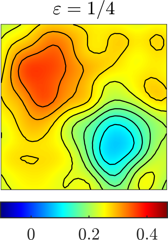
Refer to caption Refer to caption Refer to caption Refer to caption
Figure 6: EnKF with online iterative modeling error estimation after 500500 iterations for the multiscale parameter ε={1/4,1/8,1/16,1/32}\varepsilon=\{1/4,1/8,1/16,1/32\}.

6 Conclusion

In this paper we analyzed the ensemble Kalman inversion methodology in the context of inverse problems for multiscale elliptic PDEs with tensors highly oscillatory at a scale ε≪1\varepsilon\ll 1. The multiscale algorithm we propose relies on the EnKF, on a surrogate homogenized forward operator and on numerical homogenization techniques such as the FE-HMM. It guarantees a significant reduction in computational cost for problems which would be otherwise computationally involved or unfeasible. In Theorem 1 we have shown that the ensemble of particles approximating the unknown parameter generated by our multiscale algorithm converges to the ensemble generated by the true model as the small scale parameter ε\varepsilon and the numerical discretization parameter hh go to zero. Furthermore in a Bayesian framework, we have shown in Theorem 2 that the discrete probability measure based on the ensemble originating from our multiscale algorithm converges to the measure generated by the true model, again as ε\varepsilon and hh go to zero. Hence when ε≪1\varepsilon\ll 1 and the full model is expensive to solve, the multiscale numerical method we propose is both accurate and efficient to recover an unknown parameter in multiscale elliptic PDEs. Moreover, we equipped our method with a technique which allows to account for the discrepancy between the artificial homogenized surrogate forward model and the true multiscale data, thus alleviating the effects of model misspecification. This technique requires additional offline or online computations involving the numerical solution of the full multiscale problem. The optimal number of such additional solves is quantified in Theorem 3 and Theorem 4. In particular, we have proved that the number of solves needed to reach any required accuracy tends to zero when the small scale parameter ε\varepsilon and the numerical discretization parameter hh vanish. Hence, we can conclude that accounting for model misspecification is particularly beneficial for mid-range values of ε\varepsilon, when a small number of full solves should be computationally affordable. The efficiency and usefulness of the multiscale algorithm have been further demonstrated through a series of numerical experiments.

Appendix

Proof of Lemma 1

Let u1,u2∈ℝMu_{1},u_{2}\in\mathbb{R}^{M}, and p1=𝒮⁡(u1)p_{1}=\mathcal{S}(u_{1}), p2=𝒮⁡(u2)p_{2}=\mathcal{S}(u_{2}). From the weak formulations of (21) we get that

∫Ω(Au1∇p1−Au2∇p2)⋅∇v=0for all v∈H01(Ω),\int_{\Omega}\big(A_{u_{1}}\nabla p_{1}-A_{u_{2}}\nabla p_{2}\big)\cdot\nabla v=0\qquad\text{for all }v\in H^{1}_{0}(\Omega),

which yields

∫ΩAu1(∇p1−∇p2)⋅∇v=−∫Ω(Au1−Au2)∇p2⋅∇v.\int_{\Omega}A_{u_{1}}(\nabla p_{1}-\nabla p_{2})\cdot\nabla v=-\int_{\Omega}(A_{u_{1}}-A_{u_{2}})\nabla p_{2}\cdot\nabla v.

Then choosing v=p1−p2v=p_{1}-p_{2}, by the hypotheses on AuA_{u} and applying the Hölder inequality we obtain

α​‖∇p1−∇p2‖L2​(Ω,ℝd)2≤M​‖u1−u2‖2​‖∇p2‖L2​(Ω,ℝd)​‖∇p1−∇p2‖L2​(Ω,ℝd),\alpha\left\|\nabla p_{1}-\nabla p_{2}\right\|_{L^{2}(\Omega;\mathbb{R}^{d})}^{2}\leq M\left\|u_{1}-u_{2}\right\|_{2}\left\|\nabla p_{2}\right\|_{L^{2}(\Omega;\mathbb{R}^{d})}\left\|\nabla p_{1}-\nabla p_{2}\right\|_{L^{2}(\Omega;\mathbb{R}^{d})},

which due a standard coercivity argument implies

‖∇p1−∇p2‖L2​(Ω,ℝd)≤M​Cpα2​‖f‖L2​(Ω)​‖u1−u2‖2,\left\|\nabla p_{1}-\nabla p_{2}\right\|_{L^{2}(\Omega;\mathbb{R}^{d})}\leq\frac{MC_{p}}{\alpha^{2}}\left\|f\right\|_{L^{2}(\Omega)}\left\|u_{1}-u_{2}\right\|_{2}, (79)

where CpC_{p} is the Poincaré constant associated to the domain Ω\Omega. Hence (79) shows that 𝒮\mathcal{S} is Lipschitz with constant

L𝒮=M​Cpα2​‖f‖L2​(Ω).L_{\mathcal{S}}=\frac{MC_{p}}{\alpha^{2}}\left\|f\right\|_{L^{2}(\Omega)}.

Finally, since 𝒢\mathcal{G} is the composition of two Lipschitz operators, we deduce that it is also Lipschitz with constant L𝒢=L𝒪​L𝒮L_{\mathcal{G}}=L_{\mathcal{O}}L_{\mathcal{S}}. ∎

Proof of Lemma 2

Let us consider an ensemble u∈𝒰J,Mu\in\mathcal{U}_{J,M} with particles u(j)∈ℝMu^{(j)}\in\mathbb{R}^{M}, for j=1,…,Jj=1,\ldots,J. For each particle we have

‖𝒢ε​(u(j))−𝒢0​(u(j))‖2=‖𝒪⁡(𝒮ε​(u(j)))−𝒪⁡(𝒮0​(u(j)))‖2≤C𝒪​‖pε​(u(j))−p0​(u(j))‖L2​(Ω),\left\|\mathcal{G}^{\varepsilon}(u^{(j)})-\mathcal{G}^{0}(u^{(j)})\right\|_{2}=\left\|\mathcal{O}(\mathcal{S}^{\varepsilon}(u^{(j)}))-\mathcal{O}(\mathcal{S}^{0}(u^{(j)}))\right\|_{2}\leq C_{\mathcal{O}}\left\|p^{\varepsilon}(u^{(j)})-p^{0}(u^{(j)})\right\|_{L^{2}(\Omega)}, (80)

where we write explicitly the dependence of the solutions pεp^{\varepsilon} and p0p^{0} on the particle they are generated by. Due to homogenization theory, we have that pε​(u(j))⇀p0​(u(j))p^{\varepsilon}(u^{(j)})\rightharpoonup p^{0}(u^{(j)}) in H01​(Ω)H^{1}_{0}(\Omega) for all j=1,…,Jj=1,\dots,J, and therefore pε​(u(j))→p0​(u(j))p^{\varepsilon}(u^{(j)})\to p^{0}(u^{(j)}) in L2​(Ω)L^{2}(\Omega), which implies

e⁡(ε,u)=1J​∑j=1J‖𝒢ε​(u(j))−𝒢0​(u(j))‖2≤C𝒪J​∑j=1J‖pε​(u(j))−p0​(u(j))‖L2​(Ω)→0.e(\varepsilon,u)=\frac{1}{J}\sum_{j=1}^{J}\left\|\mathcal{G}^{\varepsilon}(u^{(j)})-\mathcal{G}^{0}(u^{(j)})\right\|_{2}\leq\frac{C_{\mathcal{O}}}{J}\sum_{j=1}^{J}\left\|p^{\varepsilon}(u^{(j)})-p^{0}(u^{(j)})\right\|_{L^{2}(\Omega)}\to 0.

Moreover, if the solution of the homogenized problem p0p^{0} is sufficiently smooth independently of uu, namely p0∈H2​(Ω)p^{0}\in H^{2}(\Omega), letting C>0C>0 be a constant independent of ε\varepsilon, we have by [12] for all j=1,…,Jj=1,\dots,J

‖pε​(u(j))−p0​(u(j))‖L2​(Ω)≤C​ε,\left\|p^{\varepsilon}(u^{(j)})-p^{0}(u^{(j)})\right\|_{L^{2}(\Omega)}\leq C\varepsilon,

which implies

e⁡(ε,u)=1J​∑j=1J‖𝒢ε​(u(j))−𝒢0​(u(j))‖2≤C𝒪J​∑j=1J‖pε​(u(j))−p0​(u(j))‖L2​(Ω)≤C𝒪​C​ε,e(\varepsilon,u)=\frac{1}{J}\sum_{j=1}^{J}\left\|\mathcal{G}^{\varepsilon}(u^{(j)})-\mathcal{G}^{0}(u^{(j)})\right\|_{2}\leq\frac{C_{\mathcal{O}}}{J}\sum_{j=1}^{J}\left\|p^{\varepsilon}(u^{(j)})-p^{0}(u^{(j)})\right\|_{L^{2}(\Omega)}\leq C_{\mathcal{O}}C\varepsilon,

and defining K=C𝒪​CK=C_{\mathcal{O}}C gives the desired result. ∎

Proof of Lemma 3

First, for all x∈BR​(u∗)x\in B_{R}(u^{*}) we have

‖x‖2\displaystyle\left\|x\right\|_{2} ≤‖x−u∗‖2+‖u∗‖2≤R+‖u∗‖2≕m,\displaystyle\leq\left\|x-u^{*}\right\|_{2}+\left\|u^{*}\right\|_{2}\leq R+\left\|u^{*}\right\|_{2}\eqqcolon m, (81)
‖𝒢⁡(x)‖2\displaystyle\left\|\mathcal{G}(x)\right\|_{2} ≤‖𝒢⁡(x)−𝒢⁡(u∗)‖2+‖𝒢⁡(u∗)‖2≤C𝒢​‖x−u∗‖2+‖𝒢⁡(u∗)‖2≤C𝒢​R+‖𝒢⁡(u∗)‖2≕M.\displaystyle\leq\left\|\mathcal{G}(x)-\mathcal{G}(u^{*})\right\|_{2}+\left\|\mathcal{G}(u^{*})\right\|_{2}\leq C_{\mathcal{G}}\left\|x-u^{*}\right\|_{2}+\left\|\mathcal{G}(u^{*})\right\|_{2}\leq C_{\mathcal{G}}R+\left\|\mathcal{G}(u^{*})\right\|_{2}\eqqcolon M.

We can also deduce the same bounds for the mean values

‖u¯‖2≤1J​∑j=1J‖u(j)‖2≤m,and‖𝒢¯‖2≤1J​∑j=1J‖𝒢⁡(u(j))‖2≤M.\left\|\bar{u}\right\|_{2}\leq\frac{1}{J}\sum_{j=1}^{J}\left\|u^{(j)}\right\|_{2}\leq m,\qquad\text{and}\qquad\left\|\bar{\mathcal{G}}\right\|_{2}\leq\frac{1}{J}\sum_{j=1}^{J}\left\|\mathcal{G}(u^{(j)})\right\|_{2}\leq M. (82)

Then by (81) and (82) we get

‖Cu​p​(u)‖2=\displaystyle\left\|C^{up}(u)\right\|_{2}= supx∈ℝL:‖x‖2=1‖1J∑j=1J(u(j)−u¯)(𝒢(u(j))−𝒢¯)Tx‖2\displaystyle\;\sup_{x\in\mathbb{R}^{L}\colon\left\|x\right\|_{2}=1}\left\lVert\frac{1}{J}\sum_{j=1}^{J}(u^{(j)}-\bar{u})(\mathcal{G}(u^{(j)})-\bar{\mathcal{G}})^{T}x\right\rVert_{2}
≤\displaystyle\leq 1J​∑j=1J(‖𝒢⁡(u(j))‖2+‖𝒢¯‖2)​(‖u(j)‖2+‖u¯‖2)\displaystyle\;\frac{1}{J}\sum_{j=1}^{J}\left(\left\|\mathcal{G}(u^{(j)})\right\|_{2}+\left\|\bar{\mathcal{G}}\right\|_{2}\right)\left(\left\|u^{(j)}\right\|_{2}+\left\|\bar{u}\right\|_{2}\right)
≤\displaystyle\leq  4​M​m,\displaystyle\;4Mm,

and defining C1=4​M​mC_{1}=4Mm we get (i)(i). The argument is similar for the matrix Cp​p​(u)C^{pp}(u), for which we have

‖Cp​p​(u)‖2≤1J​∑j=1J(‖𝒢⁡(u(j))‖2+‖𝒢¯‖2)2≤4​M2,\left\|C^{pp}(u)\right\|_{2}\leq\frac{1}{J}\sum_{j=1}^{J}\left(\left\|\mathcal{G}(u^{(j)})\right\|_{2}+\left\|\bar{\mathcal{G}}\right\|_{2}\right)^{2}\leq 4M^{2},

and defining C2=4​M2C_{2}=4M^{2} we get (i​i)(ii). Before proving (i​i​i)(iii) and (i​v)(iv), we need the following estimates for two ensemble of particles u1u_{1} and u2u_{2}

‖u¯1−u¯2‖2\displaystyle\left\|\bar{u}_{1}-\bar{u}_{2}\right\|_{2} =‖1J​∑j=1J(u1(j)−u2(j))‖2≤1J​∑j=1J‖u1(j)−u2(j)‖2=‖u1−u2‖,\displaystyle=\left\lVert\frac{1}{J}\sum_{j=1}^{J}(u_{1}^{(j)}-u_{2}^{(j)})\right\rVert_{2}\leq\frac{1}{J}\sum_{j=1}^{J}\left\|u_{1}^{(j)}-u_{2}^{(j)}\right\|_{2}=\left\|u_{1}-u_{2}\right\|, (83)
‖𝒢¯1−𝒢¯2‖2\displaystyle\left\|\bar{\mathcal{G}}_{1}-\bar{\mathcal{G}}_{2}\right\|_{2} =‖1J​∑j=1J(𝒢⁡(u1(j))−𝒢⁡(u2(j)))‖2≤C𝒢J​∑j=1J‖u1(j)−u2(j)‖2=C𝒢​‖u1−u2‖.\displaystyle=\left\lVert\frac{1}{J}\sum_{j=1}^{J}(\mathcal{G}(u_{1}^{(j)})-\mathcal{G}(u_{2}^{(j)}))\right\rVert_{2}\leq\frac{C_{\mathcal{G}}}{J}\sum_{j=1}^{J}\left\|u_{1}^{(j)}-u_{2}^{(j)}\right\|_{2}=C_{\mathcal{G}}\left\|u_{1}-u_{2}\right\|.

Then we have

‖Cu​p​(u1)−Cu​p​(u2)‖2\displaystyle\left\|C^{up}(u_{1})-C^{up}(u_{2})\right\|_{2} (84)
=supx∈ℝL:‖x‖2=1‖1J∑j=1J[(u1(j)−u¯1)(𝒢(u1(j))−𝒢¯1)Tx−(u2(j)−u¯2)(𝒢(u2(j))−𝒢¯2)Tx]‖2\displaystyle=\sup_{x\in\mathbb{R}^{L}\colon\left\|x\right\|_{2}=1}\left\lVert\frac{1}{J}\sum_{j=1}^{J}\left[(u_{1}^{(j)}-\bar{u}_{1})(\mathcal{G}(u_{1}^{(j)})-\bar{\mathcal{G}}_{1})^{T}x-(u_{2}^{(j)}-\bar{u}_{2})(\mathcal{G}(u_{2}^{(j)})-\bar{\mathcal{G}}_{2})^{T}x\right]\right\rVert_{2}
≤1J​∑j=1J(‖u1(j)‖2+‖u¯1‖2)​(‖𝒢⁡(u1(j))−𝒢⁡(u2(j))‖2+‖𝒢¯2−𝒢¯1‖2)\displaystyle\leq\frac{1}{J}\sum_{j=1}^{J}\left(\left\|u_{1}^{(j)}\right\|_{2}+\left\|\bar{u}_{1}\right\|_{2}\right)\left(\left\|\mathcal{G}(u_{1}^{(j)})-\mathcal{G}(u_{2}^{(j)})\right\|_{2}+\left\|\bar{\mathcal{G}}_{2}-\bar{\mathcal{G}}_{1}\right\|_{2}\right)
+1J∑j=1J(‖u1(j)−u2(j)‖2+‖u¯2−u¯1‖2)(‖𝒢(u2(j))‖2+‖𝒢¯2‖2),\displaystyle+\frac{1}{J}\sum_{j=1}^{J}\left(\left\|u_{1}^{(j)}-u_{2}^{(j)}\right\|_{2}+\left\|\bar{u}_{2}-\bar{u}_{1}\right\|_{2}\right)\left(\left\|\mathcal{G}(u_{2}^{(j)})\right\|_{2}+\left\|\bar{\mathcal{G}}_{2}\right\|_{2}\right),

and since 𝒢\mathcal{G} is Lipschitz and due to (81), (82), (83), we obtain

‖Cu​p​(u1)−Cu​p​(u2)‖2\displaystyle\left\|C^{up}(u_{1})-C^{up}(u_{2})\right\|_{2} ≤2​m​(C𝒢​J​‖u1−u2‖+C𝒢​‖u1−u2‖)+(J⁡‖u1−u2‖+‖u1−u2‖)​2​M\displaystyle\leq 2m(C_{\mathcal{G}}J\left\|u_{1}-u_{2}\right\|+C_{\mathcal{G}}\left\|u_{1}-u_{2}\right\|)+(J\left\|u_{1}-u_{2}\right\|+\left\|u_{1}-u_{2}\right\|)2M
≤2​(J+1)​(m​C𝒢+M)​‖u1−u2‖,\displaystyle\leq 2(J+1)(mC_{\mathcal{G}}+M)\left\|u_{1}-u_{2}\right\|,

and defining C3=2​(J+1)​(m​C𝒢+M)C_{3}=2(J+1)(mC_{\mathcal{G}}+M) we get (i​i​i)(iii). The argument is similar for the matrix Cp​p​(u)C^{pp}(u), for which we have

‖Cp​p​(u1)−Cp​p​(u2)‖2\displaystyle\left\|C^{pp}(u_{1})-C^{pp}(u_{2})\right\|_{2} ≤1J​∑j=1J(‖𝒢⁡(u1(j))‖+‖𝒢¯1‖2)​(‖𝒢⁡(u1(j))−𝒢⁡(u2(j))‖2+‖𝒢¯2−𝒢¯1‖2)\displaystyle\leq\frac{1}{J}\sum_{j=1}^{J}\left(\left\|\mathcal{G}(u_{1}^{(j)})\right\|+\left\|\bar{\mathcal{G}}_{1}\right\|_{2}\right)\left(\left\|\mathcal{G}(u_{1}^{(j)})-\mathcal{G}(u_{2}^{(j)})\right\|_{2}+\left\|\bar{\mathcal{G}}_{2}-\bar{\mathcal{G}}_{1}\right\|_{2}\right) (85)
+1J∑j=1J(‖𝒢(u1(j))−𝒢(u2(j))‖2+‖𝒢¯2−𝒢¯1‖2)(‖𝒢(u2(j))‖+‖𝒢¯2‖)\displaystyle+\frac{1}{J}\sum_{j=1}^{J}\left(\left\|\mathcal{G}(u_{1}^{(j)})-\mathcal{G}(u_{2}^{(j)})\right\|_{2}+\left\|\bar{\mathcal{G}}_{2}-\bar{\mathcal{G}}_{1}\right\|_{2}\right)\left(\left\|\mathcal{G}(u_{2}^{(j)})\right\|+\left\|\bar{\mathcal{G}}_{2}\right\|\right)
≤4​(J+1)​M​C𝒢,\displaystyle\leq 4(J+1)MC_{\mathcal{G}},

and defining C4=4​(J+1)​M​C𝒢C_{4}=4(J+1)MC_{\mathcal{G}} we get (i​v)(iv), which concludes the proof. ∎

Proof of Lemma 5

Let us consider an ensemble u∈𝒰J,Mu\in\mathcal{U}_{J,M} with particles u(j)∈ℝMu^{(j)}\in\mathbb{R}^{M}, for j=1,…,Jj=1,\ldots,J. For each particle we have

‖𝒢h0​(u(j))−𝒢0​(u(j))‖2=‖𝒪⁡(𝒮h0​(u(j)))−𝒪⁡(𝒮0​(u(j)))‖2≤C𝒪​‖ph0​(u(j))−p0​(u(j))‖L2​(Ω),\left\|\mathcal{G}^{0}_{h}(u^{(j)})-\mathcal{G}^{0}(u^{(j)})\right\|_{2}=\left\|\mathcal{O}(\mathcal{S}^{0}_{h}(u^{(j)}))-\mathcal{O}(\mathcal{S}^{0}(u^{(j)}))\right\|_{2}\leq C_{\mathcal{O}}\left\|p^{0}_{h}(u^{(j)})-p^{0}(u^{(j)})\right\|_{L^{2}(\Omega)}, (86)

where we write explicitly the dependence of the solutions p0p^{0} and ph0p^{0}_{h} on the particle they are generated by. Then due to standard a priori error estimates of FEM (see e.g. [7, Theorem 3.2.5]) and higher order boundary regularity results for elliptic partial differential equations (see e.g. [9, Theorem 6.3.5]) we have for all j=1,…,Jj=1,\ldots,J

‖ph0​(u(j))−p0​(u(j))‖L2​(Ω)≤C​|p0​(u(j))|Hs+1​(Ω)​hs+1≤C​‖f‖Hq−1​(Ω)​hs+1,\left\|p^{0}_{h}(u^{(j)})-p^{0}(u^{(j)})\right\|_{L^{2}(\Omega)}\leq C\left\lvert p^{0}(u^{(j)})\right\rvert_{H^{s+1}(\Omega)}h^{s+1}\leq C\left\|f\right\|_{H^{q-1}(\Omega)}h^{s+1},

where C>0C>0 is a constant independent of hh. Therefore, we obtain

e~​(h,u)=1J​∑j=1J‖𝒢h0​(u(j))−𝒢0​(u(j))‖2≤C𝒪​C​‖f‖Hq−1​(Ω)​hs+1,\tilde{e}(h,u)=\frac{1}{J}\sum_{j=1}^{J}\left\|\mathcal{G}^{0}_{h}(u^{(j)})-\mathcal{G}^{0}(u^{(j)})\right\|_{2}\leq C_{\mathcal{O}}C\left\|f\right\|_{H^{q-1}(\Omega)}h^{s+1}, (87)

and defining K~=C𝒪​C​‖f‖Hq−1​(Ω)\tilde{K}=C_{\mathcal{O}}C\left\|f\right\|_{H^{q-1}(\Omega)} gives the desired result. ∎

Proof of Lemma 7

We follow the same steps of the proof of Theorem 5.9 in [16]. Let us first recall the duality formula for the Wasserstein distance with p=1p=1

W1,s​(μn,μ)=supφ∈Φ{∫BR​(u∗)φ​d​(μn−μ)},W_{1,s}(\mu_{n},\mu)=\sup_{\varphi\in\Phi}\left\{\int_{B_{R}(u^{*})}\varphi d(\mu_{n}-\mu)\right\},

where Φ\Phi is the set of all globally Lipschitz continuous functions φ:BR​(u∗)→ℝ\varphi\colon B_{R}(u^{*})\to\mathbb{R} with Lipschitz constant CLip≤1C_{\mathrm{Lip}}\leq 1. Note that if φ∈Φ\varphi\in\Phi, then also −φ∈Φ-\varphi\in\Phi. Hence we deduce that

W1,s​(μn,μ)=supφ∈Φ{|∫BR​(u∗)φ​d​(μn−μ)|}.W_{1,s}(\mu_{n},\mu)=\sup_{\varphi\in\Phi}\left\{\left|\int_{B_{R}(u^{*})}\varphi d(\mu_{n}-\mu)\right|\right\}. (88)

Then we have

supφ∈Φ𝔼ξ​[|∫BR​(u∗)φ​d​(μn−μ)|]≤𝔼ξ​[supφ∈Φ{|∫BR​(u∗)φ​d​(μn−μ)|}]=𝔼ξ​[W1,s​(μn,μ)],\sup_{\varphi\in\Phi}\mathbb{E}_{\xi}\left[\left|\int_{B_{R}(u^{*})}\varphi d(\mu_{n}-\mu)\right|\right]\leq\mathbb{E}_{\xi}\left[\sup_{\varphi\in\Phi}\left\{\left|\int_{B_{R}(u^{*})}\varphi d(\mu_{n}-\mu)\right|\right\}\right]=\mathbb{E}_{\xi}[W_{1,s}(\mu_{n},\mu)], (89)

where the right hand side vanishes by hypothesis. Therefore we obtain

𝔼ξ​[|∫BR​(u∗)φ​d​μn−∫BR​(u∗)φ​𝑑μ|]→0,\mathbb{E}_{\xi}\left[\left|\int_{B_{R}(u^{*})}\varphi d\mu_{n}-\int_{B_{R}(u^{*})}\varphi d\mu\right|\right]\to 0, (90)

for all φ∈Φ\varphi\in\Phi. Finally, we extend (90) to all Lipschitz functions by linearity and to all bounded continuous functions by density, thus proving the desired result. ∎

References

  • [1] A. Abdulle, A priori and a posteriori error analysis for numerical homogenization: a unified framework, Ser. Contemp. Appl. Math. CAM, 16 (2011), pp. 280–305.
  • [2] A. Abdulle and A. Di Blasio, Numerical homogenization and model order reduction for multiscale inverse problems, Multiscale Model. Simul., 17 (2019), pp. 399–433.
  • [3]  , A Bayesian Numerical Homogenization Method for Elliptic Multiscale Inverse Problems, SIAM/ASA J. Uncertain. Quantif., 8 (2020), pp. 414–450.
  • [4] A. Abdulle, W. E, B. Engquist, and E. Vanden-Eijnden, The heterogeneous multiscale method, Acta Numer., 21 (2012), pp. 1–87.
  • [5] D. Calvetti, M. Dunlop, E. Somersalo, and A. Stuart, Iterative updating of model error for Bayesian inversion, Inverse Problems, 34 (2018), pp. 025008, 38.
  • [6] D. Calvetti, O. Ernst, and E. Somersalo, Dynamic updating of numerical model discrepancy using sequential sampling, Inverse Problems, 30 (2014), pp. 114019, 19.
  • [7] P. G. Ciarlet, The finite element method for elliptic problems., vol. 40 of Classics Appl. Math., SIAM, Philadelphia, 2002.
  • [8] D. Cioranescu and P. Donato, An introduction to homogenization, vol. 17 of Oxford Lecture Series in Mathematics and its Applications, Oxford University Press, New York, 1999.
  • [9] L. C. Evans, Partial differential equations, vol. 19 of Graduate Studies in Mathematics, American Mathematical Society, Providence, RI, second ed., 2010.
  • [10] G. Evensen, Sequential data assimilation with a nonlinear quasi-geostrophic model using Monte Carlo methods to forecast error statistics, J. Geophys. Res., (1994), pp. 10143–10162.
  • [11] M. A. Iglesias, K. J. H. Law, and A. M. Stuart, Ensemble Kalman methods for inverse problems, Inverse Problems, 29 (2013), pp. 045001, 20.
  • [12] S. Moskow and M. Vogelius, First-order corrections to the homogenised eigenvalues of a periodic composite medium. a convergence proof, Proc. Roy. Soc. Edinburgh, 127A (1997), pp. 1263–1299.
  • [13] J. Nolen and G. Papanicolaou, Fine scale uncertainty in parameter estimation for elliptic equations, Inverse Problems, 25 (2009), pp. 115021, 22.
  • [14] J. Nolen, G. A. Pavliotis, and A. M. Stuart, Multiscale modeling and inverse problems, in Numerical analysis of multiscale problems, vol. 83 of Lect. Notes Comput. Sci. Eng., Springer, Heidelberg, 2012, pp. 1–34.
  • [15] S. Salsa, Partial differential equations in action, vol. 99 of Unitext, Springer, [Cham], third ed., 2016. From modelling to theory, La Matematica per il 3+2.
  • [16] F. Santambrogio, Optimal transport for applied mathematicians, vol. 87 of Progress in Nonlinear Differential Equations and their Applications, Birkhäuser/Springer, Cham, 2015. Calculus of variations, PDEs, and modeling.
  • [17] C. Schillings and A. M. Stuart, Analysis of the ensemble Kalman filter for inverse problems, SIAM J. Numer. Anal., 55 (2017), pp. 1264–1290.
  • [18] A. M. Stuart, Inverse problems: a Bayesian perspective, Acta Numer., 19 (2010), pp. 451–559.