跳到论文正文
W Papers独立论文阅读器 arXiv:1908.05423 论文正文 计算阅读时间 · 0%
引用这篇论文根据当前论文元数据生成,正式投稿前建议核对。


License: arXiv.org perpetual non-exclusive license
arXiv:1908.05423v5 [cs.IT] 05 Sep 2020

Random phaseless sampling for causal signals in shift-invariant spaces: a zero distribution perspective

Youfa Li    Wenchang Sun Thanks: Youfa˜Li. College of Mathematics and Information Science, Guangxi University, Naning 530004, China. Email: youfalee@hotmail.com Thanks: Wenchang˜Sun. School of Mathematical Sciences and LPMC, Nankai University, Tianjin 300071, China. Email:sunwch@nankai.edu.cn Thanks: Youfa Li is partially supported by Natural Science Foundation of China (Nos: 61961003, 61561006, 11501132), Natural Science Foundation of Guangxi (No: 2019GXNSFAA185035) and the talent project of Education Department of Guangxi Government for Young-Middle-Aged backbone teachers. Wenchang Sun was partially supported by the National Natural Science Foundation of China (11525104, 11531013 and 11761131002).
Abstract

We proved that the phaseless sampling (PLS) in the linear-phase modulated shift-invariant space (SIS) V(eiα⋅φ),α≠0,V(e^{\textbf{i}\alpha\cdot}\varphi),\alpha\neq 0, is impossible even though the real-valued function φ\varphi enjoys the full spark property (so does eiα⋅φe^{\textbf{i}\alpha\cdot}\varphi). Stated another way, the PLS in the complex-generated SISs is essentially different from that in the real-generated ones. Motivated by this, we first establish the condition on the complex-valued generator ϕ\phi such that the PLS of nonseparable causal (NC) signals in V⁡(ϕ)V(\phi) can be achieved by random sampling. The condition is established from the generalized Haar condition (GHC) perspective. Based on the proposed reconstruction approach, it is proved that if the GHC holds then with probability 11, the random sampling density (SD) =3=3 is sufficient for the PLS of NC signals in the complex-generated SISs. For the real-valued case we also prove that, if the GHC holds then with probability 11, the random SD =2=2 is sufficient for the PLS of real-valued NC signals in the real-generated SISs. For the local reconstruction of highly oscillatory signals such as chirps, a great number of deterministic samples are required. Compared with deterministic sampling, the proposed random approach enjoys not only the greater sampling flexibility but the much smaller number of samples. To verify our results, numerical simulations were conducted to reconstruct highly oscillatory NC signals in the chirp-modulated SISs.

Index Terms: 
Random phaseless sampling, complex (real)-generated shift-invariant space, generalized Haar condition, sampling density, highly oscillatory signals.

I Introduction

Phase retrieval (PR) is a nonlinear problem that seeks to reconstruct a signal ff, up to a unimodular scalar, from the intensities of the linear measurements (c.f.[1, 2, 3, 4, 5, 6, 7])

bk:=|⟨f,ak⟩|,k∈Γ,\displaystyle\begin{array}[]{lll}b_{k}:=|\langle f,\textbf{a}_{k}\rangle|,\ k\in\Gamma,\end{array}

where ak\textbf{a}_{k} is called the measurement vector.

As stated in Y. Shechtman et. al [7] one of the reasons for PR in optics is that, for highly oscillatory signals such as optical waves (electromagnetic fields oscillating at 101510^{15} Hz and higher), measuring their phases is very difficult or even impossible for electronic measurement devices. PR has been widely investigated in engineering and mathematical problems such as coherent diffraction imaging ([7, 8, 9]), quantum tomography ([10]), and frame theory ([11, 12]). A concrete PR problem corresponds to the specific signal class 𝒞\mathcal{C} and measurement vectors (e.g. [13, 14, 15, 16, 17, 18, 19]). For example, Alaifari et. al [15] considered the PR of real-valued bandlimited functions by frame measurement vectors. When ff lies in a function class 𝒞\mathcal{C} and ak\textbf{a}_{k} is the shift of the Dirac distribution, then the corresponding PR is the phaseless sampling (PLS for short), modeled as

to reconstruct​f​by the samples​|f⁡(x)|,x∈Ω,\displaystyle\hbox{to reconstruct}\ f\ \hbox{by the samples}\ |f(x)|,x\in\Omega,

up to a unimodular scalar. In what follows, we introduce the recent developments on PLS in shift-invariant spaces (SISs).

I-A Related work

SIS has many applications in signal processing. Please refer to [19, 20, 21, 22] and the references therein for a few examples. For a generator g:ℝ→ℂg:\mathbb{R}\rightarrow\mathbb{C}, its SIS is defined as

V(g):={∑k∈ℤckg(⋅−k):{ck}k∈ℤ∈ℓ2},\displaystyle\begin{array}[]{lll}V(g):=\{\sum_{k\in\mathbb{Z}}c_{k}g(\cdot-k):\{c_{k}\}_{k\in\mathbb{Z}}\in\ell^{2}\},\end{array}

where {ck}k∈ℤ∈ℓ2\{c_{k}\}_{k\in\mathbb{Z}}\in\ell^{2} means ∑k∈ℤ|ck|2<∞.\sum_{k\in\mathbb{Z}}|c_{k}|^{2}<\infty. Recently, PLS in SISs received much attention (e.g.[23, 24, 25, 26, 27, 28]). Particularly, it was investigated for bandlimited signals in Thakur [25], P. Jaming, K. Kellay and R. Perez Iii [28] and C.K. Lai, F. Littmann, E. Weber [29]. Note that the spaces of bandlimited signals are shift-invariant and the corresponding generators (sinc function or its dilations) are infinitely supported (c.f. [30, 31]). Chen, Cheng, Sun and Wang [26] established the PLS of nonseparable (the definition of nonseparability is postponed to section I-B1) real-valued signals in the SIS from a compactly supported generator. W. Sun [24] established the PLS for nonseparable real-valued signals in SISs generated by B-splines.

Note that the generators and signals in [24, 26] are all real-valued, and the sampling is deterministic. Motivated by the results therein we will investigate the random PLS of causal signals in complex (or real)-generated SISs. Here a signal f∈V⁡(g)f\in V(g) is said to be causal if

f=∑k=0∞ckg(⋅−k),c0≠0.\displaystyle\begin{array}[]{lll}f=\sum_{k=0}^{\infty}c_{k}g(\cdot-k),\ c_{0}\neq 0.\end{array}

The set of causal signals in V⁡(g)V(g) is denoted by Vca​(g)V_{\hbox{ca}}(g). Causal signals are an important class of signals (c.f. [19, 32, 33]). Particularly, the Fourier measurement-based PR of causal signals in SISs was addressed in [19]. In what follows, we introduce the motivation.

I-B Motivation

I-B1 Full spark property fails for complex-valued case

Many practical applications require processing signals in the SISs from complex-valued generators such as chirps (e.g.[21, 34]). We will investigate the PLS in complex-generated SISs. To the best of our knowledge, there are few literatures on this topic. We are greatly motivated by Theorem I.1, which will state that the PLS in the complex-generated SISs is essentially different from that in the real-generated ones.

Some denotations and definitions are necessary for Theorem I.1. A nonzero function ff is traditionally denoted as f≢0f\not\equiv 0, and f⁡(x)≠0f(x)\neq 0 means that the point xx is not the zero of ff. The conjugate of a∈ℂa\in\mathbb{C} is denoted by a¯.\bar{a}. The real and imaginary parts of aa are denoted by ℜ⁡(a)\Re(a) and ℑ⁡(a)\Im(a), respectively. Any a≠0a\neq 0 can be denoted by |a|​ei​θ​(a)|a|e^{\textbf{i}\theta(a)} where i, |a||a| and θ⁡(a)\theta(a) are the imaginary unit, modulus and phase, respectively. For phases θ⁡(a)\theta(a) and θ⁡(b)\theta(b), we say that θ⁡(a)=θ⁡(b)\theta(a)=\theta(b) if θ⁡(a)=θ⁡(b)+2​k​π\theta(a)=\theta(b)+2k\pi for a certain k∈ℤ.k\in\mathbb{Z}. Traditionally, the phase of zero can be assigned arbitrarily.

Throughout this paper the complex and real-valued generators are denoted by ϕ\phi and φ\varphi, respectively. Without loss of generality, assume that

supp​(ϕ)⊆(0,s),supp​(φ)⊆(0,s)\displaystyle\hbox{supp}(\phi)\subseteq(0,s),\ \hbox{supp}(\varphi)\subseteq(0,s) (1.4)

with the integer s≥2s\geq 2. A function 0≢f∈V⁡(ϕ)0\not\equiv f\in V(\phi) (or V⁡(φ)V(\varphi)) is separable if there exist 0≢f10\not\equiv f_{1} and 0≢f2∈V⁡(ϕ)0\not\equiv f_{2}\in V(\phi) (or V⁡(φ)V(\varphi)) such that f=f1+f2f=f_{1}+f_{2} and f1​f2≡0f_{1}f_{2}\equiv 0. Clearly, if ff is separable then |f|=|f1+ei​α​f2||f|=|f_{1}+e^{\textbf{i}\alpha}f_{2}| where α∈(0,2​π)\alpha\in(0,2\pi), and consequently it is not distinguishable from f1+ei​α​f2f_{1}+e^{\textbf{i}\alpha}f_{2} by the samples of |f||f|.

For the above real-valued generator φ\varphi, if the matrix

(φ⁡(xk+n))1≤k≤2​s−1,0≤n≤s−1\displaystyle\begin{array}[]{lllllllllllllllll}\big(\varphi(x_{k}+n)\big)_{1\leq k\leq 2s-1,0\leq n\leq s-1}\end{array}

is full spark (c.f. [35, 36]) for any 2​s−12s-1 distinct points xk∈(0,1),k=1,…,2s−1x_{k}\in(0,1),k=1,\ldots,2s-1, namely, every s×ss\times s submatrix is nonsingular, then it follows from [26] that the real-valued nonseparable signals in V⁡(φ)V(\varphi) can be determined by sufficiently many samples. The B-spline generators in [24] satisfy the property. However, the following theorem implies that the property is not sufficient for achieving PLS when the generator is complex-valued.

Theorem I.1

Let φ\varphi be real-valued such that supp​(φ)⊆(0,s)\hbox{supp}(\varphi)\subseteq(0,s) and the matrix in (I-B1) is full spark for any 2​s−12s-1 distinct points xk∈(0,1)x_{k}\in(0,1), k=1,…,2​s−1k=1,\ldots,2s-1. Define ϕ:=eiα⋅φ\phi:=e^{\textbf{i}\alpha\cdot}\varphi with α≠0\alpha\neq 0. Then the PLS in Vca​(ϕ)V_{\hbox{ca}}(\phi) can not be achieved despite the fact that ϕ\phi also satisfies the full spark property.

Proof:

It is easy to check that ϕ\phi inherits the full spark property of φ\varphi. It follows from the full spark property that {ϕ(⋅+k):k=0,…,s−1}\{\phi(\cdot+k):k=0,\ldots,s-1\} is linearly independent. We first choose β∈ℝ\beta\in\mathbb{R} such that α−β≠k​π\alpha-\beta\neq k\pi for any k∈ℤ.k\in\mathbb{Z}. Let N≥2N\geq 2. Define a sequence {ck}k=0N\{c_{k}\}^{N}_{k=0} such that c0=1c_{0}=1 and c1=ei​βc_{1}=e^{\textbf{i}\beta}. It is easy to check that {ck}k=0N≠ei​θ^​{ei​2​α​k​c¯k}k=0N\{c_{k}\}^{N}_{k=0}\neq e^{\textbf{i}\widehat{\theta}}\{e^{\textbf{i}2\alpha k}\overline{c}_{k}\}^{N}_{k=0} for any θ^∈[0,2​π)\widehat{\theta}\in[0,2\pi). By the above linear independence, we have ∑k=0Nckϕ(⋅−k)≠ei​θ^∑k=0Nei​2​α​kc¯kϕ(⋅−k)\sum^{N}_{k=0}c_{k}\phi(\cdot-k)\neq e^{\textbf{i}\widehat{\theta}}\sum^{N}_{k=0}e^{\textbf{i}2\alpha k}\overline{c}_{k}\phi(\cdot-k). However, it is easy to check that

|∑k=0Nei​2​α​kc¯kϕ(⋅−k)|=|∑k=0Nckϕ(⋅−k)|.\displaystyle|\sum^{N}_{k=0}e^{\textbf{i}2\alpha k}\overline{c}_{k}\phi(\cdot-k)|=|\sum^{N}_{k=0}c_{k}\phi(\cdot-k)|. (1.6)

In other words, the PLS in Vca​(ϕ)V_{\hbox{ca}}(\phi) can not be achieved. ∎

Motivated by Theorem I.1, we need to establish a condition on the complex-valued generator ϕ\phi such that the PLS in Vca​(ϕ)V_{\hbox{ca}}(\phi) can be achieved. The condition will be established from the zero distribution (or the Lebesgue measure of zero set) perspective. Our motivation for this perspective is introduced in what follows.

I-B2 New perspective: zero distribution-based PLS

We first interpret the full spark property from the zero distribution perspective. For a function system Λ={g0,…,gL−1}\Lambda=\{g_{0},\ldots,g_{L-1}\}, its span space is defined as

span​{Λ}:={∑j=0L−1cj​gj:cj∈ℝ}.\displaystyle\begin{array}[]{lllllllllllllllll}\hbox{span}\{\Lambda\}:=\big\{\sum^{L-1}_{j=0}c_{j}g_{j}:c_{j}\in\mathbb{R}\big\}.\end{array}

It is easy to check that the full spark property of the matrix in (I-B1) is equivalent to that the function system

Λφ:={φ,…,φ(⋅+s−1)}\displaystyle\begin{array}[]{lllllllllllllllll}\Lambda_{\varphi}:=\{\varphi,\ldots,\varphi(\cdot+s-1)\}\end{array}

satisfies the (s−1)(s-1)-Haar condition (HC for short) on (0,1)(0,1) (c.f.[37, 38, 39] for HC). Specifically, Λφ\Lambda_{\varphi} is linearly independent and

sup0≢h∈span​{Λφ}#⁡(𝒵h∩(0,1))≤s−1,\displaystyle\sup_{0\not\equiv h\in\hbox{span}\{\Lambda_{\varphi}\}}\#(\mathcal{Z}_{h}\cap(0,1))\leq s-1, (1.9)

where 𝒵h\mathcal{Z}_{h} is the zero set of hh and #⁡(𝒵h∩(0,1))\#(\mathcal{Z}_{h}\cap(0,1)) is the cardinality of 𝒵h∩(0,1)\mathcal{Z}_{h}\cap(0,1).

Motivated by the above HC, from the zero distribution perspective we will establish the condition on ϕ:=ϕℜ+i​ϕℑ\phi:=\phi_{\Re}+\textbf{i}\phi_{\Im} such that the PLS in Vca​(ϕ)V_{\hbox{ca}}(\phi) can be achieved. Inspired by Theorem I.1, the zero distribution should not be correlated with the functions in span{ϕ,…,ϕ(⋅+s−1)}\hbox{span}\{\phi,\ldots,\phi(\cdot+s-1)\}. Instead we will require in section II that the distribution is related with the functions in span​(Ξϕ)\hbox{span}(\Xi_{\phi}), where

Ξϕ:={ϕℜϕℜ(⋅+k)+ϕℑϕℑ(⋅+k),ϕℜϕℑ(⋅+k)−ϕℑϕℜ(⋅+k)}s−1k=1∪{ϕ2ℜ+ϕ2ℑ}.\displaystyle\begin{array}[]{lllllllllllllllll}\Xi_{\phi}:=\big\{\phi_{\Re}\phi_{\Re}(\cdot+k)+\phi_{\Im}\phi_{\Im}(\cdot+k),\phi_{\Re}\phi_{\Im}(\cdot+k)-\\ \ \ \ \quad\quad\phi_{\Im}\phi_{\Re}(\cdot+k)\big\}^{s-1}_{k=1}\cup\big\{\phi^{2}_{\Re}+\phi^{2}_{\Im}\big\}.\end{array}

More specifically, Ξϕ\Xi_{\phi} is linearly independent and

sup0≢h∈span​{Ξϕ}μ⁡(𝒵h∩(0,1))=0,\displaystyle\sup_{0\not\equiv h\in\hbox{span}\{\Xi_{\phi}\}}\mu(\mathcal{Z}_{h}\cap(0,1))=0, (1.12)

where μ\mu is the Lebesgue measure and span​{Ξϕ}\hbox{span}\{\Xi_{\phi}\} is defined via (I-B2). Clearly, (1.12) (a measure perspective) is essentially different from (1.9) (a cardinality perspective). Compared with the cardinality perspective, we will profit more from the measure perspective. Details on this will be given in section I-E. For simplicity we give the following definitions.

Definition I.2

If (1.12) holds, then we say that the system Ξϕ\Xi_{\phi} satisfies the generalized Haar condition (GHC for short), and ϕ\phi is a complex-valued GHC-generator.

As a counterpart of Definition I.2, we next define the GHC related to the real-valued generator φ\varphi in (1.4).

Definition I.3

If Λφ={φ(⋅+k):k=0,…,s−1}\Lambda_{\varphi}=\{\varphi(\cdot+k):k=0,\ldots,s-1\} in (I-B2) is linearly independent and satisfies

sup0≢h∈span​{Λφ}μ⁡(𝒵h∩(0,1))=0,\displaystyle\sup_{0\not\equiv h\in\hbox{span}\{\Lambda_{\varphi}\}}\mu(\mathcal{Z}_{h}\cap(0,1))=0, (1.13)

then we say that the system Λφ\Lambda_{\varphi} satisfies the GHC, and φ\varphi is a real-valued GHC-generator.

I-C Typical GHC-generators

I-C1 Typical complex-valued GHC-generators

We start with the amplitude-phase form of a complex-valued function. Any function (including a generator for an SIS) F:ℝ⟶ℂF:\mathbb{R}\longrightarrow\mathbb{C} can be written as the general form |F⁡(t)|​ei​θ​(F⁡(t))|F(t)|e^{\textbf{i}\theta(F(t))}, where |F⁡(t)||F(t)| and θ⁡(F⁡(t))\theta(F(t)) (taking values on [0,2​π)[0,2\pi)) are referred to as the amplitude function and the phase (or rotation) function. Therefore, any complex-valued generator for an SIS can be interpreted as the (possibly nonlinear) rotation of a real-valued function.

As mentioned before, one of the reasons for PR in optics is the high oscillation of a signal. Chirps which take the very general form F⁡(t)​ei​λ​ρ​(t)F(t)e^{\textbf{i}\lambda\rho(t)} are the typical class of highly oscillatory signals, where F⁡(t)≥0F(t)\geq 0 and λ\lambda is a (large) base frequency such that the phase function λ​ρ​(t)\lambda\rho(t) is varying rapidly over time (c.f.[40]). As stated in [40], chirps are ubiquitous in nature. They are of interest in applications such as in analysis of echolocation in bats ([41]) and whales ([42, 40]), and in detecting gravitational waves ([40]). They are also applied in ultrafast optics ([43]) and ultrashort laser pulses ([44]).

Many chirps such as those in [34, section 6.3] have the local analytic structure. Employing this, GHC (1.12) can be easily checked. For example, motivated by [34, section 6.3] we take the chirp-generator

ϕ⁡(x)=23​2​π​|b|​e−i​a​(x−2)22​b​e−i​p⁡(x−2)b​cos2⁡π⁡(x−2)4​χ(0,4)​(x),\displaystyle\begin{array}[]{lll}\phi(x)=\frac{2}{3}\sqrt{2\pi|b|}e^{-\textbf{i}\frac{a(x-2)^{2}}{2b}}e^{-\textbf{i}\frac{p(x-2)}{b}}\cos^{2}\frac{\pi(x-2)}{4}\chi_{(0,4)}(x),\end{array}

such that supp​(ϕ)=(0,4)\hbox{supp}(\phi)=(0,4), where a≠0a\neq 0 and χE\chi_{E} is the characteristic function of the set E⊆ℝE\subseteq\mathbb{R}. Clearly, the 77 components of the system Ξϕ\Xi_{\phi} in (I-B2) are essentially the restrictions of analytic functions. Recall that the zero set of any nonzero analytic function has Lebesgue measure zero (c.f. [45]). Hence, if the components gi∈Ξϕg_{i}\in\Xi_{\phi}, i=1,…,7i=1,\ldots,7, are linearly independent on (0,1)(0,1) then ϕ\phi is a complex-valued GHC-generator. The independence can be achieved if there exists (x1,…,x7)∈(0,1)7(x_{1},\ldots,x_{7})\in(0,1)^{7} such that the determinant

|g1​(x1)g2​(x1)…g7​(x1)⋮⋮⋱⋮g1​(x7)g2​(x7)…g7​(x7)|≠0.\displaystyle\left|\begin{array}[]{ccccc}g_{1}(x_{1})&g_{2}(x_{1})&\ldots&g_{7}(x_{1})\\ \vdots&\vdots&\ddots&\vdots\\ g_{1}(x_{7})&g_{2}(x_{7})&\ldots&g_{7}(x_{7})\end{array}\right|\neq 0.

Take the parameters (a,b,p)=(4,0.8,1)(a,b,p)=(4,0.8,1) or (50,0.8,1)(50,0.8,1) for example. Uniformly choosing (x1,…,x7)(x_{1},\ldots,x_{7}) from (0,1)7(0,1)^{7} we found that (I-C1) holds with probability 1.1. Then ϕ\phi in (I-C1) is a complex-valued GHC-generator.

I-C2 Real-valued GHC-generators

If a real-valued generator has the local analytic structure, then we can also address how to check whether it is a GHC-generator by the similar argument as above. The cardinal B-splines and the refinable functions ([46, 47, 48]) having positive masks are the typical examples of real-valued GHC-generators.

I-D Contributions

An infinite discrete set EE is said to have sampling density (SD) if SD=limb−a→∞#⁡([a,b]∩E)b−a<∞\hbox{SD}=\lim_{b-a\rightarrow\infty}\frac{\#([a,b]\cap E)}{b-a}<\infty. Throughout this paper, we require that the random sampling points on any unit interval [n,n+1][n,n+1] obey the uniform distribution. Our contributions include:

(i) From a new perspective—zero distribution, we establish the condition for the PLS of causal signals in the complex-generated SISs. Specifically, Theorem II.5 will state that if ϕ\phi is a complex-valued GHC-generator, then with probability 11 the random SD =3=3 is sufficient for the PLS of nonseparable signals in Vca​(ϕ)V_{\hbox{ca}}(\phi).

(ii) The PLS of nonseparable and real-valued signals in real-generated SISs is also investigated from the zero distribution perspective. Specifically, Theorem III.1 will state that if φ\varphi is a real-valued GHC-generator, then with probability 11 the random SD =2=2 is sufficient for the PLS of nonseparable and real-valued signals in Vca​(φ)V_{\hbox{ca}}(\varphi).

(iii) An alternating approach, termed as phase decoding-coefficient recovery (PD-CR), is established to reconstruct the nonseparable signals in Vca​(ϕ)V_{\hbox{ca}}(\phi) and Vca​(φ)V_{\hbox{ca}}(\varphi). By the random sampling-based PD-CR, Propositions II.6 and III.2 will guarantee that the highly oscillatory signals can be locally reconstructed by using a very small number of samples. More details about this is given in section I-E-2).

I-E Highlights

I-E1 The zero distribution perspective enables us to do PLS in complex-generated Vca​(ϕ)V_{\hbox{ca}}(\phi)

As mentioned in section I-B2, the traditional requirement—full spark property for PLS of real-valued signals can be interpreted by (1.9), a cardinality perspective. Theorem I.1 implies that the property does not work for complex-valued case. Based on GHC (a measure perspective), we establish the PLS of nonseparable signals in Vca​(ϕ)V_{\hbox{ca}}(\phi).

I-E2 Local reconstruction of highly oscillatory signals costs a small number of samples

If φ\varphi or ϕ\phi is highly oscillatory, then the quantities sup0≢h∈span​{Λφ}#⁡(𝒵h∩(0,1))\sup_{0\not\equiv h\in\hbox{span}\{\Lambda_{\varphi}\}}\#(\mathcal{Z}_{h}\cap(0,1)) and sup0≢h∈span​{Ξϕ}#⁡(𝒵h∩(0,1))\sup_{0\not\equiv h\in\hbox{span}\{\Xi_{\phi}\}}\#(\mathcal{Z}_{h}\cap(0,1)) are great. And a great number of deterministic samples are necessary for local reconstruction. However, Propositions II.6 and III.2 will guarantee that the highly oscillatory signals can be locally reconstructed, with probability 11, by using a very small number of random samples. Unlike [24], the number of samples is independent of the above quantities. To make this point, we will give a test signal in section III-C (III-C) and its local restriction in (3.97). Although the restriction is determined by just two coefficients, one needs at least 259 deterministic samples to reconstruct it. By the PD-CR, however, with probability 11 it can be reconstructed by just three random samples.

I-F Organization

Section II concerns on the random PLS of nonseparable signals in Vca​(ϕ)V_{\hbox{ca}}(\phi), where ϕ\phi is a complex-valued GHC-generator. Based on the proposed PD-CR, we proved that when the sampling points obey the uniform distribution and the random SD =3=3, then with probability 11 any nonseparable signal in Vca​(ϕ)V_{\hbox{ca}}(\phi) can be determined up to a unimodular scalar. In section III the PD-CR is modified such that it is more adaptive to the real-valued case. By the modified PD-CR, the real-valued and nonseparable signals in Vca​(φ)V_{\hbox{ca}}(\varphi) can be determined with probability 11 if the random SD =2.=2. To confirm our results numerical simulations are conducted in section II-H and section III-C. For the local reconstruction, Propositions II.6 and III.2 imply that the highly oscillatory signals can be determined, with probability 11, by using a very small number of random samples. We conclude in section IV.

II Random PLS of causal signals in complex-generated SISs

We start with some necessary denotations. As in section I the conjugate of a∈ℂa\in\mathbb{C} is denoted by a¯.\bar{a}. The random variable tt, obeying the uniform distribution on (0,1)(0,1), is denoted by t∼U​(0,1)t\sim\textbf{U}(0,1). Its observed value is denoted by t^.\widehat{t}. For an event 𝔈\mathfrak{E}, its probability and complementary event are denoted by P⁡(𝔈)P(\mathfrak{E}) and 𝔈c\mathfrak{E}^{c}, respectively. For two events 𝔈1\mathfrak{E}_{1} and 𝔈2\mathfrak{E}_{2}, P⁡(𝔈1∩𝔈2)=P⁡(𝔈1|𝔈2)​P​(𝔈2),P(\mathfrak{E}_{1}\cap\mathfrak{E}_{2})=P(\mathfrak{E}_{1}|\mathfrak{E}_{2})P(\mathfrak{E}_{2}), where 𝔈1∩𝔈2\mathfrak{E}_{1}\cap\mathfrak{E}_{2} and P⁡(𝔈1|𝔈2)P(\mathfrak{E}_{1}|\mathfrak{E}_{2}) are the intersection event and conditional probability, respectively.

II-A Preliminary on complex-valued GHC-generator

The following proposition will be helpful for proving Theorem II.5, one of our main theorems.

Proposition II.1

Let ϕ=ϕℜ+i​ϕℑ\phi=\phi_{\Re}+\textbf{i}\phi_{\Im} be a GHC-generator supported on (0,s)(0,s). Then Λϕ,1:={ϕ(⋅+k):k=0,…,s−1}\Lambda_{\phi,1}:=\{\phi(\cdot+k):k=0,\ldots,s-1\} and Λϕ,2:={ϕϕ¯(⋅+k):k=0,…,s−1}\Lambda_{\phi,2}:=\{\phi\bar{\phi}(\cdot+k):k=0,\ldots,s-1\} also satisfy the GHC, namely, (1.12) holds with Ξϕ\Xi_{\phi} being replaced by Λϕ,1\Lambda_{\phi,1} or Λϕ,2\Lambda_{\phi,2}.

Proof:

The proof can be easily concluded by the GHC in (1.12) associated with Ξϕ\Xi_{\phi}. ∎

Note II.2

Theorem I.1 implies that Λϕ,1\Lambda_{\phi,1} satisfying GHC is not sufficient for achieving the PLS in Vca​(ϕ)V_{\hbox{ca}}(\phi). By the same argument as in the proof of Theorem I.1, it is easy to prove that Λϕ,2\Lambda_{\phi,2} is also not sufficient.

II-B Phase decoding-coefficient recovery for Vca​(ϕ)V_{\hbox{ca}}(\phi)

As in section I, Vca​(ϕ)V_{\hbox{ca}}(\phi) is defined by

Vca(ϕ)={∑k=0∞ckϕ(⋅−k):{ck}∈ℓ2,c0≠0,ck∈ℂ}.\displaystyle\begin{array}[]{lll}V_{\hbox{ca}}(\phi)=\{\sum_{k=0}^{\infty}c_{k}\phi(\cdot-k):\{c_{k}\}\in\ell^{2},\ c_{0}\neq 0,c_{k}\in\mathbb{C}\}.\end{array}

For f∈Vca​(ϕ)f\in V_{\hbox{ca}}(\phi), call 𝒩f:=sup{k:ck≠0}\mathcal{N}_{f}:=\sup\{k:c_{k}\neq 0\} the maximum coefficient index of ff. Clearly, if ff is compactly supported (infinitely supported) then 𝒩f<∞(=∞)\mathcal{N}_{f}<\infty(=\infty). On the other hand, if the phases of sufficiently many samples of |f||f| have been decoded, then the reconstruction of ff can be linear. Motivated by this, we will establish an alternating approach: phase decoding-coefficient recovery (PD-CR). Some denotations are necessary for introducing the approach.

As in section I, ϕ\phi is supported on (0,s)(0,s) with the integer s≥2s\geq 2. For n≥1n\geq 1, define the set InI_{n} by

In:={{0,1,…,n−1},1≤n≤s−1,{n−s+1,…,n−1},n≥s.\displaystyle I_{n}:=\left\{\begin{array}[]{lll}\{0,1,\ldots,n-1\},&1\leq n\leq s-1,\\ \{n-s+1,\ldots,n-1\},&n\geq s.\end{array}\right.

For f=∑k=0∞ckϕ(⋅−k)∈Vca(ϕ)f=\sum_{k=0}^{\infty}c_{k}\phi(\cdot-k)\in V_{\hbox{ca}}(\phi), define the auxiliary function vn,fv_{n,f} on (0,1)(0,1) by

vn,f(⋅):=∑k∈Inckϕ(n+⋅−k),\displaystyle\begin{array}[]{lll}v_{n,f}(\cdot):=\sum_{k\in I_{n}}c_{k}\phi(n+\cdot-k),\end{array}

which together with supp​(ϕ)⊆(0,s)\hbox{supp}(\phi)\subseteq(0,s) leads to

f⁡(n+x)=vn,f​(x)+cn​ϕ​(x),x∈(0,1).\displaystyle f(n+x)=v_{n,f}(x)+c_{n}\phi(x),x\in(0,1). (2.22)

Based on vn,fv_{n,f}, define two auxiliary bivariate functions

An,f​(x,y)+Bn,f​(x,y)​i:=|f|​(n+x)|ϕ|2​(x)​[ϕ¯​(x)​ϕ​(y)​v¯n​(y)−v¯n​(x)​|ϕ|2​(y)],\displaystyle\begin{array}[]{lll}A_{n,f}(x,y)+B_{n,f}(x,y)\textbf{i}\\ :=\frac{|f|(n+x)}{|\phi|^{2}(x)}\big[\bar{\phi}(x)\phi(y)\bar{v}_{n}(y)-\bar{v}_{n}(x)|\phi|^{2}(y)\big],\end{array}

and

Cn,f​(x,y):=|f|2​(n+y)−|vn,f|2​(y)+2​ℜ⁡(vn,f​(x)​v¯n,f​(y)​ϕ​(y)ϕ⁡(x))−|ϕ|2​(y)|ϕ|2​(x)​[|f|2​(n+x)+|vn,f|2​(x)],\displaystyle\begin{array}[]{lll}C_{n,f}(x,y)\\ :=|f|^{2}(n+y)-|v_{n,f}|^{2}(y)+2\Re(\frac{v_{n,f}(x)\bar{v}_{n,f}(y)\phi(y)}{\phi(x)})\\ -\frac{|\phi|^{2}(y)}{|\phi|^{2}(x)}[|f|^{2}(n+x)+|v_{n,f}|^{2}(x)],\end{array}

whenever x,y∈(0,1)x,y\in(0,1) such that ϕ⁡(x)≠0\phi(x)\neq 0. The values of the above bivariate functions at (x,y)∈(0,1)2(x,y)\in(0,1)^{2} are correlated via the following equation w.r.t the unknown z∈ℂz\in\mathbb{C}:

(An,f​(x,y)+Bn,f​(x,y)​i)​z2−Cn,f​(x,y)​z+An,f​(x,y)−Bn,f​(x,y)​i=0.\displaystyle\begin{array}[]{lll}(A_{n,f}(x,y)+B_{n,f}(x,y)\textbf{i})z^{2}-C_{n,f}(x,y)z\\ +A_{n,f}(x,y)-B_{n,f}(x,y)\textbf{i}=0.\end{array}

The following lemma states that the solutions to (II-B) can provide a precise feedback on the global phase of {ck}k∈In\{c_{k}\}_{k\in I_{n}}.

Lemma II.3

Let vn,f​(⋅)v_{n,f}(\cdot) and An,f​(⋅,⋅)+Bn,f​(⋅,⋅)​iA_{n,f}(\cdot,\cdot)+B_{n,f}(\cdot,\cdot)\textbf{i} be defined in (II-B) and (II-B), respectively. Define v~n,f​(⋅)\widetilde{v}_{n,f}(\cdot) via (II-B) with {ck}k∈In\{c_{k}\}_{k\in I_{n}} being replaced by {c~k}k∈In:=ei​θ^​{ck}k∈In\{\widetilde{c}_{k}\}_{k\in I_{n}}:=e^{\textbf{i}\widehat{\theta}}\{c_{k}\}_{k\in I_{n}}. Moreover, define A~n,f​(⋅,⋅)+B~n,f​(⋅,⋅)​i\widetilde{A}_{n,f}(\cdot,\cdot)+\widetilde{B}_{n,f}(\cdot,\cdot)\textbf{i} and C~n,f​(⋅,⋅)\widetilde{C}_{n,f}(\cdot,\cdot) via (II-B) and (II-B) with vn,f​(⋅)v_{n,f}(\cdot) being replaced by v~n,f​(⋅)\widetilde{v}_{n,f}(\cdot). For fixed x,y∈(0,1)x,y\in(0,1) and n≥1n\geq 1 such that ϕ⁡(x)≠0\phi(x)\neq 0 and An,f​(x,y)+Bn,f​(x,y)​i≠0A_{n,f}(x,y)+B_{n,f}(x,y)\textbf{i}\neq 0, suppose that the two solutions to (II-B) are z1z_{1} and z2z_{2}. Then the two solutions to

(A~n,f​(x,y)+B~n,f​(x,y)​i)​z2−C~n,f​(x,y)​z+A~n,f​(x,y)−B~n,f​(x,y)​i=0\displaystyle\begin{array}[]{lll}(\widetilde{A}_{n,f}(x,y)+\widetilde{B}_{n,f}(x,y)\textbf{i})z^{2}-\widetilde{C}_{n,f}(x,y)z\\ +\widetilde{A}_{n,f}(x,y)-\widetilde{B}_{n,f}(x,y)\textbf{i}=0\end{array}

are ei​θ^​z1e^{\textbf{i}\widehat{\theta}}z_{1} and ei​θ^​z2e^{\textbf{i}\widehat{\theta}}z_{2}.

Proof:

Through the direct calculation we have vn,f​(x)​v¯n,f​(y)​ϕ​(y)ϕ⁡(x)=v~n,f​(x)​v~¯n,f​(y)​ϕ​(y)ϕ⁡(x)\frac{v_{n,f}(x)\bar{v}_{n,f}(y)\phi(y)}{\phi(x)}=\frac{\widetilde{v}_{n,f}(x)\bar{\widetilde{v}}_{n,f}(y)\phi(y)}{\phi(x)} and

Cn,f(x,y)=C~n,f(x,y),A~n,f​(x,y)+B~n,f​(x,y)​iAn,f​(x,y)+Bn,f​(x,y)​i=e−i​θ^.\displaystyle\begin{array}[]{lll}C_{n,f}(x,y)=\widetilde{C}_{n,f}(x,y),\frac{\widetilde{A}_{n,f}(x,y)+\widetilde{B}_{n,f}(x,y)\textbf{i}}{A_{n,f}(x,y)+B_{n,f}(x,y)\textbf{i}}=e^{-\textbf{i}\widehat{\theta}}.\end{array}

On the other hand,

z1,z2=Cn,f​(x,y)±Cn,f2​(x,y)−4​|An,f​(x,y)+Bn,f​(x,y)​i|22​(An,f​(x,y)+Bn,f​(x,y)​i),\displaystyle\begin{array}[]{lll}z_{1},z_{2}\\ =\frac{C_{n,f}(x,y)\pm\sqrt{C^{2}_{n,f}(x,y)-4|A_{n,f}(x,y)+B_{n,f}(x,y)\textbf{i}|^{2}}}{2(A_{n,f}(x,y)+B_{n,f}(x,y)\textbf{i})},\end{array}

which together with (II-B) leads to that the two solutions to (II.3) are ei​θ^​z1e^{\textbf{i}\widehat{\theta}}z_{1} and ei​θ^​z2e^{\textbf{i}\widehat{\theta}}z_{2}. ∎

Based on Lemma II.3, the following theorem concerns on a guarantee for decoding phases.

Theorem II.4

Let f∈Vca​(ϕ)f\in V_{\hbox{ca}}(\phi). Assume that all the samples

{|f(t^0)|}∪{|f(n+t^nj)|:j=1,2,3,n=1,…,𝒩f+s−1}\displaystyle\begin{array}[]{lll}\{|f(\widehat{t}_{0})|\}\cup\big\{|f(n+\widehat{t}_{n_{j}})|:j=1,2,3,n=1,\ldots,\\ \quad\quad\quad\quad\quad\quad\quad\quad\quad\quad\quad\ \mathcal{N}_{f}+s-1\big\}\end{array}

are nonzeros where t^0,t^nj∈(0,1).\widehat{t}_{0},\widehat{t}_{n_{j}}\in(0,1). Then the corresponding phases {θ⁡(f⁡(t^0))}∪{θ⁡(f⁡(n+t^nj))}n,j\{\theta(f(\widehat{t}_{0}))\}\cup\{\theta(f(n+\widehat{t}_{n_{j}}))\}_{n,j} can be determined (up to a global real-valued number) if for every n∈{1,2,…,𝒩f+s−1}n\in\{1,2,\ldots,\mathcal{N}_{f}+s-1\}, ϕ⁡(t^n1)≠0\phi(\widehat{t}_{n_{1}})\neq 0 and the equation system

{(An,f​(t^n1,t^n2)+Bn,f​(t^n1,t^n2)​i)​z2−Cn,f​(t^n1,t^n2)​z+An,f​(t^n1,t^n2)−Bn,f​(t^n1,t^n2)​i=0,(An,f​(t^n1,t^n3)+Bn,f​(t^n1,t^n3)​i)​z2−Cn,f​(t^n1,t^n3)​z+An,f​(t^n1,t^n3)−Bn,f​(t^n1,t^n3)​i=0,\displaystyle\left\{\begin{array}[]{lll}(A_{n,f}(\widehat{t}_{n_{1}},\widehat{t}_{n_{2}})+B_{n,f}(\widehat{t}_{n_{1}},\widehat{t}_{n_{2}})\textbf{i})z^{2}-C_{n,f}(\widehat{t}_{n_{1}},\widehat{t}_{n_{2}})z\\ +A_{n,f}(\widehat{t}_{n_{1}},\widehat{t}_{n_{2}})-B_{n,f}(\widehat{t}_{n_{1}},\widehat{t}_{n_{2}})\textbf{i}=0,\\ (A_{n,f}(\widehat{t}_{n_{1}},\widehat{t}_{n_{3}})+B_{n,f}(\widehat{t}_{n_{1}},\widehat{t}_{n_{3}})\textbf{i})z^{2}-C_{n,f}(\widehat{t}_{n_{1}},\widehat{t}_{n_{3}})z\\ +A_{n,f}(\widehat{t}_{n_{1}},\widehat{t}_{n_{3}})-B_{n,f}(\widehat{t}_{n_{1}},\widehat{t}_{n_{3}})\textbf{i}=0,\end{array}\right.

w.r.t the the unknown z∈ℂz\in\mathbb{C} has a unique solution.

Proof:

As previously, denote f=∑k=0∞ckϕ(⋅−k)f=\sum_{k=0}^{\infty}c_{k}\phi(\cdot-k). We prove the theorem recursively on nn. Suppose that

θ⁡(f⁡(t^0))=θ0\displaystyle\theta(f(\widehat{t}_{0}))=\theta_{0} (2.40)

is known as the priori information. Then it follows from 0≠f⁡(t^0)=c0​ϕ​(t^0)0\neq f(\widehat{t}_{0})=c_{0}\phi(\widehat{t}_{0}) that

c0=ei​θ0​|f⁡(t^0)|/ϕ⁡(t^0).\displaystyle c_{0}=e^{\textbf{i}\theta_{0}}|f(\widehat{t}_{0})|/\phi(\widehat{t}_{0}). (2.41)

For n=1n=1, we next address how to determine z:=ei​θ​(f⁡(t^11+1))z:=e^{\textbf{i}\theta(f(\widehat{t}_{1_{1}}+1))}. It follows from (2.22) that

{|v1,f​(t^11)+c1​ϕ​(t^11)|=|f⁡(1+t^11)|,|v1,f​(t^12)+c1​ϕ​(t^12)|=|f⁡(1+t^12)|,|v1,f​(t^13)+c1​ϕ​(t^13)|=|f⁡(1+t^13)|,\displaystyle\left\{\begin{array}[]{lll}|v_{1,f}(\widehat{t}_{1_{1}})+c_{1}\phi(\widehat{t}_{1_{1}})|=|f(1+\widehat{t}_{1_{1}})|,\\ |v_{1,f}(\widehat{t}_{1_{2}})+c_{1}\phi(\widehat{t}_{1_{2}})|=|f(1+\widehat{t}_{1_{2}})|,\\ |v_{1,f}(\widehat{t}_{1_{3}})+c_{1}\phi(\widehat{t}_{1_{3}})|=|f(1+\widehat{t}_{1_{3}})|,\end{array}\right.

where v1,f​(t^1j),j=1,2,3,v_{1,f}(\widehat{t}_{1_{j}}),j=1,2,3, are computed by using (II-B) and (2.41) as follows,

v1,f​(t^1j)=ϕ⁡(1+t^1j)​c0=ϕ⁡(1+t^1j)​ei​θ0​|f⁡(t^0)|ϕ⁡(t^0).\displaystyle\begin{array}[]{lll}v_{1,f}(\widehat{t}_{1_{j}})=\phi(1+\widehat{t}_{1_{j}})c_{0}=\frac{\phi(1+\widehat{t}_{1_{j}})e^{\textbf{i}\theta_{0}}|f(\widehat{t}_{0})|}{\phi(\widehat{t}_{0})}.\end{array}

By (2.22), |f⁡(1+t^11)|​z=v1,f​(t^11)+c1​ϕ​(t^11)|f(1+\widehat{t}_{1_{1}})|z=v_{1,f}(\widehat{t}_{1_{1}})+c_{1}\phi(\widehat{t}_{1_{1}}). Since ϕ⁡(t^11)≠0\phi(\widehat{t}_{1_{1}})\neq 0, we have

c1=|f⁡(1+t^11)|​z−v1,f​(t^11)ϕ⁡(t^11),\displaystyle c_{1}=\frac{|f(1+\widehat{t}_{1_{1}})|z-v_{1,f}(\widehat{t}_{1_{1}})}{\phi(\widehat{t}_{1_{1}})}, (2.46)

which together with the last two identities in (II-B) leads to

|v1,f​(t^1j)+|f⁡(1+t^11)|​z−v1,f​(t^11)ϕ⁡(t^11)​ϕ​(t^1j)|2=|f(1+t^1j)|2,j=2,3.\displaystyle\begin{array}[]{lll}\big|v_{1,f}(\widehat{t}_{1_{j}})+\frac{|f(1+\widehat{t}_{1_{1}})|z-v_{1,f}(\widehat{t}_{1_{1}})}{\phi(\widehat{t}_{1_{1}})}\phi(\widehat{t}_{1_{j}})\big|^{2}\\ =|f(1+\widehat{t}_{1_{j}})|^{2},j=2,3.\end{array}

By direct calculation, we can prove that (II-B) is equivalent to (II.4) for n=1n=1. Since there exists a unique solution to (II.4), zz can be determined, and consequently c1c_{1} can be done by (2.46). Now {θ⁡(f⁡(1+t^1l)):l≠1}\{\theta(f(1+\widehat{t}_{1_{l}})):l\neq 1\} are determined by θ⁡(f⁡(1+t^1l))=θ⁡(v1,f​(t^1l)+c1​ϕ​(t^1l))\theta(f(1+\widehat{t}_{1_{l}}))=\theta(v_{1,f}(\widehat{t}_{1_{l}})+c_{1}\phi(\widehat{t}_{1_{l}})) with v1,f​(t^1l)v_{1,f}(\widehat{t}_{1_{l}}) given by (II-B). Suppose that {θ(f(t^0))}∪{θ(f(k+t^kj)):j=1,2,3,k=1,…,n−1}\{\theta(f(\widehat{t}_{0}))\}\cup\{\theta(f(k+\widehat{t}_{k_{j}})):j=1,2,3,k=1,\ldots,n-1\} and {ck}k=0n−1\{c_{k}\}^{n-1}_{k=0} have been determined, where n<𝒩f+sn<\mathcal{N}_{f}+s. Through the similar procedures as above, z:=ei​θ​(f⁡(t^n1+n))z:=e^{\textbf{i}\theta(f(\widehat{t}_{n_{1}}+n))} can be determined by (II.4), and cn=[|f⁡(n+t^n1)|​z−vn,f​(t^n1)]/ϕ⁡(t^n1).c_{n}=[|f(n+\widehat{t}_{n_{1}})|z-v_{n,f}(\widehat{t}_{n_{1}})]/\phi(\widehat{t}_{n_{1}}). Then by (2.22), θ⁡(f⁡(n+t^nj))\theta(f(n+\widehat{t}_{n_{j}})) can be computed. By the recursion on nn, the phases {θ(f(t^0))}∪{θ(f(n+t^nj)):j=1,2,3,n=1,…,𝒩f+s−1}\{\theta(f(\widehat{t}_{0}))\}\cup\{\theta(f(n+\widehat{t}_{n_{j}})):j=1,2,3,n=1,\ldots,\mathcal{N}_{f}+s-1\} can be determined.

Recall that the above determination is achieved by the priori information (2.40). Without this information, now we assign

θ⁡(f⁡(t^0))=θ~0,\displaystyle\theta(f(\widehat{t}_{0}))=\widetilde{\theta}_{0}, (2.49)

where θ~0∈[0,2​π)\widetilde{\theta}_{0}\in[0,2\pi). We next prove that under this assignment, f~:=ei​(θ~0−θ0)f=∑k=0∞c~kϕ(⋅−k)\widetilde{f}:=e^{\textbf{i}(\widetilde{\theta}_{0}-\theta_{0})}f=\sum^{\infty}_{k=0}\widetilde{c}_{k}\phi(\cdot-k) can be determined by the samples in (II.4), where c~k=ei​(θ~0−θ0)​ck\widetilde{c}_{k}=e^{\textbf{i}(\widetilde{\theta}_{0}-\theta_{0})}c_{k}. Consequently, {θ(f(t^0))+θ~0−θ0}∪{θ(f(n+t^nj))+θ~0−θ0:j=1,2,3,n=1,…,𝒩f+s−1}\{\theta(f(\widehat{t}_{0}))+\widetilde{\theta}_{0}-\theta_{0}\}\cup\{\theta(f(n+\widehat{t}_{n_{j}}))+\widetilde{\theta}_{0}-\theta_{0}:j=1,2,3,n=1,\ldots,\mathcal{N}_{f}+s-1\} can be determined.

For (2.49), through the similar analysis as in (2.41) we have

c~0=ei​θ~0​|f⁡(t^0)|ϕ⁡(t^0)=ei​(θ~0−θ0)​c0\displaystyle\begin{array}[]{lll}\widetilde{c}_{0}=\frac{e^{\textbf{i}\widetilde{\theta}_{0}}|f(\widehat{t}_{0})|}{\phi(\widehat{t}_{0})}=e^{\textbf{i}(\widetilde{\theta}_{0}-\theta_{0})}c_{0}\end{array}

and θ⁡(f~​(t^0))=θ⁡(ϕ⁡(t^0)​c~0)=θ⁡(f⁡(t^0))+θ~0−θ0\theta(\widetilde{f}(\widehat{t}_{0}))=\theta(\phi(\widehat{t}_{0})\widetilde{c}_{0})=\theta(f(\widehat{t}_{0}))+\widetilde{\theta}_{0}-\theta_{0}. As in Lemma II.3, define A~1,f​(x,y)+B~1,f​(x,y)​i\widetilde{A}_{1,f}(x,y)+\widetilde{B}_{1,f}(x,y)\textbf{i} and C~1,f​(x,y)\widetilde{C}_{1,f}(x,y) via (II-B) and (II-B) with c0c_{0} being replaced by c~0\widetilde{c}_{0}. Through the similar analysis as in (II-B), z:=ei​θ​(f~​(t^11+1))z:=e^{\textbf{i}\theta(\widetilde{f}(\widehat{t}_{1_{1}}+1))} satisfies

{(A~1,f​(t^11,t^12)+B~1,f​(t^11,t^12)​i)​z2−C~1,f​(t^11,t^12)​z+A~1,f​(t^11,t^12)−B~1,f​(t^11,t^12)​i=0,(A~1,f​(t^11,t^13)+B~1,f​(t^11,t^13)​i)​z2−C~1,f​(t^11,t^13)​z+A~1,f​(t^11,t^13)−B~1,f​(t^11,t^13)​i=0.\displaystyle\left\{\begin{array}[]{lll}(\widetilde{A}_{1,f}(\widehat{t}_{1_{1}},\widehat{t}_{1_{2}})+\widetilde{B}_{1,f}(\widehat{t}_{1_{1}},\widehat{t}_{1_{2}})\textbf{i})z^{2}-\widetilde{C}_{1,f}(\widehat{t}_{1_{1}},\widehat{t}_{1_{2}})z\\ +\widetilde{A}_{1,f}(\widehat{t}_{1_{1}},\widehat{t}_{1_{2}})-\widetilde{B}_{1,f}(\widehat{t}_{1_{1}},\widehat{t}_{1_{2}})\textbf{i}=0,\\ (\widetilde{A}_{1,f}(\widehat{t}_{1_{1}},\widehat{t}_{1_{3}})+\widetilde{B}_{1,f}(\widehat{t}_{1_{1}},\widehat{t}_{1_{3}})\textbf{i})z^{2}-\widetilde{C}_{1,f}(\widehat{t}_{1_{1}},\widehat{t}_{1_{3}})z\\ +\widetilde{A}_{1,f}(\widehat{t}_{1_{1}},\widehat{t}_{1_{3}})-\widetilde{B}_{1,f}(\widehat{t}_{1_{1}},\widehat{t}_{1_{3}})\textbf{i}=0.\end{array}\right.

By the same argument as in the proof of Lemma II.3, we can prove that

A~1,f​(x,y)+B~1,f​(x,y)​iA1,f​(x,y)+B1,f​(x,y)​i=ei​(θ0−θ~0),C~1,f(x,y)=C1,f(x,y),\displaystyle\begin{array}[]{lll}\frac{\widetilde{A}_{1,f}(x,y)+\widetilde{B}_{1,f}(x,y)\textbf{i}}{A_{1,f}(x,y)+B_{1,f}(x,y)\textbf{i}}=e^{\textbf{i}(\theta_{0}-\widetilde{\theta}_{0})},\widetilde{C}_{1,f}(x,y)=C_{1,f}(x,y),\end{array}

which together with (II.4) having a unique solution leads to that (II-B) also has a unique solution. Applying Lemma II.3 with θ^=θ~0−θ0\widehat{\theta}=\widetilde{\theta}_{0}-\theta_{0}, we have z=ei​(θ~0−θ0)​ei​θ​(f⁡(t^11+1))z=e^{\textbf{i}(\widetilde{\theta}_{0}-\theta_{0})}e^{\textbf{i}\theta(f(\widehat{t}_{1_{1}}+1))}. Consequently, c~1=ei​(θ~0−θ0)​c1\widetilde{c}_{1}=e^{\textbf{i}(\widetilde{\theta}_{0}-\theta_{0})}c_{1}. Suppose that {θ(f(t^0))+θ~0−θ0}∪{θ(f(k+t^kj))+θ~0−θ0:j=1,2,3,k=1,…,n−1}\{\theta(f(\widehat{t}_{0}))+\widetilde{\theta}_{0}-\theta_{0}\}\cup\{\theta(f(k+\widehat{t}_{k_{j}}))+\widetilde{\theta}_{0}-\theta_{0}:j=1,2,3,k=1,\ldots,n-1\} (or c~k=ei​(θ~0−θ0)​ck\widetilde{c}_{k}=e^{\textbf{i}(\widetilde{\theta}_{0}-\theta_{0})}c_{k}) have been determined. Define A~n,f+B~n,f​i\widetilde{A}_{n,f}+\widetilde{B}_{n,f}\textbf{i} and C~n,f\widetilde{C}_{n,f} via (II-B) and (II-B), respectively, by replacing ckc_{k} by c~k\widetilde{c}_{k}. By Lemma II.3 and the similar analysis as in (II-B), we can prove that c~n=ei​(θ~0−θ0)​cn\widetilde{c}_{n}=e^{\textbf{i}(\widetilde{\theta}_{0}-\theta_{0})}c_{n}. The rest of the proof can be easily concluded by the recursion on nn. ∎

The procedures in the proof of Theorem II.4 for decoding the phases {θ⁡(f⁡(t^0))}∪{θ⁡(f⁡(n+t^nj))}n,j\{\theta(f(\widehat{t}_{0}))\}\cup\{\theta(f(n+\widehat{t}_{n_{j}}))\}_{n,j}, up to a global real number, are conducted recursively on nn. And they alternate with those for recovering the coefficients {cn}\{c_{n}\}. Next we summarize them to establish the PD-CR.

Approach II-B

Input: Samples {|f(t^0)|}∪{|f(k+t^kj)|:j=1,2,3,k=1,…,n}\{|f(\widehat{t}_{0})|\}\cup\{|f(k+\widehat{t}_{k_{j}})|:j=1,2,3,k=1,\ldots,n\} where t^0,t^kj∈(0,1)\widehat{t}_{0},\widehat{t}_{k_{j}}\in(0,1) and n<𝒩f+sn<\mathcal{N}_{f}+s; initial phase θ⁡(f⁡(t^0))=θ~0\theta(f(\widehat{t}_{0}))=\widetilde{\theta}_{0} and c0:=ei​θ~0​|f⁡(t^0)|/ϕ⁡(t^0)c_{0}:=e^{\textbf{i}\widetilde{\theta}_{0}}|f(\widehat{t}_{0})|/\phi(\widehat{t}_{0}).

Output: {ck}k=0n\{c_{k}\}^{n}_{k=0} and {θ(f(t^0))}∪{θ(f(k+t^kj)):j=1,2,3,k=1,…,n}\{\theta(f(\widehat{t}_{0}))\}\cup\{\theta(f(k+\widehat{t}_{k_{j}})):j=1,2,3,k=1,\ldots,n\}.

Recursion assumption: Assume that the phases {θ(f(t^0))}∪{θ(f(k+t^kj)):j=1,2,3,k=1,…,n−1}\{\theta(f(\widehat{t}_{0}))\}\cup\{\theta(f(k+\widehat{t}_{k_{j}})):j=1,2,3,k=1,\ldots,n-1\} and coefficients {ck}k=0n−1\{c_{k}\}^{n-1}_{k=0} have been recovered. Then {θ(f(n+t^nj)):j=1,2,3}\{\theta(f(n+\widehat{t}_{n_{j}})):j=1,2,3\} and cnc_{n} are recovered by the following steps:

step 1: Compute vn,f​(t^nj)v_{n,f}(\widehat{t}_{n_{j}}) via (II-B) with j=1,2,3j=1,2,3. Compute An,f​(t^n1,t^n2)+Bn,f​(t^n1,t^n2)​iA_{n,f}(\widehat{t}_{n_{1}},\widehat{t}_{n_{2}})+B_{n,f}(\widehat{t}_{n_{1}},\widehat{t}_{n_{2}})\textbf{i} and An,f​(t^n1,t^n3)+Bn,f​(t^n1,t^n3)​iA_{n,f}(\widehat{t}_{n_{1}},\widehat{t}_{n_{3}})+B_{n,f}(\widehat{t}_{n_{1}},\widehat{t}_{n_{3}})\textbf{i}, Cn,f​(t^n1,t^n2)C_{n,f}(\widehat{t}_{n_{1}},\widehat{t}_{n_{2}}) and Cn,f​(t^n1,t^n3)C_{n,f}(\widehat{t}_{n_{1}},\widehat{t}_{n_{3}}) via (II-B) and (II-B), respectively.

step 2: θ⁡(f⁡(n+t^n1))\theta(f(n+\widehat{t}_{n_{1}})) is decoded by computing

ei​θ​(f⁡(n+t^n1))=argminzn,k∈{zn,1,zn,2}{min{|zn,k−zn,l|:l=3,4}}\displaystyle\begin{array}[]{lll}e^{\textbf{i}\theta(f(n+\widehat{t}_{n_{1}}))}\\ =\arg\min_{z_{n,k}\in\{z_{n,1},z_{n,2}\}}\Big\{\min\{|z_{n,k}-z_{n,l}|:l=3,4\}\Big\}\end{array}

where

zn,k=Cn,f​(t^n1,t^n2)2​(An,f​(t^n1,t^n2)+Bn,f​(t^n1,t^n2)​i)±Cn,f2​(t^n1,t^n2)−4​|An,f​(t^n1,t^n2)+Bn,f​(t^n1,t^n2)​i|22​(An,f​(t^n1,t^n2)+Bn,f​(t^n1,t^n2)​i)\begin{array}[]{lll}z_{n,k}\\ =\frac{C_{n,f}(\widehat{t}_{n_{1}},\widehat{t}_{n_{2}})}{2(A_{n,f}(\widehat{t}_{n_{1}},\widehat{t}_{n_{2}})+B_{n,f}(\widehat{t}_{n_{1}},\widehat{t}_{n_{2}})\textbf{i})}\\ \pm\frac{\sqrt{C^{2}_{n,f}(\widehat{t}_{n_{1}},\widehat{t}_{n_{2}})-4|A_{n,f}(\widehat{t}_{n_{1}},\widehat{t}_{n_{2}})+B_{n,f}(\widehat{t}_{n_{1}},\widehat{t}_{n_{2}})\textbf{i}|^{2}}}{2(A_{n,f}(\widehat{t}_{n_{1}},\widehat{t}_{n_{2}})+B_{n,f}(\widehat{t}_{n_{1}},\widehat{t}_{n_{2}})\textbf{i})}\end{array}

with k=1,2k=1,2, and

zn,l=Cn,f​(t^n1,t^n3)2​(An,f​(t^n1,t^n3)+Bn,f​(t^n1,t^n3)​i)±Cn,f2​(t^n1,t^n3)−4​|An,f​(t^n1,t^n3)+Bn,f​(t^n1,t^n3)​i|22​(An,f​(t^n1,t^n3)+Bn,f​(t^n1,t^n3)​i)\displaystyle\begin{array}[]{lll}z_{n,l}\\ =\frac{C_{n,f}(\widehat{t}_{n_{1}},\widehat{t}_{n_{3}})}{2(A_{n,f}(\widehat{t}_{n_{1}},\widehat{t}_{n_{3}})+B_{n,f}(\widehat{t}_{n_{1}},\widehat{t}_{n_{3}})\textbf{i})}\\ \pm\frac{\sqrt{C^{2}_{n,f}(\widehat{t}_{n_{1}},\widehat{t}_{n_{3}})-4|A_{n,f}(\widehat{t}_{n_{1}},\widehat{t}_{n_{3}})+B_{n,f}(\widehat{t}_{n_{1}},\widehat{t}_{n_{3}})\textbf{i}|^{2}}}{2(A_{n,f}(\widehat{t}_{n_{1}},\widehat{t}_{n_{3}})+B_{n,f}(\widehat{t}_{n_{1}},\widehat{t}_{n_{3}})\textbf{i})}\end{array}

with l=3,4l=3,4.

step 3: Compute cn=[ei​θ​(f⁡(n+t^n1))​|f⁡(n+t^n1)|−vn,f​(t^n1)]/ϕ⁡(t^n1).c_{n}=\big[e^{\textbf{i}\theta(f(n+\widehat{t}_{n_{1}}))}|f(n+\widehat{t}_{n_{1}})|-v_{n,f}(\widehat{t}_{n_{1}})\big]/\phi(\widehat{t}_{n_{1}}). Compute f⁡(n+t^nj)f(n+\widehat{t}_{n_{j}}) by (2.22), and θ⁡(f⁡(n+t^nj))=θ⁡(f⁡(n+t^nj)|f⁡(n+t^nj)|)\theta(f(n+\widehat{t}_{n_{j}}))=\theta\big(\frac{f(n+\widehat{t}_{n_{j}})}{|f(n+\widehat{t}_{n_{j}})|}\big) where j≠1j\neq 1.

II-C Random phaseless sampling for Vca​(ϕ)V_{\hbox{ca}}(\phi)

Next we replace the points {t^0}∪{t^n1,t^n2,t^n3}n\{\widehat{t}_{0}\}\cup\{\widehat{t}_{n_{1}},\widehat{t}_{n_{2}},\widehat{t}_{n_{3}}\}_{n} in Theorem II.4 (II.4) by random variables, and establish our first main theorem as follows.

Theorem II.5

Let ϕ=ϕℜ+i​ϕℑ\phi=\phi_{\Re}+\textbf{i}\phi_{\Im} be a complex-valued GHC-generator such that supp​(ϕ)⊆(0,s)\hbox{supp}(\phi)\subseteq(0,s) with the integer s≥2s\geq 2. Then any nonseparable signal f∈Vca​(ϕ)f\in V_{\hbox{ca}}(\phi) can be determined (up to a unimodular scalar) with probability 11 by the random samples {|f(t0)|}∪{|f(n+tn1)|,|f(n+tn2)|,|f(n+tn3)|:n=1,…,∞}\{|f(t_{0})|\}\cup\{|f(n+t_{n_{1}})|,|f(n+t_{n_{2}})|,|f(n+t_{n_{3}})|:n=1,\ldots,\infty\}, where the i.i.d random variables {t0}∪{tn1,tn2,tn3:n=1,…,∞}∼U(0,1)\{t_{0}\}\cup\{t_{n_{1}},t_{n_{2}},t_{n_{3}}:n=1,\ldots,\infty\}\sim\textbf{U}(0,1).

Proof:

The proof is given in section II-F. ∎

The following proposition concerns on local reconstruction.

Proposition II.6

Let ϕ=ϕℜ+i​ϕℑ\phi=\phi_{\Re}+\textbf{i}\phi_{\Im} and ff be as in Theorem II.5. Then for any integer L>1L>1, the restriction f[0,L]f_{[0,L]} of ff on [0,L][0,L] can be determined (up to a unimodular scalar) with probability 11, by the random samples {|f(t0)|}∪{|f(n+tn1)|,|f(n+tn2)|,|f(n+tn3)|:n=1,…,L−1}\{|f(t_{0})|\}\cup\{|f(n+t_{n_{1}})|,|f(n+t_{n_{2}})|,|f(n+t_{n_{3}})|:n=1,\ldots,L-1\}, where the i.i.d random variables {t0}∪{tn1,tn2,tn3:n=1,…,L−1}∼U(0,1)\{t_{0}\}\cup\{t_{n_{1}},t_{n_{2}},t_{n_{3}}:n=1,\ldots,L-1\}\sim\textbf{U}(0,1).

Proof:

The proof is given in section II-G. ∎

II-D Conjugation ambiguity does not occur for Vca​(ϕ)V_{\hbox{ca}}(\phi)

In this section we will compare the result in section II-C with that in [29] which concerns on the conjugation phase retrieval. We start with the definition of conjugation ambiguity (c.f. [29, 14]) of PR in an SIS. The conjugation ambiguity means that there exists a signal ff in an SIS, which is not real-valued (up to a unimodular scalar), such that it is not distinguishable from its conjugation f¯\bar{f} which still lies in this SIS. For a real-valued generator φ\varphi, it is clear that

|∑k=0Nckφ(⋅−k)|=|∑k=0Nc¯kφ(⋅−k)|\displaystyle|\sum^{N}_{k=0}c_{k}\varphi(\cdot-k)|=|\sum^{N}_{k=0}\overline{c}_{k}\varphi(\cdot-k)| (2.61)

for any sequence {ck}k=0N⊆ℂ.\{c_{k}\}^{N}_{k=0}\subseteq\mathbb{C}. That is, the conjugation ambiguity is inevitable for phaseless sampling in a real-generated SIS. Most recently, C.K. Lai, F. Littmann and E. Weber [29] investigated the conjugate phase retrieval of complex-valued bandlimited signals, namely, to reconstruct them up to the conjugation ambiguity.

It is easy to check that (1.6) leads to (2.61). Despite all this, the following remark states that there are some essential differences between the result in Theorem II.5 and that in [29].

Remark II.7

(1) Unlike the conjugate phase retrieval, the conjugation ambiguity does not occur in Theorem II.5. Or else, suppose that f⁡(x)=|f⁡(x)|​ei​ρ​(x)f(x)=|f(x)|e^{\textbf{i}\rho(x)} and f¯​(x)=|f⁡(x)|​e−i​ρ​(x)\bar{f}(x)=|f(x)|e^{-\textbf{i}\rho(x)} both lie in Vca​(ϕ)V_{\hbox{ca}}(\phi). Clearly, |f​(x)|=|f¯​(x)||f(x)|=|\bar{f}(x)|. Then it follows from Theorem II.5 that f⁡(x)=ei​c​f¯​(x)f(x)=e^{\textbf{i}c}\bar{f}(x) which leads to ρ⁡(x)≡c/2.\rho(x)\equiv c/2. This is a contradiction with the definition of conjugation ambiguity. (2) Our generator is complex-valued and compactly supported while the generator in [29] is real-valued and not compactly-supported. (3) Our sampling is random while that in [29] is deterministic.

II-E Some lemmas for proving Theorem II.5

We start with the so called maximum gap.

Definition II.8

For f=∑k=0∞ckϕ(⋅−k)∈Vca(ϕ)f=\sum^{\infty}_{k=0}c_{k}\phi(\cdot-k)\in V_{\hbox{ca}}(\phi), its maximum gap is defined as

𝒢f={max{1≤γ<∞:∃i≥1s.t.ci+γ≠0,ci=…=ci+γ−1=0},if∃ck=0,0,else.\displaystyle\mathcal{G}_{f}=\left\{\begin{array}[]{lll}\max\Big\{1\leq\gamma<\infty:\exists i\geq 1\ \hbox{s.t.}\ c_{i+\gamma}\neq 0,\\ \quad\quad\quad c_{i}=\ldots=c_{i+\gamma-1}=0\Big\},\ \hbox{if}\ \exists c_{k}=0,\\ 0,\quad\quad\quad\quad\quad\quad\quad\quad\hbox{else}.\end{array}\right.

The following lemma concerns on the relationship between the maximum gap and nonseparability.

Lemma II.9

If f=∑k=0∞ckϕ(⋅−k)∈Vca(ϕ)f=\sum^{\infty}_{k=0}c_{k}\phi(\cdot-k)\in V_{\hbox{ca}}(\phi) is nonseparable, then 𝒢f<s−1\mathcal{G}_{f}<s-1.

Proof:

Suppose that 0=ci=…=ci+L−10=c_{i}=\ldots=c_{i+L-1} with i≥1i\geq 1 and L≥s−1L\geq s-1. Define f1=∑k=0i−1ckϕ(⋅−k)f_{1}=\sum_{k=0}^{i-1}c_{k}\phi(\cdot-k) and f2=∑k=i+L∞ckϕ(⋅−k)f_{2}=\sum_{k=i+L}^{\infty}c_{k}\phi(\cdot-k). It is easy to derive from c0≠0c_{0}\neq 0, ci+L≠0c_{i+L}\neq 0 and ϕ\phi being a GHC-generator that f1≢0,f2≢0.f_{1}\not\equiv 0,f_{2}\not\equiv 0. Now supp​(ϕ)⊆(0,s)\hbox{supp}(\phi)\subseteq(0,s) leads to f=f1+f2f=f_{1}+f_{2} and f1​f2≡0f_{1}f_{2}\equiv 0. That is, ff is separable. This is a contradiction. ∎

The following lemma concerns on the zero property of An,f​(x,y)+Bn,f​(x,y)​iA_{n,f}(x,y)+B_{n,f}(x,y)\textbf{i}.

Lemma II.10

Let ϕ=ϕℜ+i​ϕℑ\phi=\phi_{\Re}+\textbf{i}\phi_{\Im} be a complex-valued GHC-generator such that supp​(ϕ)⊆(0,s)\hbox{supp}(\phi)\subseteq(0,s) with the integer s≥2s\geq 2. Moreover, f∈Vca​(ϕ)f\in V_{\hbox{ca}}(\phi) is nonseparable, and {t0}∪{tn1,tn2,tn3:n=1,…,𝒩f+s−1}∼U(0,1)\{t_{0}\}\cup\{t_{n_{1}},t_{n_{2}},t_{n_{3}}:n=1,\ldots,\mathcal{N}_{f}+s-1\}\sim\textbf{U}(0,1). Then P⁡(An,f​(tn1,tni)+Bn,f​(tn1,tni)​i≠0)=1P\big(A_{n,f}(t_{n_{1}},t_{n_{i}})+B_{n,f}(t_{n_{1}},t_{n_{i}})\textbf{i}\neq 0\big)=1 for any n∈{1,…,𝒩f+s−1}n\in\{1,\ldots,\mathcal{N}_{f}+s-1\}, where i=2,3.i=2,3.

Proof:

The proof is given in section V-A. ∎

Based on Lemma II.10, in what follows we investigate the probabilistic behavior of the phase θ⁡(An,f​(tn1,tn2)CLOSE\theta(A_{n,f}(t_{n_{1}},t_{n_{2}}) OPEN+i​Bn,f​(tn1,tn2))+\textbf{i}B_{n,f}(t_{n_{1}},t_{n_{2}})).

Lemma II.11

Let f,ϕf,\phi and {t0}∪{tn1,tn2,tn3:n=1,…,𝒩f+s−1}∼U(0,1)\{t_{0}\}\cup\{t_{n_{1}},t_{n_{2}},t_{n_{3}}:n=1,\ldots,\mathcal{N}_{f}+s-1\}\sim\textbf{U}(0,1) be as in Lemma II.10. Then for any fixed α∈(0,2​π]\alpha\in(0,2\pi], it holds that

P⁡(θ⁡(An,f​(tn1,tn2)+i​Bn,f​(tn1,tn2))≠α)=1.\displaystyle P\big(\theta(A_{n,f}(t_{n_{1}},t_{n_{2}})+\textbf{i}B_{n,f}(t_{n_{1}},t_{n_{2}}))\neq\alpha\big)=1.
Proof:

The proof is given in section V-B. ∎

Based on Lemma II.11, we next investigate the uniqueness of (II.4) with t^ni\widehat{t}_{n_{i}} therein being replaced by tni∼U​(0,1)t_{n_{i}}\sim\textbf{U}(0,1).

Lemma II.12

Let f,ϕf,\phi and {t0}∪{tn1,tn2,tn3:n=1,…,𝒩f+s−1}∼U(0,1)\{t_{0}\}\cup\{t_{n_{1}},t_{n_{2}},t_{n_{3}}:n=1,\ldots,\mathcal{N}_{f}+s-1\}\sim\textbf{U}(0,1) be as in Lemma II.10. Then for any n∈{1,…,𝒩f+s−1}n\in\{1,\ldots,\mathcal{N}_{f}+s-1\}, the equation system

{(An,f​(tn1,tn2)+Bn,f​(tn1,tn2)​i)​z2−Cn,f​(tn1,tn2)​z+An,f​(tn1,tn2)−Bn,f​(tn1,tn2)​i=0,(An,f​(tn1,tn3)+Bn,f​(tn1,tn3)​i)​z2−Cn,f​(tn1,tn3)​z+An,f​(tn1,tn3)−Bn,f​(tn1,tn3)​i=0,\displaystyle\left\{\begin{array}[]{lll}\big(A_{n,f}(t_{n_{1}},t_{n_{2}})+B_{n,f}(t_{n_{1}},t_{n_{2}})\textbf{i}\big)z^{2}-C_{n,f}(t_{n_{1}},t_{n_{2}})z\\ +A_{n,f}(t_{n_{1}},t_{n_{2}})-B_{n,f}(t_{n_{1}},t_{n_{2}})\textbf{i}=0,\\ \big(A_{n,f}(t_{n_{1}},t_{n_{3}})+B_{n,f}(t_{n_{1}},t_{n_{3}})\textbf{i}\big)z^{2}-C_{n,f}(t_{n_{1}},t_{n_{3}})z\\ +A_{n,f}(t_{n_{1}},t_{n_{3}})-B_{n,f}(t_{n_{1}},t_{n_{3}})\textbf{i}=0,\end{array}\right.

has only one solution with probability 11.

Proof:

The proof is given in section V-C. ∎

Based on Lemma II.12 and Approach II-B, we next prove Theorem II.5.

II-F Proof of Theorem II.5

By Λϕ,1\Lambda_{\phi,1} in Proposition II.1 satisfying GHC, we have P⁡(|f⁡(n+tn1)|≠0)=P⁡(|ϕ⁡(tn1)|≠0)=1.P(|f(n+t_{n_{1}})|\neq 0)=P(|\phi(t_{n_{1}})|\neq 0)=1. If the phases {θ(f(t0))}∪{θ(f(n+tni)):n=1,…,∞,i=1,2,3}\{\theta(f(t_{0}))\}\cup\{\theta(f(n+t_{n_{i}})):n=1,\ldots,\infty,i=1,2,3\} can be determined (up to a global real number) with probability 11, then {cn}n=0∞\{c_{n}\}^{\infty}_{n=0} can be reconstructed by (2.22) (up to a unimodular scalar) with the same probability. On the other hand, by supp​(ϕ)⊆(0,s)\hbox{supp}(\phi)\subseteq(0,s) and the definition of 𝒩f\mathcal{N}_{f}, it is sufficient to prove that {θ(f(t0))}∪{θ(f(n+tni)):n=1,…,𝒩f+s−1,i=1,2,3}\{\theta(f(t_{0}))\}\cup\{\theta(f(n+t_{n_{i}})):n=1,\ldots,\mathcal{N}_{f}+s-1,i=1,2,3\} can be determined (up to a global real number) with probability 11.

As previously, we have P⁡(|ϕ⁡(t0)|≠0)=1P(|\phi(t_{0})|\neq 0)=1. Following Approach II-B, let c0:=ei​θ~0​|f⁡(t0)|/ϕ⁡(t0)c_{0}:=e^{\textbf{i}\widetilde{\theta}_{0}}|f(t_{0})|/\phi(t_{0}). Then, with probability 11, c0c_{0} can be determined up to the scalar ei​θ^e^{\textbf{i}\widehat{\theta}}, where θ^:=θ~0−θ0\widehat{\theta}:=\widetilde{\theta}_{0}-\theta_{0} with θ0\theta_{0} being the exact phase of f⁡(t0)f(t_{0}). Or with probability 11, θ⁡(f⁡(t0i))\theta(f(t_{0_{i}})) can be determined up to the number θ^.\widehat{\theta}. For any 0≤n≤𝒩f+s−10\leq n\leq\mathcal{N}_{f}+s-1, suppose that the phases {θ(f(t0))}∪{θ(f(k+tkj)):k=1,…,n−1,j=1,2,3}\{\theta(f(t_{0}))\}\cup\{\theta(f(k+t_{k_{j}})):k=1,\ldots,n-1,j=1,2,3\} have been determined (up to the global real number θ^\widehat{\theta}) with probability 11. Correspondingly, {ck}k=0n−1\{c_{k}\}^{n-1}_{k=0} haven been determined (up to the scalar ei​θ^e^{\textbf{i}\widehat{\theta}}) with probability 11. Now by Lemma II.12, Theorem II.4 and Lemma II.3, θ⁡(f⁡(n+tn1)+θ^CLOSE\theta(f(n+t_{n_{1}})+\widehat{\theta} can be determined (up to the global real number θ^\widehat{\theta}) via Approach II-B (II-B) with probability 11. Then cnc_{n} can be determined (up to the scalar ei​θ^e^{\textbf{i}\widehat{\theta}}) with probability 1.1. The proof can be concluded by the recursion.

II-G Proof of Proposition II.6

By supp​(ϕ)⊆(0,s)\hbox{supp}(\phi)\subseteq(0,s) we just need to prove that {cn}n=0L−1\{c_{n}\}^{L-1}_{n=0} can be determined with probability 11, up to a unimodular scalar. As in section II-F, with probability 11, c0c_{0} is determined by |f⁡(t0)||f(t_{0})|, up to a unimodular scalar ei​γe^{\textbf{i}\gamma}. Suppose that with probability 11, {ck}k=0n−1\{c_{k}\}^{n-1}_{k=0} are determined up to ei​γe^{\textbf{i}\gamma}. Then by the same argument as in section II-F we can prove that with the same probability, cnc_{n} can be determined, up to ei​γe^{\textbf{i}\gamma}, by |f⁡(n+tni)|,i=1,2,3|f(n+t_{n_{i}})|,i=1,2,3. The proof is concluded.

II-H Numerical simulation: random PLS of complex-valued and highly oscillatory chirps

Refer to caption

Fig. II.1: (a) The real part of f4f_{4}; (b) The imaginary part of f4f_{4}; (c) The real part of f50f_{50}; (d) The imaginary part of f50f_{50}.

Refer to caption

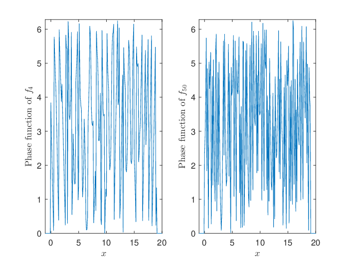
Fig. II.2: (a) The phase function θ​(f4​(x))\theta(f_{4}(x)) of f4f_{4}; (b) The phase function θ​(f50​(x))\theta(f_{50}(x)) of f50f_{50}.

Refer to caption

Fig. II.3: (a) The CDF of Error​(f4)\hbox{Error}(f_{4}) in the noiseless setting; (b) The CDF of Error​(f50)\hbox{Error}(f_{50}) in the noiseless setting.
SNR 50 60 70 80 90 100 110 120 130
f4f_{4} 0.0070 0.0940 0.2800 0.4830 0.6440 0.7990 0.8860 0.9410 0.9970
f50f_{50} 0.0240 0.1770 0.4040 0.6270 0.7330 0.8430 0.9090 0.9520 0.9880
TABLE II.1: Success rate vs noise level (SNR).

This section is to verify Theorem II.5. Our test SIS Vca​(ϕa,b,p)V_{\hbox{ca}}(\phi_{a,b,p}) is related with [34, section 6.3.1]. Specifically,

ϕa,b,p​(x)=23​2​π​|b|​e−i​a​(x−2)22​b​e−i​p⁡(x−2)b​cos2⁡π⁡(x−2)4​χ(0,4)​(x).\displaystyle\begin{array}[]{lll}\phi_{a,b,p}(x)\\ =\frac{2}{3}\sqrt{2\pi|b|}e^{-\textbf{i}\frac{a(x-2)^{2}}{2b}}e^{-\textbf{i}\frac{p(x-2)}{b}}\cos^{2}\frac{\pi(x-2)}{4}\chi_{(0,4)}(x).\end{array}

By section I-C1, both ϕ4,0.8,1\phi_{4,0.8,1} and ϕ50,0.8,1\phi_{50,0.8,1} are GHC-generators. The test signal

fa​(x):=∑n=015cn​ϕa,0.8,1​(x−n),\displaystyle\begin{array}[]{lll}f_{a}(x):=\sum_{n=0}^{15}c_{n}\phi_{a,0.8,1}(x-n),\end{array}

where a=4,50a=4,50 and 𝒢⁡(fa)<3\mathcal{G}(f_{a})<3. See Fig. II.1 for their graphs. In Fig. II.2 we also plot the phase function θ​(fa​(x))\theta(f_{a}(x)) defined via fa​(x)=|fa​(x)|​ei​θ​(fa​(x))f_{a}(x)=|f_{a}(x)|e^{\textbf{i}\theta(f_{a}(x))}. Clearly, the two signals are highly oscillatory. By Theorem II.5, fa​(x)f_{a}(x) can be determined with probability 11, up to a unimodular, by the random samples {|fa(t0)|}⋃{|fa(n+tn1)|,|fa(n+tn2)|,|fa(n+tn3)|:n=1,…,18},\{|f_{a}(t_{0})|\}\bigcup\{|f_{a}(n+t_{n_{1}})|,|f_{a}(n+t_{n_{2}})|,|f_{a}(n+t_{n_{3}})|:n=1,\ldots,18\}, where t0,tn1,tn2,tn3∼U​(0,1)t_{0},t_{n_{1}},t_{n_{2}},t_{n_{3}}\sim\textbf{U}(0,1). In the noiseless setting, 10310^{3} trials are conducted to determine fa​(x)f_{a}(x) by Approach II-B. The error is defined as

Error​(fa):=log10⁡(minγ∈(0,2​π]⁡‖{ck}−ei​γ​{c~k}‖2/‖{ck}‖2),\displaystyle\begin{array}[]{lll}\hbox{Error}(f_{a})\\ :=\log_{10}(\min_{\gamma\in(0,2\pi]}||\{c_{k}\}-e^{\textbf{i}\gamma}\{\widetilde{c}_{k}\}||_{2}/||\{c_{k}\}||_{2}),\end{array}

where {c~k}\{\widetilde{c}_{k}\} is the coefficient sequence of the reconstruction version f~a​(x)=∑n=015c~n​ϕa,0.8,1​(x−n)\widetilde{f}_{a}(x)=\sum_{n=0}^{15}\widetilde{c}_{n}\phi_{a,0.8,1}(x-n). Approach II-B is considered to be successful if Error​(fa)≤−1.8\hbox{Error}(f_{a})\leq-1.8. The cumulative distribution function (CDF) of Error​(fa)\hbox{Error}(f_{a}) is defined as

CDF​(x)=#⁡(Error​(fa)≤x)103.\displaystyle\hbox{CDF}(x)=\frac{\#\big(\hbox{Error}(f_{a})\leq x\big)}{10^{3}}. (2.74)

Fig. II.3 confirms that with probability 11, the signals can be determined in the noiseless setting.

In what follows we examine the robustness of Approach II-B to noise corruption. The observed values of {|f(t0)|}∪{|f(n+tn1)|,|f(n+tn2)|,|f(n+tn3)|:n=1,…,18}\{|f(t_{0})|\}\cup\{|f(n+t_{n_{1}})|,|f(n+t_{n_{2}})|,|f(n+t_{n_{3}})|:n=1,\ldots,18\} in a trial are denoted by {|f(t^0)|}∪{|f(n+t^n1)|,|f(n+t^n2)|,|f(n+t^n3)|:n=1,…,18}\{|f(\widehat{t}_{0})|\}\cup\{|f(n+\widehat{t}_{n_{1}})|,|f(n+\widehat{t}_{n_{2}})|,|f(n+\widehat{t}_{n_{3}})|:n=1,\ldots,18\}. We add the Gaussian noise ε∼N​(0,σ2)\varepsilon\sim\textbf{N}(0,\sigma^{2}) to the noiseless samples. That is, we employ the noisy samples {|fa(t^0)|+ε}∪{|fa(n+t^n1)|+ε,|fa(n+t^n2)|+ε,|fa(n+t^n3)|+ε:n=1,…,18}\{|f_{a}(\widehat{t}_{0})|+\varepsilon\}\cup\{|f_{a}(n+\widehat{t}_{n_{1}})|+\varepsilon,|f_{a}(n+\widehat{t}_{n_{2}})|+\varepsilon,|f_{a}(n+\widehat{t}_{n_{3}})|+\varepsilon:n=1,\ldots,18\} to conduct Approach II-B. The variance σ2\sigma^{2} is chosen such that the desired signal to noise ratio (SNR) is expressed by

SNR=10​log10⁡(‖Fa‖2255​σ2),\displaystyle\begin{array}[]{lllllllllllllllll}\hbox{SNR}=10\log_{10}\big(\frac{||\textbf{F}_{a}||^{2}_{2}}{55\sigma^{2}}\big),\end{array}

where ‖Fa‖22=|fa​(t^0)|2+∑k=13∑n=118|fa​(n+t^nk)|2||\textbf{F}_{a}||^{2}_{2}=|f_{a}(\widehat{t}_{0})|^{2}+\sum^{3}_{k=1}\sum^{18}_{n=1}|f_{a}(n+\widehat{t}_{n_{k}})|^{2}. In the noisy setting, 10310^{3} trials are also conducted to reconstruct f4​(x)f_{4}(x) and f50​(x)f_{50}(x), respectively. Their reconstruction success rates (CDF​(−1.8)\hbox{CDF}(-1.8)) are recorded in Table II.1.

III Random phaseless sampling of causal and real-valued signals in real-generated SISs

Throughout this section, let φ\varphi be a real-valued GHC-generator such that supp​(φ)⊆(0,s)\hbox{supp}(\varphi)\subseteq(0,s) with the integer s≥2s\geq 2. This section focuses on the PLS of real-valued signals in

Vca(φ)={∑∞k=0ckφ(⋅−k):{ck∈ℝ}∈ℓ2,c0≠0}.\displaystyle\begin{array}[]{lll}V_{\hbox{ca}}(\varphi)=\big\{\sum^{\infty}_{k=0}c_{k}\varphi(\cdot-k):\{c_{k}\in\mathbb{R}\}\in\ell^{2},c_{0}\neq 0\big\}.\end{array}

Some denotations and definitions are helpful for discussion. Suppose that the signal f∈Vca​(φ)f\in V_{\hbox{ca}}(\varphi) is denoted by

f=∑k=0∞ckφ(⋅−k).\displaystyle\begin{array}[]{lll}f=\sum_{k=0}^{\infty}c_{k}\varphi(\cdot-k).\end{array}

As in section II-B denote 𝒩f=sup{k:ck≠0}\mathcal{N}_{f}=\sup\{k:c_{k}\neq 0\}. As in (II-B), define the index set InI_{n} by

In={{0,1,…,n−1},1≤n≤s−1,{n−s+1,…,n−1},n≥s.\displaystyle I_{n}=\left\{\begin{array}[]{lll}\{0,1,\ldots,n-1\},&1\leq n\leq s-1,\\ \{n-s+1,\ldots,n-1\},&n\geq s.\end{array}\right.

For n≥1n\geq 1 and the signal ff in (III), define an auxiliary function

vℜn,f(x):=∑k∈Inckφ(n+x−k),x∈(0,1).\displaystyle\begin{array}[]{lll}v^{\Re}_{n,f}(x):=\sum_{k\in I_{n}}c_{k}\varphi(n+x-k),x\in(0,1).\end{array}

Moreover, define

Aℜn,f(x,y):=|f|​(n+x)|φ|2​(x)[φ(x)φ(y)vℜn,f(y)−vℜn,f(x)φ2(y)],\displaystyle\begin{array}[]{lll}A^{\Re}_{n,f}(x,y):=\frac{|f|(n+x)}{|\varphi|^{2}(x)}\Big[\varphi(x)\varphi(y)v^{\Re}_{n,f}(y)\\ \quad\quad\quad\quad\quad\quad\quad\quad\quad\quad-v^{\Re}_{n,f}(x)\varphi^{2}(y)\Big],\end{array}

and

Cn,fℜ​(x,y):=|f|2​(n+y)−|vn,fℜ|2​(y)+2​vn,fℜ​(x)​vn,fℜ​(y)​φ​(y)φ⁡(x)−|φ|2​(y)|φ|2​(x)​[|f|2​(n+x)+|vn,fℜ|2​(x)],\displaystyle\begin{array}[]{lll}C^{\Re}_{n,f}(x,y)&:=|f|^{2}(n+y)-|v^{\Re}_{n,f}|^{2}(y)\\ &+\frac{2v^{\Re}_{n,f}(x)v^{\Re}_{n,f}(y)\varphi(y)}{\varphi(x)}\\ &\ -\frac{|\varphi|^{2}(y)}{|\varphi|^{2}(x)}\Big[|f|^{2}(n+x)+|v^{\Re}_{n,f}|^{2}(x)\Big],\end{array}

whenever x,y∈(0,1)x,y\in(0,1) such that φ⁡(x)≠0\varphi(x)\neq 0. The maximum gap 𝒢f\mathcal{G}_{f} is defined via Definition II.8 with ϕ\phi replaced by φ.\varphi. The sign function sgn​(x)\hbox{sgn}(x) takes 1,−11,-1 and 00 when x>0,x<0x>0,x<0 and x=0,x=0, respectively.

Refer to caption

Fig. III.4: (a) The graph of f10,−0.2381,1f_{10,-0.2381,1}; (b) The graph of the phase function of f10,−0.2381,1f_{10,-0.2381,1}; (c) The graph of f50,−0.2381,1f_{50,-0.2381,1}; (d) The graph of the phase function of f50,−0.2381,1f_{50,-0.2381,1}; (e) The graph of f10−6,−0.0038,0f_{10^{-6},-0.0038,0}; (f) The graph of the phase function of f10−6,−0.0038,0f_{10^{-6},-0.0038,0}.

Refer to caption

Fig. III.5: (a) The CDF of Error​(f10,−0.2381,1)\hbox{Error}(f_{10,-0.2381,1}) in the noiseless setting; (b) The CDF of Error​(f50,−0.2381,1)\hbox{Error}(f_{50,-0.2381,1}) in the noiseless setting; (c) The CDF of Error​(f10−6,−0.0038,0)\hbox{Error}(f_{10^{-6},-0.0038,0}) in the noiseless setting

Refer to caption

Fig. III.6: (a) The graph of A1,g10ℜ​(0.5,x)A^{\Re}_{1,g_{10}}(0.5,x); (b) The graph of A1,g50ℜ​(0.5,x)A^{\Re}_{1,g_{50}}(0.5,x)

III-A Random PLS of real-valued signals in Vca​(φ)V_{\hbox{ca}}(\varphi)

We next establish the main theorem of this section. It is the counterpart of Theorem II.5.

Theorem III.1

Let φ\varphi be a real-valued GHC-generator such that supp​(φ)⊆(0,s)\hbox{supp}(\varphi)\subseteq(0,s) with the integer s≥2s\geq 2. Then any nonseparable and real-valued signal f∈Vca​(φ)f\in V_{\hbox{ca}}(\varphi) can be determined (up to a sign) with probability 11 by the random samples {|f(t0)|}∪{|f(n+tn1)|,|f(n+tn2)|:n=1,…,∞}\{|f(t_{0})|\}\cup\{|f(n+t_{n_{1}})|,|f(n+t_{n_{2}})|:n=1,\ldots,\infty\}, where the i.i.d random variables {t0}∪{tn1,tn2:n=1,…,∞}∼U(0,1)\{t_{0}\}\cup\{t_{n_{1}},t_{n_{2}}:n=1,\ldots,\infty\}\sim\textbf{U}(0,1).

Proof:

Since ff is nonseparable, by the same argument as in Lemma II.9 we have 𝒢f<s−1\mathcal{G}_{f}<s-1, which together with φ\varphi being a real-valued GHC-generator leads to the probability P⁡(|f⁡(k+tki)|>0)=1P(|f(k+t_{k_{i}})|>0)=1 for any k∈{0,…,𝒩f+s−1}.k\in\{0,\ldots,\mathcal{N}_{f}+s-1\}. Clearly, P⁡(|φ⁡(tni)|>0)=1.P(|\varphi(t_{n_{i}})|>0)=1. As in section II-F, it is sufficient to prove that the phases {θ(f(t0))}∪{θ(f(n+tni)):n=1,…,𝒩f+s−1,i=1,2}\{\theta(f(t_{0}))\}\cup\{\theta(f(n+t_{n_{i}})):n=1,\ldots,\mathcal{N}_{f}+s-1,i=1,2\} can be determined, up to the constant π\pi, with probability 1.1.

Denote f=∑k=0∞ckφ(⋅−k).f=\sum_{k=0}^{\infty}c_{k}\varphi(\cdot-k). By the similar argument as in the proof of Lemma II.10, we can prove that

P(An,fℜ(tn1,tn2)≠0)=1,n=1,…,𝒩f+s−1.\displaystyle P(A^{\Re}_{n,f}(t_{n_{1}},t_{n_{2}})\neq 0)=1,n=1,\ldots,\mathcal{N}_{f}+s-1. (3.86)

Assume that z0=ei​θ​(f⁡(t0))∈{1,−1}z_{0}=e^{\textbf{i}\theta(f(t_{0}))}\in\{1,-1\} is assigned exactly. As previously, P⁡(|f⁡(n+tni)|>0)=P⁡(|φ⁡(tni)|>0)=1.P(|f(n+t_{n_{i}})|>0)=P(|\varphi(t_{n_{i}})|>0)=1. Then

f⁡(t0)=z0​|f⁡(t0)|,\displaystyle\begin{array}[]{lll}f(t_{0})=z_{0}|f(t_{0})|,\end{array}

and c0=z0​|f⁡(t0)|φ⁡(t0)c_{0}=\frac{z_{0}|f(t_{0})|}{\varphi(t_{0})} with probability 11. We next determine θ⁡(f⁡(t11+1))\theta(f(t_{1_{1}}+1)) and c1c_{1}. Similarly to (II-B), we have

{|v1,fℜ​(t11)+c1​φ​(t11)|=|f⁡(1+t11)|,|v1,fℜ​(t12)+c1​φ​(t12)|=|f⁡(1+t12)|.\displaystyle\left\{\begin{array}[]{lll}|v^{\Re}_{1,f}(t_{1_{1}})+c_{1}\varphi(t_{1_{1}})|=|f(1+t_{1_{1}})|,\\ |v^{\Re}_{1,f}(t_{1_{2}})+c_{1}\varphi(t_{1_{2}})|=|f(1+t_{1_{2}})|.\end{array}\right.

Denote f⁡(1+t11):=z1​|f⁡(1+t11)|f(1+t_{1_{1}}):=z_{1}|f(1+t_{1_{1}})| with z1∈{1,−1}z_{1}\in\{1,-1\} to be determined. By the similar argument as in (II-B), we can prove that z1z_{1} is the solution to

A1,fℜ​(t11,t12)​z2−C1,fℜ​(t11,t12)​z+A1,fℜ​(t11,t12)=0.\displaystyle\begin{array}[]{lll}A^{\Re}_{1,f}(t_{1_{1}},t_{1_{2}})z^{2}-C^{\Re}_{1,f}(t_{1_{1}},t_{1_{2}})z+A^{\Re}_{1,f}(t_{1_{1}},t_{1_{2}})=0.\end{array}

It follows from (3.86) that with probability 11, there exist at most two solutions to the above equation. Note that the product of the two solutions is 11. Then there exists a unique solution with the same probability. More precisely,

z1=sgn​(C1,fℜ​(t11,t12)A1,fℜ​(t11,t12)).\displaystyle\begin{array}[]{lll}z_{1}=\hbox{sgn}\big(\frac{C^{\Re}_{1,f}(t_{1_{1}},t_{1_{2}})}{A^{\Re}_{1,f}(t_{1_{1}},t_{1_{2}})}\big).\end{array}

Therefore under the assumption (III-A), c1=z1​|f⁡(1+t11)|−v1,f​(t11)φ⁡(t11)c_{1}=\frac{z_{1}|f(1+t_{1_{1}})|-v_{1,f}(t_{1_{1}})}{\varphi(t_{1_{1}})} with probability 11. And θ⁡(f⁡(1+t1i))\theta(f(1+t_{1_{i}})) can be determined with probability 11. Continuing the above procedures, {θ(f(t0))}∪{θ(f(n+tni)):n=1,…,𝒩f+s−1,i=1,2}\{\theta(f(t_{0}))\}\cup\{\theta(f(n+t_{n_{i}})):n=1,\ldots,\mathcal{N}_{f}+s-1,i=1,2\} can be determined with the same probability.

Contrary to (III-A), we next assign

f⁡(t0)=−z0​|f⁡(t0)|.\displaystyle\begin{array}[]{lll}f(t_{0})=-z_{0}|f(t_{0})|.\end{array}

Under (III-A), we shall prove that {θ(f(t0))+π}∪{θ(f(n+tni))+π:n=1,…,𝒩f+s−1,i=1,2}\{\theta(f(t_{0}))+\pi\}\cup\{\theta(f(n+t_{n_{i}}))+\pi:n=1,\ldots,\mathcal{N}_{f}+s-1,i=1,2\} or f~=∑k=0∞c~kφ(⋅−k)\widetilde{f}=\sum_{k=0}^{\infty}\widetilde{c}_{k}\varphi(\cdot-k) can be determined with probability 11, where c~k=−ck\widetilde{c}_{k}=-c_{k}. First it follows from P⁡(|φ⁡(t0)|≠0)=1P(|\varphi(t_{0})|\neq 0)=1 that

c~0=−z0​|f⁡(t0)|φ⁡(t0)=−c0.\displaystyle\begin{array}[]{lll}\widetilde{c}_{0}=-\frac{z_{0}|f(t_{0})|}{\varphi(t_{0})}=-c_{0}.\end{array}

Then θ⁡(f~​(t0i))=θ⁡(f⁡(t0i))+π\theta(\widetilde{f}(t_{0_{i}}))=\theta(f(t_{0_{i}}))+\pi. By (III), (III) and (III-A), we have A1,f~ℜ​(t11,t12)=−A1,fℜ​(t11,t12)A^{\Re}_{1,\widetilde{f}}(t_{1_{1}},t_{1_{2}})=-A^{\Re}_{1,f}(t_{1_{1}},t_{1_{2}}) and C1,f~ℜ​(t11,t12)=C1,fℜ​(t11,t12)C^{\Re}_{1,\widetilde{f}}(t_{1_{1}},t_{1_{2}})=C^{\Re}_{1,f}(t_{1_{1}},t_{1_{2}}). Moreover, as in (III-A), sgn​(f~​(1+t11))\hbox{sgn}(\widetilde{f}(1+t_{1_{1}})) is the solution to

A1,f~ℜ​(t11,t12)​z2−C1,f~ℜ​(t11,t12)​z+A1,f~ℜ​(t11,t12)=0.\displaystyle\begin{array}[]{lll}A^{\Re}_{1,\widetilde{f}}(t_{1_{1}},t_{1_{2}})z^{2}-C^{\Re}_{1,\widetilde{f}}(t_{1_{1}},t_{1_{2}})z+A^{\Re}_{1,\widetilde{f}}(t_{1_{1}},t_{1_{2}})=0.\end{array}

As in (III-A), the solution is given by

z=sgn​(C1,f~ℜ​(t11,t12)A1,f~ℜ​(t11,t12))=−sgn​(C1,fℜ​(t11,t12)A1,fℜ​(t11,t12)).\displaystyle\begin{array}[]{lll}z=\hbox{sgn}\big(\frac{C^{\Re}_{1,\widetilde{f}}(t_{1_{1}},t_{1_{2}})}{A^{\Re}_{1,\widetilde{f}}(t_{1_{1}},t_{1_{2}})}\big)=-\hbox{sgn}\big(\frac{C^{\Re}_{1,f}(t_{1_{1}},t_{1_{2}})}{A^{\Re}_{1,f}(t_{1_{1}},t_{1_{2}})}\big).\end{array}

Then θ⁡(f~​(1+t11))=θ⁡(f⁡(1+t11))+π\theta(\widetilde{f}(1+t_{1_{1}}))=\theta(f(1+t_{1_{1}}))+\pi. Consequently, c~1=−c1\widetilde{c}_{1}=-c_{1} and θ⁡(f~​(1+t12))=θ⁡(f⁡(1+t12))+π\theta(\widetilde{f}(1+t_{1_{2}}))=\theta(f(1+t_{1_{2}}))+\pi. By recursion on nn, we can prove that {θ(f(t0))+π}∪{θ(f(n+tni))+π:n=1,…,𝒩f+s−1,i=1,2}\{\theta(f(t_{0}))+\pi\}\cup\{\theta(f(n+t_{n_{i}}))+\pi:n=1,\ldots,\mathcal{N}_{f}+s-1,i=1,2\} can be determined with probability 1.1. ∎

The following proposition concerns on the local reconstruction. It is the counterpart of Proposition II.6.

Proposition III.2

Let φ\varphi and ff be as in Theorem III.1. Then for any integer L>1L>1, the restriction f[0,L]f_{[0,L]} of ff on [0,L][0,L] can be determined with probability 11, up to a sign, by the random samples {|f(t0)|}∪{|f(n+tn1)|,|f(n+tn2)|:n=1,…,L−1}\{|f(t_{0})|\}\cup\{|f(n+t_{n_{1}})|,|f(n+t_{n_{2}})|:n=1,\ldots,L-1\}, where the i.i.d random variables {t0}∪{tn1,tn2:n=1,…,L−1}∼U(0,1)\{t_{0}\}\cup\{t_{n_{1}},t_{n_{2}}:n=1,\ldots,L-1\}\sim\textbf{U}(0,1).

Proof:

The proof is based on that of Theorem III.1. And it can be concluded by the similar argument as in section II-G. ∎

III-B PD-CR for nonseparable real-valued signals in Vca​(φ)V_{\hbox{ca}}(\varphi)

Let {t^0}∪{t^n1,t^n2:n=1,…,∞}\{\widehat{t}_{0}\}\cup\{\widehat{t}_{n_{1}},\widehat{t}_{n_{2}}:n=1,\ldots,\infty\} be the observed values of random variables {t0}∪{tn1,tn2:n=1,…,∞}\{t_{0}\}\cup\{t_{n_{1}},t_{n_{2}}:n=1,\ldots,\infty\} in Theorem III.1. Based on the proof of Theorem III.1, in what follows we establish an approach for the PLS of nonseparable real-valued signals in Vca​(φ)V_{\hbox{ca}}(\varphi).

Approach III-B

Input: Samples {|f(t^0)|}∪{|f(k+t^kj)|:j=1,2,k=1,…,n}\{|f(\widehat{t}_{0})|\}\cup\{|f(k+\widehat{t}_{k_{j}})|:j=1,2,k=1,\ldots,n\} where t^0,t^kj∈(0,1)\widehat{t}_{0},\widehat{t}_{k_{j}}\in(0,1) and n≤𝒩f+s−1n\leq\mathcal{N}_{f}+s-1. Assign initial phase θ⁡(f⁡(t^0))=θ~0∈{0,π}\theta(f(\widehat{t}_{0}))=\widetilde{\theta}_{0}\in\{0,\pi\}; c0=ei​θ~0​|f⁡(t^0)|/φ⁡(t^0)c_{0}=e^{\textbf{i}\widetilde{\theta}_{0}}|f(\widehat{t}_{0})|/\varphi(\widehat{t}_{0}).

Output: {ck}k=0n\{c_{k}\}^{n}_{k=0} and {θ(f(t^0))}∪{θ(f(k+t^kj)):j=1,2,k=1,…,n}\{\theta(f(\widehat{t}_{0}))\}\cup\{\theta(f(k+\widehat{t}_{k_{j}})):j=1,2,k=1,\ldots,n\}.

Recursion assumption: Assume that the phases {θ(f(k+t^kj)):j=1,2,k=1,…,n−1}\{\theta(f(k+\widehat{t}_{k_{j}})):j=1,2,k=1,\ldots,n-1\} and coefficients {ck}k=0n−1\{c_{k}\}^{n-1}_{k=0} have been recovered. Then {θ(f(n+t^nj)):j=1,2}\{\theta(f(n+\widehat{t}_{n_{j}})):j=1,2\} and cnc_{n} are recovered by the following steps:

step 1: Compute vn,fℜ​(t^n1)v^{\Re}_{n,f}(\widehat{t}_{n_{1}}), An,fℜ​(t^n1,t^n2)A^{\Re}_{n,f}(\widehat{t}_{n_{1}},\widehat{t}_{n_{2}}) and Cn,fℜ​(t^n1,t^n2)C^{\Re}_{n,f}(\widehat{t}_{n_{1}},\widehat{t}_{n_{2}}) by (III), (III) and (III), respectively.

step 2: θ⁡(f⁡(n+t^n1))∈{0,π}\theta(f(n+\widehat{t}_{n_{1}}))\in\{0,\pi\} is recovered by computing ei​θ​(f⁡(n+t^n1))=sgn​(Cn,fℜ​(t^n1,t^n2)An,fℜ​(t^n1,t^n2))e^{\textbf{i}\theta(f(n+\widehat{t}_{n_{1}}))}=\hbox{sgn}\big(\frac{C^{\Re}_{n,f}(\widehat{t}_{n_{1}},\widehat{t}_{n_{2}})}{A^{\Re}_{n,f}(\widehat{t}_{n_{1}},\widehat{t}_{n_{2}})}\big). And cn=[ei​θ​(f⁡(n+t^n1))​|f⁡(n+t^n1)|−vn,fℜ​(t^n1)]/φ⁡(t^n1)c_{n}=[e^{\textbf{i}\theta(f(n+\widehat{t}_{n_{1}}))}|f(n+\widehat{t}_{n_{1}})|-v^{\Re}_{n,f}(\widehat{t}_{n_{1}})]/\varphi(\widehat{t}_{n_{1}}).

III-C Numerical simulation: costing small number of samples to reconstruct highly oscillatory real-valued chirps

SNR 35 40 50 60 70 80 90 100
f50,−0.2381,1f_{50,-0.2381,1} 0.0100 0.0590 0.2460 0.5290 0.6870 0.8450 0.9200 0.9620
f10,−0.2381,1f_{10,-0.2381,1} 0.0160 0.0470 0.2520 0.4590 0.6570 0.8540 0.9090 0.9560
f10−6,−0.0038,0f_{10^{-6},-0.0038,0} 0.1100 0.3370 0.7390 0.9080 0.9520 0.9800 0.9850 0.9960
TABLE III.2: Success rate vs noise level (SNR).

This section is to examine the efficiency of Approach III-B. The generator φ\varphi is chosen as ϕa,b,p,ℜ\phi_{a,b,p,\Re}, the real part of ϕa,b,p\phi_{a,b,p} defined in section II-H. The test signal is

fa,b,p​(t)=∑n=015cn,a​ϕa,b,p,ℜ​(t−n),\displaystyle\begin{array}[]{lll}f_{a,b,p}(t)=\sum_{n=0}^{15}c_{n,a}\phi_{a,b,p,\Re}(t-n),\end{array}

where c0,a≠0,cn,a∈ℝc_{0,a}\neq 0,c_{n,a}\in\mathbb{R}. It is easy to check that fa,b,p​(t)f_{a,b,p}(t) can be rewritten as the real-valued chirp form (c.f. [40]): A⁡(t)​cos⁡(λ​υ​(t))A(t)\cos(\lambda\upsilon(t)) with A⁡(⋅)≥0A(\cdot)\geq 0. By the analysis in section I-C2, we can check that ϕ10,−0.238,1,ℜ\phi_{10,-0.238,1,\Re}, ϕ50,−0.238,1,ℜ\phi_{50,-0.238,1,\Re} and ϕ10−6,−0.0038,0,ℜ\phi_{10^{-6},-0.0038,0,\Re} are all real-valued GHC-generators. We choose f10,−0.2381,1f_{10,-0.2381,1}, f50,−0.2381,1f_{50,-0.2381,1} and f10−6,−0.0038,0f_{10^{-6},-0.0038,0} as test signals. Their graphs are plotted in Fig. III.4 (a, c, e). Moreover, the phase function θ​(fa,b,p​(x))\theta(f_{a,b,p}(x)), taking 00 and π\pi when fa,b,p​(x)≥0f_{a,b,p}(x)\geq 0 and fa,b,p​(x)<0f_{a,b,p}(x)<0, respectively, is plotted in Fig. III.4 (b, d, f).

Fig. III.4 (b, d, f) imply that f10,−0.2381,1f_{10,-0.2381,1} and f50,−0.2381,1f_{50,-0.2381,1} are much more oscillatory than f10−6,−0.0038,0f_{10^{-6},-0.0038,0}. It should be noted that a great number of deterministic samples are necessary for the local reconstructions of f10,−0.2381,1f_{10,-0.2381,1} and f50,−0.2381,1f_{50,-0.2381,1}. To make this point, define

ga​(t)=∑n=01cn,a​ϕa,−0.238,1,ℜ​(t−n),t∈(0,2),\displaystyle g_{a}(t)=\sum_{n=0}^{1}c_{n,a}\phi_{a,-0.238,1,\Re}(t-n),\ t\in(0,2), (3.97)

where c0,10=0.7064,c1,10=−0.6183,c0,50=−0.5874c_{0,10}=0.7064,c_{1,10}=-0.6183,c_{0,50}=-0.5874 and c1,50=0.2659c_{1,50}=0.2659 are as in (III-C). Clearly,

ga​(t)=fa,−0.2381,1​(t),t∈(0,2),\displaystyle g_{a}(t)=f_{a,-0.2381,1}(t),\ t\in(0,2), (3.98)

and the reconstruction of gag_{a} is equivalent to ones of c0,ac_{0,a} and c1,ac_{1,a}. Suppose that c0,ac_{0,a} and c1,ac_{1,a} can be recovered by any L̊\mathring{L} deterministic samples {|ga(t^0)|,|ga(1+t^1i)|:i=1,…,L̊−1}\{|g_{a}(\widehat{t}_{0})|,|g_{a}(1+\widehat{t}_{1_{i}})|:i=1,\ldots,\mathring{L}-1\}, where t^0\widehat{t}_{0}, t^1i∈(0,1)\widehat{t}_{1_{i}}\in(0,1). We next estimate L̊.\mathring{L}. It is required that ϕa,−0.238,1,ℜ​(t^0)≠0\phi_{a,-0.238,1,\Re}(\widehat{t}_{0})\neq 0 such that c0,ac_{0,a} can be determined, up to a sign, by |ga​(t^0)||g_{a}(\widehat{t}_{0})|. Otherwise, |ga​(t^0)||g_{a}(\widehat{t}_{0})| is useless for determining c0,ac_{0,a}. Without loss of generality, assume that c0,ac_{0,a} is determined and |ga​(1+t^1i)|≠0.|g_{a}(1+\widehat{t}_{1_{i}})|\neq 0. Next we need to determine c1,ac_{1,a}. Then the determination of c1,ac_{1,a} is equivalent to the determination of z:=sgn​(ga​(1+t^11))z:=\hbox{sgn}(g_{a}(1+\widehat{t}_{1_{1}})). By the analysis in (III-A), zz is the solution to (III-A) with A1,fℜ​(t11,t12)A^{\Re}_{1,f}(t_{1_{1}},t_{1_{2}}) and C1,fℜ​(t11,t12)C^{\Re}_{1,f}(t_{1_{1}},t_{1_{2}}) therein replaced by A1,gaℜ​(t^11,t^1j)A^{\Re}_{1,g_{a}}(\widehat{t}_{1_{1}},\widehat{t}_{1_{j}}) and C1,gaℜ​(t^11,t^1j)C^{\Re}_{1,g_{a}}(\widehat{t}_{1_{1}},\widehat{t}_{1_{j}}), respectively, where j≠1j\neq 1. Clearly, zz can be determined if and only if A1,gaℜ​(t^11,t^1j)≠0A^{\Re}_{1,g_{a}}(\widehat{t}_{1_{1}},\widehat{t}_{1_{j}})\neq 0. As an example, we choose t^11=0.5\widehat{t}_{1_{1}}=0.5 without bias. See the graph of A1,gaℜ​(0.5,x)A^{\Re}_{1,g_{a}}(0.5,x) on (0,1)(0,1) in Fig. III.6. Obviously the number of zeros of A1,gaℜ​(0.5,x)A^{\Re}_{1,g_{a}}(0.5,x) on (0,1)(0,1) is much larger than 22. Especially, we found that the number of zeros of A1,g50ℜ​(0.5,x)A^{\Re}_{1,g_{50}}(0.5,x) is not smaller than 256.\textbf{256}. Then we need at least 257 additional deterministic samples on (1,2)(1,2) to avoid A1,g50ℜ​(0.5,x)=0.A^{\Re}_{1,g_{50}}(0.5,x)=0. Therefore for reconstructing g50g_{50}, L̊≥259\mathring{L}\geq\textbf{259} although it is determined by only two coefficients. By Proposition III.2, however, gag_{a} can be determined, with probability 11, by just three random samples. Allowing for (3.98) we just need to check the recovery efficiency of fa,−0.2381,1f_{a,-0.2381,1}.

In the present simulation, by the random samples

{|fa,b,p(t0)|}∪{|fa,b,p(n+tn1)|,|fa,b,p(n+tn2)|:n=1,…,18},\displaystyle\begin{array}[]{lll}\{|f_{a,b,p}(t_{0})|\}\cup\{|f_{a,b,p}(n+t_{n_{1}})|,|f_{a,b,p}(n+t_{n_{2}})|:\\ \quad n=1,\ldots,18\},\end{array}

10310^{3} trials of Approach III-B are conducted to recover fa,b,pf_{a,b,p}, where {t0}∪{tn1,tn2:n=1,…,18}∼U(0,1)\{t_{0}\}\cup\{t_{n_{1}},t_{n_{2}}:n=1,\ldots,18\}\sim\textbf{U}(0,1). The recovery error is defined as

Error​(fa,b,p):=log10(minγ∈{1,−1}||{ck,a}−γ{c~k,a}||2/||{ck,a}||2),\displaystyle\begin{array}[]{lll}\hbox{Error}(f_{a,b,p})&:=\log_{10}(\min_{\gamma\in\{1,-1\}}||\{c_{k,a}\}\\ &\quad\quad\quad\quad-\gamma\{\widetilde{c}_{k,a}\}||_{2}/||\{c_{k,a}\}||_{2}),\end{array}

where {c~k,a}\{\widetilde{c}_{k,a}\} is the recovery version of {ck,a}.\{c_{k,a}\}. As in section II-H, the approach is considered successful if Error​(fa,b,p)≤−1.8\hbox{Error}(f_{a,b,p})\leq-1.8, and the cumulative distribution function (CDF) of the error is defined via (2.74). Clearly, Fig. III.5 implies that f10,−0.2381,1f_{10,-0.2381,1}, f50,−0.2381,1f_{50,-0.2381,1} and f10−6,−0.0038,0f_{10^{-6},-0.0038,0} can be recovered perfectly in the noiseless setting. To check the stability to noise, we also conduct 10310^{3} trials in the noisy setting. As in section II-H, we add the Gaussian noise ε∼N​(0,σ2)\varepsilon\sim\textbf{N}(0,\sigma^{2}) to the observed noiseless samples in (III-C). The variance σ2\sigma^{2} is chosen via (II-H) with 5555 therein replaced by 3737 such that the desired SNR can be expressed. As in the noiseless case, 10310^{3} trials are also conducted. The success rates (CDF​(−1.8)\hbox{CDF}(-1.8)) are recorded in Table III.2.

Comparing Table II.1 and Table III.2 we found that, for the low SNR (e.g. ≤60\leq 60), the stability to noise in the present simulation (real-valued case) is much stronger than that in section III-C (complex-valued case). We next interpret this from the phase distribution perspective.

Remark III.3

For a real-valued signal f∈V⁡(φ)f\in V(\varphi), its phase function θ⁡(f⁡(x))\theta(f(x)) has only two values: 00 and π\pi. Since the samples in (III-C) are perturbed, unavoidably so is Cn,fℜ​(t^n1,t^n2)An,fℜ​(t^n1,t^n2)\frac{C^{\Re}_{n,f}(\widehat{t}_{n_{1}},\widehat{t}_{n_{2}})}{A^{\Re}_{n,f}(\widehat{t}_{n_{1}},\widehat{t}_{n_{2}})} in step 2 of Approach II-B. If the perturbation ϵ\epsilon of Cn,fℜ​(t^n1,t^n2)An,fℜ​(t^n1,t^n2)\frac{C^{\Re}_{n,f}(\widehat{t}_{n_{1}},\widehat{t}_{n_{2}})}{A^{\Re}_{n,f}(\widehat{t}_{n_{1}},\widehat{t}_{n_{2}})} satisfies |ϵ|<|Cn,fℜ​(t^n1,t^n2)An,fℜ​(t^n1,t^n2)||\epsilon|<|\frac{C^{\Re}_{n,f}(\widehat{t}_{n_{1}},\widehat{t}_{n_{2}})}{A^{\Re}_{n,f}(\widehat{t}_{n_{1}},\widehat{t}_{n_{2}})}|, then θ⁡(f⁡(n+t^n1))\theta(f(n+\widehat{t}_{n_{1}})) can be decoded exactly through step 2. Unlike the real-valued case, Fig. II.2 implies that the phases of the complex-valued signals in section II-H are much more complicated. Therefore, it is no wonder that the stability in the present simulation is much stronger than that in section II-H.

On the other hand, it follows from Fig. III.4 (b, d, f) that the phase function of f10−6,−0.0038,0f_{10^{-6},-0.0038,0} varies much more slowly than those of f10,−0.2381,1f_{10,-0.2381,1} and f50,−0.2381,1f_{50,-0.2381,1}. And when SNR (≤50\leq 50) is low, numerical results in Table III.2 imply the much stronger stability for f10−6,−0.0038,0f_{10^{-6},-0.0038,0}.

Recall that the distribution and oscillation of the phase is the intrinsic property of a signal. Overall, the simulation results in section II-H and in the present section imply that the recovery stability to noise is related with the property.

IV Conclusion

We prove that the full spark property is not sufficient for the phaseless sampling in complex-generated shift-invariant spaces (SISs) (Theorem I.1). We establish a condition for decoding the phases of the samples (Theorem II.4). Based on Theorem II.4, we establish a reconstruction scheme in Approach II-B. Based on Approach II-B and the generalized Haar condition (GHC), nonseparable and causal (NC) signals in the complex-generated SISs can be determined with probability 11 if the random sampling density (SD) is not smaller than 33 (Theorem II.5). Approach II-B is modified to Approach III-B such that it is more adaptive to real-valued NC signals in real-generated SISs. Based on Approach III-B and GHC, real-valued NC signals in the real-generated SISs can be determined with probability 11 if the random SD is not smaller than 22 (Theorem III.1). Propositions II.6 and III.2 imply that the highly oscillatory signals can be determined locally, with probability 11, by a very small number of random samples.

V Appendix

V-A Proof of Lemma II.10

Since tn1,tn2t_{n_{1}},t_{n_{2}} and tn3t_{n_{3}} are i.i.d random variables, we just need to prove P⁡(An,f​(tn1,tn2)+Bn,f​(tn1,tn2)​i≠0)=1P\big(A_{n,f}(t_{n_{1}},t_{n_{2}})+B_{n,f}(t_{n_{1}},t_{n_{2}})\textbf{i}\neq 0\big)=1.

Define an event 𝔈~n,0:={ϕ(tn1)f¯(n+tn1)≠0}\widetilde{\mathfrak{E}}_{n,0}:=\{\phi(t_{n_{1}})\bar{f}(n+t_{n_{1}})\neq 0\} w.r.t tn1t_{n_{1}}. By (2.22), we have

𝔈~n,0={ϕ(tn1)(v¯n,f(tn1)+c¯nϕ¯(tn1))≠0}={∑k∈Inc¯kϕ(tn1)ϕ¯(n+tn1−k)+c¯n|ϕ|2(tn1)≠0}.\displaystyle\begin{array}[]{lll}\widetilde{\mathfrak{E}}_{n,0}\\ =\{\phi(t_{n_{1}})(\bar{v}_{n,f}(t_{n_{1}})+\bar{c}_{n}\bar{\phi}(t_{n_{1}}))\neq 0\}\\ =\{\sum_{k\in I_{n}}\bar{c}_{k}\phi(t_{n_{1}})\bar{\phi}(n+t_{n_{1}}-k)+\bar{c}_{n}|\phi|^{2}(t_{n_{1}})\neq 0\}.\end{array}

First, it is easy to derive from Lemma II.9 and the definition of 𝒩f\mathcal{N}_{f} that, for every n∈{1,2,…,𝒩f+s−1}n\in\{1,2,\ldots,\mathcal{N}_{f}+s-1\} there exists a nonzero coefficient in {ck:k∈In}\{c_{k}:k\in I_{n}\}. Moreover, Λϕ,2\Lambda_{\phi,2} in Proposition II.1 satisfies GHC. Then

μ({t∈(0,1):∑k∈Inc¯kϕ(t)ϕ¯(n+t−k)+c¯n|ϕ|2(t)=0})=0.\displaystyle\begin{array}[]{lll}\mu\Big(\{t\in(0,1):\sum_{k\in I_{n}}\bar{c}_{k}\phi(t)\bar{\phi}(n+t-k)\\ \quad\quad\quad\quad\quad\quad\quad+\bar{c}_{n}|\phi|^{2}(t)=0\}\Big)\\ =0.\end{array}

Therefore P⁡(𝔈~n,0)=1P(\widetilde{\mathfrak{E}}_{n,0})=1. Consequently, P⁡(𝔈n,0)=1P(\mathfrak{E}_{n,0})=1 where 𝔈n,0={|f⁡(n+tn1)||ϕ|2​(tn1)≠0}\mathfrak{E}_{n,0}=\big\{\frac{|f(n+t_{n_{1}})|}{|\phi|^{2}(t_{n_{1}})}\neq 0\big\}. Define an auxiliary (random) function w.r.t tn1t_{n_{1}} and tn2t_{n_{2}} by

an,f​(tn1,tn2)+bn,f​(tn1,tn2)​i:=ϕ¯​(tn1)​ϕ​(tn2)​v¯n,f​(tn2)−v¯n,f​(tn1)​|ϕ|2​(tn2).\displaystyle\begin{array}[]{lll}a_{n,f}(t_{n_{1}},t_{n_{2}})+b_{n,f}(t_{n_{1}},t_{n_{2}})\textbf{i}\\ :=\bar{\phi}(t_{n_{1}})\phi(t_{n_{2}})\bar{v}_{n,f}(t_{n_{2}})-\bar{v}_{n,f}(t_{n_{1}})|\phi|^{2}(t_{n_{2}}).\end{array}

Direct observation on (II-B) leads to that

An,f​(tn1,tn2)+Bn,f​(tn1,tn2)​i=|f|​(n+tn1)|ϕ|2​(tn1)​(an,f​(tn1,tn2)+bn,f​(tn1,tn2)​i).\displaystyle\begin{array}[]{lll}A_{n,f}(t_{n_{1}},t_{n_{2}})+B_{n,f}(t_{n_{1}},t_{n_{2}})\textbf{i}\\ =\frac{|f|(n+t_{n_{1}})}{|\phi|^{2}(t_{n_{1}})}\big(a_{n,f}(t_{n_{1}},t_{n_{2}})+b_{n,f}(t_{n_{1}},t_{n_{2}})\textbf{i}\big).\end{array}

As previously for every n∈{1,2,…,𝒩f}n\in\{1,2,\ldots,\mathcal{N}_{f}\}, there exists a nonzero coefficient in {ck:k∈In}\{c_{k}:k\in I_{n}\}. Then by (II-B) we have v¯n,f≢0.\bar{v}_{n,f}\not\equiv 0. Now it follows from Λϕ,2\Lambda_{\phi,2} in Proposition II.1 satisfying GHC that ϕ​v¯n,f\phi\bar{v}_{n,f} and |ϕ|2|\phi|^{2} are linearly independent, which together with P⁡(𝔈n,0)=1P(\mathfrak{E}_{n,0})=1 leads to an,f​(⋅,⋅)+bn,f​(⋅,⋅)​i≢0.a_{n,f}(\cdot,\cdot)+b_{n,f}(\cdot,\cdot)\textbf{i}\not\equiv 0. Then

1≥P⁡(an,f​(tn1,tn2)+bn,f​(tn1,tn2)​i≠0)≥P⁡(an,f​(tn1,tn2)+bn,f​(tn1,tn2)​i≠0|𝔈n,0)​P​(𝔈n,0)=P⁡(an,f​(tn1,tn2)+bn,f​(tn1,tn2)​i≠0|𝔈n,0)=1,\displaystyle\begin{array}[]{lll}1\geq P\big(a_{n,f}(t_{n_{1}},t_{n_{2}})+b_{n,f}(t_{n_{1}},t_{n_{2}})\textbf{i}\neq 0\big)\\ \ \ \geq P\big(a_{n,f}(t_{n_{1}},t_{n_{2}})+b_{n,f}(t_{n_{1}},t_{n_{2}})\textbf{i}\neq 0|\mathfrak{E}_{n,0}\big)P(\mathfrak{E}_{n,0})\\ \ \ =P\big(a_{n,f}(t_{n_{1}},t_{n_{2}})+b_{n,f}(t_{n_{1}},t_{n_{2}})\textbf{i}\neq 0|\mathfrak{E}_{n,0}\big)\\ \ \ =1,\end{array}

where Λϕ,2\Lambda_{\phi,2} satisfying GHC is used again in the last identity. The proof is concluded.

V-B Proof of Lemma II.11

If 0<|f|​(n+tn1)|ϕ|2​(tn1)<∞0<\frac{|f|(n+t_{n_{1}})}{|\phi|^{2}(t_{n_{1}})}<\infty, then it follows from (V-A) that θ⁡[An,f​(tn1,tn2)+Bn,f​(tn1,tn2)​i]\theta[A_{n,f}(t_{n_{1}},t_{n_{2}})+B_{n,f}(t_{n_{1}},t_{n_{2}})\textbf{i}] =θ⁡[an,f​(tn1,tn2)+bn,f​(tn1,tn2)​i]=\theta[a_{n,f}(t_{n_{1}},t_{n_{2}})+b_{n,f}(t_{n_{1}},t_{n_{2}})\textbf{i}], where an,f​(tn1,tn2)+bn,f​(tn1,tn2)​ia_{n,f}(t_{n_{1}},t_{n_{2}})+b_{n,f}(t_{n_{1}},t_{n_{2}})\textbf{i} is defined in (V-A). By direct calculation, for y∈(0,1)y\in(0,1) we have

ℜ⁡(an,f​(tn1,y)+i​bn,f​(tn1,y))=an,f​(tn1,y)=utn1,f​(ϕℜ2​(y)+ϕℑ2​(y))+∑k∈In[c~tn1,k,ℜ(ϕℜ(y)ϕℜ(y+n−k)+ϕℑ(y)ϕℑ(y+n−k))]−∑k∈In[c~tn1,k,ℑ(ϕℑ(y)ϕℜ(y+n−k)−ϕℜ(y)ϕℑ(y+n−k))],\displaystyle\begin{array}[]{lll}\Re(a_{n,f}(t_{n_{1}},y)+\textbf{i}b_{n,f}(t_{n_{1}},y))\\ =a_{n,f}(t_{n_{1}},y)\\ =u_{t_{n_{1}},f}(\phi^{2}_{\Re}(y)+\phi^{2}_{\Im}(y))\\ \ +\sum_{k\in I_{n}}[\widetilde{c}_{t_{n_{1}},k,\Re}\big(\phi_{\Re}(y)\phi_{\Re}(y+n-k)\\ \quad\quad\quad\quad+\phi_{\Im}(y)\phi_{\Im}(y+n-k)\big)]\\ \ -\sum_{k\in I_{n}}[\widetilde{c}_{t_{n_{1}},k,\Im}\big(\phi_{\Im}(y)\phi_{\Re}(y+n-k)\\ \quad\quad\quad\quad-\phi_{\Re}(y)\phi_{\Im}(y+n-k)\big)],\end{array}

and

ℑ⁡(an,f​(tn1,y)+i​bn,f​(tn1,y))OPEN=bn,f​(tn1,y))=vtn1,f​(ϕℜ2​(y)+ϕℑ2​(y))+∑k∈In[c~tn1,k,ℑ(ϕℜ(y)ϕℜ(y+n−k)+ϕℑ(y)ϕℑ(y+n−k))]+∑k∈In[c~tn1,k,ℜ(ϕℑ(x)ϕℜ(y+n−k)−ϕℜ(y)ϕℑ(y+n−k))],\displaystyle\begin{array}[]{lll}\Im(a_{n,f}(t_{n_{1}},y)+\textbf{i}b_{n,f}(t_{n_{1}},y))\\ =b_{n,f}(t_{n_{1}},y))\\ =v_{t_{n_{1}},f}(\phi^{2}_{\Re}(y)+\phi^{2}_{\Im}(y))\\ \ +\sum_{k\in I_{n}}[\widetilde{c}_{t_{n_{1}},k,\Im}\big(\phi_{\Re}(y)\phi_{\Re}(y+n-k)\\ \quad\quad\quad\quad+\phi_{\Im}(y)\phi_{\Im}(y+n-k)\big)]\\ \ +\sum_{k\in I_{n}}[\widetilde{c}_{t_{n_{1}},k,\Re}\big(\phi_{\Im}(x)\phi_{\Re}(y+n-k)\\ \quad\quad\quad\quad-\phi_{\Re}(y)\phi_{\Im}(y+n-k)\big)],\end{array}

where v¯n,f​(tn1):=utn1,f+i​vtn1,f\bar{v}_{n,f}(t_{n_{1}}):=u_{t_{n_{1}},f}+\textbf{i}v_{t_{n_{1}},f} and

c~tn1,k:=ϕ¯​(tn1)​ck=c~tn1,k,ℜ+i​c~tn1,k,ℑ.\displaystyle\widetilde{c}_{t_{n_{1}},k}:=\bar{\phi}(t_{n_{1}})c_{k}=\widetilde{c}_{t_{n_{1}},k,\Re}+\textbf{i}\widetilde{c}_{t_{n_{1}},k,\Im}. (5.131)

As mention in section V-A, there exists at least one nonzero coefficient in {ck:k∈In}\{c_{k}:k\in I_{n}\} for every n∈{1,2,…,𝒩f+s−1}n\in\{1,2,\ldots,\mathcal{N}_{f}+s-1\}. For any fixed n∈{1,…,𝒩f}n\in\{1,\ldots,\mathcal{N}_{f}\}, using Λϕ,1\Lambda_{\phi,1} in Proposition II.1 satisfying GHC, we have P⁡(ϕ¯​(tn1)≠0)=1P(\bar{\phi}(t_{n_{1}})\neq 0)=1, which together with (5.131) leads to that with probability 11, there exists at least one nonzero coefficient in {c~tn1,k:k∈In}\{\widetilde{c}_{t_{n_{1}},k}:k\in I_{n}\}. Then

P⁡(ℜ⁡(an,f​(tn1,tn2)+i​bn,f​(tn1,tn2))≠0)≥P⁡(ℜ⁡(an,f​(tn1,tn2)+i​bn,f​(tn1,tn2))≠0|𝔈n,0)×P⁡(𝔈n,0)=P⁡(ℜ⁡(an,f​(tn1,tn2)+i​bn,f​(tn1,tn2))≠0|𝔈n,0)=1,\displaystyle\begin{array}[]{lll}P\big(\Re(a_{n,f}(t_{n_{1}},t_{n_{2}})+\textbf{i}b_{n,f}(t_{n_{1}},t_{n_{2}}))\neq 0\big)\\ \geq P\big(\Re(a_{n,f}(t_{n_{1}},t_{n_{2}})+\textbf{i}b_{n,f}(t_{n_{1}},t_{n_{2}}))\neq 0|\mathfrak{E}_{n,0}\big)\\ \ \ \times P(\mathfrak{E}_{n,0})\\ =P\big(\Re(a_{n,f}(t_{n_{1}},t_{n_{2}})+\textbf{i}b_{n,f}(t_{n_{1}},t_{n_{2}}))\neq 0|\mathfrak{E}_{n,0}\big)\\ =1,\end{array}

where P⁡(𝔈n,0)=1P(\mathfrak{E}_{n,0})=1, derived from section V-A, is used in the first identity, and the second identity is derived from GHC (1.12). Therefore, P⁡(ℜ⁡(an,f​(tn1,tn2)+i​bn,f​(tn1,tn2))≠0)=1.P\big(\Re(a_{n,f}(t_{n_{1}},t_{n_{2}})+\textbf{i}b_{n,f}(t_{n_{1}},t_{n_{2}}))\neq 0\big)=1. Similarly, we can prove that P⁡(ℑ⁡(an,f​(tn1,tn2)+i​bn,f​(tn1,tn2))≠0)=1.P\big(\Im(a_{n,f}(t_{n_{1}},t_{n_{2}})+\textbf{i}b_{n,f}(t_{n_{1}},t_{n_{2}}))\neq 0\big)=1. Then P⁡(θ⁡[an,f​(tn1,tn2)+bn,f​(tn1,tn2)​i]=j​π2)=0,P\big(\theta[a_{n,f}(t_{n_{1}},t_{n_{2}})+b_{n,f}(t_{n_{1}},t_{n_{2}})\textbf{i}]=\frac{j\pi}{2}\big)=0, where j=0,1,2,3.j=0,1,2,3. Applying the above result to f~:=ei​(π2−α)​f∈Vca​(ϕ)\widetilde{f}:=e^{\textbf{i}(\frac{\pi}{2}-\alpha)}f\in V_{\hbox{ca}}(\phi), the proof is concluded.

V-C Proof of Lemma II.12

Define three random events

𝔈1:={(An,f(tn1,tn2)+iBn,f(tn1,tn2))×(An,f​(tn1,tn3)−i​Bn,f​(tn1,tn3))≠(An,f​(tn1,tn2)−i​Bn,f​(tn1,tn2))×(An,f(tn1,tn3)+iBn,f(tn1,tn3))},\displaystyle\begin{array}[]{lll}\mathfrak{E}_{1}:=\Big\{(A_{n,f}(t_{n_{1}},t_{n_{2}})+\textbf{i}B_{n,f}(t_{n_{1}},t_{n_{2}}))\\ \quad\quad\quad\ \times(A_{n,f}(t_{n_{1}},t_{n_{3}})-\textbf{i}B_{n,f}(t_{n_{1}},t_{n_{3}}))\\ \quad\quad\quad\neq(A_{n,f}(t_{n_{1}},t_{n_{2}})-\textbf{i}B_{n,f}(t_{n_{1}},t_{n_{2}}))\\ \quad\quad\quad\ \times(A_{n,f}(t_{n_{1}},t_{n_{3}})+\textbf{i}B_{n,f}(t_{n_{1}},t_{n_{3}}))\Big\},\end{array}

and

𝔈2:={An,f(tn1,tn2)+iBn,f(tn1,tn2)≠0},𝔈3:={An,f(tn1,tn3)+iBn,f(tn1,tn3)≠0}.\displaystyle\begin{array}[]{lll}\mathfrak{E}_{2}:=\{A_{n,f}(t_{n_{1}},t_{n_{2}})+\textbf{i}B_{n,f}(t_{n_{1}},t_{n_{2}})\neq 0\},\\ \mathfrak{E}_{3}:=\{A_{n,f}(t_{n_{1}},t_{n_{3}})+\textbf{i}B_{n,f}(t_{n_{1}},t_{n_{3}})\neq 0\}.\end{array}

Next we prove that P⁡(𝔈1)=1P(\mathfrak{E}_{1})=1. By Lemma II.10, P⁡(𝔈2)=P⁡(𝔈3)=1P(\mathfrak{E}_{2})=P(\mathfrak{E}_{3})=1. Direct computation gives that

1≥P⁡(𝔈1)≥P⁡(𝔈1∩𝔈2)=P⁡(𝔈1|𝔈2)​P​(𝔈2)=P⁡(𝔈1|𝔈2).\displaystyle\begin{array}[]{lll}1&\geq P(\mathfrak{E}_{1})\\ &\geq P(\mathfrak{E}_{1}\cap\mathfrak{E}_{2})\\ &=P(\mathfrak{E}_{1}|\mathfrak{E}_{2})P(\mathfrak{E}_{2})\\ &=P(\mathfrak{E}_{1}|\mathfrak{E}_{2}).\end{array}

By (V-C) and (V-C), we have

𝔈1|𝔈2={An,f(tn1,tn3)−iBn,f(tn1,tn3)−b(tn1,tn2)(An,f(tn1,tn3)+iBn,f(tn1,tn3))≠0|𝔈2},\displaystyle\begin{array}[]{lll}\mathfrak{E}_{1}|\mathfrak{E}_{2}\\ =\Big\{A_{n,f}(t_{n_{1}},t_{n_{3}})-\textbf{i}B_{n,f}(t_{n_{1}},t_{n_{3}})\\ \ -b(t_{n_{1}},t_{n_{2}})(A_{n,f}(t_{n_{1}},t_{n_{3}})+\textbf{i}B_{n,f}(t_{n_{1}},t_{n_{3}}))\neq 0|\mathfrak{E}_{2}\Big\},\end{array}

where

b⁡(tn1,tn2)=An,f​(tn1,tn2)−i​Bn,f​(tn1,tn2)An,f​(tn1,tn2)+i​Bn,f​(tn1,tn2).\displaystyle\begin{array}[]{lll}b(t_{n_{1}},t_{n_{2}})=\frac{A_{n,f}(t_{n_{1}},t_{n_{2}})-\textbf{i}B_{n,f}(t_{n_{1}},t_{n_{2}})}{A_{n,f}(t_{n_{1}},t_{n_{2}})+\textbf{i}B_{n,f}(t_{n_{1}},t_{n_{2}})}.\end{array}

Applying Lemma II.11 to An,f​(tn1,tn3)+i​Bn,f​(tn1,tn3)A_{n,f}(t_{n_{1}},t_{n_{3}})+\textbf{i}B_{n,f}(t_{n_{1}},t_{n_{3}}), it is easy to prove that P⁡(𝔈1|𝔈2)=1P(\mathfrak{E}_{1}|\mathfrak{E}_{2})=1 which together with (V-C) leads to P⁡(𝔈1)=1.P(\mathfrak{E}_{1})=1. Now the rest of proof can be easily concluded.

Youfa Li Biography text here.
Wenchang Sun Biography text here.

References

  • [1] R. W. Gerchberg and W. O. Saxton, A practical algorithm for the determination of phase from image and diffraction plane pictures, Optik, 35, 237-246, 1972.
  • [2] J. R. Fienup, Phase retrieval algorithms: A comparison, Applied Optics, 21(15), 2758-2769, 1982.
  • [3] J. R. Fienup, Reconstruction of an object from the modulus of its Fourier transform, Optics Letters, 3(1), 27-29, 1978.
  • [4] J. R. Fienup, Phase retrieval algorithms: A personal tour, Applied Optics, 52(1), 45-56, 2013.
  • [5] E. J. Candès, T. Strohmer and V. Voroninski, PhaseLift: Exact and stable signal recovery from magnitude measurements via convex programming, Communications on Pure and Applied Mathematics, 66(8), 1241-1274, 2013.
  • [6] B. A. Shenoy and C. S. Seelamantula, Exact phase retrieval for a class of 2-D parametric signals, IEEE Transactions on Signal Processing, 63(1), 90-103, 2015.
  • [7] Y. Shechtman, Y. C. Eldar, O. Cohen, H. N. Chapman, J. Miao and M. Segev, Phase retrieval with application to optical imaging, IEEE Signal Processing Magazine, 32(3), 87-109, 2015.
  • [8] J. Miao, T. Ishikawa, I.K. Robinson and M.M. Murnane, Beyond crystallography: Diffractive imaging using coherent x-ray light sources, Science, 348(6234), 530-535, 2015.
  • [9] E. J. Candès, Y. C. Eldar, T. Strohmer and V. Voroninski, Phase retrieval via matrix completion, SIAM Journal on Imaging Sciences, 6(1), 199-225, 2013.
  • [10] T. Heinosaarri, L. Mazzarella and M. M.Wolf, Quantum tomography under prior information, Communications in Mathematical Physics, 318, 355-374, 2013.
  • [11] R. Balan, P.G. Casazza and D. Edidin, On signal reconstruction without noisy phase, Applied and Computational Harmonic Analysis, 20, 345-356, 2006.
  • [12] L. Li, C. Cheng, D. Han, Q. Sun and G. Shi, Phase retrieval from multiple-window short-time Fourier measurements, IEEE Signal Processing Letters, 24(4), 372-376, 2017.
  • [13] K. Huang, Y. C. Eldar and N. D. Sidiropoulos, Phase retrieval from 11D Fourier measurements: convexity, uniqueness, and algorithms, IEEE Transactions on Signal Processing, 64(23), 6105-6117, 2016.
  • [14] Y. Chen, C. Cheng and Q. Sun, Phase retrieval of complex and vector-valued functions, arXiv preprint arXiv: 1909.02078v1.
  • [15] R. Alaifari, I. Daubechies, P. Grohs and G. Thakur, Reconstructing real-valued functions from unsigned coeffcients with respect to wavelet and other frames, Journal of Fourier Analysis and Applications, 23, 1480-1494, 2017.
  • [16] R. Alaifari, I. Daubechies, P. Grohs and R. Yin, Stable phase retrieval in infinite dimensions, Foundations of Computational Mathematics, 19, 869-900, 2019.
  • [17] J. Cahill, P. G. Casazza and I. Daubechies, Phase retrieval in infinite-dimensional Hilbert spaces, Trans. Amer. Math. Soc. Ser. B, 3, 63-76, 2016.
  • [18] N. Shlezinger, R. Dabora and Y. C. Eldar, Measurement matrix design for phase retrieval based on mutual information, IEEE Transactions on Signal Processing, 66(2), 324-339, 2018.
  • [19] B. A. Shenoy, S. Mulleti and C. S. Seelamantula, Exact phase retrieval in principal shift-invariant spaces, IEEE Transactions on Signal Processing, 64(2), 406-416, 2016.
  • [20] A. Aldroubi and K. Gröchenig, Nonuniform sampling and reconstruction in shift-invariant spaces, SIAM Rev., 43, 585-620, 2001.
  • [21] J. Shi, X. Liu, F. G Yan and W. Song, Error analysis of reconstruction from linear canonical transform based sampling, IEEE Transactions on Signal Processing, 66(7), 1748-1760, 2018.
  • [22] A. Bhandari and A. I. Zayed, Shift-Invariant and sampling spaces associated with the fractional Fourier transform domain, IEEE Transactions on Signal Processing, 60(4), 1627-1637, 2012.
  • [23] W. Sun, Phaseless sampling and linear reconstruction of functions in spline spaces, arXiv preprint, arXiv:1709.04779.
  • [24] W. Sun, Local and global phaseless sampling in real spline spaces, arXiv preprint, arXiv:1705.00836.
  • [25] G. Thakur, Reconstruction of bandlimited functions from unsigned samples, Journal of Fourier Analysis and Applications, 17(4), 720-732, 2011.
  • [26] Y. Chen, C. Cheng, Q. Sun and H. Wang, Phase retrieval of real-valued signals in a shift-invariant space, Applied and Computational Harmonic Analysis, 49, 56-73, 2020.
  • [27] C. Cheng, J. Jiang and Q. Sun, Phaseless sampling and reconstruction of real-valued signals in shift-invariant spaces, Journal of Fourier Analysis and Applications, 25, 1361-1394, 2019.
  • [28] P. Jaming, K. Kellay and R. Perez Iii, Phase retrieval for wide-band signals, arXiv preprint arXiv:1905.04095.
  • [29] C.K. Lai, F. Littmann and E. Weber, Conjugate phase retrieval in Paley-Wiener space, arXiv preprint arXiv: 1910.12975.
  • [30] J. Selva, Interpolation of bounded bandlimited signals and applications, IEEE Transactions on Signal Processing, 54(11), 4244-4260, 2006.
  • [31] B. Han, Framelets and wavelets: Algorithms, analysis, and applications, Applied and Numerical Harmonic Analysis, Birkhäuser/Springer, Cham, 2017. xxxiii +724 pp.
  • [32] R. Marks, J. Walkup and M. Hagler, Sampling theorems for linear shift-variant systems, IEEE Transactions on Circuits and Systems, 25(4), 228-233, 1978.
  • [33] G. Meinsma and L. Mirkin, L2L^{2} Sampled signal reconstruction with causality constraints - Part I: Setup and solutions, IEEE Transactions on Signal Processing, 60(5), 2260-2272, 2012.
  • [34] A. Bhandari and A. I. Zayed, Shift-invariant and sampling spaces associated with the special affine Fourier transform, Applied and Computational Harmonic Analysis, 47(1), 30-52, 2019.
  • [35] D. Han, Frame representations and Parseval duals with applications to Gabor frames, Transactions of the American Mathematical Society, 360(6), 3307-3326, 2008.
  • [36] D. Han and D. Larson, Frames, bases and group representations, Memoirs of the American Mathematical Society, 697, 2000.
  • [37] C. K. Chui, P. W. Swih and J. D. Ward, Best L2L_{2} local approximation, Journal of Approximation Theory, 22, 254-261, 1978.
  • [38] C. B Dunham, Families satisfying the Haar condition, Journal of Approximation Theory, 12, 291-298, 1974.
  • [39] H. Van de Vel, The Haar condition and multiplicity of zeros, Numerische Mathematik, 39, 139-153, 1982.
  • [40] E. J. Cande`\grave{e}s, P. R. Charlton and H. Helgason, Detecting highly oscillatory signals by chirplet path pursuit, Applied and Computational Harmonic Analysis, 24(1), 14-40, 2008.
  • [41] J. Simmons, Echolocation in bats: Signal processing of echoes for target range, Science, 171 (974), 925-928, 1971.
  • [42] J.E. Reynolds III and S.A. Rommel, Biology of Marine Mammals, Smithsonian Institution Press, Washington, DC, 1999.
  • [43] X. Gu, S. Akturk and R. Trebino, Spatial chirp in ultrafast optics, Optics Communications, 242(4), 599-604, 2004.
  • [44] S. Akturk, X. Gu, P. Bowlan and R. Trebino, Spatio-temporal couplings in ultrashort laser pulses, Journal of Optics, 12, 093001, 2010.
  • [45] J. Garnett, Bounded analytic functions, Graduate Texts in Mathematics, 236, Springer, 2007.
  • [46] T. N. T. Goodman and C. A. Micchelli, On refinement equations determined by Pólya frequency sequences, SIAM Journal on Mathematical Analysis, 23, 766-784, 1992.
  • [47] T. N. T. Goodman and Q. Sun, Total positivity and refinable functions with general dilation, Applied and Computational Harmonic Analysis, 16, 69-89, 2004.
  • [48] S. Yang and Y. Li, Two-direction refinable functions and two-direction wavelets with high approximation order and regularity, Science in China Series A: Mathematics, 50, 1687-1704, 2007.