Modeling microstructure price dynamics with symmetric Hawkes and diffusion model using ultra-high-frequency stock data
Abstract
This study examine the theoretical and empirical perspectives of the symmetric Hawkes model of the price tick structure. Combined with the maximum likelihood estimation, the model provides a proper method of volatility estimation specialized in ultra-high-frequency analysis. Empirical studies based on the model using the ultra-high-frequency data of stocks in the S&P 500 are performed. The performance of the volatility measure, intraday estimation, and the dynamics of the parameters are discussed. A new approach of diffusion analogy to the symmetric Hawkes model is proposed with the distributional properties very close to the Hawkes model. As a diffusion process, the model provides more analytical simplicity when computing the variance formula, incorporating skewness and examining the probabilistic property. An estimation of the diffusion model is performed using the simulated maximum likelihood method and shows similar patterns to the Hawkes model.
1 Introduction
The extensive observations and analysis of ultra-high-frequency financial data has become increasingly available due to the development of computing schemes, massive storage devices, and electronic trade systems in the financial markets. The ultra-high-frequency data includes the price dynamics and various types of trade orders recorded in seconds or with a shorter time resolution. Therefore, there has been growing attention in the necessity for proper analysis and modeling of ultra-high-frequency financial data among practitioners and theorists.
One of the important subjects of modeling ultra-high-frequency data is the price dynamics in micro level with tick structures. To describe the micro structure of the price dynamics and order flows, the Hawkes process (Hawkes, 1971a; Hawkes, 1971b) has been used to consider the non-time-homogeneous features of the duration between price changes or orders such as clustering and mutual effect. The Hawkes process belongs to the class of point processes and is defined by constructing the conditional intensity processes as a function of previous events.
Hewlett, 2006 examined the model of the arrival times of trades and the price impacts based on a symmetric bivariate Hawkes process. Large, 2007 examined the market resilience after large trades using the limit order book data and mutually excited multivariate Hawkes processes. Bowsher, 2007 introduced a generalized Hawkes model to analyze the relationship between the trading times and mid price changes. With mutually excited Hawkes processes that have a strong microscopic mean reversion property, Bacry et al., 2013 constructed a model that accounts for the market microstructure noise and the Epps effect.
On the other hand, Da Fonseca and Zaatour, 2014b focused on the clustering behaviors of trades using self-excited Hawkes processes with an application to the generalized method of moments estimations. Da Fonseca and Zaatour, 2014a provided the moment conditions and autocorrelation functions of self and mutually excited Hawkes processes to exhibit both clustering and mean reversion. Bacry and Muzy, 2014 proposed a multivariate Hawkes process to model the price dynamics and the market impact of market orders to account for the various stylized facts of the market microstructure. For more previous financial studies on market microstructure or price dynamics based on point processes or intensity modeling, the reader should refer to Bauwens and Hautsch, 2009, Embrechts et al., 2011, Bacry et al., 2012, Zheng et al., 2014 and Choe and Lee, 2014a. The Hawkes process has also been applied to modeling the credit and contagion risk, see Errais et al., 2010, Aït-Sahalia et al., 2010 and Dassios and Zhao, 2012.
This paper focuses on the tick price dynamics and volatility estimation. The realized volatility estimator (Barndorff-Nielsen and Shephard, 2002a; Barndorff-Nielsen and Shephard, 2002b; Andersen et al., 2003) in the ultra-high-frequency dynamics can be biased; when one uses every sample of ultra-high-frequency financial data to calculate the finite sum approximation of the integrated volatility due to the microstructure noise and clustering property, see Hansen and Lunde, 2006. The adjustment methods of the bias in a nonparametric fashion (Zhang et al., 2005; Aït-Sahalia et al., 2005; Aït-Sahalia et al., 2011) have been introduced. In these approaches, one supposes that the observed price process consists of the latent efficient price and noise term around the efficient price process. In contrast, in the Hawkes models or diffusion approach introduced in this paper and related literatures, one models the observed price movements directly, which may include the noise, and compute the closed form formula for the variance of the return and analyze the properties of the variance.
Empirical studies to compare the volatilities calculated by Hawkes modeling and realized quadratic variation using the stock prices of the S&P 500 were performed. Because the Hawkes model approach incorporates all of the arrival times of the price change within a millisecond time resolution, such richness of data provides the efficiency of the volatility estimation. This paper reports the relative efficiency of the Hawkes volatility compared to the realized volatility in simulation studies. Therefore, owing to the rich information in ultra-high-frequency data combined with efficient likelihood estimation methods, one can estimate the parameters and volatilities within a relatively short time period of observation. This is one of important features of the Hawkes model, and with this property, this paper presents the empirical results of the intraday volatility dynamics based on the Hawkes model. By observing the intraday volatility variation in every moment, one can respond to sudden market movements more effectively.
In addition, a diffusion counterpart of the Hawkes model for the micro price dynamics is introduced. The diffusion model consists of the square root processes for both volatility and drift. The proposed diffusion model has similar properties to the symmetric Hawkes model of price process such as the strong correlation of the mean process over the time lag on a small time scale and hence it incorporates the market microstructure noise. This paper reports that the diffusion models generate the distribution very close to the corresponding Hawkes models using the Kolmogorov forward equation. As a diffusion model, it is simpler to compute variance formula, able to introduce the leverage parameter which explain the skewness and provides the insight about the distributional property of return. In addition, using simulated likelihood estimation method, the model parameters and volatility of the equity returns are examined.
The remainder of the paper is organized as follows. Section 2 introduces the Hawkes model for the micro price dynamics with the basic setup similar to Hewlett, 2006. Section 3 proposes and discusses the diffusion analogy of the symmetric Hawkes model. Section 4 shows the empirical results with the symmetric Hawkes model and the corresponding diffusion model. The daily and intraday variation of the Hawkes parameters and volatility with several stock data of the S&P 500 are shown. Section 5 concludes the paper. The proofs and further explanations are gathered in the Appendix.
2 Hawkes process for tick dynamics
2.1 Point process
This section starts with the introduction of the Hawkes process, which belongs to the class of point processes, (see, Daley and Vere-Jones, 2003). A point process, , is formally defined on a state space, , as a mapping from a probability space to , where denotes the space of all counting measures on the -field of ’s Borel sets, . The space is a complete separable metric space and to study the tick-dynamics of a stock price movements, this paper focuses on the case that , the time domain. As a counting measure, has a non-negative integer value for any measurable set and is finite for any bounded measurable . Using the Dirac measure, , defined for every , the counting measure is represented by
where is a countable set with at most finitely many in any bounded Borel set and is a positive integer. This paper only considers the simple counting measure, i.e., for all .
A point process can be regarded as a stochastic process by letting . Consider a filtered probability space , , where the -field is generated by . The Hawkes process is an orderly stationary point process constructed by modeling the conditional intensity, . The conditional intensity function is represented as an adapted process to such that . For an -dimensional Hawkes process , each intensity, of is assumed to be
where is normally a deterministic function and called kernel. The integration of the r.h.s. is the stochastic integration defined pathwise. To apply the stochastic integration theory in the later, the Hawkes and intensity processes are considered to be right continuous processes with left limits.
2.2 Self and mutually excited Hawkes
This subsection briefly reviews the self and mutually excited Hawkes model. Consider a two dimensional Hawkes process with exponential decay kernels in the conditional intensities with constants , and , for :
| (1) |
and
| (2) |
where
In this paper, this model is called the fully characterized self and mutually excited Hawkes process compared to the symmetric Haweks process introduced later. Note that and are self-excited components, and are mutually excited components, and every parameter such as and , can have a different value. This model was proposed by Bacry et al., 2013 and was studied for a simplified version focused on the self-excited term. The self and mutually excited Hawkes model and its moment properties are studied in Da Fonseca and Zaatour, 2014a.
The components of the intensity processes, , can be rewritten by
| (3) |
where and the integrand, , is a normalized decaying function in the sense that
The coefficients, , form a branching matrix, and if the spectral radius, the maximum of the absolute eigenvalues of , is less than 1, then the Hawkes process is well defined (Hawkes and Oakes, 1974; Brémaud, 1981).
The stock price process can be assumed to be represented by the difference between two Hawkes processes,
| (4) |
where denotes the unit size of the price movement in the tick structure of price dynamics. (In the previous subsection, was used to denote the Dirac measure. On the other hand, without the subscript, is a constant that represents the tick size.) The process represents the up movements of the price process and represents the down movements.
However, the fully characterized Hawkes model is too complicated not only in the number of parameters but also in the fact that the model becomes four dimensional problems when dealing with the moment conditions as explained in A. (Nonetheless, we will provide some empirical results with the fully characterized model in Section 4.) In the next subsection, we consider a simpler version.
2.3 Symmetric Hawkes process
This subsection explains the symmetric Hawkes model for the price dynamics. The empirical study shows that the symmetric version also well represents the basic properties of the tick dynamics. To simplify the model from the fully characterized version, the parameter condition is imposed as
Then
| (5) | ||||
| (6) | ||||
This can also be written as
Note that
By setting and , the processes are Markov and the differential equation system of the expected intensities becomes two dimensional.
By the differential forms of ,
| (7) |
where and the derivatives are with respect to . Let
The eigenvalues of are
and the corresponding eigenvectors are and , respectively. If the eigenvalues are all negative, then the solution to the system converges to the particular solution as time approaches infinity. This is equivalent to the condition that the spectral radius of the branching matrix is less than one where, in the sense of parametrization in Eq. (3), the branching matrix is
with and .
The solution of system (7) is
The long-run expectations of the intensities as , i.e., the particular solution of the system (7) is
In the latter, for computational ease, it is usually assumed that the intensity processes are in the stationary state at time 0, i.e.,
| (8) |
The formula for the variance of the return generated by the symmetric Hawkes model is quite simple, as represented in Proposition 3. The simplicity largely depends on the symmetry of the parameter setting and the assumption of the stationary state condition at time 0. Indeed, the stationary condition does not significantly affect the result on the variance formula in the high-frequency price dynamics modeling as the expectations of the intensities quickly converge. The formula was derived independently but Da Fonseca and Zaatour, 2014a reported a similar result (however, different from the exponential term below).
Proposition 1.
Proof.
See D. ∎
Remark 2.
If is sufficiently large, then the variance is approximated by
In this approximation, the following parameterization of the symmetric Hawkes process is useful for the volatility estimation. The parameter is represented by a formula consisting of the annualized daily volatility and the other parameters in the Hawkes model and are given by
where denotes the annualized volatility, and is one year.
Remark 3.
Proposition 2 in Da Fonseca and Zaatour, 2014a showed the formula for the mean signature plot:
Based on the definition of the mean signature plot, by setting and multiplying the mean signature plot by , the meaning of the formula is the same as the in Proposition 1 of our paper. If we rewrite Da Fonseca and Zaatour, 2014a’s formula with the notations used in our paper, then we have
The result of this formula is different from the formula for Proposition in the exponential term. However, as discussed in Remark 2, the exponential term is negligible if is large.
2.4 Simulation study
In this subsection, simulation studies are performed with the symmetric Hawkes processes. With predetermined parameter settings, 500 sample paths of the price processes defined by the difference between the two symmetric Hawkes processes with 5.5 hours’ time horizon are generated. For each path, the maximum likelihood estimation is performed using the realized arrival times of the simulated path. Table 1 lists the results. The detailed information about the simulation method, see B and for the likelihood estimation, see C. The table consists of two panels with different parameter settings.
The row ‘mean’ is for the sample mean of the likelihood estimates of 500 samples. The row ‘std.’ is for the sample standard deviations of the estimates. The column ‘H. vol’ is for the mean of the volatility estimates calculated by the likelihood estimates of using Proposition 3. This is compared with the theoretic volatility computed by Proposition 3 in the row of ‘True’. The column ‘TSRV’ reports the two scale realized volatility (TSRV) proposed by Zhang et al., 2005, which is known to be an unbiased estimator in the presence of independent market microstructure noise. For the TSRV computation, the small time scale is 1 second and the large time scale is 5 minutes.
The Hawkes volatility and TSRV both are quite close to the true value of the volatility. The standard deviations of the Hawkes volatility are smaller than the standard deviations of the TSRV, implying the efficiency of the maximum likelihood estimation. More precisely, in the maximum likelihood estimation of the Hawkes model, all the information about the time arrivals of events are used without missing single events over the observed period. On the other hand, in the computation of the realized volatility under the equidistant setting, it is needed to choose specific points that belong to the sub-grids of the interval.
| H. vol | TSRV | |||||
|---|---|---|---|---|---|---|
| True | 0.0100 | 0.4000 | 0.5000 | 1.5000 | 0.1171 | 0.1171 |
| mean | 0.0100 | 0.4021 | 0.5027 | 1.5024 | 0.1177 | 0.1165 |
| std. | (0.0005) | (0.0394) | (0.0428) | (0.0841) | (0.0057) | (0.0114) |
| True | 0.0500 | 0.6500 | 0.2000 | 1.7000 | 0.3396 | 0.3396 |
| mean | 0.0500 | 0.6514 | 0.2012 | 1.7027 | 0.3400 | 0.3370 |
| std. | (0.0014) | (0.0282) | (0.0144) | (0.0643) | (0.0103) | (0.0283) |
The likelihood function of the symmetric Hawkes model may not be concave but is concave when is fixed. For any given observed jump times , the log likelihood function of the up jump over interval is
where is the last jump time up to and . Using Eq. (5), the term is represented by
When is fixed, then the term is represented by
for some constants and . By simple calculation, we have the negative semidefinite Hessian matrix of the term with respect to is
Similarly, we define , and the Hessian matrix of the is which is also negative semidefinite and implies the log-likelihood function is conditionally concave when is fixed.
This means that if we compute the log-likelihood for every value of a reasonable set of , (a numerical procedure will perform this task well, because the log-likelihood function is concave for any fixed ), and by comparing the computed values, we can find the maximum log-likelihood. Therefore, we set a possible interval for , for example, , and with sufficiently small step size, for example, 0.0001, we can find the estimates which make the log-likelihood close enough to the maximum log-likelihood. The examples with the above simulation set of Table 1 is shown in Figure 1. Although the above method can guarantee finding the maximum value, because it is time-consuming, we generally use the numerical procedure such as the BFGS algorithm based on the newton method to find the maximum likelihood estimates. Although the proof of the BFGS algorithm’s global convergence for the nonconvex function is not yet known, it is also known that global convergence works well in most cases (Li and Fukushima, 2001). For more information about the algorithm and its implementation, consult Broyden, 1970 and Nash et al., 2014.
In this simulation study, two methods show quite close results. For simulation set 1, the estimates computed by fixing are and the estimates through the BFGS algorithm are . For simulation set 2, the estimates computed by fixing are and the estimates through the BFGS algorithm are . In other simulation examples not recorded here, the BFGS algorithm always yields very similar results when compared with the method of fixing . Since the method of fixing is relatively time-consuming, by assuming that the BFGS algorithm provides very accurate estimates, we use the BFGS algorithm in future estimations.
3 Diffusion analogy
3.1 Diffusion model
This subsection proposes a new diffusion approach for the tick structure. The diffusion model is analogous to the symmetric Hawkes model and has a similar probabilistic property.
When the price process is represented by the difference of the two Hawkes process, the increment of the price process can be rewritten as
Based on the empirical studies, a sufficient number of price changes were observed during, e.g., one minute, and hence the normal approximation to the Poisson distribution
can be considered. Therefore, it is natural to consider a diffusion analogy to the symmetric Hawkes model such as
for some independent Brownian motions and .
By the independence, the infinitesimal variance is
which can be written
for some Brownian motion . In the left hand side, as the instantaneous variance of the price process. In addition, by treating as the mean process of the price process, a diffusion analogy of the price process can be derived as follows:
| (9) |
Now the diffusion analogies of and are constructed. This is because, by the definition of ,
let
where are the diffusion counterparts of , respectively.
The micro structure of the price dynamics are slightly different from the macro dynamics as the non-zero drift term in the price process is observed. The drift term in the micro dynamics is also called the microstructure noise and related to the mutually excited feature in the Hawkes model.
In addition, because
under the similar argument of the drift, such as
the familiar square root variance process as introduced in Heston, 1993 is derived:
where is the diffusion counterpart of .
In this reasoning, the correlation that satisfies is represented by
In addition, if there is no jump for a sufficiently long interval and hence and , then .
Even though is represented by s or converges to zero, we consider that this constraint is better to be relaxed for flexibility of the model. Note that the above derivation is not an exact mathematical justification, but rather to provide an intuition to construct a diffusion model for the micro structure of price dynamics. For example, if necessary, the asymmetry in the price dynamics is simply introduced by a constant leverage parameter such that
as in the typical macro level price dynamics modeling.
Overall, the price, mean and variance process are as follows:
with the parameter relations:
Note that with this analogy, corresponds to in the symmetric Hawkes model and corresponds to . The diffusion model is not an exact mathematical limit of the (symmetric) Hawkes model but has a very close distributional property with the Hawkes model. For recent studies about the limit theorem of the Hawkes process, consult Jaisson et al., 2015.
3.2 Basic property
The diffusion model has several advantages. First, by the forward Kolmogorov equation, the joint probability density function of the diffusion model with at time satisfies the following partial differential equation
and the density function can be computed via a numerical procedure such as finite difference method.
More precisely, because the variable comes up only in the derivative operators in the above equation, to reduce the dimension of the PDE, consider the Fourier transform of with respect to s. That is
and the Fourier transforms of and are and , respectively. Thus, by applying the Fourier transform to the PDE,
The transformed function can be computed by numerical procedures and the probability density function of the price is generated by applying inverse Fourier transform to the computed . The distributions of the diffusion model and the simulated histograms of the corresponding Hawkes process are compared in Figure 2. The parameter settings are
and the time horizon is 30 seconds.
Second, the derivation of the variance formula in the diffusion model is relatively simple compared to the symmetric Hawkes model due to the analytical simplicity of the diffusion processes. To derive the variance formula of the return, for simplicity, it is assumed that the variance process is in the stationary state at time 0. This is a similar assumption that the intensity processes in the symmetric Hawkes model are in the stationary state at time 0. If is in the stationarity state at time 0, then
and since ,
Similarly, if the mean process is in the stationarity state at time 0, then .
Proposition 4.
Assume that the price process follows Eq. (9) and the instantaneous variance and mean processes are in the stationary state at time 0. The variance of the return is
Proof.
See E. ∎
If is sufficiently large, then the variance is approximated by
which is analogous to Remark 2. When , i.e., the drift of the price process is zero, the variance of the return is simply . The volatility of the diffusion model computed by Proposition 4 and the volatility of the symmetric Hawkes model computed by Proposition 3 were compared with the following parameter settings
in Figure 3. The volatilities were not annualized to show the increasing shape with time. The two volatilities are quite close to each other.
Figure 4 shows the annualized volatility surface as a function of and with a fixed . With a fixed , with increasing , (when the self-excited coefficient is larger than the mutually excited coefficient ) the volatility increases. This result is expected because the self-excited coefficient is related to trade clustering.
The increasing rate of the volatility with respect to depends on the level of . Because , with a fixed , a large implies a large and a short persistence. In addition, a small implies a small and a long persistence. Therefore, when , i.e., the mutually excited effect is larger than the self excited effect, a longer persistence (smaller ) of the mutually excited effect implies a smaller volatility and a shorter persistence implies a larger volatility. On the other hand, when , i.e., the self excited effect is larger than the mutually excited effect, a longer persistence of the self excited effect implies a larger volatility and a shorter persistence implies a smaller volatility. This contrast is visualized in Figure 4 with the different sign of the slope of the volatility with respect to depending on whether .
Because there are many studies focused on the behavior of the realized variance in the presence of the market microstructure noise, this study also examined the realized variance under the diffusion model. Consider a discretized time interval with time step . For convenience, let be an integer. The realized variance is defined by the finite sum approximation to the quadratic variation of the return over a time interval. The signature plot over a fixed interval is the realized variance over the interval defined as a function of :
where is the return process. (Depending on the context, could be the log-return process.)
The above formula is indeed the definition of the realized variance, which is the consistent estimator of the true variance of the return in the absence of microstructure noise by the semimartingale theory. On the other hand, empirical studies showed that the realized variance depends on the size of the partition due to the microstructure noise or clustering property (Hansen and Lunde, 2006; Da Fonseca and Zaatour, 2014b). For the diffusion model, under the stationarity assumption of the time series of the squared return, , and the mean signature plot is
Figure 5 shows the mean signature plots with various in the left and in the right. For parameter settings, and in the left and in the right. With negative values of , implying and a more pronounced self-excited effect, the mean signature plot increases as approaches zero. On the other hand, with positive , implying and a more pronounced self-excited effect, the mean signature plot decreases as approaches zero. In both cases, when is too small, there is bias between the realized variance and the true variance, which is in contrast to the traditional understanding in statistics that a more exact result is obtained with a large sample size. In addition, with a sufficiently large , the expected realized variances converge.
Third, as mentioned before, the asymmetry in the price distribution can be introduced easily with the leverage parameter . This method is a natural extension of the method used to introduce asymmetry in a macro level price dynamics. The asymmetry in the Hawkes model is an ongoing research topic, for example, consult El Euch et al., 2016. In our notation and setting, the asymmetric Hawkes model in El Euch et al., 2016 can be regarded as the Hawkes model of Eqs (1) and (2) with
where is a newly introduced parameter. It is believed that there are many possible ways to incorporate asymmetry into the Hawkes model.
In general, estimating in the diffusion models is not trivial (Ait-Sahalia et al., 2013). One method for estimating is to use the method of moment as in Lee, 2016. Let denote the quadratic covariation process between the processes and , i.e.,
for a sequence of random partitions with a limit in probability. The third moment variation of the return introduced by Choe and Lee, 2014b is a useful quantity to measure the skewness of the return distribution. In addition, the tractability of the diffusion process enable us to easily derive the following formula.
Proposition 5.
Under the stationarity condition of the variance process with time 0, the following moment condition can be derived
where
Proof.
See F. ∎
If the drift part in the price process is zero, i.e., , then the expectation of the third moment variation is simply
where the approximation is for a sufficiently large .
Example 1.
By Proposition 5, as the sample size increases where denotes the realized finite sum approximation of the third moment variation. The convergence of the estimates of in Figure 6 were plotted in a simulation study with parameter settings . The sample mean of converges to . In the simulation result, the sample mean is with the standard error of .
However, it should be noted that the number of samples should be sufficient for the convergence. If the number of samples is not sufficient, it is better to use the approximate likelihood method or the simulated likelihood estimate discussed in 3.4.
3.3 Comparison
Both the Hawkes and the diffusion models well describe the microstructure of price dynamics such as trade clustering or microstructure noise. The Hawkes model directly describes the tick-by-tick structure of the asset price and data is applied to the model without further assumptions or data corrections. The model’s closed-form formula of the log-likelihood function and quite reliable numerical algorithms to find the maximum the applicable.
On the other hand, the diffusion approach naturally extends the methodology traditionally used to describe asset price movements. Note that the diffusion model in our paper is not a rigorous mathematical transform of the Hawkes model. We use the derivation to provide an intuition not a mathematical proof. Thus, one can argue about the legitimacy of the model, for example, the introduction of which we regarded as a constant.
Nevertheless, the model inherits the advantages of typical diffusion models. Based on the Itó calculus and PDE approach, the derivations of useful formula such as moment conditions and distributional property are simpler than the Poisson based Hawkes models. Since the diffusion model has been extensively studied for a long time, it is expected that there will be a more convenient aspect to apply the existing theory or extend the model.
Meanwhile, the maximum likelihood estimation for the diffusion model is generally more complicated because the closed-form formula for the density function is not available in many cases. In the absence of the closed-form likelihood function, the expansion based likelihood function approach (Aït-Sahalia et al., 2008), simulation based method (Brandt and Santa-Clara, 2002) or the generalized method of moment (Garcia et al., 2011; Bollerslev et al., 2011) are used to estimate the parameters.
3.4 Simulated likelihood estimation
Because the exact likelihood formula of the diffusion process in this paper is barely available, the estimation is based on the simulation method proposed by Brandt and Santa-Clara, 2002. Briefly explaining the method, the interval between two observed points, and , are divided into subintervals with a length . The number of paths are simulated from up to subintervals using the discretized version of the diffusion model. The mean of the transition probability functions from the last values of the simulated paths to the observed value at , which is approximated by the normal distribution based on the discretization, becomes the maximum simulated likelihood.
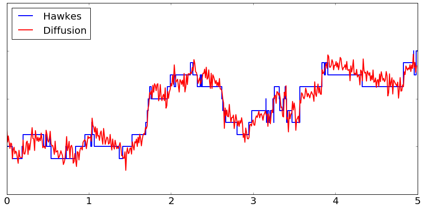
In Empirical studies, the data is reformulated to apply the diffusion model because the original data is based on a tick structure. The large interval, i.e., , is set to one minute where a sufficiently large number of events are observed for the approximation. Figure 7 presents the procedure, with every one minute, the observed price is the base point to construct a diffusion process, which lies behind the tick structure. Within the interval, the paths of the discretized version of the diffusion model are simulated with 60 subintervals.
4 Empirical study
4.1 Data
For empirical studies, ultra high-frequency data of 10 stocks in the S&P 500 are used. As raw data in the first place, we reorganize the data in the following way:
- •
The historical data consists of the best bid, ask quotes of the stocks, and their dynamics over trading time with various exchanges.
- •
The mid-price dynamics of the best bid and ask quotes of each stock reported in the New York Stock Exchange (NYSE) from 10:00 to 15:30 are selected to avoid the seasonal effects observed in early or late in the market.
- •
In the original raw data, the time stamps have 1 second resolutions. If the prices changes are reported several times for one second, the price changes with equidistant intervals are redistributed over one second.
- •
The mid-price increments and decrements have a unit size of change that is the half of the minimal bid ask spread. If a price increment or decrement is larger than the minimal unit size, the change is considered to be the sum of the successive movements with the minimal size. In recent data, the percentage of the minimal change is very high in many symbols, as listed in Table 2. In addition, Table 3 lists the percentage of minimal change of transacted prices where similar patterns to the percentage of the mid-prices are observed.
- •
The symbols in the table represents:
BAC - Bank of America Corp, CVX - Chevron, GE - General Electric Co., IBM - International Business Machines, JPM - JP Morgan Chase & Co, KO - The Coca-Cola Company, MCD - McDonald’s Corp, T - AT&T Inc, VZ - Verizon Communications Inc, XOM - Exxon Mobil Corp
| BAC | CVX | GE | IBM | JPM | KO | MCD | T | VZ | XOM | |
|---|---|---|---|---|---|---|---|---|---|---|
| 2007 | 79.91 | 61.88 | 83.29 | 55.70 | 78.16 | 75.41 | 73.71 | 79.15 | 84.57 | 70.14 |
| 2008 | 87.83 | 59.01 | 79.93 | 43.65 | 59.68 | 67.48 | 58.07 | 68.58 | 69.48 | 68.57 |
| 2009 | 88.19 | 70.36 | 93.84 | 56.98 | 72.42 | 80.10 | 84.51 | 82.14 | 82.06 | 86.79 |
| 2010 | 79.78 | 87.83 | 98.74 | 77.48 | 95.77 | 94.61 | 83.88 | 82.40 | 82.71 | 86.98 |
| 2011 | 99.53 | 72.16 | 99.21 | 52.73 | 96.96 | 89.44 | 86.92 | 98.23 | 89.07 | 90.35 |
| BAC | CVX | GE | IBM | JPM | KO | MCD | T | VZ | XOM | |
|---|---|---|---|---|---|---|---|---|---|---|
| 2007 | 92.70 | 69.86 | 97.26 | 64.40 | 90.34 | 89.81 | 87.23 | 94.74 | 93.11 | 79.78 |
| 2008 | 84.60 | 50.88 | 89.81 | 51.80 | 71.21 | 76.61 | 63.89 | 86.87 | 82.79 | 60.93 |
| 2009 | 98.89 | 72.34 | 98.39 | 59.98 | 88.03 | 89.15 | 80.42 | 97.44 | 93.67 | 82.47 |
| 2010 | 99.63 | 81.07 | 99.61 | 80.88 | 95.58 | 92.59 | 85.65 | 99.15 | 98.19 | 92.36 |
| 2011 | 99.81 | 62.08 | 99.68 | 57.04 | 96.76 | 91.76 | 80.58 | 99.01 | 97.12 | 84.48 |
4.2 Dynamics of parameters and performance of volatility measure
The parameters of the symmetric Hawkes process were estimated, as explained in C using the mid-price dynamics of the stocks quoted in NYSE. The estimations are employed on a daily basis because there are enough samples even in a day and the aim is to demonstrate the daily change in the parameters. Table 4 lists one of the results with GE for each day from January 3 to 27, 2011. The estimates of and their numerically computed standard errors in the parentheses are reported. In the estimation, the unit time, , is one second. The averaged daily estimates of for the different stocks over a month, January 2011, are also reported.
| Date | H.vol | TSRV | RRV | ||||
|---|---|---|---|---|---|---|---|
| 0103 | 0.0067 | 0.4661 | 1.3576 | 2.2596 | 0.0957 | 0.1289 | 0.1103 |
| (0.0004) | (0.0609) | (0.0958) | (0.1160) | ||||
| 0104 | 0.0082 | 0.4853 | 1.3941 | 2.5297 | 0.1139 | 0.1468 | 0.1344 |
| (0.0005) | (0.0494) | (0.0889) | (0.1104) | ||||
| 0105 | 0.0112 | 0.4741 | 1.1698 | 2.2281 | 0.1339 | 0.1825 | 0.1619 |
| (0.0006) | (0.0402) | (0.0673) | (0.0939) | ||||
| 0106 | 0.0091 | 0.5599 | 1.0112 | 2.1822 | 0.1265 | 0.1656 | 0.1391 |
| (0.0005) | (0.0471) | (0.0675) | (0.0958) | ||||
| 0107 | 0.0163 | 0.6973 | 0.5968 | 1.9959 | 0.1933 | 0.1998 | 0.1932 |
| (0.0007) | (0.0407) | (0.0391) | (0.0747) | ||||
| 0110 | 0.0132 | 0.4978 | 0.7434 | 1.8366 | 0.1520 | 0.1730 | 0.1553 |
| (0.0006) | (0.0360) | (0.0465) | (0.0780) | ||||
| 0111 | 0.0081 | 0.6959 | 0.7522 | 2.1448 | 0.1310 | 0.1414 | 0.1254 |
| (0.0005) | (0.0593) | (0.0645) | (0.1125) | ||||
| 0112 | 0.0098 | 0.4210 | 0.7322 | 1.8399 | 0.1181 | 0.1440 | 0.1328 |
| (0.0005) | (0.0406) | (0.0559) | (0.0965) | ||||
| 0113 | 0.0097 | 0.6512 | 0.3476 | 1.7471 | 0.1533 | 0.1275 | 0.1434 |
| (0.0005) | (0.0526) | (0.0379) | (0.1035) | ||||
| 0114 | 0.0092 | 0.6173 | 0.5303 | 1.8327 | 0.1390 | 0.1328 | 0.1344 |
| (0.0005) | (0.0533) | (0.0498) | (0.1097) | ||||
| 0118 | 0.0097 | 0.5122 | 0.4779 | 1.6361 | 0.1351 | 0.1235 | 0.1161 |
| (0.0005) | (0.0449 | (0.0434) | (0.0976) | ||||
| 0119 | 0.0168 | 0.4737 | 0.5202 | 1.5618 | 0.1774 | 0.1842 | 0.1772 |
| (0.0007) | (0.0331) | (0.0351) | (0.0772) | ||||
| 0120 | 0.0181 | 0.6944 | 0.5065 | 1.9431 | 0.2071 | 0.1913 | 0.1928 |
| (0.0007) | (0.0428) | (0.0359) | (0.0835) | ||||
| 0121 | 0.0316 | 0.5334 | 0.5986 | 1.7352 | 0.2358 | 0.2168 | 0.2299 |
| (0.0010) | (0.0262) | (0.0282) | (0.0556) | ||||
| 0124 | 0.0120 | 0.4355 | 0.4512 | 1.4181 | 0.1408 | 0.1249 | 0.1388 |
| (0.0006) | (0.0352) | (0.0358) | (0.0836) | ||||
| 0125 | 0.0209 | 0.6164 | 0.4259 | 1.6312 | 0.2144 | 0.2018 | 0.2096 |
| (0.0008) | (0.0321) | (0.0275) | (0.0640) | ||||
| 0126 | 0.0143 | 0.5053 | 0.5590 | 1.6587 | 0.1532 | 0.1146 | 0.1326 |
| (0.0007) | (0.0365) | (0.0390) | (0.0815) | ||||
| 0127 | 0.0147 | 0.5029 | 0.3925 | 1.4351 | 0.1687 | 0.1807 | 0.1578 |
| (0.0007) | (0.0371) | (0.0317) | (0.0868) |
| Symbol | ||||
|---|---|---|---|---|
| GE | 0.0141 | 0.5480 | 0.6766 | 1.8476 |
| IBM | 0.1489 | 1.0057 | 0.5037 | 2.0986 |
| JPM | 0.0672 | 0.6330 | 0.4767 | 1.5806 |
| KO | 0.0357 | 0.6669 | 0.3153 | 1.4814 |
| MCD | 0.0478 | 0.7201 | 0.4177 | 1.6641 |
| T | 0.0153 | 0.4593 | 0.5157 | 1.4506 |
| VZ | 0.0216 | 0.7887 | 0.4669 | 1.8206 |
| XOM | 0.0691 | 0.5280 | 0.3482 | 1.2808 |
In the column, ‘H.vol’, the annualized daily volatility estimates computed by the estimates of the Hawkes parameters and using the formula in Proposition 3 are presented. In the column, ‘TSRV’, the two scaled realized volatilities introduced by Zhang et al., 2005 are compared and in the column, ‘RRV’, the volatility estimates proposed by Robert and Rosenbaum, 2011 based on the uncertainty zones model are presented. The table shows that the Hawkes volatility, TSRV and RRV have similar values all over the reported time.
Figure 8 plots the dynamics of the parameters of GE, 2011. The estimation results show evidence that the parameters of the Hawkes process, particularly , changes with time. The dynamics of with time shows the typical movements of positively autocorrelated time series, which is strongly associated with the macro feature of the volatility movement, such as the GARCH effect and stochastic volatility. In addition, a comparison of Figures 8(a), 8(b) and 8(c) verifies that the dynamics of is related significantly to the dynamics of the volatility. When the parameter of a day is large, the volatility of the day is large and when the parameter of a day is small, the volatility of the day is small.
In the figure, the movements of the other parameters and , do not appear to be meaningful compared to the movement of . The plots also show that the volatilities computed by the symmetric Hawkes modeling and TSRV show similar patterns over the observed time period.
Figure 9 presents the parameter and volatility dynamics of GE, 2010. Similar to the previous case, the behaviors and TSRV are similar. The day of peaked volatilities in the figure is the May 6, 2010 Flash Crash where the equity prices fell rapidly. At the day of the Flash Crash, the two estimated volatilities had different values and TSRV was much larger than the Hawkes volatility.
In addition, in Figure 10, the estimated Hawkes volatility, TSRV and RRV of T (left) and MCD (right) are compared. All three volatilities have similar forms of movements during the observed period. For T, the Hawkes volatility was close to TSRV (right) at the day of Flash Crash. The estimated Hawkes volatility of MCD at the Flash Crash was larger than the TSRV or RRV.
Figure 11 plots the dynamics of the estimated parameters of GE in 2008, the starting year of the global financial crisis. The dramatic changes in the Hawkes volatility, TSRV, and were observed in the beginning of the crisis around August 2008. The mutual excited parameter, , was rather stable.
The volatility estimation results were compared using the Hawkes model and TSRV method in Table 6 with 10 symbols from 2007 to 2011. In each panel of the table, the mean of the Hawkes volatility and TSRV for given year and mean percentage error are presented. The volatility estimated by the symmetric Hawkes model is generally larger than the TSRV and the differences between the two volatilities are around 15-25%. The reason for the discrepancy between the TSRV and the Hawkes volatility is unknown. Possible reasons include the intraday variation of the parameters as in the Flash Crash and the restrictions in the parameter condition for the symmetry. These two issues are examined in the following subsections.
| BAC | CVX | GE | IBM | JPM | KO | MCD | T | VZ | XOM | |
|---|---|---|---|---|---|---|---|---|---|---|
| 2007 | ||||||||||
| H.vol | 0.1725 | 0.2387 | 0.1406 | 0.1674 | 0.2170 | 0.1290 | 0.1494 | 0.1731 | 0.1615 | 0.2327 |
| TSRV | 0.1555 | 0.1834 | 0.1323 | 0.1380 | 0.1899 | 0.1118 | 0.1296 | 0.1615 | 0.1433 | 0.1730 |
| MPE(%) | 14.93 | 20.28 | 12.34 | 17.26 | 15.91 | 15.58 | 15.87 | 14.04 | 14.26 | 23.14 |
| 2008 | ||||||||||
| H.vol | 0.7008 | 0.5129 | 0.3646 | 0.3939 | 0.6929 | 0.2583 | 0.3286 | 0.3751 | 0.3806 | 0.4592 |
| TSRV | 0.4880 | 0.3077 | 0.3172 | 0.2658 | 0.4868 | 0.2031 | 0.2440 | 0.3069 | 0.2930 | 0.2827 |
| MPE(%) | 28.14 | 33.17 | 13.57 | 28.41 | 26.61 | 19.60 | 21.34 | 16.09 | 19.97 | 32.53 |
| 2009 | ||||||||||
| H.vol | 0.7397 | 0.2608 | 0.3439 | 0.2166 | 0.4701 | 0.1762 | 0.1883 | 0.2407 | 0.2029 | 0.2198 |
| TSRV | 0.5420 | 0.2029 | 0.3367 | 0.1664 | 0.3722 | 0.1509 | 0.1607 | 0.1934 | 0.1810 | 0.1773 |
| MPE(%) | 25.42 | 21.48 | 9.12 | 20.81 | 17.97 | 15.23 | 15.79 | 20.27 | 13.43 | 18.26 |
| 2010 | ||||||||||
| H.vol | 0.2869 | 0.1758 | 0.1963 | 0.1395 | 0.2223 | 0.1138 | 0.1258 | 0.1461 | 0.1578 | 0.1603 |
| TSRV | 0.2234 | 0.1376 | 0.1952 | 0.1184 | 0.1985 | 0.1031 | 0.1040 | 0.1255 | 0.1241 | 0.1291 |
| MPE(%) | 21.20 | 21.11 | 11.47 | 17.07 | 13.46 | 13.51 | 18.12 | 15.96 | 17.73 | 18.86 |
| 2011 | ||||||||||
| H.vol | 0.3426 | 0.2197 | 0.2389 | 0.1681 | 0.2554 | 0.1334 | 0.1297 | 0.1460 | 0.1543 | 0.1872 |
| TSRV | 0.2648 | 0.1719 | 0.1921 | 0.1334 | 0.2146 | 0.1091 | 0.1122 | 0.1227 | 0.1228 | 0.1553 |
| MPE(%) | 13.79 | 20.46 | 18.78 | 18.49 | 17.06 | 19.24 | 15.73 | 17.47 | 20.38 | 17.38 |
4.3 Intraday volatility
One of the interesting applications to modeling the daily price dynamics using the symmetric Hawkes process is that the intraday volatility can be estimated in almost every moment of the day. This is possible because every arrival time of price change, which are plentiful even during ten minutes, is used and the maximum likelihood estimation is so powerful that the parameters can be estimated with similar or less than ten minutes data. Figure 12 shows the dynamics of the intraday volatility of GE with randomly chosen days. The first estimation of each day was performed using the first ten minutes data of each day. In this example, it ranged from 10:00 a.m. to 10:10 a.m.
The price movement histories were then updated in every ten minutes and the intraday volatilities were re-estimated using the updated data and already existing one. For the estimation, the reparametrization in Remark 2 were used and hence the annualized volatility was estimated directly by the maximum likelihood estimation with its numerically computed standard error. The solid lines in the figure represent the annualized volatilities estimated by the intraday data up to the time and the dotted lines represent the standard errors. In Figures 12(a) and 12(b), the volatilities are generally large at the beginning of the day and tend to decreases, which is consistent with the seasonality effect in that in the early markets, more trading activities are observed than the middle of the day.
Figure 12(c) shows the data for the 2010/05/06 Flash Crash and a dramatic increase was observed in the late part of the day. Similar behavior is presented in Figure 12(d), which is for the intraday volatility of VZ in the 2010/05/06 Flash Crash. The real time volatility measurement technique will be very useful in intraday risk managements, because investors can respond to sudden market changes more effectively, if they can compute the exact volatility variation.
4.4 Fully characterized Hawkes process
The maximum likelihood estimation of the Hawkes process with full characterization of the parameters as explained in Subsection 2.2 was performed. As in the previous subsection, the estimations were employed on a daily basis. In Figure 13, the dynamics of all parameters of the fully characterized Hawkes model of GE in 2011 are plotted.
The dynamics of the parameters are close to each other in the mean, as illustrated in Figure 13(a) which suggest that in the long run sense. Similarly, each pair of parameters of , , , and are close to each other in the mean. The dynamics of the parameters and fluctuate more than and over time. The sample means of and of GE in 2011 are quite close to and as reported in panel A of Table 7. The row ‘std.’ in the table is the sample standard deviation of the time series of each parameter over the time period.
On the other hand, the parameters are not always close to among others in the mean. In the panel B of the table which presents the estimates of the parameters of XOM in 2008, the estimates of and are close to each other and similarly, the estimates of and are close to each other in the mean, but the estimates of and are significantly different in the mean. Similarly, the difference in the estimates of and are significant. In this case, the self-excited effects are less persistent than the mutually excited effects.
| A | ||||||||||
| mean | 0.0198 | 0.0199 | 0.5196 | 0.5228 | 0.3235 | 0.3165 | 1.4145 | 1.4128 | 1.5574 | 1.5378 |
| std. | 0.0124 | 0.0128 | 0.1108 | 0.1241 | 0.1902 | 0.1875 | 0.2097 | 0.2463 | 0.5856 | 0.5402 |
| B | ||||||||||
| mean | 0.1886 | 0.1727 | 1.0594 | 0.9904 | 0.1369 | 0.1288 | 1.7648 | 1.6916 | 0.8972 | 0.7329 |
| std. | 0.1187 | 0.1196 | 0.3274 | 0.3348 | 0.0850 | 0.0786 | 0.4478 | 0.4480 | 0.6104 | 0.5197 |
4.5 Diffusion parameter
The parameters of the diffusion model introduced in subsection 3.1 were estimated using the simulated likelihood estimation explained in subsection 3.4. The results of GE, January 2011 are presented in Table 8 and are similar to the results with the Hawkes model in Table 4. In addition, the estimates of the diffusion model with are presented in Table 9. The estimates in each model show the similar patterns over the period.
The diffusion estimation has its own pros and cons. In our setting, because the observed values of the price over one minute intervals are only used, which is in contrast to the Hawkes modeling where all times of price changes are used, the diffusion estimator is less efficient than the Hawkes estimator. In addition, by the nature of the simulated likelihood estimation, it takes longer time to compute the likelihoods and the computed results are not deterministic but depend on the random numbers generated by computers. On the other hand, when the observing times of a price process are limited, i.e., the prices are only available at each one minute interval, the diffusion model and its estimation are a feasible alternate choice to examine the nature of the price movements in high-frequency.
| Date | volatility | ||||
|---|---|---|---|---|---|
| 0103 | 0.0137 | 0.1225 | 1.9872 | 2.5512 | 0.1392 |
| 0104 | 0.0091 | 0.0805 | 2.9568 | 3.3122 | 0.1546 |
| 0105 | 0.0089 | 0.7037 | 2.7975 | 3.5694 | 0.3661 |
| 0106 | 0.0082 | 1.0110 | 2.1844 | 3.3689 | 0.2511 |
| 0107 | 0.0196 | 0.8574 | 1.3001 | 2.5649 | 0.2557 |
| 0110 | 0.0140 | 0.7615 | 0.7941 | 2.3103 | 0.1739 |
| 0111 | 0.0069 | 0.5888 | 2.1067 | 2.9101 | 0.1710 |
| 0112 | 0.0046 | 0.3888 | 1.5751 | 2.4639 | 0.1247 |
| 0113 | 0.0105 | 0.6536 | 0.7633 | 2.3407 | 0.1314 |
| 0114 | 0.0043 | 0.9421 | 1.2195 | 2.2284 | 0.2833 |
| 0118 | 0.0093 | 0.7737 | 0.7164 | 1.7152 | 0.2325 |
| 0119 | 0.0174 | 0.5661 | 1.1345 | 2.3551 | 0.1714 |
| 0120 | 0.0173 | 0.7892 | 1.0437 | 2.6670 | 0.1844 |
| 0121 | 0.0342 | 0.5358 | 1.1074 | 2.3377 | 0.2215 |
| 0124 | 0.0142 | 0.4669 | 0.8490 | 2.0244 | 0.1349 |
| 0125 | 0.0208 | 0.7222 | 0.9767 | 2.1042 | 0.2308 |
| 0126 | 0.0135 | 0.6058 | 1.0571 | 2.4183 | 0.1387 |
| 0127 | 0.0157 | 0.6458 | 0.8145 | 1.8174 | 0.2043 |
| Date | |||||
|---|---|---|---|---|---|
| 0103 | 0.0140 | 0.0191 | 1.9107 | 2.4863 | 0.2010 |
| 0104 | 0.0094 | 0.4947 | 2.3869 | 3.2896 | 0.1106 |
| 0105 | 0.0083 | 0.4363 | 3.0567 | 3.5328 | -0.0338 |
| 0106 | 0.0097 | 0.7811 | 2.3254 | 3.4391 | -0.0952 |
| 0107 | 0.0196 | 0.8110 | 1.5196 | 2.6318 | -0.3633 |
| 0110 | 0.0067 | 0.5657 | 1.7872 | 2.3712 | 0.0397 |
| 0111 | 0.0072 | 0.7457 | 1.7410 | 2.5917 | 0.0229 |
| 0112 | 0.0116 | 0.4343 | 1.4936 | 2.7054 | -0.1048 |
| 0113 | 0.0114 | 0.7440 | 0.8413 | 2.2652 | -0.0709 |
| 0114 | 0.0051 | 0.8205 | 1.2866 | 2.1705 | -0.0087 |
| 0118 | 0.0045 | 0.1585 | 1.6107 | 1.7917 | 0.1269 |
| 0119 | 0.0185 | 0.4916 | 1.1835 | 2.3827 | -0.2130 |
| 0120 | 0.0153 | 0.5343 | 0.9029 | 1.9994 | 0.1086 |
| 0121 | 0.0164 | 0.6817 | 1.1065 | 1.9896 | -0.1220 |
| 0124 | 0.0148 | 0.5293 | 1.0546 | 1.9986 | -0.0055 |
| 0125 | 0.0252 | 0.6536 | 0.9445 | 2.0343 | 0.1237 |
| 0126 | 0.0156 | 0.5248 | 1.0506 | 2.3678 | 0.0473 |
| 0127 | 0.0167 | 0.5304 | 0.8537 | 1.6645 | 0.0800 |
5 Conclusion
This paper examined the empirical performance of the symmetric Hawkes process which is a simple model to consider for both clustering property and market microstructure noise in volatility estimation using the stock prices in the S&P 500. The daily dynamics of the Hawkes parameters, the comparison between the Hawkes volatility and the realized volatility and the intraday volatility estimation procedure are discussed. The diffusion analogy of the symmetric Hawkes model was also proposed to provide the analytical simplicity for computing the distributional properties. The diffusion model also incorporates the clustering effect, market microstrucutre noise, in addition to asymmetric property.
The volatility could be estimated over a relatively short time interval with the Hawkes model and the intraday variations of volatility was demonstrated. A comparison between the Hawkes volatility and TSRV showed the difference around 15-25%. The parameter restriction, asymmetry and parameter variations might be the cause of the discrepancy but more work will be needed to understand the exact reason. The estimation results of the diffusion model were provided where similar patterns to the Hawkes model parameters were observed.
References
- Aït-Sahalia et al., (2010) Aït-Sahalia, Y., Cacho-Diaz, J., and Laeven, R. J. (2010). Modeling financial contagion using mutually exciting jump processes. Technical report, National Bureau of Economic Research.
- Aït-Sahalia et al., (2008) Aït-Sahalia, Y. et al. (2008). Closed-form likelihood expansions for multivariate diffusions. The Annals of Statistics, 36(2):906–937.
- Ait-Sahalia et al., (2013) Ait-Sahalia, Y., Fan, J., and Li, Y. (2013). The leverage effect puzzle: Disentangling sources of bias at high frequency. Journal of Financial Economics, 109:224–249.
- Aït-Sahalia et al., (2005) Aït-Sahalia, Y., Mykland, P. A., and Zhang, L. (2005). How often to sample a continuous-time process in the presence of market microstructure noise. Review of Financial studies, 18:351–416.
- Aït-Sahalia et al., (2011) Aït-Sahalia, Y., Mykland, P. A., and Zhang, L. (2011). Ultra high frequency volatility estimation with dependent microstructure noise. Journal of Econometrics, 160:160–175.
- Andersen et al., (2003) Andersen, T. G., Bollerslev, T., Diebold, F. X., and Labys, P. (2003). Modeling and forecasting realized volatility. Econometrica, 71:579–625.
- Bacry et al., (2012) Bacry, E., Dayri, K., and Muzy, J.-F. (2012). Non-parametric kernel estimation for symmetric Hawkes processes. application to high frequency financial data. The European Physical Journal B-Condensed Matter and Complex Systems, 85:1–12.
- Bacry et al., (2013) Bacry, E., Delattre, S., Hoffmann, M., and Muzy, J.-F. (2013). Modelling microstructure noise with mutually exciting point processes. Quantitative Finance, 13:65–77.
- Bacry and Muzy, (2014) Bacry, E. and Muzy, J.-F. (2014). Hawkes model for price and trades high-frequency dynamics. Quantitative Finance, 14:1147–1166.
- (10) Barndorff-Nielsen, O. E. and Shephard, N. (2002a). Econometric analysis of realized volatility and its use in estimating stochastic volatility models. Journal of the Royal Statistical Society: Series B (Statistical Methodology), 64:253–280.
- (11) Barndorff-Nielsen, O. E. and Shephard, N. (2002b). Estimating quadratic variation using realized variance. Journal of Applied Econometrics, 17:457–477.
- Bauwens and Hautsch, (2009) Bauwens, L. and Hautsch, N. (2009). Modelling financial high frequency data using point processes. In Handbook of Financial Time Series, pages 953–979. Springer Berlin Heidelberg.
- Bollerslev et al., (2011) Bollerslev, T., Gibson, M., and Zhou, H. (2011). Dynamic estimation of volatility risk premia and investor risk aversion from option-implied and realized volatilities. Journal of econometrics, 160(1):235–245.
- Bowsher, (2007) Bowsher, C. G. (2007). Modelling security market events in continuous time: Intensity based, multivariate point process models. Journal of Econometrics, 141:876–912.
- Brandt and Santa-Clara, (2002) Brandt, M. W. and Santa-Clara, P. (2002). Simulated likelihood estimation of diffusions with an application to exchange rate dynamics in incomplete markets. Journal of financial economics, 63:161–210.
- Brémaud, (1981) Brémaud, P. (1981). Point Processes and Queues : Martingale Dynamics. Springer.
- Broyden, (1970) Broyden, C. G. (1970). The convergence of a class of double-rank minimization algorithms 1. general considerations. IMA Journal of Applied Mathematics, 6:76–90.
- (18) Choe, G. H. and Lee, K. (2014a). Conditional correlation in asset return and garch intensity model. AStA Advances in Statistical Analysis, 98:197–224.
- (19) Choe, G. H. and Lee, K. (2014b). High moment variations and their application. Journal of Futures Markets, 34:1040–1061.
- (20) Da Fonseca, J. and Zaatour, R. (2014a). Clustering and mean reversion in a Hawkes microstructure model. Journal of Futures Markets, 35:813–838.
- (21) Da Fonseca, J. and Zaatour, R. (2014b). Hawkes process: Fast calibration, application to trade clustering, and diffusive limit. Journal of Futures Markets, 34:548–579.
- Daley and Vere-Jones, (2003) Daley, D. J. and Vere-Jones, D. (2003). An introduction to the theory of point processes, volume 1. Springer.
- Dassios and Zhao, (2012) Dassios, A. and Zhao, H. (2012). Ruin by dynamic contagion claims. Insurance: Mathematics and Economics, 51:93–106.
- El Euch et al., (2016) El Euch, O., Masaaki, F., and Mathieu, R. (2016). The microstructural foundations of leverage effect and rough volatility. arXiv preprint arXiv:1609.05177.
- Embrechts et al., (2011) Embrechts, P., Liniger, T., Lin, L., et al. (2011). Multivariate hawkes processes: an application to financial data. Journal of Applied Probability, 48:367–378.
- Errais et al., (2010) Errais, E., Giesecke, K., and Goldberg, L. R. (2010). Affine point processes and portfolio credit risk. SIAM Journal on Financial Mathematics, 1:642–665.
- Garcia et al., (2011) Garcia, R., Lewis, M.-A., Pastorello, S., and Renault, É. (2011). Estimation of objective and risk-neutral distributions based on moments of integrated volatility. Journal of Econometrics, 160(1):22–32.
- Hansen and Lunde, (2006) Hansen, P. R. and Lunde, A. (2006). Realized variance and market microstructure noise. Journal of Business and Economic Statistics, 24:127–161.
- (29) Hawkes, A. G. (1971a). Point spectra of some mutually exciting point processes. Journal of the Royal Statistical Society. Series B (Methodological), pages 438–443.
- (30) Hawkes, A. G. (1971b). Spectra of some self-exciting and mutually exciting point processes. Biometrika, 58:83–90.
- Hawkes and Oakes, (1974) Hawkes, A. G. and Oakes, D. (1974). A cluster process representation of a self-exciting process. Journal of Applied Probability, pages 493–503.
- Henningsen and Toomet, (2011) Henningsen, A. and Toomet, O. (2011). maxlik: A package for maximum likelihood estimation in R. Computational Statistics, 26:443–458.
- Heston, (1993) Heston, S. (1993). A closed-form solution for options with stochastic volatility with applications to bond and currency options. Review of Financial Studies, 6:327–343.
- Hewlett, (2006) Hewlett, P. (2006). Clustering of order arrivals, price impact and trade path optimisation. In Workshop on Financial Modeling with Jump processes, Ecole Polytechnique.
- Jaisson et al., (2015) Jaisson, T., Rosenbaum, M., et al. (2015). Limit theorems for nearly unstable Hawkes processes. The Annals of Applied Probability, 25:600–631.
- Large, (2007) Large, J. (2007). Measuring the resiliency of an electronic limit order book. Journal of Financial Markets, 10:1–25.
- Lee, (2016) Lee, K. (2016). Probabilistic and statistical properties of moment variations and their use in inference and estimation based on high frequency return data. Studies in Nonlinear Dynamics & Econometrics, 20:19–36.
- Li and Fukushima, (2001) Li, D.-H. and Fukushima, M. (2001). On the global convergence of the bfgs method for nonconvex unconstrained optimization problems. SIAM Journal on Optimization, 11:1054–1064.
- Nash et al., (2014) Nash, J. C. et al. (2014). On best practice optimization methods in R. Journal of Statistical Software, 60.
- Ogata, (1978) Ogata, Y. (1978). The asymptotic behaviour of maximum likelihood estimators for stationary point processes. Annals of the Institute of Statistical Mathematics, 30:243–261.
- Robert and Rosenbaum, (2011) Robert, C. Y. and Rosenbaum, M. (2011). A new approach for the dynamics of ultra-high-frequency data: The model with uncertainty zones. Journal of Financial Econometrics, 9:344–366.
- Zhang et al., (2005) Zhang, L., Mykland, P. A., and Aït-Sahalia, Y. (2005). A tale of two time scales. Journal of the American Statistical Association, 100:1394–1411.
- Zheng et al., (2014) Zheng, B., Roueff, F., and Abergel, F. (2014). Modelling bid and ask prices using constrained Hawkes processes: Ergodicity and scaling limit. SIAM Journal on Financial Mathematics, 5:99–136.
Appendix A Expected intensity of fully characterized Hawkes model
Consider the conditional expectation of the intensity processes:
Then, for each ,
and by differentiating both sides with respect to ,
In addition, with the similar method, for ,
The differential equation system is represented by the matrix form
When the eigenvalues of the matrix are negative, the particular solution of the system becomes the long-run expectations of the intensities and are given by
as , where
The above formulas can be used as the presumed initial values of the intensity processes in the simulations or estimation procedures. With full characterization of the parameters , the system is four dimensional and the solution is rather complicated.
Appendix B Simulation method
If the decaying parameters are different from each other, the system of the self and mutually excited Hawkes and intensity processes are not Markov. As shown in Eq. (1), depends on both and , for , and similarly, depends on both and . On the other hand, the whole system of the processes are Markov and to generate the future paths, it is only important to know the current values of not the entire past histories of the processes. Therefore, for the simulation of the Hawkes process, it is important to compute the distributions of the arrival times determined by each component of the intensities, and .
Suppose that, over a time interval , there is no jump by and ; then the intensities are deterministic and exponentially decaying function is
Note that can be represented by the sum of three jump components , and independent upon with the corresponding intensities , , and , respectively. Let be the first interarrival time of with intensity after . The probability distribution of is then represented by
Thus,
where is a uniformly distributed random variable over [0,1]. In addition, let denote a random variable that follows a Poisson distribution with intensity . Then becomes the next jump arrival time after . After a jump occur, the counting processes are updated accordingly, the intensities are updated, as in Eqs. (1) and (2), and the above procedure is applied repeatedly.
Appendix C Likelihood function
Let be the -th jump arrival time of and be the interarrival time between and -th jumps. Then the conditional cumulative distributions of at time , i.e., with given , is
Therefore, the conditional density functions is
Similarly, let be the -th jump arrival time of and be the interarrival time between the and -th jumps. The conditional density function of at time is then
Now consider the interval over which the jumps are observed. The log-likelihood of the realized jump arrivals up to time is represented by the sum of log-likelihood of all realized arrivals of and . That is
where denotes the parameter vector. The maximum likelihood estimator, , is the estimator which maximize under the observations of realized jump arrivals of and .
Define a matrix with each element
The maximum likelihood estimator converges to the true parameter value asymptotically normally in distribution with an asymptotic variance-covariance matrix , see Ogata, 1978. For the maximum likelihood estimation in the statistical package R, consult Henningsen and Toomet, 2011.
Appendix D Proof of the variance formula in Proposition 3
In this section, the variance formula is derived under the symmetric Hawkes process assumption of the price process. When the price follows Eq. (4) with symmetric Hawkes process, the variance of the return is represented by
To compute the variance of the return over time interval , the following results are needed. The intensities and are assumed to be in the stationary state at time . Under the assumption, the variance of the price process is derived using the stochastic integration theory. The quadratic variation of is defined by
and the quadratic covariation of and is defined as
When the processes are quadratic pure jump processes, i.e., the quadratic (co)variation of the continuous part is zero,
Without a loss of generality, it is assumed that in this proof. The next lemma is stated without proof.
Lemma 6.
Under the stationarity condition of the intensities at time 0,
Recall that
Lemma 7.
Under the stationarity condition of the intensities at time 0,
for some constant and .
Proof.
Note that
and
Therefore, a system of equations can be derived:
The particular solution of the system is
where the inverse matrix of is represented by
In addition, the general solution is
and with the initial condition of (8),
∎
Lemma 8.
Under the stationary state condition of the intensities at time 0, we have
Proof.
Note that
and
In the above, is replaced with due to the symmetry of the model and similarly, is replaced with . Therefore, following system of equations can be derived:
where the previous lemma is used. The particular solution is
where
and
and . The general solution is
and with the initial condition,
∎
Proposition 9.
Under the stationary state condition of the intensities at time 0,
In addition,
Proof.
The following is used:
and
along with the previous lemmas. In the above equation, as the probability of the simultaneous jumps of and is zero. In addition, under the symmetry. Therefore,
∎
Appendix E Proof of Proposition 4
Note that
Let
and
By assumming ,
Thus,
and
In addition,
Thus,
and
Therefore,
and the desired result is obtained.
Appendix F Proof of Proposition 5
As
and
we have
Note that
For the last equality, the following assumption is used:
The following can be derived:
Similarly
Let
and
and
Thus,
and
Therefore,
and hence
Finally,