Robust Translational Force Control of Multi-Rotor UAV for Precise Acceleration Tracking*

The first candidate is to time-synchronize the attitude and total thrust output by adding an artificial time delay to $T_{t,d}$ in Equation (9) as

Here, $\gamma_{v}$ is a delay element deliberately applied to $\tilde{\ddot{z}}_{d}$. Applying Equation (13) to Equation (11), the equation of motion is changed from Equation (12) to

Through Equations (7), (8) and (10), $\phi(t)$ and $\theta(t)$ can be described as

Let us assume that $\gamma_{\phi}$ and $\gamma_{\theta}$ have the same value of $\gamma_{h}$ since most multi-rotors have nearly the same roll and pitch behavior due to the symmetrical mechanical structure. Then, Equation (14) with Equations (10) and (15) becomes as

Now, we can solve the problem in Equation (12) by setting $\gamma_{v}$ equal to $\gamma_{h}$. However, this method is not easily applicable in a real-world situation because it is difficult to determine the value of $\gamma_{h}$ that changes continuously during the flight. Therefore, the control method through Equation (13) cannot be a practical method.

Alternatively, we can find a reasonable solution that is applicable in the real world by selectively delaying $\phi_{d}(t)$ and $\theta_{d}(t)$ in Equation (13) by $\gamma_{\phi}$ and $\gamma_{\theta}$, but keeping $\gamma_{v}$ at zero. As we can see from Equation (10), the values of $\phi_{d}(t)$ and $\theta_{d}(t)$ delayed by $\gamma_{\phi}$ and $\gamma_{\theta}$ seconds are $\phi(t)$ and $\theta(t)$. Applying this idea to Equation (13), we can obtain $T_{t,d}$ as

where the values $\phi(t)$ and $\theta(t)$ can be measured from the built-in inertial measurement unit (IMU) sensor. Then, by setting $\gamma_{v}$ to zero, we can determine the input/output relationship of the translational accelerations dynamics of the multi-rotor as

where we assume ${{\tilde{\ddot{z}}_{d}(t)}\over{\tilde{\ddot{z}}_{d}(t-\gamma_{h})}}\approx 1$. This assumption is valid in most cases, except in situations where the change in target vertical acceleration is abnormally large and rapid.

Through the control techniques of solution candidate 2 (Equations (7), (8) and (17)), we obtained a three-dimensional translational acceleration control method applicable to actual multi-rotor control. In order to compare the performance of multi-rotor control using Equations (9) and (17), a brief simulation is conducted as shown in Fig. 3.

The simulation shows the comparison of the target acceleration tracking performance of Case 1 with Equations (7), (8), (9) and Case 2 with Equations (7), (8), (17). The upper set of figures show the acceleration tracking performance of Cases 1 and 2 with arbitrary acceleration command. Here, we can see that there are no differences in performance between Cases 1 and 2 when MOI of the multi-rotor has small value of 0.1. On the other hand, when the MOI of the multi-rotor increases, both Cases 1 and 2 show delayed responses in the X and Y direction acceleration tracking as expected. However, we can observe that the Z-directional performance of the Case 2 remains the same regardless of the magnitude of the MOI, unlike Case 1 where the performance degradation is observed. The effect of the decline in Z-directional control performance on the system is evident when controlling the position of the multi-rotor. The bottom set of figures is the situation where the high-level position controller generates the desired acceleration command to track the predefined trajectory. In Case 1, we can observe a decrease in acceleration tracking performance in both the X and Y directions as well as the Z direction as the MOI increases. On the other hand, in Case 2, the Z-directional control performance remains constant regardless of the MOI of the platform, stabilizing the X and Y-directional control performance faster than Case 1.

This phenomenon can be understood in other ways by considering the role of the denominator term of the $T_{t}$ equation in Equation (6), which is to compensate for the reduction of the vertical thrust component in the sense of inertial coordinates when the multi-rotor is tilted. When $T_{t,d}$ is calculated based on the desired attitude as Equation (9), the situation is similar to compensating for the future event after $\gamma_{h}$ seconds. Instead, it is intuitive to use the current attitude as in Equation (17) to correct the vertical thrust reduction. From the flight results using Equation (17) in Fig. 3, we can confirm that the control performance in all directions is satisfactory.

For the estimation of $\mathbf{d}_{EID}$, we first estimate $\kappa$ the sum of $\tilde{\mathbf{F}}_{d}$ and $\mathbf{d}_{EID}$ by

We can easily achieve the $\tilde{\mathbf{F}}$ signal from Equation (19) where $\ddot{\mathbf{X}}$ is measured by the IMU sensor. The transfer function ${P_{n}(s)}$ is the nominal model of ${P(s)}$, and $\hat{(*)}$ is the representation of the estimation of $(*)$ signal throughout this paper. Once we estimate $\hat{\kappa}$, we then obtain $\hat{\mathbf{d}}_{EID}$ by

The signal $\hat{\kappa}(s)$ passes through the ${Q_{1}}$ block, which is basically a low pass filter, to overcome both the causality violation issue due to the improperness of ${P_{n}^{-1}}(s)$ and the potential instability issue caused by the non-minimum phase characteristic of ${P_{n}}(s)$. The filter ${Q_{2}}(s)$ is used to match the phase with ${Q_{1}}(s)\hat{\kappa}(s)$ signal. In the end, we generate a disturbance-compensating control input $\tilde{\mathbf{F}}_{d}$ by

This makes $\kappa$ become

The most important factor in the $\mathbf{d}_{EID}$ estimation process is the proper design of ${P_{n}}$ and ${Q}$. Of these, ${Q}$ is deeply related to the stability of the system and will be discussed in more detail in the next section. In the remainder of this section, we first discuss the design of the nominal model ${P_{n}}$ and then explain the structure of the $Q$-filter.

The internal structure of ${P_{n}^{-1}}(t)$ is described as in Fig. 5, all of which are simple conversion blocks except for the ${{\it{\Lambda}}}^{-1}_{n}{\it(t)}$ block. The block ${\it{\Lambda}}(t)$ is the relationship between $\mathbf{r}_{d}$ and $\mathbf{r}$ depicted in Fig. 2. The $\it{\Lambda_{n}(s)}$ is constructed from two parts: attitude and thrust dynamics. We denote these as $\it{\Lambda_{n,a}}(s)$ and $\it{\Lambda_{n,t}}(s)$ respectively.

As we see from Fig. 2, $\it{\Lambda}_{n,a}(s)$ is constructed with attitude controller, rotor dynamics and attitudinal dynamics. Since rotor dynamics can be ignored, we only need to find the transfer function of the attitudinal dynamics and attitude controller. For attitude dynamics, let us refer to Equation (2) and express it as

where $i=1,2,3$ represent $\phi$, $\theta$, $\psi$ axis, respectively. For attitude control, PD control in the following form is used.

The parameters $P_{i}$, $D_{i}$ represent control gains in each attitude component. Then, the overall transfer function ${\it{\Lambda}}_{n,a,i}$ between desired and current attitude becomes

In the case of ${\it{\Lambda}}_{n,t}$, the only dynamics involved is rotor dynamics, which we decided to neglect. Thus, it can be expressed as

Now, we can construct the transfer matrix for ${\it{\Lambda}}_{n}=diag({\it{\Lambda}}_{n,1},{\it{\Lambda}}_{n,2},{\it{\Lambda}}_{n,3})$ using Equations (26) and (27) as

Equation (28) is a detailed representation of the relationship between $\mathbf{r}_{d}$ and $\mathbf{r}$, which was introduced in Equation (10). On the other hand, $P_{n}$, which defines the nominal relationship between $\kappa$ and $\mathbf{F}$ (or $\tilde{\ddot{\mathbf{X}}}_{d}$ and $\tilde{\ddot{\mathbf{X}}}$), was introduced in Equation (18) (refer Equation (4) for the relationship between $\tilde{\ddot{\mathbf{X}}}$ and $\mathbf{F}$). Here, we can see that both Equations (10) and (18) have the same input/output characteristics with time delay of $\gamma_{h}$ for the first and second channels and no time delay for the third channel. Therefore, we can conclude that ${\it{\Lambda}}_{n}(s)$ in Equation (28) is also the transfer function between $\kappa$ and $\mathbf{F}$ as well as between $\mathbf{r}_{d}$ and $\mathbf{r}$, which is

In $Q$-filter design, we choose to make ${Q_{1}}(s){\it{\Lambda}}_{n}^{-1}(s)$, which is now identical to ${Q_{1}}(s){P}_{n}^{-1}(s)$, a proper function with relative degree of 1. Since ${P}_{n}(s)$ is composed of three channels in $X$, $Y$ and $Z$ directions, we need to design three separate $Q$-filters. As shown in Equation (26), ${\it{\Lambda}}_{n,1}(s)$($={\it{\Lambda}}_{n,a,2}(s)$) and ${\it{\Lambda}}_{n,2}(s)$($={\it{\Lambda}}_{n,a,1}(s)$) among the three transfer functions of ${\it{\Lambda}}_{n}(s)$ are systems with a relative degree of 1. The thrust transfer function ${\it{\Lambda}}_{n,3}(s)$($={\it{\Lambda}}_{n,t}(s)$) has a relative degree of 0, as can be seen from Equation (27). Therefore, the $Q$-filters for making ${Q_{1}}(s){\it{\Lambda}}_{n}^{-1}(s)$ with a relative degree of 1 are designed as

where ${Q_{1,h}}$ and ${Q_{1,v}}$ are $Q$-filters corresponding to the horizontal ($\it{\Lambda}_{n,a}$) and vertical ($\it{\Lambda}_{t}$) models respectively. The symbol $\tau$ is the time constant and $\zeta$ is the damping ratio of the filter. The filter ${Q_{1}}$ is designed to have a gain of 1 when $s=0$ [21]. The filter ${Q_{2}}$ is set to ${Q_{2}}={Q_{1}}$, to easily achieve the purpose of phase matching.

In [25], the structured singular value $\mu$ is defined as

where $\Delta$ is a complex structured block-diagonal unmodeled uncertainty block which gathers all model uncertainties [26]. Following the common notation, the symbol $\mathbf{\Delta}$ represents a set of all stable transfer matrices with the same structure (full, block-diagonal, or scalar blocks) and nature (real or complex) as $\Delta$. The $\bar{\sigma}\big(\Delta\big)$ is the maximum singular value of uncertainty block $\Delta$. The matrices $M$ and $\Delta$ are defined by collapsing the simplified overall system to upper LFT uncertainty description as

where $M$ is the known part of the system, $r$ is a reference input and $y$ is an output of the overall system. In the theory of the $\mu$-analysis, it is well-known that the system is robustly stable if $\mu$ satisfies the following conditions

[22][25].

The $\mu$-analysis is performed separately for each channel of $X$, $Y$, $Z$ thanks to the structure of the platform described by Equation (28), but since $X$ and $Y$ channels are composed of the same structure, they share the identical analysis result. As we can see from Fig. 7, the system is collapsed in the form of Equation (48) by using MATLAB’s Robust Control Toolbox${}^{\textrm{TM}}$, where $r_{j}=[\mathbf{F}_{d,j}\ \mathbf{d}_{EID,j}]^{T}\in\mathbb{R}^{2\times 1}$ and $y_{j}=\tilde{\mathbf{F}}_{j}\in\mathbb{R}$ in our case. As a reminder, subscript $j$ refers to each channel of $X$, $Y$, and $Z$. Also, structured uncertainty ${\Delta}_{j}(s)\in\mathbb{C}^{3\times 3}$ is constructed as

which includes unmodeled MOI uncertainty, time and gain uncertainty in our system.

Table I shows the multi-rotor’s physical quantities and controller gains used both in the simulation and the experiment. The gains $P_{\phi,\theta}$ and $D_{\phi,\theta}$ are predefined values set during the primary gain-tuning process to obtain the ability to control the attitude of the platform. The translational acceleration limit is set to prevent flight failure due to excessive acceleration control inputs and is set at $\pm 3\ $\mathrm{m}\mathrm{/}\mathrm{s}^{2}$$ to have a roll and pitch limit of approximately $\pm 0.3\ $\mathrm{r}\mathrm{a}\mathrm{d}$$ in level flight condition. As previously mentioned, the unmodeled time delay $\delta_{j}$ is set to 0.1, and the gain error is assumed to be a maximum error of 10 percent. For MOIs that are difficult to estimate, we assumed a wider 30 percent uncertainty. The damping ratio $\zeta$ of the second order filter is set to 0.707, which is the critical damping ratio, to balance the overshoot and late response. Fig. 8 shows the results of $\mu$-analysis. From the analysis, we can see that the system is stable when $\tau_{1}>0.12$ and $\tau_{2}>0.09$.

Fig. 9 shows the results of the SGT-based stability analysis, performed in the same manner as [18]. The analysis is based on the following model:

where all uncertainties due to $\delta_{j}$, $K_{j}$ and $J_{j}$ are lumped using the functions $W_{l,h}(=W_{l,1},W_{l,2})$ and $W_{l,v}(=W_{l,3})$, whose magnitude increases over frequency as shown in blue curves of Fig. 9. The stability condition of the SGT-based analysis in this case is

[18, 22, 27]. In the SGT-based analysis, the bode plots of the $Q$-filter with $\tau_{1}=0.12$ and $\tau_{2}=0.09$ indicate that system with those $\tau$ values could be unstable. However, through the $\mu$-analysis, those $\tau$ values are still in the stable region. From this, we can confirm that the $\mu$-analysis provides more rigorous $\tau$ boundary values than SGT-based analysis.

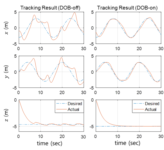
In the simulation, the multi-rotor follows a circular trajectory with radius of 3 $\mathrm{m}$ and height of 5 $\mathrm{m}$. Meanwhile, the multi-rotor is exposed to periodic disturbances with accelerations up to 5.5 $\mathrm{m}\mathrm{/}\mathrm{s}^{2}$ in each axis. Fig. 11 compares the multi-rotor’s position tracking performance before and after applying DOB. On the left graphs of Fig. 11, the target trajectory tracking results are not smooth due to the unexpected disturbances, whereas the trajectory deviation is drastically reduced in the right graphs where the DOB algorithm is applied.

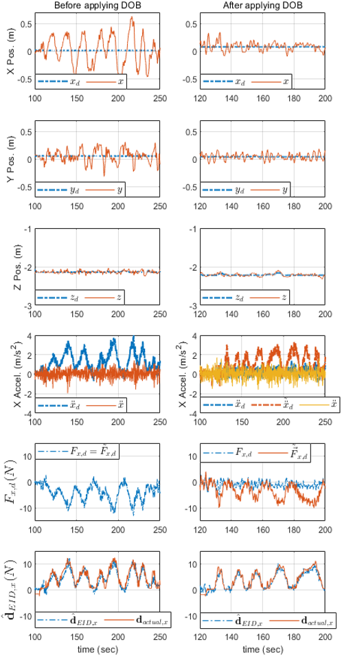
In the experiment, the multi-rotor is commanded to hover at a specific point in three-dimensional space but connected to the translational force measurement sensor via the tether to measure the applied disturbance force. As we can see in Fig. 13, the operator aligns the force sensor in the $X$-axis and pulls and releases the force sensor periodically to apply a disturbance to the multi-rotor.

Fig. 12 is a comparison of hovering performance before (left) and after (right) applying the DOB algorithm. The graphs in the left column are the case when the DOB is not applied, which has a larger $X$ directional position shift than other axes. Unlike the DOB-off case, the DOB-on case shows a significant reduction in position error.

Two graphs at the forth row shows the acceleration tracking results. When DOB is not applied, an acceleration signal is generated by the position error, but we can see that the target acceleration cannot be followed due to the disturbance. Meanwhile, we can see that the acceleration of the platform (yellow solid line) well tracks the target acceleration (blue dash-single dotted line). This is because the well-behaved DOB algorithm generated control input including the disturbance compensation signal (orange dash-single dotted line) and applied to the platform. The effect of the DOB can be confirmed by significantly reduced position error. Four graphs at the bottom of the figure show the difference between the signal $\vec{\mathcal{F}}_{d}$ and $\tilde{\vec{\mathcal{F}}}_{d}$ (fifth row), and the comparison between $d_{actual,x}$ measured by force sensor and $\hat{d}_{EID,x}$ estimated by DOB algorithm (sixth row). When DOB is not applied, $\hat{d}_{EID}$ estimation process is working internally but the signal is not merged into $\tilde{\vec{\mathcal{F}}}_{d}$ signal, making $\vec{\mathcal{F}}_{d}$ and $\tilde{\vec{\mathcal{F}}}_{d}$ have the same value. On the other hand, we can see the difference between the $\vec{\mathcal{F}}_{d}$ and the $\tilde{\vec{\mathcal{F}}}_{d}$ signal when DOB is applied, because the $\hat{d}_{EID}$ signal is merged into the $\tilde{\vec{\mathcal{F}}}_{d}$ signal. Two graphs in the last row show the comparison between the measured disturbance and the estimated disturbance, and we can confirm that the estimates are fairly accurate in both cases.

References

- [1] R. Beard, “Quadrotor dynamics and control rev 0.1,” 2008.
- [2] O. Mofid and S. Mobayen, “Adaptive sliding mode control for finite-time stability of quad-rotor uavs with parametric uncertainties,” ISA transactions, vol. 72, pp. 1–14, 2018.
- [3] Z. Zuo, “Trajectory tracking control design with command-filtered compensation for a quadrotor,” IET control theory & applications, vol. 4, no. 11, pp. 2343–2355, 2010.
- [4] B. Zhao, B. Xian, Y. Zhang, and X. Zhang, “Nonlinear robust adaptive tracking control of a quadrotor uav via immersion and invariance methodology,” IEEE Transactions on Industrial Electronics, vol. 62, no. 5, pp. 2891–2902, 2015.
- [5] S. Mobayen and F. Tchier, “An lmi approach to adaptive robust tracker design for uncertain nonlinear systems with time-delays and input nonlinearities,” Nonlinear Dynamics, vol. 85, no. 3, pp. 1965–1978, 2016.
- [6] ——, “Composite nonlinear feedback integral sliding mode tracker design for uncertain switched systems with input saturation,” Communications in Nonlinear Science and Numerical Simulation, vol. 65, pp. 173–184, 2018.
- [7] K. Ohnishi, M. Shibata, and T. Murakami, “Motion control for advanced mechatronics,” IEEE/ASME transactions on mechatronics, vol. 1, no. 1, pp. 56–67, 1996.
- [8] W. Qingtong, W. Honglin, W. Qingxian, and C. Mou, “Backstepping-based attitude control for a quadrotor uav using nonlinear disturbance observer,” in 34th Chinese Control Conference (CCC). IEEE, 2015, pp. 771–776.
- [9] A. T. Salton, D. Eckhard, J. V. Flores, G. Fernandes, and G. Azevedo, “Disturbance observer and nonlinear damping control for fast tracking quadrotor vehicles,” in IEEE Conference on Control Applications (CCA). IEEE, 2016, pp. 705–710.
- [10] T. Tomic, “Evaluation of acceleration-based disturbance observation for multicopter control,” in European Control Conference (ECC). IEEE, 2014, pp. 2937–2944.
- [11] K. Lee, J. Back, and I. Choy, “Nonlinear disturbance observer based robust attitude tracking controller for quadrotor uavs,” International Journal of Control, Automation and Systems, vol. 12, no. 6, pp. 1266–1275, 2014.
- [12] H. Wang and M. Chen, “Trajectory tracking control for an indoor quadrotor uav based on the disturbance observer,” Transactions of the Institute of Measurement and Control, vol. 38, no. 6, pp. 675–692, 2016.
- [13] A. Aboudonia, R. Rashad, and A. El-Badawy, “Time domain disturbance observer based control of a quadrotor unmanned aerial vehicle,” in XXV International Conference on Information, Communication and Automation Technologies (ICAT). IEEE, 2015, pp. 1–6.
- [14] P. Castaldi, N. Mimmo, R. Naldi, and L. Marconi, “Robust trajectory tracking for underactuated vtol aerial vehicles: Extended for adaptive disturbance compensation,” IFAC Proceedings Volumes, vol. 47, no. 3, pp. 3184–3189, 2014.
- [15] S. Kim, S. Choi, H. Kim, J. Shin, H. Shim, and H. J. Kim, “Robust control of an equipment-added multirotor using disturbance observer,” IEEE Transactions on Control Systems Technology, vol. 26, no. 4, 2018.
- [16] A. Chovancová, T. Fico, P. Hubinskỳ, and F. Duchoň, “Comparison of various quaternion-based control methods applied to quadrotor with disturbance observer and position estimator,” Robotics and Autonomous Systems, vol. 79, pp. 87–98, 2016.
- [17] W. Dong, G.-Y. Gu, X. Zhu, and H. Ding, “High-performance trajectory tracking control of a quadrotor with disturbance observer,” Sensors and Actuators A: Physical, vol. 211, pp. 67–77, 2014.
- [18] S. J. Lee, S. Kim, K. H. Johansson, and H. J. Kim, “Robust acceleration control of a hexarotor uav with a disturbance observer,” in IEEE 55th Conference on Decision and Control (CDC). IEEE, 2016, pp. 4166–4171.
- [19] H. Lee and H. J. Kim, “Trajectory tracking control of multirotors from modelling to experiments: A survey,” International Journal of Control, Automation and Systems, vol. 15, no. 1, pp. 281–292, 2017.
- [20] J.-H. She, M. Fang, Y. Ohyama, H. Hashimoto, and M. Wu, “Improving disturbance-rejection performance based on an equivalent-input-disturbance approach,” IEEE Transactions on Industrial Electronics, vol. 55, no. 1, pp. 380–389, 2008.
- [21] C. J. Kempf and S. Kobayashi, “Disturbance observer and feedforward design for a high-speed direct-drive positioning table,” IEEE Transactions on control systems Technology, vol. 7, no. 5, pp. 513–526, 1999.
- [22] C. Fielding, A. Varga, S. Bennani, and M. Selier, Advanced techniques for clearance of flight control laws. Springer Science & Business Media, 2002, vol. 283.
- [23] E. Sariyildiz and K. Ohnishi, “Analysis the robustness of control systems based on disturbance observer,” International Journal of Control, vol. 86, no. 10, pp. 1733–1743, 2013.
- [24] S. Kim, J. Park, S. Kang, P. Y. Kim, and H. J. Kim, “A robust control approach for hydraulic excavators using -synthesis,” International Journal of Control, Automation and Systems, vol. 16, no. 4, pp. 1615–1628, 2018.
- [25] J. Doyle, “Analysis of feedback systems with structured uncertainties,” in IEE Proceedings D-Control Theory and Applications, vol. 129, no. 6. IET, 1982, pp. 242–250.
- [26] K. Zhou and J. C. Doyle, Essentials of robust control. Prentice hall Upper Saddle River, NJ, 1998, vol. 104.
- [27] S. Skogestad and I. Postlethwaite, Multivariable feedback control: analysis and design. Wiley New York, 2007, vol. 2.
![[Uncaptioned image]](1908.05007v1/sjl.png) |
Seung Jae Lee (S’17) received the B.S. degree in mechanical engineering from Hanyang University, Seoul, Korea in 2014, and the M.S. degree in mechanical and aerospace engineering from Seoul National University, Seoul, Korea in 2016. He is currently a Ph.D. candidate in mechanical and aerospace engineering at the Seoul National University, Seoul, Korea. His research interests include robust control theory, new robot design, system identification and state estimation. |
![[Uncaptioned image]](1908.05007v1/shk.png) |
Seunghyun Kim (S’12) received the B.S. degree in mechanical engineering from Hanyang University, Seoul, Korea, and the M.S. and Ph.D. degrees in mechanical and aerospace engineering from Seoul National University, Seoul, Korea. He is currently Research Engineer with Hyundai Motor Company, Hwasung, Korea. His research interests include robust control nonlinear control. |
![[Uncaptioned image]](1908.05007v1/hjk.png) |
Hyoun Jin Kim (S’98-M’02) received the B.S. degree from the Korea Advanced Institude of Technology, Daejeon, South Korea, in 1995, and the M.S. and Ph.D. degrees in mechanical engineering from the University of California at Berkeley (UC Berkeley), Berkeley, CA, USA, in 1999 and 2001, respectively. From 2002 to 2004, she was a Post-Doctoral Researcher in electrical engineering and computer science with UC Berkeley. In 2004, she joined the Department of Mechanical and Aerospace Engineering, Seoul National University, Seoul, South Korea, as an Assistant Professor, where she is currently a Professor. Her current research interests include intelligent control of robotic systems and motion planning. |