Microscopic toy model for magnetoelectric effect in polar Fe2Mo3O8
Abstract
The kamiokite, Fe2Mo3O8, is regarded as a promising material exhibiting giant magnetoelectric (ME) effect at the relatively high temperature . Here, we explore this phenomenon on the basis of first-principles electronic structure calculations. For this purpose we construct a realistic model describing the behavior of magnetic Fe electrons and further map it onto the isotropic spin model. Our analysis suggests two possible scenaria for Fe2Mo3O8. The first one is based on the homogeneous charge distribution of the Fe2+ ions amongst tetrahedral () and octahedral () sites, which tends to low the crystallographic P63mc symmetry through the formation of an orbitally ordered state. Nevertheless, the effect of the orbital ordering on interatomic exchange interactions does not seem to be strong, so that the magnetic properties can be described reasonably well by averaged interactions obeying the P63mc symmetry. The second scenario, which is supported by obtained parameters of on-site Coulomb repulsion and respects the P63mc symmetry, implies the charge disproportionation involving somewhat exotic ionization state of the -Fe sites (and state of the -Fe sites). Somewhat surprisingly, these scenarios are practically indistinguishable from the viewpoint of exchange interactions, which are practically identical in these two cases. However, the spin-dependent properties of the electric polarization are expected to be different due to the strong difference in the polarity of the Fe2+-Fe2+ and Fe1+-Fe3+ bonds. Our analysis uncovers the basic aspects of the ME effect in Fe2Mo3O8. Nevertheless, the quantitative description should involve other ingredients, apparently related to the lattice and orbitals degrees of freedom.
I Introduction
Materials with the general formula Me1Me2Mo3O8, where Me1 and Me2 are alkali, alkali earth, transition or post-transition metal ions distributed amongst tetrahedral and octahedral positions, are extremely interesting not only for the fundamental science, but also for different applications. Various intriguing phenomena such as realization of the spin-liquid phase Haraguchi2015, giant optical diode effect Yu2018, valence-bond condensation Sheckelton2012, and magnetoelectricity Wang_SciR; Kurumaji_PRX were found in this group of materials. Such a variety is ultimately related to three aspects of the crystal structure of Me1Me2Mo3O8. First, it is polar, which is important for the magnetoelectric effect. Second, the Me1 and Me2 sites can easily accommodate all kind of ions, starting from the simple alkali ones, and ending by transition or even post-transition metal elements. As a result, by changing Me1 and Me2 one may vary the valency of Mo ions. Furthermore, the Mo ions form isolated trimers (the third important aspect), which makes these materials interesting testbed also for studying of the cluster-Mott physics Chen2018; Streltsov2017.
Fe2Mo3O8 (the kamiokite Sasaki1985) is one of such materials, whose properties were under intensive investigation during last years. The Fe ions in Fe2Mo3O8 occupy both tetrahedral (-Fe) and octahedral (-Fe) positions. Furthermore, the FeO4 tetrahedra are distorted and this distortion points in the same () direction Fe2Mo3O8str. Thus, the material is polar and this property is manifested in the nonreciprocal high-temperature optical diode effect, which was observed in Zn doped Fe2Mo3O8, where the intensity of light transmitted in one of the directions was hundred times smaller than in the opposite one Yu2018.
Another interesting aspect of Fe2Mo3O8 is the magnetoelectric properties – the interplay of the electric polarization and magnetism. Due to the trimerization, the Mo4+ ions appear to be nonmagnetic. However, the Fe ions have local magnetic moments, which order antiferromagnetically below 60 K Czeskleba1972. The antiferromagnetic (AFM) transition is accompanied by the giant ( C/cm2) jump of the electric polarization Wang_SciR. Furthermore, the AFM order appears to be fragile and can be easily switched to the ferrimagnetic (FRM) one by the external magnetic field and/or the Zn doping Bertrand1975; Kurumaji_PRX; Wang_SciR. This AFM-FRM transition is again accompanied by the jump of electric polarization being of the order of C/cm2 Wang_SciR; Kurumaji_PRX. These examples clearly show that the electric polarization in Fe2Mo3O8 depends on the magnetic order and can be manipulated by changing the magnetic order. Another interesting manifestation of the magnetoelectric coupling in Fe2Mo3O8 is the observation of electromagnons Kurumaji2017.
Although the electronic structure of Fe2Mo3O8 and related (Fe,Zn)2Mo3O8 compound was thoroughly investigated both experimentally and theoretically Kurumaji2017-2; Yu2018; Stanislavchuk2019, details of the exchange coupling responsible for the AFM-FRM transition remain mostly unexplored. Furthermore, there is no clear consensus on the microscopic origin of giant magnetoelectric effect observed in Fe2Mo3O8. Originally, it was attributed to the magnetostriction, which manifests itself in different atomic displacements in different magnetic states Wang_SciR. Nevertheless, an alternative point of view based on the Dzyaloshinkii-Moriya mechanism was proposed recently in Ref. Li2017.
In this paper we study magnetic properties and magnetoelectric effect in Fe2Mo3O8 using first-principles electronic structure calculations. After brief discussion of the electronic structure of Fe2Mo3O8 in Sec. II.1, in Sec. II.2 we will discuss the construction the simple but realistic model describing the behavior of magnetic Fe electrons. It can be regarded as the microscopic toy model for Fe2Mo3O8, which included explicitly neither O nor Mo states. The main advantage of this model is its transparency, which can be regarded as the possible alternative to the local density approximation (LDA) methods LDAU, which are formulated in the complete basis set of states, but suffer from uncertainty with the choice of parameters specifying the subspace of correlated electrons PRB98, and in this sense is less transparent. Then, the effective model is further mapped onto the isotropic spin model (Secs. II.3, II.4, and II.5), which is analyzed in terms of molecular-field approximation (MFA, Sec. III).
Our analysis suggests two possible scenarios for Fe2Mo3O8. The first one is based on the homogeneous charge distribution amongst tetrahedral () and octahedral () Fe sites (, denoting the formal number of Fe electrons at these two types of sites), which tends to low the crystallographic P63mc symmetry through the formation of an orbitally ordered state. Nevertheless, the effect of the orbital ordering on the interatomic exchange interactions does not seem to be crucial and the magnetic properties can still be approximately described by averaged interactions obeying the P63mc symmetry. The second scenario implies the charge disproportionation, , involving somewhat exotic Fe1+ ionization state. Nevertheless, it is supported by obtained parameters of on-site Coulomb interactions, which are more “repulsive” at the -Fe sites, reflecting details of the electronic structure. Furthermore, it respects the crystallographic P63mc symmetry. Somewhat surprisingly, these two scenarios are practically indistinguishable from magnetic point of view as they produce very similar sets of parameters of interatomic exchange interactions. However, the spin-dependent properties of the electric polarization are rather different, due to the strong difference in the polarity of the Fe2+-Fe2+ and Fe1+-Fe3+ bonds, realized in the case of and , respectively. The MFA uncovers the basic aspects of the ME effect in Fe2Mo3O8, related to the emergence of net magnetization at finite temperature , which can be controlled by the magnetic field, thus inducing the antiferromagnetic-to-ferrimagnetic phase transition.
Finally, the brief summary of our work will be given in Sec. IV. According to our analysis, the magnitude of the magnetoelectric effect in Fe2Mo3O8 can be understood by considering the isotropic electronic contributions to the electric polarization for the fixed crystal structure, though the quantitative description of the temperature dependence of both magnetization and polarization should probably include the lattice effects Wang_SciR.
II Method
II.1 Electronic structure in LDA
The crystal structure of Fe2Mo3O8 (the space group P63mc, No. 186) consists of the honeycomb-like layers formed by the corner-sharing FeO4 tetrahedra and FeO6 octahedra, which are separated by trimerized kagome-like layers of the MoO6 octahedra, as explained in Fig. 1.

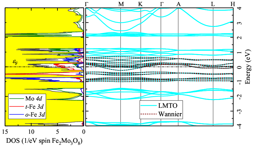
We use the linear muffin-tin orbital (LMTO) method LMTO1; LMTO2 and the experimental structure parameters reported in Ref. Fe2Mo3O8str. The practical aspects of calculations (including the choice of atomic sphere, etc.) can be found in Ref. LMTO_details. The corresponding band structure in LDA is shown in Fig. 2.
Some test calculations have been also performed using the full potential Wien2k method Wien2k, which reveals a good agreement with the LMTO results, as discussed in Supplemented Materials SM.
Owing to the trimerization of Mo kagome-like layers Wang_SciR, the Mo states form well separated groups of bands each of which corresponds to the particular type of molecular orbitals. This can be understood as follows. The formal configuration of octahedrally coordinated Mo4+ ions is . If intersite hybridization is larger than the crystal field, as in the Mo3 trimer, two orbitals ( and in Fig. 3) at each Mo site can be chosen so to form the maximal overlap with either or orbitals of the neighboring Mo site, where each orbital participates in the hybridization in only one Mo-Mo bond, as schematically illustrated in Fig. 3(b).

In reality, such hybridization can occur via the Mo-O-Mo paths of the edge sharing MoO6 octahedra, as shown in Fig. 3(a) or directly, as shown in Fig. 3(b). Therefore, in each of the Mo-Mo bonds, the atomic and orbitals will form bonding and antibonding molecular states, which are schematically shown in Fig. 3(c). Then, the third orbital ( in Fig. 3) will be nonbonding. In solids, these molecular levels will form bands, which can be still classified as bonding (at around eV in Fig. 2), nonbonding (at around eV), and antibonding (at around eV). Since the bonding-nonbonding-antibonding splitting is much larger than the Hund’s coupling (typically, about eV for Mo), the system will remain nonmagnetic with six electrons of the Mo3 trimer residing at the bonding orbitals.
The magnetic Fe bands, which are located near the Fermi level, in the energy interval of about eV, are sandwiched between bonding and nonbonding Mo bands. The Fe and Mo bands are separated from each other by a finite energy gap, which makes straightforward the construction of the effective model for the Fe bands. Furthermore, there are two groups of the Fe bands: the -Fe one, which is formed mainly by the tetrahedral sites and located closer to the Fermi level, and the -Fe bands, formed by the octahedral sites, which are split and located away from the Fermi level.
II.2 Effective model for the Fe bands
The effective Hubbard-type model for the magnetic Fe bands,
| (1) |
is formulated in the basis of the Wannier functions WannierRevModPhys, where () is the operator of creation (annihilation) of an electron at the orbital , , , , or of the Fe site with the spin or footnote1. The Wannier functions are constructed using the projector-operator technique and the orthonormal LMTO’s as the trial functions review2008.
The one-electron part of the model Hamiltonian, , is given by the matrix elements of the Kohn-Sham LDA Hamiltonian in the Wannier basis. Since the latter is complete in the subspace of the Fe bands, the obtained perfectly reproduces the original LDA bands in this region (Fig. 2) review2008. Then, the matrix elements of with stand for the transfer integrals, while the ones with describe the crystal-field effects.
The scheme of atomic level splitting (the eigenvalues of for ) is shown in Fig. 4.

As expected, the levels are split into the triply-degenerate and doubly-degenerate states. In the tetrahedral environment, the states are located lower in energy, while in the octahedral one the order of the and levels is reversed. The - splitting () is about and meV at the -Fe and -Fe sites, respectively, which is reasonable agreement with the results of the Wien2k calculations ( and meV, respectively). The splitting is substantially larger at the -Fe sites, which is consistent with the form of LDA density of states in Fig. 2, where the -Fe states are located near the Fermi level and sandwiched by the -Fe states from below and above. In the hexagonal P63mc symmetry, the levels are further split into non-degenerate and doubly-degenerate states by about and meV at the -Fe and -Fe sites, respectively (where the states are located lower in energy). The Wien2k method provides somewhat different scheme of the level splitting: and meV at the -Fe and -Fe sites, respectively, where the lower energy level is of the symmetry. The difference is related to the asphericity of the Kohn-Sham potential in the Wien2k method. Nevertheless, some portion of this asphericity (and, therefore, the crystal-field splitting) should be subtracted in order to avoid the double-counting problem in the process of solution of the Hubbard model (1), which also includes the nonspherical effects, of the same origin, driven by the screened on-site Coulomb interaction review2008. Fortunately, the level splitting is not particularly large and does not affect our finite results: in numerical calculations we used two schemes of the level splitting, obtained in LMTO and Wien2k, and both of them yielded similar conclusion regarding the form of the orbital ordering and interatomic exchange interactions.
Thus, from the viewpoint of symmetry and atomic level splitting, one can expect the following scenaria. First of all, the majority-spin states of -Fe and -fe will be fully occupied. Then, 2 minority-spin electrons can reside at the low-lying orbitals of -Fe, resulting in the charge-disproportionated solution , which respects the P63mc symmetry of Fe2Mo3O8. It may look at odds with the scheme of crystal-field splitting (Fig. 4), where the orbitals of -Fe are located lower in energy and therefore are expected to be occupied first. However, we will see in a moment that the solution is also supported by the form of the screened on-site Coulomb interactions. In the case of homogeneous solution (the second scenario), each of the minority-spin electrons at the -Fe and -Fe sites will reside at the degenerate and orbitals, respectively, so that the system will tend to lift the degeneracy through the Jahn-Teller distortion and/or orbital ordering.
The parameters of screened on-site Coulomb interactions, , were calculated using simplified version of the constrained random-phase approximation (RPA) Ferdi04, as explained in Ref. review2008. Each matrix can be fitted in terms of the Coulomb repulsion , the intra-atomic exchange interaction , and the nonsphericity , where , , and are the screened radial Slater’s integrals JPSJ. The results of such fitting are shown in Table 1.
| -Fe | -Fe | |
|---|---|---|
One can see that the screened is relatively small. This is understandable considering the electronic structure of Fe2Mo3O8: the Fe bands are sandwiched by the Mo ones (Fig. 2), which also have a large weight of the Fe states and, therefore, very efficiently screen the Coulomb interactions in the target Fe bands review2008. Furthermore, the Coulomb is smaller at the tetrahedral sites. This is also closely related to the electronic structure of Fe2Mo3O8, where the -Fe bands are mainly located near the Fermi level, inside the -Fe ones: since the screening in RPA is governed by the electronic excitations between occupied and unoccupied states, the strongest effect is expected for those states, which are located near the Fermi level. The change of the Coulomb repulsion parameter between tetrahedral and orthorhombic sites, , is about eV, which does not seem to be large. Nevertheless, it corresponds to the change of the Coulomb potential eV for , which tends to drive the system into the charge disproportionation regime and formation of the electronic state instead of the charge homogeneous one .
II.3 Solution of the model
The model (1) was solved in the mean-field Hartree-Fock (HF) approximation review2008 for the AFM and FRM phases (see Fig. 5) as well as other magnetic configurations, which were used for the construction of the spin model SM.

The straightforward solution of the model (1) leads to the configuration, which is supported by the crystal-field splitting of the atomic levels and the values of the Coulomb repulsion at the -Fe and -Fe sites. The corresponding densities of states are shown in Fig. 6.

As expected, this solution is insulating: the band gap is about eV and formed between states of -Fe and states of -Fe.
Nevertheless, we do not rule out the possibility that the obtained charge-disproportionated solution may also be an artifact of calculations, because our model (1) does not include the double-counting term LDAU. The double-counting term typically serve to subtract the portion of Coulomb and exchange-correlation interactions, which are already included at the level of LDA/GGA (the generalized gradient approximation) LDAU. In the homogeneous case with one type of correlated ions, this correction is reduced to the constant energy shift and, therefore, can be neglected, since calculating the Fermi level we restore status quo. However, if the screened Coulomb repulsion is different at different atomic sites, as in the case of the -Fe and -Fe, such correction can be important.
Therefore, we have also considered the homogeneous solution , which can be obtained in constraint calculations fixing the number of electrons at the -Fe and -Fe sites. In fact, the original LDA calculations, where no sizable charge disproportionation have been detected (Fig. 2), also speak in favor of such homogeneous solution. The corresponding densities of states for the AFM and FRM phases are shown in Fig. 7.

In this case, the on-site Coulomb interactions lift the orbital degeneracy of the -Fe and -Fe levels through the formation of the orbitally ordered state, which breaks the P63mc symmetry, opens the bang gap of about eV, and minimizes the energy of interatomic exchange interactions KugelKhomskii.
In order to visualise this orbital ordering, we plot the density formed by one minority-spin electron around each Fe site, which was obtained by integrating the states in the energy window eV in Fig. 7. The results are shown in Fig. 8 for the AFM and FRM phases.


As expected, the change of the spin order from AFM to FRM leads to the change of the orbital order and the spacial reorientation of the occupied minority-spin orbitals so to further stabilize the given spin order KugelKhomskii. Loosely speaking, the AFM coupling between nearest-neighbor sites along the axis, realized in the FRM phase, coexists with the “ferro” orbital order, where the occupied minority-spin orbitals in the bond are oriented in a similar way. On the contrary, the ferromagnetic coupling along in the AFM phase coexists with the “antiferro” orbital order, where the occupied orbitals form some angle with respect to each other. In other words, in the FRM case the system tends to fill the same orbitals for -Fe and -Fe along in order to minimize the energy of superexchange interactions between these and other orbitals, which have considerable overlap.
Finally, we note that the FRM solution corresponds to the compensated ferrimagnetic case, where the -Fe and -Fe sublattices are inequivalent, but the net spin magnetic moment is equal to zero.
II.4 Interatomic exchange interactions
The interatomic exchange interactions can be evaluated by mapping the total energy change caused by the reorientation of spins onto the Heisenberg model JHeisenberg:
| (2) |
where is the direction of spin at the site . In order to evaluate , we used two different techniques. The first one is based on finite rotations of spins, where is related to the total energies of several collinear magnetic configurations obtained by aligning each of the four Fe spins in the unit cell either up or down. The method is standard and widely used in electronic structure community for the analysis of the magnetic properties.
The second method is based on the infinitesimal rotations of spins near the equilibrium, where are obtained in the second order perturbation theory with respect to the rotations of the self-consistent HF potentials at the sites and JHeisenberg; review2008:
| (3) |
Here, is the one-electron Green’s for the majority and minority spin states, is the spin part of the HF potential at the site , is the Fermi energy, and denotes the trace over the orbital indices. Generally, the parameters calculated using the second technique depend on the magnetic state, thus reflecting the change of the electronic structure and the orbital ordering. The comparison of such parameters, calculated in different magnetic states, presents a test for the validity of the Heisenberg model, which can be defined locally, for the infinitesimal spin rotations, but not necessary globally, to describe the energies of all possible spin configurations where each spin can have an arbitrary direction, irrespectively on the direction of its neighboring spins.
The results of Green’s function calculations are summarized in Fig. 9 and the main exchange interactions are explained in Fig. 1.

Somewhat surprisingly, the exchange interactions exhibit quite similar behavior for the solutions and . Furthermore, we note the following: (i) The orbital ordering accompanying the solution for the AFM and FRM states lowers the P63mc symmetry. Such symmetry lowering is manifested in somewhat different values of the exchange parameters, which are realized in the crystallographically equivalent bonds, as is clearly seen for , and in the lower panel of Fig. 9. Nevertheless, this difference is not particularly large (for instance, in comparison with the difference between , , and other interactions). Therefore, in the first approximation one can average the exchange parameters over the crystallographically equivalent bonds and neglect the difference between them. Such problem does not occurs for the solution , which respects the P63mc symmetry; (ii) Apart from the symmetry lowering, which can be different for the AFM and FRM states reflecting the difference in the orbital ordering, the averaged parameters reveal very similar behavior for the AFM and FRM states SM; (iii) Very similar set of exchange parameters can be obtained by mapping the energies of collinear magnetic configurations and flipping each spin instead of rotating it by an infinitesimal angle (Table 2).
| () | () | () | () | |
| () | () | () | () |
These arguments suggest that the spin model (2) is well defined and can be used for the analysis magnetic properties of Fe2Mo3O8 in the wide temperature range.
All are antiferromagnetic. The AFM coupling between -Fe and -Fe in each layer is stabilized by , which is the strongest interaction in the system. The magnetic ordering between the layers results from the competition of three main interactions: the nearest-neighbor (nn) interaction between -Fe and -Fe, together with , tends to stabilize the FRM phase, while the next-nn interactions and operating, respectively, in the sublattices -Fe and -Fe favor (again, together with ) the AFM alignment. Furthermore, the effect of is strengthened by 2nd neighbor interactions between -Fe and -Fe: although is considerably smaller, the number of such bonds is large (see Fig. 1), making the total contribution comparable with . Thus, the relevant parameter responsible for the emergence of the FRM order is . Considering the numbers of bonds, one can find the following condition for the stability of the AFM phase relative to the FRM one: , which is satisfied for both and . Nevertheless, the AFM structure is not the ground state of the model: the competition of , , and () should lead to the noncollinear magnetic order with the propagation vector close to SM. It would be interesting to chesk this point experimentally. Finally, the exchange interaction is considerably weaker than , which has important consequences on the magnetic properties of Fe2Mo3O8: with the increase of the temperature (), the magnetization in the -Fe sublattice will tend to vanish faster than in the -Fe one (which is quite expected for the systems with different magnetic sublattices CoV2O4). Therefore, even for the homogeneous solution , where the net magnetization is zero at , both in the AFM and FRM case, one can expect appearance of finite net magnetization at finite , which couples to the magnetic field and can be used for the switching between the AFM and FRM phases.
II.5 Parameters of electric polarization
We assume that the magnetic part of the electric polarization parallel to the axis can be described by the following expression:
| (4) |
which is similar to Eq. (2) for the exchange interaction energy. In principle, Eq. (4) can be derived rigorously, by applying the Berry-phase theory of electric polarization FE_theory to the model (1) PRB2012 and considering the limit of large , as is typically done in the theories of double exchange and superexchange interactions for the spin Hamiltonian (2) without spin-orbit coupling PRB2014; PRB2019. Nevertheless, since interatomic exchange interactions are well reproduced by mapping the total energies obtained in the self-consistent Hartree-Fock calculations for a limited number of magnetic configuration, we employ here a similar strategy for and derive the parameters by mapping the values of electric polarization obtained in the same calculations onto Eq. (4) and assuming that, similar to , the main details of can be described by four independent parameters: , , , and . They are listed in Table 3.
Unlike , the parameters differ substantially in the case of and . In the former case, all parameters are large and equally important, while in the latter case clearly prevails. Somewhat unexpectedly, we have found large for charge disproportionated configuration . Indeed, is proportional to (the difference of atomic -coordinates in the bond), which is rather small for the nn in-plane bonds (about Å). On the other hand, the ionic charge difference between -Fe1+ and -Fe3+ is large, which readily compensates the smallness of . In the charge neutral regime, , is expectedly small (and is fully associated with the redistribution of the tails of the Wannier functions at the -Fe and -Fe sites PRB2014; PRB2019).
In principle, the model can be further extended to include antisymmetric and anisotropic effects driven by the relativistic spin-orbit coupling. The corresponding expressions can be found in Ref. PRB2019. However, since the magnetic transition takes place between two collinear configurations, AFM and FRM, it is reasonable to expect that the main contribution to the change of is isotropic and described by Eq. (4).
III Discussion
Much insight can be gained from the solution of the spin model (2) in the molecular-field approximation (MFA). Namely, the molecular field corresponding to the spin Hamiltonian (2) is given by
| (5) |
where is the relative magnetization at the site . Then, can be found from the temperature average of the spin operator in the molecular field :
| (6) |
where is the Brillouin function for the spin Mattis. The equations (5) and (6) are solved self-consistently and the Néel temperature () is defined as the minimal temperature for which . Then, the spin-dependent part of the polarization in the AFM state, the total energy difference between the FRM and AFM phases, and the polarization jump caused by the AMF-to-FRM transition can be evaluated as
| (7) |
| (8) |
and
| (9) |
respectively. Unless specified otherwise, we use the parameters listed in Tables 2 and 3. The results are summarized in Figs. 10 and 11.


The molecular field estimate for is about and K for and , respectively. Quite expectedly, similar sets of parameters (see Table 2) yield similar values of . Thus, from this point of view the solutions and are “indistinguishable”. More rigorous estimate for can be obtained by considering Tyablikov’s RPA tyab, generalized to the case of multiple magnetic sublattices TCRPA and noncollinear magnetic ground state SM, which is expected in both and models for Fe2Mo3O8 (see Sec. II.4). The RPA yields and K for and , respectively. The latter estimates are close to the experimental K Wang_SciR; Kurumaji_PRX, while the MFA values are typically overestimated. The large difference between the MFA and RPA is related to the existence of weakly dispersive regions of magnon energies, which are nearly degenerate with the ground state SM. We have also used the full set of parameters, obtained in the Green’s function calculations for (Fig. 9), which obeys the crystallographic P63mc symmetry. This yields slightly smaller value of and K in MFA and RPA, respectively. Thus, even though the MFA substantially overestimates , it is still interesting to explore the abilities of this approximation for the description of magnetoelectric properties of Fe2Mo3O8, at least on the semi-quantitative level.
Since , the magnetization in the -Fe and -Fe sublattice exhibits different temperature dependence, where tends to decrease more rapidly than with the increase of . Then, the temperature dependence of the net magnetization, , will be nonmonotonous, with some “optimal value” corresponding to the maximum of , for which one can achieve the largest energy gain caused by the interaction with the external magnetic field. This effect is especially important for , where the spins in the -Fe and -Fe sublattices exactly cancel each other at , thus excluding a linear coupling with the magnetic field. Nevertheless, at finite , such cancellation does not occur, giving rise to the net magnetization in each honeycomb layer, the direction of which can be controlled by the magnetic field so to cause the AFM-FRM transition.
The key question is whether the AFM-FRM transition can be induced by experimentally accessible magnetic field, , which depends on and varies from about at till at Wang_SciR; Kurumaji_PRX. Although theoretical , which can be estimated as , shows the same tendency, it is overestimated in comparison with the experiment: for instance, at our is about and further increases with the decrease of . One reason may be the overestimation of in MFA. Moreover, this has a maximum as a function : since decreases more rapidly, the last term in Eq. (8) starts to prevail at elevated and additionally stabilizes AFM order relative to the FRM one. This worsens the agreement with the experimental data for . Another reason is that we do not consider the lattice effects, assuming that the AFM and FRM phases are described by the same crystal structure, while in reality the lattice relaxation in the FRM phase will certainly decrease the value of .
Thus, from the viewpoint of magnetism, the main difference between the and scenarios is that in the former case remains finite even at small , leaving possibility of the AFM-FRM transition in the magnetic field. This could be checked experimentally and according to our estimates it will require .
The behavior of spin-dependent part of the electric polarization is sensitive to the charge state of the Fe ions. Since the parameters of polarization are generally smaller for the homogeneous state (see Table 3), is also smaller (by about factor 4 in comparison with ). The obtained C/cm2 in the model is comparable with the experimental value of about C/cm2 Wang_SciR. Nevertheless, the overall shape of is quite different: the experimental dependence exhibits the jump at , which may signal that the magnetic transition is accompanied by the structural one Wang_SciR, while the theoretical decreases steadily down to .
The theoretical for has a clear maximum at , similar to the behavior of (Fig. 10). This is because is the strongest parameter in the case of (see Table 3), which clearly dominates with the increase of when other contributions to Eq. (7) decrease due to more rapid decrease of . On the other hand, in is nearly monotonous function of : in this case, the effect of is partly compensated by , so that the temperature dependence of is mainly controlled by strong in the first term in Eq. (7). Thus, in principle, the temperature dependence of can be used to distinguish experimentally between the configurations and .
Nevertheless, both scenaria yield a comparable polarization jump , caused by the AFM-FRM transition near (see Fig. 11). First, does not depend on . Then, the effect of strong in the case of is compensated by and , which are also strong, while in the case of , is mainly controlled by . The value of at is about C/cm2, which is comparable with the experimental data Wang_SciR; Kurumaji_PRX. Finally, we note also that is positive while is negative, which is also consistent with the experimental situation.
IV Summary and Conclusions
The magnetic exchange interactions and the origin of giant magnetoelectric effect in Fe2Mo3O8 have been studied on the basis of microscopic toy model derived for the magnetic Fe states from the first-principles electronic structure calculations. In spites of its simplicity, the model provides rather rich physics and accounts for the magnetic properties of Fe2Mo3O8 on the semi-quantitative level. Particularly, we propose two scenaria for the magnetic behavior of Fe2Mo3O8. The first one is based on the homogeneous distribution of the Fe2+ ions amongst the - and -sites, while the second one involves the charge disproportionation Fe2+ Fe1+Fe3+ with somewhat exotic ionization state at the -sites. Both scenaria lead ro similar sets of interatomic exchange interactions, which are consistent with available experimental data and explain the origin of the AFM and FRM phases. The crucial test to distinguish between the and configurations is the net magnetization in the honeycomb layer at low , which is expected to vanish (and emerge only at elevated ) in the case of , but remains finite in the case of in the molecular-field approximation, thus giving a possibility to control this nagnetization and induce the AFM-FRM transition by applying magnetic field.
Our calculations reproduce the order of magnitude of the experimentally observed giant magnetoelectric effect in Fe2Mo3O8, which we attribute to the electronic polarization related to the change of the electronic structure depending on the magnetic state, but for the fixed crystal structure Picozzi. However, the quantitative description of the temperature dependence of the polarization change will probably require the lattice effects, as was suggested in Ref. Wang_SciR.
Another interesting problem, which was not addressed in the present work, is the effects of relativistic spin-orbit (SO) interaction and the orbital magnetism, which are expected to play an important role especially in the configuration with the orbital degeneracy. Nevertheless, the problem is rather complex to be systematically studied in the present publication. Briefly, in the case of , our mean-field HF calculations for the available experimental P63mc structure with the SO coupling yield unquenched orbital moment of about at the -Fe sites, which has the same direction as the spin one, according to third Hund’s rule. The orbital moment at the -Fe sites is negligibly small as expected for the configuration. Thus, the orbital magnetization contributes to the net magnetic polarization in the honeycomb layer, though this contribution is not particularly strong in comparison with the spin one. In the case, the SO interaction lifts the orbital degeneracy lowering the P63mc symmetry and resulting in the canted spin state. In the ground state, the canting is such that the () components of magnetic moments are ordered as AFM, while the () components form the FRM structure. Beside spin, we also expect the orbital magnetization of the order of at the -Fe and -Fe sites. Thus, if this scenario is correct, the AFM-FRM transition can be tuned continuously, by applying the magnetic field in the plane and thus tune the value of the electric polarization.
V Acknowledgements
We are grateful to D.-J. Huang, S.-W. Cheong, Z. Hu, A. Ushakov, S. Nikolaev, and D. Khomskii for valuable discussions. This work was supported by the Russian Science Foundation through RSF 17-12-01207 research grant.
References
- (1) Y. Haraguchi, C. Michioka, M. Imai, H. Ueda, and K. Yoshimura, Phys. Rev. B 92, 014409 (2015).
- (2) S. Yu, B. Gao, J. W. Kim, S.-W. Cheong, M. K. L. Man, J. Madéo, K. M. Dani, and D. Talbayev, Phys. Rev. Lett. 120, 037601 (2018).
- (3) J. P. Sheckelton, J. R. Neilson, D. G. Soltan, and T. M. Mcqueen, Nature Mater. 11, 493 (2012).
- (4) Y. Wang, G. L. Pascut, B. Gao, T. A. Tyson, K. Haule, V. Kiryukhin, and S.-W. Cheong, Sci. Rep. 5, 12268 (2015).
- (5) T. Kurumaji, S. Ishiwata, and Y. Tokura, Phys. Rev. X 5, 031034 (2015).
- (6) G. Chen and P. A. Lee, Phys. Rev. B 97, 035124 (2018).
- (7) S. V. Streltsov and D. I. Khomskii, Physics-Uspekhi 60, 1121 (2017).
- (8) A. Sasaki, S. Yui, M. Yamaguchi, Mineral. J. 12, 393 (1985).
- (9) Y. Le Page and P. Strobel, Acta Crystallographica Section B 38, 1265 (1982).
- (10) H. Czeskleba, P. Imbert, and F. Varret, AIP Conf. Proc. 5, 811 (1972).
- (11) D. Bertrand and H. Kerner-Czeskleba, Le J. Phys. Colloq. 36, 379 (1975).
- (12) T. Kurumaji, Y. Takahashi, J. Fujioka, R. Masuda, H. Shishikura, S. Ishiwata, and Y. Tokura, Phys. Rev. B 95, 020405(R) (2017).
- (13) T. Kurumaji, Y. Takahashi, J. Fujioka, R. Masuda, H. Shishikura, S. Ishiwata, and Y. Tokura, Phys. Rev. Lett. 119, 077206 (2017).
- (14) T. N. Stanislavchuk, G. L. Pascut, A. P. Litvinchuk, Z. Liu, S. Choi, M. J. Gutmann, B. Gao, K. Haule, V. Kiryukhin, S.-W. Cheong, A. A. Sirenko, arXiv:1902.02325.
- (15) Y. Li, G. Gao, and K. Yao, Europhys. Lett. 118, 37001 (2017).
- (16) I. V. Solovyev, P. H. Dederichs, and V. I. Anisimov, Phys. Rev. B 50, 16861 (1994).
- (17) I. V. Solovyev and K. Terakura, Phys. Rev. B 58, 15496 (1998).
- (18) O. K. Andersen, Phys. Rev. B 12, 3060 (1975).
- (19) O. Gunnarsson, O. Jepsen, and O. K. Andersen, Phys. Rev. B 27, 7144 (1983).
- (20) https://www2.fkf.mpg.de/andersen/LMTODOC/LMTODOC.html
- (21) P. Blaha, K. Schwarz, G. K. H. Madsen, D. Kvasnicka, J. Luitz, R. Laskowski, F. Tran, and L. D. Marks, WIEN2k, An Augmented Plane Wave + Local Orbitals Programfor Calculating Crystal Properties (Karlheinz Schwarz, Techn. Universität Wien, Austria, 2018).
- (22) See Supplemented Material for the electronic structure in Wien2k, mapping of total energies and electric polarizations onto the isotropic spin model, magnetic state dependence of exchange interactions, spin-wave dispertion in the antiferromagnetic state, and the random-phase approximation for the critical temperature.
- (23) C. J. Bradley and A. P. Cracknell, The Mathematical Theory of Symmetry in Solids (Clarendon Press, Oxford, 1972).
- (24) N. Marzari, A. A. Mostofi, J. R. Yates, I. Souza, and D. Vanderbilt, Rev. Mod. Phys. 84, 1419 (2012).
- (25) All model parameters are available upon request.
- (26) I. V. Solovyev, J. Phys.: Condens. Matter 20, 293201 (2008).
- (27) F. Aryasetiawan, M. Imada, A. Georges, G. Kotliar, S. Biermann, and A. I. Lichtenstein, Phys. Rev. B 70, 195104 (2004).
- (28) I. Solovyev, J. Phys. Soc. Jpn. 78, 054710 (2009).
- (29) K. I. Kugel and D. I. Khomskii, Sov. Phys. Usp. 25, 231 (1982).
- (30) A. I. Liechtenstein, M. I. Katsnelson, V. P. Antropov, and V. A. Gubanov, J. Magn. Magn. Matter. 67, 65 (1987).
- (31) N. Menyuk, K. Dwight, and D. G. Wickham, Phys. Rev. Lett. 4, 119 (1960).
- (32) R. D. King-Smith and D. Vanderbilt, Phys. Rev. B 47, 1651 (1993); D. Vanderbilt and R. D. King-Smith, ibid. 48, 4442 (1993); R. Resta, J. Phys.: Condens. Matter 22, 123201 (2010).
- (33) I. V. Solovyev, M. V. Valentyuk, and V. V. Mazurenko, Phys. Rev. B 86, 144406 (2012).
- (34) I. V. Solovyev and S. A. Nikolaev, Phys. Rev. B 90, 184425 (2014).
- (35) S. A. Nikolaev and I. V. Solovyev, Phys. Rev. B 99, 100401(R) (2019).
- (36) D. C. Mattis, The Theory of Magnetism Made Simple (World Scientific, Singapore, 2006)
- (37) S. V. Tyablikov, Methods of Quantum Theory of Magnetism, Nauka, Moscow, (1975).
- (38) J. Rusz, I. Turek, and M. Diviš, Phys. Rev. B 71, 174408 (2005).
- (39) S. Picozzi, K. Yamauchi, B. Sanyal, I. A. Sergienko, and E. Dagotto, Phys. Rev. Lett. 99, 227201 (2007).