Towards Diverse and Accurate Image Captions via Reinforcing Determinantal Point Process
Abstract
Although significant progress has been made in the field of automatic image captioning, it is still a challenging task. Previous works normally pay much attention to improving the quality of the generated captions but ignore the diversity of captions. In this paper, we combine determinantal point process (DPP) and reinforcement learning (RL) and propose a novel reinforcing DPP (R-DPP) approach to generate a set of captions with high quality and diversity for an image. We show that R-DPP performs better on accuracy and diversity than using noise as a control signal (GANs, VAEs). Moreover, R-DPP is able to preserve the modes of the learned distribution. Hence, beam search algorithm can be applied to generate a single accurate caption, which performs better than other RL-based models.
1 Introduction
Image captioning, which combines the fields of computer vision (CV) and natural language processing (NLP), is a challenging task, which has drawn much attention from the two communities and significant progress has been achieved. Earlier works Kulkarni et al. 2013; Farhadi et al. 2010; Fang et al. 2015 generally directly employ vision and language models. However, these two-stage models cannot be trained in a end-to-end manner, which limits their performance.
Recently, CNN-LSTM models have become popular Vinyals et al. 2015; Xu et al. 2015. CNN-LSTM models are typically composed of three modules: (1) a visual CNN, (2) a language LSTM, and (3) the connection module between them, which can be trained in an end-to-end manner. More powerful captioning models are later proposed Anderson et al. 2017; Rennie et al. 2017; Wang et al. 2019, and trained using reinforcement learning (RL) where the evaluation metric (e.g., CIDEr) is used as the reward function. As a result, the generated captions obtain high quality according to the most popular metrics, such as BLEU Papineni et al. 2002, METEOR Denkowski and Lavie 2014, ROUGLE Lin 2004, CIDEr Vedantam et al. 2015 and SPICE Anderson et al. 2016.
However, most of the above models do not focus on the diversity of captions. While directly maximizing the metrics using RL Rennie et al. 2017 significantly improves the metric scores, they lack diversity even though they are randomly drawn from the learned distribution Wang and Chan 2019. The lack of diversity in the captions is further exacerbated when using beam search to find the mode of the learned distribution.
The main issue of RL-based methods that leads to generating less diverse captions is they only consider the quality (as measured by BLEU or CIDEr) of samples during training. To address this issue, in this paper, we propose a novel approach that combines RL and determinantal point processes (DPP) Kulesza and Taskar 2012 that generates both accurate and diverse image captions. Inspired by DPPs, which account for the quality and diversity of subsets, we first propose a new metric that is able to reflect the quality and diversity of a set of captions. We then maximize the proposed metric score using RL, which is equivalent to a DPP training process. We evaluate our model using the diversity metrics from Wang and Chan 2019, and our proposed R-DPP model achieves both high accuracy and high diversity scores. In addition, R-DPP preserves the modes of the learned distribution – applying the beam search algorithm to generate one high-quality caption yields better performance than the baseline captioning model. Moreover, R-DPP outperforms its counterparts on the oracle test (see Table 2).
2 Related Work
Diverse image captioning.
Recently, generating diverse captions receives much attention, and a variety of captioning models are developed, such as CVAE Wang et al. 2017, CGAN Dai et al. 2017, GroupTalk Wang et al. 2016, GroupCap Chen et al. 2018a, POS Deshpande et al. 2018 and SCT Cornia et al. 2018. CVAE and CGAN employ random noise vectors to control the difference among the generated captions. However, the diversity is highly related to the variance of the noise, which makes it difficult to balance diversity and accuracy. GroupTalk employ multiple captioners11 1 A captioner could be a captioning model. and a classifier to generated diverse captions. Each captioner generate one caption and the classifier is used to control the diversity among the captions. However the computational cost is high due to its use of multiple captioners. GroupCap considers the structure relevance and diversity constraint to generate both accurate and diverse captions, in which VP-trees are constructed. POS introduces part-of-speech (POS) tags to control the difference among captions, which contains two branches: 1) POS tag prediction, 2) word prediction. The same POS tag could result in using different words (synonyms), leading to diversity. Instead of employing POS tags as control signals, SCT applies noun chunks that are obtained by dependency parsing Chen and Manning 2014. Compared with the above captioning models, our proposed RL using DPP is much simpler and more efficient, does not require any other branches or control signals, and can be applied to any baseline captioning model.
Determinantal point process (DPP).
Given a discrete set , a DPP measures the probability of each subset of , which is defined as Kulesza and Taskar 2012:
| (1) |
where is a positive semidefinite matrix, representing an L-ensemble, denotes the identity matrix and .
Generally, can be decomposed as a Gram matrix with elements , where denotes the quality of the th element and denotes the similarity between the th and th elements, where .
A DPP is trained by maximizing the log-likelihood , where the subset with larger will be assigned a higher probability. Inference involves finding the subset with highest posterior probability (MAP). DPP has been used in applications that require both quality and diversity: text summarization Kulesza and Taskar 2012, video summarization Zhang et al. 2016, recommendation Chen et al. 2018b and neural conversation Song et al. 2018.
3 DPP-based Reinforcement Learning for Image Captioning
We consider each caption as an item, and define the quality of a caption using CIDEr,
| (2) |
where denotes the th caption in a subset, denotes human annotations and is the CIDEr score. We define the similarity between captions as (i.e., “self-CIDEr” in Wang and Chan 2019),
| (3) |
The matrix in DPP is then
| (4) |
where , , and denotes element-wise multiplication.
Let be the captioning model and a subset of captions sampled from . The probability of can be measured with (1), using the determinants of and . Unfortunately, to compute is intractable since the number of possible captions is huge, roughly , where is the dictionary size (10,000) and is the caption length (16). Although computing is intractable, we note that is a constant w.r.t. for a fixed dictionary and caption length . Thus, the denominator in (1) can be ignored when maximizing the likelihood of the generated captions w.r.t. ,
To compute the quality scores and similarity matrix, we should sample a set of captions from , and thus we cannot directly calculate the gradient of w.r.t. . Alternatively, we can first compute the derivative , where is the element of and is the element of .22 2 Adding a small constant to ensures invertability. Considering the derivative , its sign indicates whether we should reduce or increase to enlarge .
Recall that the reward function in Rennie et al. 2017 is the expectation of CIDEr,
| (5) |
and the corresponding policy gradient is
| (6) |
(6) shows that the probability of the high-quality captions will increase, and finally the model could tend to generate captions that have high quality but lack diversity.
The main issue of using (5) is that it only accounts for the quality of captions. To promote diversity, we employ a new reward function that considers each pair of captions in ,
| (7) |
where is the sign of , and is the probability of the th caption according to . Note that is the joint probability of the th and th captions, since the captions are sampled independently. Our reward function considers both the quality of captions as well as the similarity among captions (see Eq. (4))33 3 Note that the expectation of could be enlarged or reduced based on , which is different with Eq. (5) where the expectation of is always enlarged., thus is able to balance the quality and diversity. The corresponding policy gradient is (see supplemental for derivation):
| (8) | ||||
which has the same form as (6), but here we consider both quality and similarity among captions.
4 Experiments
Experimental setup.
We conduct our experiments on MSCOCO dataset, which has 123,287 annotated images, each with at least 5 captions. Following Rennie et al. 2017, we use 5k images for validation, 5k for testing and the remaining for training. Our baseline captioning model is based on Att2in Rennie et al. 2017. We first train the model for 100 epochs using cross-entropy loss, and then refine it for another 100 epochs using our policy gradient in (8). During training, we apply Adam with learning rate 0.0004. For comparison, we also refine the baseline model for 100 epochs using original policy gradient in (6). We also compare with CGAN44 4 We train CGAN without using rollout, which is different from Dai et al. 2017, GMM-CVAE Wang et al. 2017, SCST Rennie et al. 2017, and XE+CIDEr Wang and Chan 2019. The diversity metric is self-CIDEr diversity, which is shown to be more correlated to human judgment Wang and Chan 2019.
Results.

| Model | B-4 | M | R | C | S | |
|---|---|---|---|---|---|---|
| Adaptive-XE Lu et al. 2017 | 3 | 0.332 | 0.266 | - | 1.085 | - |
| Updown-XE Anderson et al. 2017 | 5 | 0.362 | 0.270 | 0.564 | 1.135 | 0.203 |
| Updown-RL Anderson et al. 2017 | 5 | 0.363 | 0.277 | 0.569 | 1.201 | 0.214 |
| DISC-RL Luo et al. 2018 | 2 | 0.363 | 0.273 | 0.571 | 1.141 | 0.211 |
| Hieratt-XE Wang et al. 2019 | 3 | 0.362 | 0.275 | 0.566 | 1.148 | 0.206 |
| Hieratt-RL Wang et al. 2019 | 3 | 0.376 | 0.278 | 0.581 | 1.217 | 0.215 |
| SCST Rennie et al. 2017 | - | 0.333 | 0.263 | 0.553 | 1.114 | - |
| Att2in-XE Rennie et al. 2017 | - | 0.313 | 0.260 | 0.543 | 1.013 | - |
| XE+5CIDEr Wang and Chan 2019 | 3 | 0.382 | 0.277 | 0.579 | 1.172 | 0.206 |
| XE+10CIDEr Wang and Chan 2019 | 3 | 0.378 | 0.276 | 0.580 | 1.174 | 0.207 |
| XE+20CIDEr Wang and Chan 2019 | 3 | 0.375 | 0.276 | 0.579 | 1.173 | 0.209 |
| Our R-DPP () | 3 | 0.371 | 0.279 | 0.579 | 1.222 | 0.214 |
| Our R-DPP () | 3 | 0.369 | 0.278 | 0.577 | 1.216 | 0.214 |
| Our R-DPP () | 3 | 0.360 | 0.280 | 0.572 | 1.198 | 0.214 |
| Our R-DPP () | 3 | 0.357 | 0.278 | 0.568 | 1.179 | 0.212 |
| Our R-DPP () | 3 | 0.352 | 0.276 | 0.566 | 1.146 | 0.208 |
| Our R-DPP () | 3 | 0.347 | 0.272 | 0.562 | 1.124 | 0.206 |
| Model | # | B-4 | M | R | C |
|---|---|---|---|---|---|
| AG-CVAE Wang et al. 2017 | 20 | 0.471 | 0.309 | 0.638 | 1.308 |
| GMM-CVAE Wang et al. 2017 | 20 | 0.449 | 0.299 | 0.624 | 1.251 |
| POS Deshpande et al. 2018 | 20 | 0.449 | 0.365 | 0.678 | 1.468 |
| SCT Cornia et al. 2018 | 20 | 0.448 | 0.366 | 0.689 | 1.565 |
| SCST Rennie et al. 2017 | 20 | 0.332 | 0.322 | 0.630 | 1.383 |
| Att2in-XE Rennie et al. 2017 | 20 | 0.329 | 0.326 | 0.621 | 1.216 |
| XE+5CIDEr Wang and Chan 2019 | 20 | 0.462 | 0.372 | 0.682 | 1.512 |
| XE+10CIDEr Wang and Chan 2019 | 20 | 0.465 | 0.372 | 0.689 | 1.568 |
| XE+20CIDEr Wang and Chan 2019 | 20 | 0.427 | 0.359 | 0.673 | 1.525 |
| Our R-DPP () | 10 | 0.407 | 0.349 | 0.659 | 1.495 |
| 20 | 0.443 | 0.365 | 0.677 | 1.563 | |
| Our R-DPP () | 10 | 0.442 | 0.367 | 0.677 | 1.567 |
| 20 | 0.494 | 0.388 | 0.702 | 1.656 | |
| Our R-DPP () | 10 | 0.455 | 0.374 | 0.686 | 1.585 |
| 20 | 0.518 | 0.400 | 0.713 | 1.691 | |
| Our R-DPP () | 10 | 0.463 | 0.375 | 0.688 | 1.585 |
| 20 | 0.527 | 0.405 | 0.717 | 1.700 | |
| Our R-DPP () | 10 | 0.458 | 0.374 | 0.686 | 1.585 |
| 20 | 0.528 | 0.403 | 0.718 | 1.690 | |
| Our R-DPP () | 10 | 0.452 | 0.373 | 0.683 | 1.545 |
| 20 | 0.529 | 0.404 | 0.718 | 1.684 |
Fig. 1 shows the performance of different models in the diversity-accuracy space. Human annotations achieve relatively high diversity and accuracy55 5 The accuracy score of human annotations is the leave-one-out CIDEr score as in Wang and Chan 2019., and there is still a large gap between the proposed models and human annotations. Our R-DPP model slightly improves the accuracy of SCST and the baseline model (Att2in), when , but the diversity score roughly doubles (0.2 to 0.4). Our R-DPP achieves comparable diversity scores as XE+CIDEr, but the captions generated by XE+CIDEr have lower accuracy compared to R-DPP. By maximizing , our R-DPP can simultaneously improves the quality and suppresses the similarity among captions (improves diversity). Comparing GMM-CVAE and R-DPP, both methods can generate captions with similar diversity, while R-DPP () has higher accuracy (0.8 vs 0.95), which indicates that R-DPP better approximates the modes of the ground-truth distribution. Finally, the R-DPP curve shows that the number of samples used during training balances the diversity and accuracy of the model. A larger leads to a more diverse set of captions, although it also incurs higher training computational cost.
Another advantage of R-DPP is that it can be used to generate a single high-quality caption for an image. Table 1 shows the comparison between R-DPP and the state-of-the-art models. Compared with SCST, R-DPP improves the CIDEr score from 1.114 to 1.222, and the other metric scores are also improved by around 5% or larger. Comparing with Hieratt-RL (state-of-the-art), R-DPP obtains similar CIDEr score, however, the Hieratt model cannot generate diverse captions.
Fig. 1 and Table 1 show the effectiveness of R-DPP on generating both diverse and accurate captions, whereas they do not consider the optimal selection of . Hence, we conduct experiments on oracle test (see Table 2)—the upper bound of each metric. R-DPP outperforms other methods, providing the highest-quality caption based on generating 20 captions. Even sampling 10 captions, R-DPP obtains higher scores. With the increase of , the scores increase in the beginning, but then fall, e.g., when we sample 20 captions, CIDEr score rises from 1.563 to 1.700 when increases from 2 to 5, after that it falls to 1.684. Also, when we sample 10 captions, R-DPP() performs better. Thus, using could be a better choice to well balance diversity and accuracy, which also obtains the highest-quality caption. We show more qualitative examples in the supplemental.
5 Conclusion
We have presented the reinforcing DPP (R-DPP) model, which is a simpler but efficient method for training a caption model to generate both diverse and accurate captions. Compared with other models, R-DPP obtains similar diversity score, but much higher accuracy score. In addition, the state-of-the-art oracle performance is significantly improved by R-DPP. In the future, we believe that more quality and diversity measurements should be introduced into R-DPP. It is also possible to extend R-DPP to other text generation tasks, such as dialog and machine translation, in order to provide diverse high-quality choices to the users.
References
- Anderson et al. (2016) Peter Anderson, Basura Fernando, Mark Johnson, and Stephen Gould. 2016. Spice: Semantic propositional image caption evaluation. In ECCV.
- Anderson et al. (2017) Peter Anderson, Xiaodong He, Chris Buehler, Damien Teney, Mark Johnson, Stephen Gould, and Lei Zhang. 2017. Bottom-up and top-down attention for image captioning and vqa. arXiv preprint arXiv:1707.07998.
- Chen and Manning (2014) Danqi Chen and Christopher Manning. 2014. A fast and accurate dependency parser using neural networks. In EMNLP, pages 740–750.
- Chen et al. (2018a) Fuhai Chen, Rongrong Ji, Xiaoshuai Sun, Yongjian Wu, and Jinsong Su. 2018a. Groupcap: Group-based image captioning with structured relevance and diversity constraints. In CVPR.
- Chen et al. (2018b) Laming Chen, Guoxin Zhang, and Eric Zhou. 2018b. Fast greedy map inference for determinantal point process to improve recommendation diversity. In NIPS, pages 5622–5633.
- Cornia et al. (2018) Marcella Cornia, Lorenzo Baraldi, and Rita Cucchiara. 2018. Show, control and tell: A framework for generating controllable and grounded captions. CoRR, abs/1811.10652.
- Dai et al. (2017) Bo Dai, Sanja Fidler, Raquel Urtasun, and Dahua Lin. 2017. Towards diverse and natural image descriptions via a conditional gan. In ICCV.
- Denkowski and Lavie (2014) M. Denkowski and A. Lavie. 2014. Meteor universal: Language specific translation evaluation for any target language. In EACL Workshop on Statistical Machine Translation.
- Deshpande et al. (2018) Aditya Deshpande, Jyoti Aneja, Liwei Wang, Alexander Schwing, and David A Forsyth. 2018. Diverse and controllable image captioning with part-of-speech guidance. arXiv preprint arXiv:1805.12589.
- Fang et al. (2015) Hao Fang, Saurabh Gupta, Forrest Iandola, Rupesh K. Srivastava, Li Deng, Piotr Dollar, Jianfeng Gao, Xiaodong He, Margaret Mitchell, John C. Platt, C. Lawrence Zitnick, and Geoffrey Zweig. 2015. From captions to visual concepts and back. In CVPR.
- Farhadi et al. (2010) Ali Farhadi, Mohsen Hejrati, Mohammad Amin Sadeghi, Peter Young, Cyrus Rashtchian, Julia Hockenmaier, and David Forsyth. 2010. Speaking the same language: Matching machine to human captions by adversarial training. In ECCV.
- Kulesza and Taskar (2012) Alex Kulesza and Ben Taskar. 2012. Learning determinantal point processes. arXiv preprint arXiv:1202.3738.
- Kulkarni et al. (2013) G. Kulkarni, V. Premraj, V. Ordonez, S. Dhar, S. Li, Y. Choi, A. C. Berg, and T. L. Berg. 2013. Babytalk: Understanding and generating simple image descriptions. IEEE Transactions on Pattern Analysis and Machine Intelligence, 35(12):2891–2903.
- Lin (2004) C.-Y. Lin. 2004. Rouge: A package for automatic evaluation of summaries. In ACL Workshop.
- Lu et al. (2017) Jiasen Lu, Caiming Xiong, Devi Parikh, and Richard Socher. 2017. Knowing when to look: Adaptive attention via a visual sentinel for image captioning. In CVPR.
- Luo et al. (2018) Ruotian Luo, Brian Price, Scott Cohen, and Gregory Shakhnarovich. 2018. Discriminability objective for training descriptive captions. In CVPR.
- Papineni et al. (2002) K. Papineni, S. Roukos, T. Ward, and W.-J. Zhu. 2002. Bleu: a method for automatic evaluation of machine translation. In ACL.
- Rennie et al. (2017) Steven J Rennie, Etienne Marcheret, Youssef Mroueh, Jerret Ross, and Vaibhava Goel. 2017. Self-critical sequence training for image captioning. In CVPR.
- Song et al. (2018) Yiping Song, Rui Yan, Yansong Feng, Yaoyuan Zhang, Dongyan Zhao, and Ming Zhang. 2018. Towards a neural conversation model with diversity net using determinantal point processes. In AAAI.
- Vedantam et al. (2015) R. Vedantam, C. Lawrence Zitnick, and D. Parikh. 2015. Cider: Consensus-based image description evaluation. In CVPR.
- Vinyals et al. (2015) Oriol Vinyals, Alexander Toshev, Samy Bengio, and Dumitru Erhan. 2015. Show and tell: A neural image caption generator. In CVPR.
- Wang et al. (2017) Liwei Wang, Alexander Schwing, and Svetlana Lazebnik. 2017. Diverse and accurate image description using a variational auto-encoder with an additive gaussian encoding space. In NIPS.
- Wang and Chan (2019) Qingzhong Wang and Antoni B. Chan. 2019. Describing like humans: on diversity in image captioning. CoRR, abs/1903.12020.
- Wang et al. (2019) Weixuan Wang, Zhihong Chen, and Haifeng Hu. 2019. Hierarchical attention network for image captioning. In AAAI.
- Wang et al. (2016) Zhuhao Wang, Fei Wu, Weiming Lu, Jun Xiao, Xi Li, Zitong Zhang, and Yueting Zhuang. 2016. Diverse image captioning via grouptalk. In IJCAI, pages 2957–2964. AAAI Press.
- Xu et al. (2015) Kelvin Xu, Jimmy Ba, Ryan Kiros, Kyunghyun Cho, Aaron Courville, Ruslan Salakhudinov, Rich Zemel, and Yoshua Bengio. 2015. Show, attend and tell: Neural image caption generation with visual attention. In ICML.
- Zhang et al. (2016) Ke Zhang, Wei-Lun Chao, Fei Sha, and Kristen Grauman. 2016. Video summarization with long short-term memory. In ECCV, pages 766–782. Springer.
The supplemental is arranged as follows:
- •
Details of the gradient computation.
- •
Qualitative examples of diverse image captions.
Appendix A Gradient Computation
We show how to compute the policy gradient in Eq. (11) in our paper. Recall that the reward function is defined as follows:
| (9) |
Note that only is a function of , then we have
| (10) | ||||
| (11) | ||||
| (12) | ||||
| (13) | ||||
| (14) |
Since and are symmetric mtrices, we can derive Eq. (13) from Eq. (12). Note that for , hence, we obtain Eq (12) from Eq. (11).
Appendix B Qualitative Examples
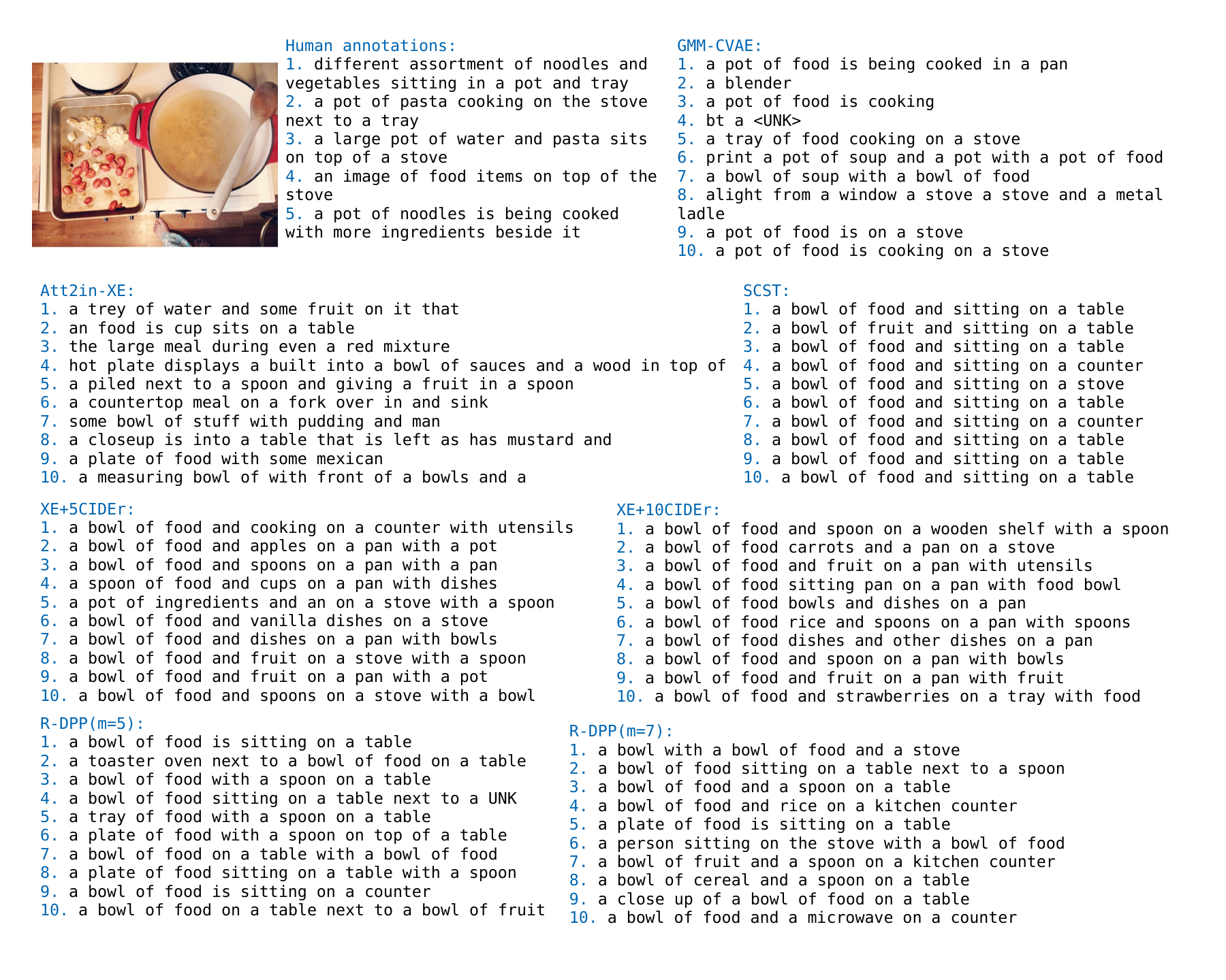
We show more qualitative results of R-DPP. Fig. 2 to 5 show the comparison between R-DPP and other models, and Fig. 6 to 9 show the generated captions by R-DPP with different numbers of samples during training. Compared with other methods, our R-DPP could generate more fluent and diverse captions. We find that R-DPP is able to generate captions with different sentence structures (syntactic diversity), such as using synonyms, redundant and concise descriptions.