Inelastic scattering of photon pairs in qubit arrays with subradiant states
Abstract
We develop a rigorous theoretical approach for analyzing inelastic scattering of photon pairs in arrays of two-level qubits embedded into a waveguide. Our analysis reveals strong enhancement of the scattering when the energy of incoming photons resonates with the double-excited subradiant states. We identify the role of different double-excited states in the scattering such as superradiant, subradiant, and twilight states, being a product of single-excitation bright and subradiant states. Importantly, the -excitation subradiant states can be engineered only if the number of qubits exceeds . Both the subradiant and twilight states can generate long-lived photon-photon correlations, paving the way to a storage and processing of quantum information.
Introduction. Nonlinear manipulation of light via its interaction with matter plays an essential role in optics and its applications Chang et al. 2014; Dorfman et al. 2016; Kruk et al. 2019, including optical communications Kimble 2008 and sensing Tittl et al. 2018. The light-matter interaction can be strongly modified by collective coherent superradiance or subradiance, where the spontaneous emission speeds up or slows down Dicke 1954; Roy et al. 2017; Chang et al. 2018; Kockum et al. 2019. Both superradiance and subradiance have been realized in various systems Ivchenko et al. 1994; Birkl et al. 1995; DeVoe and Brewer 1996; Chumakov et al. 1999; Hendrickson et al. 2008; Goldberg et al. 2009; van Loo et al. 2013; Poddubny and Ivchenko 2013; Mlynek et al. 2014; Guerin et al. 2016; Jenkins et al. 2017; Limonov et al. 2017; Wolf et al. 2018; Weiss et al. 2018; Wang et al. 2019, and they provide novel opportunities to explore the interplay between collective excitations in materials and nonlinear effects in scattering of light Roy et al. 2017; Chang et al. 2018. Compared to superradiance, subradiance enables longer time for light-matter interaction, and giant nonlinear response Carletti et al. 2018; Poddubny and Smirnova 2018; Koshelev et al. 2019. To the best of our knowledge, the enhancement of light-matter interaction by subradiant modes has been explored mostly in classical optics.
It is appealing and challenging to exploit the quantum nonlinearities at a few-photon level Chang et al. 2014; Dorfman et al. 2016; Roy et al. 2017; Chang et al. 2018. One of the simplest nonlinear quantum processes is the inelastic scattering of photon pairs. It exists in waveguides coupled to a single qubit or qubit arrays, see Fig. 1, and is sensitive to the two-photon bound states Yudson and Rupasov 1984; Shen and Fan 2007a; Shen and Fan 2007b; Fang and Baranger 2015. The scattering is greatly enhanced when an incoming or outgoing individual photon excites a single-particle subradiant state Fang and Baranger 2015; Albrecht et al. 2019; Calajó et al. 2019, the concept of multi-excitation subradiant states has been put forward Albrecht et al. 2019; Zhang and Mølmer 2019; Henriet et al. 2019. It has been predicted that the subradiant mode has a fermionic character and a decay rate with cubic suppression in the number of qubits Zhang and Mølmer 2019; Henriet et al. 2019; Zhang et al. 2019. However, the role of collective many-body mechanisms in the enhancement of quantum nonlinear processes remains unclear.

In this Letter, we reveal that many-body subradiant states can enhance the incoherent scattering of photon pairs in arrays of two-level qubits supporting long-lived photon-photon correlations. Specifically, we demonstrate sharp scattering resonances when the energy of the two-particle subradiant state matches the total energy of photon pairs Yudson and Rupasov 1984; Shen and Fan 2007a; Yudson and Reineker 2008; Firstenberg et al. 2013; Laakso and Pletyukhov 2014; Fang et al. 2014; Xu and Fan 2015. Importantly, considered resonances are not affected by the destructive quantum interference known to suppress two-photon scattering Yudson and Rupasov 1984; Muthukrishnan et al. 2004. The -particle subradiant states appear only in periodic arrays with at least qubits, e.g., the two-particle state requires at least four qubits, etc. It is also possible to realize resonant condition for single- and double-excited subradiant states simultaneously. We develop a matrix formulation for the rigorous Green’s function technique valid for an arbitrary arrangement of qubits. This allows us to analytically identify the role of different double-excited states in the scattering and classify them by the coupling strength. In addition to the double-excited superradiant and subradiant states, we introduce a new concept of twilight state, which is a product of single-excited bright and subradiant states. Our results demonstrate that the coupling of light to quantum matter is far from being fully understood even for the classical Dicke model, and thus this opens a new avenue for manipulating quantum interactions, correlations, and entanglement.
Model. We consider the system shown schematically in Fig. 1. It consists of periodically spaced qubits, coupled to photons in the one-dimensional waveguide, and it is characterized by the Hamiltonian
| (1) |
Here, are the annihilation operators for the waveguide photons with the wave vectors (the corresponding frequencies are given by with the light velocity ), is the interaction constant, is the normalization length, and are the (bosonic) annihilation operators for the qubit excitations with the frequency , located at the point . In Eq. (1), we consider the general case of anharmonic multi-level qubits, the two-level case can be obtained in the limit of large anharmonicity () where the multiple occupation is suppressed Zheng and Baranger 2013; Poshakinskiy and Poddubny 2016. The photons can be traced out in Eq. (1), yielding an effective model for describing the excitations in the qubits Zhang and Mølmer 2019; Sup,
| (2) |
where
| (3) |
Hamiltonian (3) is non-Hermitian, and it takes into account the radiative losses characterized by the radiative decay rate for a single qubit in a waveguide, . The interaction between the qubits is long-ranged since it is mediated by the photons propagating in the waveguide. We assume that the spacing between the qubits is small enough so that the non-Markovian Hamiltonian (3) with the phases can be replaced by Ivchenko 2005. From now on, we neglect the non-Markovian effects Zheng and Baranger 2013.
| Superradiant | Twilight | Subradiant | |
Double-excited states. Before proceeding to the study of the scattering of photon pairs, first we analyze double-excited states of the qubit array, . We can obtain the eigenstates and eigenvalues by diagonalizing the Hamiltonian Eq. (2). We are interested only in the symmetric boson solutions satisfying . Due to the qubit-photon interaction, the double-excited state is unstable, and it will decay into a single-excited state and a freely propagating photon. The amplidute of the radiative transition from the double-excited state to a single-excited state is determined by
| (4) |
According to the Fermi’s Golden Rule, the total decay rate is given by the sum of the individual decay rates to all single-excited states, and reads
| (5) |
Such decay rate determines the imaginary part of the eigenvalues, . Detailed derivation of Eq. (5) is presented in Supplemental Material Sup.
The eigenstates are usually classified, depending on a ratio of their decay rate to that of the individual qubit, as either superradiant (), bright (), or subradiant ().
However, for double-excited states, this classification is incomplete since it characterizes emission of the first photon only, and it does not provide information about the subsequent emission of the second photon. Here, we characterize the latter process by the amplitude , that quantifies the effective dipole moment of the superposition of single-excited states after emission of the first photon. We identify the states for which the amplitudes of individual radiative transitions are finite but out of phase, so that vanishes, as products of a bright state and a subradiant state, and we term them as twilight states. The twilight state quickly decays into a single outgoing photon and a single-excited state. However, the latter excitation appears subradiant and the second photon is emitted after a long time with , providing long-lived photon-photon correlations. Namely, the correlation function has contributions with the lifetime , much longer than that of the individual qubits . The contribution of a twilight state combines the features of the subradiant and bright states. While it has weak amplitude , it can be resonantly excited in a relatively broad spectral range and decays with a small rate . Detailed analysis is given in Fig. S8 in Sup.
Thus, depending on the magnitude of and , the double-excited eigenstates can be classified as superradiant, twilight and subradiant, see Table 1. As demonstrated by our calculations, the short-period array of two-level qubits has one superradiant state, subradiant states, and twilight states with total energies around . Figure 2 shows the dependence of the decay rate for superradiant states (red diamonds), twilight states (green stars) and subradiant states (black dots and diamonds) on the number of qubits. For the superradiant state, is proportional to . For most subradiant double-excited state (black diamonds in Fig. 2), becomes smaller by two orders of magnitude as the number of qubits increases from to , and for satisfies the scaling relation , where .
In order to understand the threshold of qubits for the two-excitation subradiant states, we consider the radiative decay for the double-excited states in the limiting case where all the qubits are located in the same point, . The wavefunction of the subradiant state should satisfy three conditions: (i) for all , (ii) the symmetricity , and (iii) zero diagonal elements, , since we look for the states where neither of the qubits is occupied twice. While these conditions can not be simultaneously met for the arrays with and qubits, there exist two subradiant states for qubits with
| (6) |
where the rows and columns represent the coordinate of the first and second excitation, respectively. The first state is just a direct product of the two single-excited subradiant states, , while the second state has a more intricate structure. Due to short length of the array, , neither of the subradiant states (6) is described by the fermionic ansatz Zhang and Mølmer 2019, see Sup for more details. When the spacing between the qubits becomes nonzero, , these subradiant states become slightly bright:
| (7) | ||||
where the first-order decay rates are proportional to . As such, the subradiant states become optically active and can be probed in the light scattering spectra. More details can be found in Sup.
Incoherent scattering of photon pairs. Next, we discuss how the photon-photon interactions are affected by the double-excited states. To this end we consider the incoherent scattering process, where the two incident photons with the energies and are scattered inelastically and converted into a pair of photons with the energies and , so that . Generally, calculation of the scattering is significantly more challenging than that of the double-excited excitations. The reason is that, instead of the reduced problem Eq. (2) describing only the qubit excitations, one needs to consider the full two-particle Hilbert space. Here, we use the rigorous Green function approach, based on the Hamiltonian Eq. (1) with general qubit anharmonicity . While our methodology is conceptually similar to that of Ref. Zheng and Baranger 2013, it has the advantage of a compact matrix formulation valid for arbitrary spatial arrangement of the qubits. Thus, contrary to other Green-function-based techniques Kocabaş 2016; Schneider et al. 2016, we are able to obtain a closed-form analytical answer. Namely, the -matrix describing the forward incoherent scattering reads
| (8) | ||||
where is the structure factor for individual incoming (outgoing) photons, is the single-particle Green function, is the normalisation length. Here, is the scattering kernel given by , where Eq. (8) remains valid in the limit of two-level qubits, , when the .
The result becomes more transparent when the Green function is evaluated in the Markovian approximation as . The integration over frequency in can be then carried out analytically, yielding
| (9) |
see the Supplemental Material Sup for details. Here, the effective two-particle Hamiltonian is given by a sum of individual photon Hamiltonians, , and interaction term The difference in the numerator of Eq. (S77) reflects the destructive quantum interference in the two-photon scattering Yudson and Reineker 2008; Muthukrishnan et al. 2004. The matrix has resonances at the eigenstates of the Hamiltonian Eq. (2) in the two-excitation subspace . In the vicinity of the resonance, , Eq. (S77) can be simplified to
| (10) |
where we assume . The analytical structure of the two-photon kernel is now quite clear. The amplitudes of the radiative transitions determine both the resonance linewidth in the denominator [which matches the decay rate Eq. (5)] and the effective oscillator strength of the two-photon resonance in the numerator of Eq. (10). This results in the condition that generalizes the optical theorem to the interacting two-photon case.

The calculated incoherent scattering spectra are summerized in Fig. 3. We present the total forward scattering rate,
| (11) |
integrated over the frequencies of the scattered photons. As such, the scattering map of Fig. 3(c) shows both the resonances when either or are tuned to the single-excited subradiant eigenstates (horizontal and vertical dashed lines), and the two-photon resonances, when the total energy is in resonance with the double-excited subradiant state (diagonal solid lines). We show the scattering as a function of by fixing and , see Fig. 3(a) and 3(b), respectively. Two resonant peaks marked by blue arrows are the positions of and , the energies of double-excited subradiant states. The outgoing photon pairs can also have strong spatial correlations depending on the nature of the resonant states Sup. In the considered case of 4 qubits, there is a point in Fig. 3(c) where the vertical, horizontal and diagonal lines cross over. This triple-resonant condition occurs when one of the single-excited subradiant states has energy with the same real part as that for the double-excited subradiant state (7). Thus, when both incident photons have the same energies, , the triple-resonance further enhances the scattering, see the peak at in Fig. 3(b).
Figures 3(d–f) show the scattering depending on the array period . The spectra are calculated for fixed detuning and are normalized to the maximum of total forward scattering for a single qubit, . Dark region around , in Fig. 3(f) reflects that the scattering is suppressed by the destructive quantum interference Yudson and Rupasov 1984; Muthukrishnan et al. 2004, which also exists in qubits Sup. However, due to subradiant resonances emerging for , the scattering for can exceed that for by several orders of magnitude. The single- and double-excited subradiant resonances can be traced by their different dependence on . The scattering reaches a local maximum at double resonant conditions. Namely, either a single-excited and a double-excited resonance or two single-excited resonances can occur simultaneously, see the spectra in Fig. 3(d,e), respectively.
Multi-excited states. The considered subradiant states are not limited to double excitations. We expect even richer physics for the excitations with a higher number of photons, , which can already be accessed experimentally Liang et al. 2018. As increases, a threshold of the qubit number for subradiant states will also changes. To reveal how the subradiant state depends on the excitation number and qubit number , we find the eigenstate with the energy around that has the minimal decay rate for different and Sup. The threshold, determined by decrease of down to , occurs for . The notion of metastable twilight states can also be extended in the general -body case: particles in bright (or even superradiant) states multiplied by subradiant states. How these multi-excited states affect the incoherent -photon scattering is beyond the scope of this Letter.
Conclusion. We believe that our results open a new research direction for harnessing light-matter interactions in quantum photonics. In particular, the subradiant states boost the incoherent scattering while the twilight states perpetuate the photon-photon correlations. Custom-tailored long-lived entangled photons could be employed for storage and processing of quantum information.
Acknowledgements.
We acknowledge useful discussions with J. Brehm, I. Iorsh, A.V. Kavokin, E. Redchenko, A.A. Sukhorukov, A.V. Ustinov, and V.I. Yudson. This work was supported by the Australian Research Council. C. Lee was supported by the National Natural Science Foundation of China (NNSFC) (grants 11874434 and 11574405). Y. Ke was partially supported by the International Postdoctoral Exchange Fellowship Program (grant 20180052). A.V.P. also acknowledges a partial support from the Russian President Grant No. MK-599.2019.2 and the Foundation “BASIS”.References
- Chang et al. (2014) D. E. Chang, V. Vuletić, and M. D. Lukin, “Quantum nonlinear optics — photon by photon,” Nat. Photonics 8, 685 (2014).
- Dorfman et al. (2016) K. E. Dorfman, F. Schlawin, and S. Mukamel, “Nonlinear optical signals and spectroscopy with quantum light,” Rev. Mod. Phys. 88, 045008 (2016).
- Kruk et al. (2019) S. Kruk, A. Poddubny, D. Smirnova, L. Wang, A. Slobozhanyuk, A. Shorokhov, I. Kravchenko, B. Luther-Davies, and Y. Kivshar, “Nonlinear light generation in topological nanostructures,” Nat. Nanotechnology 14, 126–130 (2019).
- Kimble (2008) H. J. Kimble, “The quantum internet,” Nature 453, 1023 (2008).
- Tittl et al. (2018) A. Tittl, A. Leitis, M. Liu, F. Yesilkoy, D.-Y. Choi, D. N. Neshev, Y. S. Kivshar, and H. Altug, “Imaging-based molecular barcoding with pixelated dielectric metasurfaces,” Science 360, 1105–1109 (2018).
- Dicke (1954) R. H. Dicke, “Coherence in Spontaneous Radiation Processes,” Phys. Rev. 93, 99 (1954).
- Roy et al. (2017) D. Roy, C. M. Wilson, and O. Firstenberg, “Colloquium: Strongly interacting photons in one-dimensional continuum,” Rev. Mod. Phys. 89, 021001 (2017).
- Chang et al. (2018) D. E. Chang, J. S. Douglas, A. González-Tudela, C.-L. Hung, and H. J. Kimble, “Colloquium: Quantum matter built from nanoscopic lattices of atoms and photons,” Rev. Mod. Phys. 90, 031002 (2018).
- Kockum et al. (2019) A. F. Kockum, A. Miranowicz, S. D. Liberato, S. Savasta, and F. Nori, “Ultrastrong coupling between light and matter,” Nature Reviews Physics 1, 19–40 (2019).
- Ivchenko et al. (1994) E. L. Ivchenko, A. I. Nesvizhskii, and S. Jorda, “Bragg reflection of light from quantum-well structures,” Phys. Solid State 36, 1156–1161 (1994).
- Birkl et al. (1995) G. Birkl, M. Gatzke, I. H. Deutsch, S. L. Rolston, and W. D. Phillips, “Bragg scattering from atoms in optical lattices,” Phys. Rev. Lett. 75, 2823–2826 (1995).
- DeVoe and Brewer (1996) R. G. DeVoe and R. G. Brewer, “Observation of superradiant and subradiant spontaneous emission of two trapped ions,” Phys. Rev. Lett. 76, 2049–2052 (1996).
- Chumakov et al. (1999) A. Chumakov, L. Niesen, D. Nagy, and E. Alp, “Nuclear resonant scattering of synchrotron radiation by multilayer structures,” Hyperfine Interactions 123-124, 427–454 (1999).
- Hendrickson et al. (2008) J. Hendrickson, B. C. Richards, J. Sweet, G. Khitrova, A. N. Poddubny, E. L. Ivchenko, M. Wegener, and H. M. Gibbs, “Excitonic polaritons in Fibonacci quasicrystals,” Opt. Express 16, 15382–15387 (2008).
- Goldberg et al. (2009) D. Goldberg, L. I. Deych, A. A. Lisyansky, Z. Shi, V. M. Menon, V. Tokranov, M. Yakimov, and S. Oktyabrsky, “Exciton-lattice polaritons in multiple-quantum-well-based photonic crystals,” Nat. Photonics 3, 662–666 (2009).
- van Loo et al. (2013) A. F. van Loo, A. Fedorov, K. Lalumiere, B. C. Sanders, A. Blais, and A. Wallraff, “Photon-mediated interactions between distant artificial atoms,” Science 342, 1494–1496 (2013).
- Poddubny and Ivchenko (2013) A. Poddubny and E. Ivchenko, “Resonant diffraction of electromagnetic waves from solids (a review),” Phys. Solid State 55, 905–923 (2013).
- Mlynek et al. (2014) J. A. Mlynek, A. A. Abdumalikov, C. Eichler, and A. Wallraff, “Observation of Dicke superradiance for two artificial atoms in a cavity with high decay rate,” Nat. Comm. 5, 5186 (2014).
- Guerin et al. (2016) W. Guerin, M. O. Araújo, and R. Kaiser, “Subradiance in a large cloud of cold atoms,” Phys. Rev. Lett. 116, 083601 (2016).
- Jenkins et al. (2017) S. D. Jenkins, J. Ruostekoski, N. Papasimakis, S. Savo, and N. I. Zheludev, “Many-body subradiant excitations in metamaterial arrays: Experiment and theory,” Phys. Rev. Lett. 119, 053901 (2017).
- Limonov et al. (2017) M. F. Limonov, M. V. Rybin, A. N. Poddubny, and Y. S. Kivshar, “Fano resonances in photonics,” Nat. Photonics 11, 543–554 (2017).
- Wolf et al. (2018) P. Wolf, S. C. Schuster, D. Schmidt, S. Slama, and C. Zimmermann, “Observation of subradiant atomic momentum states with Bose-Einstein condensates in a recoil resolving optical ring resonator,” Phys. Rev. Lett. 121, 173602 (2018).
- Weiss et al. (2018) P. Weiss, M. O. Araújo, R. Kaiser, and W. Guerin, “Subradiance and radiation trapping in cold atoms,” New J. Phys. 20, 063024 (2018).
- Wang et al. (2019) Z. Wang, H. Li, W. Feng, X. Song, C. Song, W. Liu, Q. Guo, X. Zhang, H. Dong, D. Zheng, H. Wang, and D.-W. Wang, “Generation and controllable switching of superradiant and subradiant states in a 10-qubit superconducting circuit,” arXiv e-prints , arXiv:1907.13468 (2019), arXiv:1907.13468 [quant-ph] .
- Carletti et al. (2018) L. Carletti, K. Koshelev, C. De Angelis, and Y. Kivshar, “Giant nonlinear response at the nanoscale driven by bound states in the continuum,” Phys. Rev. Lett. 121, 033903 (2018).
- Poddubny and Smirnova (2018) A. N. Poddubny and D. A. Smirnova, “Nonlinear generation of quantum-entangled photons from high-Q states in dielectric nanoparticles,” arXiv:1808.04811 (2018).
- Koshelev et al. (2019) K. Koshelev, S. Kruk, J.-H. Choi, E. V. Melik-Gaykazyan, D. Smirnova, H.-G. Park, and Y. Kivshar, “Observation of extraordinary SHG from all-dielectric nanoantennas governed by bound states in the continuum,” in Conf. Lasers Electro-Optics (Optical Society of America, 2019) p. FW4B.3.
- Yudson and Rupasov (1984) V. Yudson and V. Rupasov, “Exact Dicke superradiance theory: Bethe wavefunctions in the discrete atom model,” Sov. Phys. JETP 59, 478 (1984).
- Shen and Fan (2007a) J.-T. Shen and S. Fan, “Strongly correlated multiparticle transport in one dimension through a quantum impurity,” Phys. Rev. A 76, 062709 (2007a).
- Shen and Fan (2007b) J.-T. Shen and S. Fan, “Strongly correlated two-photon transport in a one-dimensional waveguide coupled to a two-level system,” Phys. Rev. Lett. 98, 153003 (2007b).
- Fang and Baranger (2015) Y.-L. L. Fang and H. U. Baranger, “Waveguide QED: Power spectra and correlations of two photons scattered off multiple distant qubits and a mirror,” Phys. Rev. A 91, 053845 (2015).
- Albrecht et al. (2019) A. Albrecht, L. Henriet, A. Asenjo-Garcia, P. B. Dieterle, O. Painter, and D. E. Chang, “Subradiant states of quantum bits coupled to a one-dimensional waveguide,” New J. Phys. 21, 025003 (2019).
- Calajó et al. (2019) G. Calajó, Y.-L. L. Fang, H. U. Baranger, and F. Ciccarello, “Exciting a bound state in the continuum through multiphoton scattering plus delayed quantum feedback,” Phys. Rev. Lett. 122, 073601 (2019).
- Zhang and Mølmer (2019) Y.-X. Zhang and K. Mølmer, “Theory of subradiant states of a one-dimensional two-level atom chain,” Phys. Rev. Lett. 122, 203605 (2019).
- Henriet et al. (2019) L. Henriet, J. S. Douglas, D. E. Chang, and A. Albrecht, “Critical open-system dynamics in a one-dimensional optical-lattice clock,” Phys. Rev. A 99, 023802 (2019).
- Zhang et al. (2019) Y.-X. Zhang, C. Yu, and K. Mølmer, “Subradiant dimer excited states of atom chains coupled to a 1D waveguide,” arXiv:1908.01818 (2019).
- Yudson and Reineker (2008) V. I. Yudson and P. Reineker, “Multiphoton scattering in a one-dimensional waveguide with resonant atoms,” Phys. Rev. A 78, 052713 (2008).
- Firstenberg et al. (2013) O. Firstenberg, T. Peyronel, Q.-Y. Liang, A. V. Gorshkov, M. D. Lukin, and V. Vuletić, “Attractive photons in a quantum nonlinear medium,” Nature 502, 71–75 (2013).
- Laakso and Pletyukhov (2014) M. Laakso and M. Pletyukhov, “Scattering of two photons from two distant qubits: Exact solution,” Phys. Rev. Lett. 113, 183601 (2014).
- Fang et al. (2014) Y.-L. L. Fang, H. Zheng, and H. U. Baranger, “One-dimensional waveguide coupled to multiple qubits: photon-photon correlations,” EPJ Quantum Technology 1, 3 (2014).
- Xu and Fan (2015) S. Xu and S. Fan, “Input-output formalism for few-photon transport: A systematic treatment beyond two photons,” Phys. Rev. A 91, 043845 (2015).
- Muthukrishnan et al. (2004) A. Muthukrishnan, G. S. Agarwal, and M. O. Scully, “Inducing disallowed two-atom transitions with temporally entangled photons,” Phys. Rev. Lett. 93, 093002 (2004).
- Zheng and Baranger (2013) H. Zheng and H. U. Baranger, “Persistent quantum beats and long-distance entanglement from waveguide-mediated interactions,” Phys. Rev. Lett. 110, 113601 (2013).
- Poshakinskiy and Poddubny (2016) A. V. Poshakinskiy and A. N. Poddubny, “Biexciton-mediated superradiant photon blockade,” Phys. Rev. A 93, 033856 (2016).
- (45) See Supplemental Material for details of (S1) Effective model for the excitations; (S2) Decay process; (S3) Subradiant states; (S4) Two-photon scattering; (S5) Threshold of qubit number for subradiant states; (S6) Subradiant and twilight states in photon-photon correlations, which includes Refs. [32], [34], [36], [44], [46] and [47] .
- Kashcheyevs and Kaestner (2010) V. Kashcheyevs and B. Kaestner, “Universal decay cascade model for dynamic quantum dot initialization,” Phys. Rev. Lett. 104, 186805 (2010).
- Ivchenko (2005) E. L. Ivchenko, Optical Spectroscopy of Semiconductor Nanostructures (Alpha Science International, Harrow, UK, 2005).
- Kocabaş (2016) Ş. E. Kocabaş, “Effects of modal dispersion on few-photon–qubit scattering in one-dimensional waveguides,” Phys. Rev. A 93, 033829 (2016).
- Schneider et al. (2016) M. P. Schneider, T. Sproll, C. Stawiarski, P. Schmitteckert, and K. Busch, “Green’s-function formalism for waveguide QED applications,” Phys. Rev. A 93, 013828 (2016).
- Liang et al. (2018) Q.-Y. Liang, A. V. Venkatramani, S. H. Cantu, T. L. Nicholson, M. J. Gullans, A. V. Gorshkov, J. D. Thompson, C. Chin, M. D. Lukin, and V. Vuletić, “Observation of three-photon bound states in a quantum nonlinear medium,” Science 359, 783–786 (2018).
Supplemental Material:
Inelastic scattering of photon pairs in qubit arrays with subradiant states
Yongguan Ke1,2, Alexander V. Poshakinskiy3, Chaohong Lee1,4,∗, Yuri S. Kivshar2,5, Alexander N. Poddubny2,3,5,†
1 Laboratory of Quantum Engineering and Quantum Metrology, School of Physics and Astronomy,
Sun Yat-Sen University (Zhuhai Campus), Zhuhai 519082, China
2 Nonlinear Physics Centre, Research School of Physics, Australian National University, Canberra ACT 2601, Australia
3 Ioffe Institute, St. Petersburg 194021, Russia
4 State Key Laboratory of Optoelectronic Materials and Technologies, Sun Yat-Sen University (Guangzhou Campus), Guangzhou 510275, China
5 ITMO University, St. Petersburg 197101, Russia
S1 S1. Effective model for the excitations
In this section, we derive the effective Hamiltonian describing the motion of excitations in the qubits. The tunneling of excitation between different qubits are mediated by the emission and absorption of a photon. The hopping amplitude of excitation with energy from -th to -th qubit is given by
| (S1) | |||||
Here, we have used the Cauchy integral formula. We define as the radiative decay rate. Then, the total effective Hamiltonian is given as
| (S2) |
When being limited to the subspace with only two excitations, we can construct the effective two-photon Hamiltonian
| (S3) |
where
| (S4) |
is the sum of individual Hamiltonians for first and second photon, where denotes the direct product. Explicitly,
| (S5) |
The Hamiltonian describes the interaction term part,
| (S6) |
The linear eigenvalue problem to obtain the two-particle excitations then reads
| (S7) |
We do need not all solutions of Eq. (S7) but only the solutions symmetric with respect to the permutation of 1-st and 2-nd photons, i.e. only the bosonic states.
S2 S2. Decay process
The cascade decay process can be simply decomposed as two processes: (i) two-excitation eigenstate decays into one photon and one excitation state with decay rate , and (ii) the one excitation eigenstate decays into another photon with decay rate . Because there are one-excitation state , the first decay process has decay channels. We assume that the probability for the decay channel is . Before understanding the whole cascade process, we first show how to calculate the decay rate , and probability .
S2.1 A. Decay rate
We assume the double-excited eigenstate as . The decay rate of eigenstate can be directly calculated by using the Fermi Golden rule:
| (S8) | ||||
where
| (S9) |
Using the identity
| (S10) |
we can also rewrite radiative decay rate as
| (S11) |
The same result could be obtained by just using the fact that is equal to and is the eigenvalue of the problem Eq. (S7).
Similarly, the decay rate of the single-excited eigenstate . is given by
| (S12) |
where is the eigenvalue of the Hamiltonian .
At last, we show the probability for the decay from to . After emission of one photon, the double-excited state is transferred to . The probability is just related to the overlap between state and , that is,
| (S13) |
where is a normalization factor.
S2.2 B. Cascade decay as a function of time
We define the probability of existence of two-excitation state and one-excitation state at time as and , respectively. The relation between and satisfies the general kinetic equation Kashcheyevs and Kaestner 2010,
| (S14) | |||||
| (S15) |
with initial condition and . Because the decay rate characterizes the decay of wave function, an additional factor should be here for the decay of probability. Solving Eq. (S14), one can obtain
| (S16) |
Substituting Eq. (S16) into Eq. (S15), one can obtain
| (S17) |
We assume , where satisfies
| (S18) |
with boundary condition . It is clear that is given as
| (S19) |
is finally given as
| (S20) |
The total decay rate into photons at time is given as
| (S21) |
The total number of emitted photons at time , , can be obtained by numerically solving the following equation
| (S22) |
Fig. S4 shows the number of emitted photons for different kinds of initial states. The parameters are chosen as , and . The decay behaviours of double-excited subradiant, twilight and superradiant states are quite different. For the superradiant state, both of the two photons are most quickly and simultaneously emitted. For the subradiant states, both of the two photons are emitted only after much longer time. For twilight states, the first photon is quickly emitted, and the second photon is emitted after longer time. The different decay behaviours give a clear classification of the double-excited states.
S3 S3. Subradiant states
S3.1 A. Eigstates and eigenvalues for qubits
In this subsection, we obtain explicit expressions for the subradiant double-excited states in an array of four two-level qubits with the subwavelength spacing, . Since we assume two-level qubits, , the double occupation is impossible. Hence, we look for the eigenstates in the following basis,
| (S23) |
The two-particle Schrödinger equation Eq. (S7) can be expanded in such basis. This is equivalent to solution of the linear eigenproblem with the Hamiltonian
In the subwavelength case, , we can make a Taylor expansion of around up to second order and separate the Hamiltonian as , where
We treat and as perturbations to . For , the eigenstates and the eigenvalues are respectively given as
Here, and are completely dark states, forming a subspace . It is instructive to show them as a matrix where indices label coordinates of 1st and 2nd photon.
| (S63) |
The states , and are the twilight states, see the discussion in the main text. In particular, and are products of single-excited subradiant and bright state. is entangled state which cannot be decomposed into product form. The state is a double-excited superradiant state. The twilight and superradiant states form a complementary subspace . We respectively define the projector operators upon the subspace and as,
| (S64) |
Applying the degenerate perturbation theory up to , the effective Hamiltonian for the subspace is given as
| (S65) |
Since the coupling between twilight states and dark states are negligible, is simply given as . The eigenvalues of the dark states are approximately given as
| (S66) |
Thus, the corresponding and are respectively given as
| (S67) | ||||
It is easy to calculate the single-photon dark eigenfrequencies for , , they are,
| (S68) |
Hence, there can be a double resonance for
| (S69) |
S3.2 B. Comparison between subradiant states and fermionic ansatz


In Refs. Albrecht et al. 2019; Zhang and Mølmer 2019, the most-subradiant state with normalized factor is supposed to have form of anti-symmetric combination of single-excitation eigenstates, i.e.,
| (S70) |
where is amplitude of the single-excited subradiant state at the site. However, this approximation works well only when the number of qubits is large enough. Besides, not all of the subradiant states satisfy the fermionic ansatz Zhang and Mølmer 2019; Zhang et al. 2019. Here, we compare the probability amplitude of the exact double-excited subradiant state and that of Eq. (S70) in qubits. The other parameters are chosen as and . In the case of qubits, we calculate probability amplitudes of the two most-subradiant states with energies and in Fig. S5 (a) and (b), respectively. They are very close to the two subradiant states (S63). We also calculate the fermionic-like state by anti-symmetric combination of the single-excited subradiant states with energies and . The probability amplitudes are shown in Fig. S5 (c). It is clear that the fermionic-like state departs from the exact most-subradiant state in Fig. S5 (a). Eq. S70 is not a good approximation for the most-subradiant state in the small qubits. For the second most-subradiant state in Fig. S5 (b), there is no resemblance by any anti-symmetric combinations of single-excited subradiant states. In the case of qubits, we show the probability amplitude for both the exact most-subradiant states and fermionic states, see Fig. S6 (a) and (b), respectively. It is clear that the Eq. (S70) can capture the features of the most-subradiant state in large number of qubits.
S4 S4. Two-photon scattering
S4.1 A. General matrix theory
The diagrams corresponding to two-photon scattering are shown in Fig. S7.
The corresponding amplitude reads [Poshakinskiy and Poddubny 2016]
| (S71) | |||||
where factors describe the external lines of the diagrams,
| (S72) |
is the Green function for single qubit excitation defined by
| (S73) |
the matrix is given by , and the matrix has the elements
| (S74) |
with . Eq. (S71) is equivalent to Eq. (7) in the main text.
S4.2 B. Analytical expansion in the Markovian approximation
We will now restrict ourselves to the Markovian approximation, when the frequency dependence of the phase factors in Eqs. (S72) and (S73) can be neglected and they are evaluated at the resonant frequency . This is valid in the considered subwavelength regime when . It is then possible to simplify (S71) and to demonstrate, that the resonances in scattering for the total photon energy correspond to the two-particle eigenstates of the Hamiltonian (S3).
We start with noting that
| (S75) | |||||
Hence,
| (S76) |
and
| (S77) |
Eqs. (S7), (S76) and (S77) allow one to calculate two-photon eigenmodes and the scattering spectra using the matrix methods in the Markovian approximation. We now consider a specific double-excited eigenstate satisfying
| (S78) |
and expand the matrix near . Our aim is to take the two-level qubit limit analytically. We obtain from Eq. (S77)
| (S79) |
The diagonal matrix elements can be obtained from the wavefunction calculated in the limit by means of the perturbation theory. Namely,
| (S80) |
where we used the condition . Hence, we find
| (S81) |
in agreement with Eq. (11) in the main text.
We recall that due to radiative decay rate of the two-photon state, its energy has a finite imaginary part
| (S82) |
see Eq. (S8). Then, we see a connection, the numerator of is proportional to the imaginary part of the denominator. Hence, in the vicinity of the given resonance the following identity holds:
| (S83) |
S4.3 C. Two photon wave-function
To reveal the spatial correlation between the two outgoing photons, we make a Fourier transformation of the forward scattering,
| (S84) |
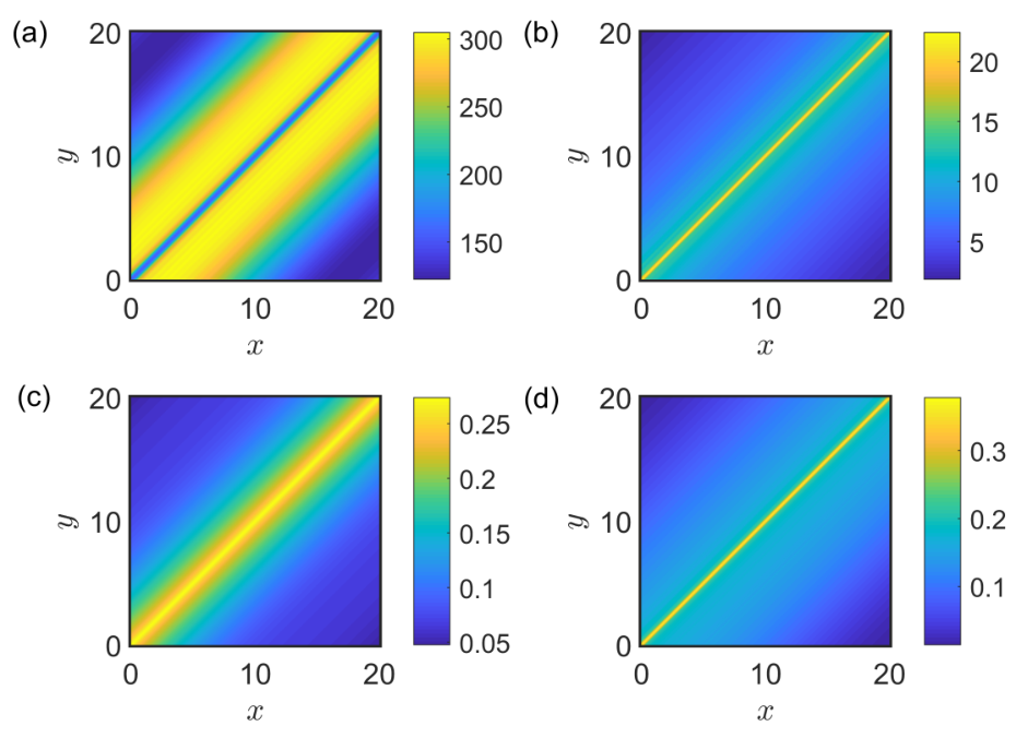
where and are the positions of two forward outgoing photons. indicates the correlation of detecting one photon at and the other photon at in the incoherent scattering process. Fig. S8 shows the correlation function of the outgoing photons when the total energies of incoming photon pairs match the first and second double-excited subradiant states. The parameters are chosen as , , , (a) , (b) , (c) and (d) , respectively. These parameters are corresponding to the four resonant peaks of the double-excited subradiant states in Fig. 3(a) and (b) of main text. When the double-excited subradiant states are excited, the forward outgoing photons show strong spatial correlations.
S4.4 D. Incoherent scattering in two and three qubits

The double-excited subradiant states are present for qubits. Thus, it is instructive to compare the incoherent scattering shown in Fig. 3 in the main text with the scattering in two and three qubits without any double-excited subradiant states, see Fig. S9. In the case of two qubits, there is only one single-excited subradiant state. The incoherent forward scattering is strongly enhanced when either of the individual incoming photons is resonant with the single-excited subradiant state, see the peaks along the dashed lines in Fig. S9(a)-(c), where the energy differences are fixed as for (a) and for (b), and other parameters are chosen as , . In Fig. S9(c), apart from the resonant peaks along the dashed line, there are also dark regions in scattering spectral along the line with . To better understand the dark regions, we calculate the incoherent scattering vs. and in Fig. S9(f), where the energy difference and . The incoherent scattering is normalized by the maximum value of the total incoherent forward scattering in a single qubit. The incoherent scattering is enhanced when and suppressed when . It is clear that the dip is lying at . When , the incoherent scattering is almost negligible due to the destructive quantum interference of two distinct excitation pathways Muthukrishnan et al. 2004. However, when increases (i.e. the atoms are not exactly at the same point), fully dark modes become subradiaint. As a result, more pathways start playing role in scattering and not all of these pathways interfere destructively. Thus, the incoherent scattering at the dip increases with . In Fig. S9(d) and (e), we show the incoherent scattering by fixing and , respectively. It is clear that the incoherent scattering in the dip of Fig. S9(e) is larger than that of Fig. S9(d).
We do the similar calculations for the case of qubits, where the parameters are chosen the same as the counterparts in the case of two qubits. Since there are single-excited subradiant states for three qubits, there are two resonant peaks in the incoherent scattering spectral where the energy of the individual incoming photons hits the single-excited subradiant states, see Fig. S9(g)-(i). When the total energy of the incoming photons are closed to , the incoherent scattering is also strongly suppressed due to the destructive interference, see Fig. S9(j)-(l). Similar to the case of two qubits, there are incoherent scattering can be enhanced only due to the single-excited subradiant states, and the incoherent scattering in the dip increases with .
As discussed in the main text, Fig. 3, for qubits double-excited subradiant states start playing role. They appear right in the dip with the resonant energy , and further enhance the incoherent scattering.
S5 S5. Threshold of qubit number for subradiant states
In the main text, we show that the double-excited subradiant state appears in the arrays with at least qubits. Generally, one may ask how many qubits support the appearance of excitation subradiant states. To reveal the threshold of the existence of subradiant state, we find the eigenstate with the energy around that has the minimal first-order decay rate. The decay rate of such state as excitation number and qubit number change is shown in Fig. S10. The calculation is based on the diagonalization of effective Hamiltonian, Eq. (2) of the main text, with the parameters and . The white region is unphysical for two-level qubits, since excitations cannot occupy the qubits. The threshold of subradiant state, determined as the moment when the decay rate drops down to , is denoted by the blue solid line. Thus, we can deduce that the threshold satisfies , in other words, the -excited subradiant states can be engineered only if the number of qubits exceeds .

S6 S6. Subradiant and twilight states in photon-photon correlations

In this section we demonstrate how the superradiant, subradiant and twilight states are manifested in the time-dependent photon-photon correlations. The wavefunction, describing the backscattering of the pair of photons, incident at the frequencies , is given by
| (S85) |
Here, the first term describes the coherent independent scattering of the photons, the second term accounts for the photon-photon correlations, and are the reflection coefficients for individual photons. We are interested in the time-dependent photon-photon correlations, that are given by
| (S86) | |||||
where . We consider the situation when the total energy of the photon pair is varied around , while the individual photon energies are strongly detuned from . This allows us to selectively and resonantly excite only the two-photon states. Due to the strong detuning between and , the first term in Eq. (S86) will rapidly oscillate in time. Hence, we assume that the time-dependent correlations are smoothed and defined in the following way:
| (S87) |
The normalization has been explicitly chosen to satisfy the condition . Since , in the regime when we obtain
| (S88) |
We note, that for due to the photon blockade effect [Poshakinskiy and Poddubny 2016]. The scattering amplitude , defined in Eq. (S71), depends on the energies of the scattered photons only via the single-particle Green functions, . As such, the lifetime of the correlations is determined only by the single-photon resonances. However, the excitation efficiency of the different single-photon resonances still does depend on the photon pair energy . This is the main ingredient of our proposal for observation of different two-photon states: when the pair energy is tuned to the double-excited subradiant or twilight state, the excitation efficiency of single-excited subradiant state increases, which results in long-lived photon-photon correlations.
In order to test this approach, we have plotted in Fig. S11 the dependence of the correlations on time and photon pair energy . The calculation demonstrates, that the spectra of the photon-photon correlations strongly depend on the delay time. Namely, at the spectrum is dominated by a broad feature with the half-width at half-maximum , corresponding to the excitation of the double-excited superradiant state [black curve in Fig. S11(b)]. However, the superradiant mode has short lifetime, and this broad feature is already vanished at . At larger time, , the spectrum becomes more narrow [red curve in Fig. S11(b)]. The narrow features with the width correspond to the excitation of the two-particle subradiant states. The wider features, with the width , are due to the twilight resonances.

The same contribution of the twilight states to the long-lived photon-photon correlations is also examined in Fig. S11c that shows the curves as function of time for different detunings . For large detunings ( and , blue and magenta curves) the correlations are practically independent of . As such, these long-lived traces are not related to the two-photon states. They are due to the subradiant single-particle resonances rather than double-excited states. However, the amplitude of long-lived photon-photon correlations in Fig. S11(c) is strongly modified when is tuned closer to (black and red curves). This is in full agreement with the results in Fig. S11(b) and is explained by the excitation of the twilight states.
Thus, the twilight states can be used for excitation of long-lived photon-photon correlations. They show the same long lifetime as the two-particle subradiant states, but are relatively easier to excite due to their broader spectral linewidth . The lifetime of photon-photon correlations is much longer than that of the individual qubits, see Fig. S12. In the case of single qubit, the photon-photon correlations quickly decay to with the decay rate , and they are almost independent of the average energy of incident photons. This means that the waveguide photons coupled to qubits arrays enable more potential applications in storage and processing of quantum information.
References
- Kashcheyevs and Kaestner (2010) V. Kashcheyevs and B. Kaestner, “Universal decay cascade model for dynamic quantum dot initialization,” Phys. Rev. Lett. 104, 186805 (2010).
- Muthukrishnan et al. (2004) A. Muthukrishnan, G. S. Agarwal, and M. O. Scully, “Inducing disallowed two-atom transitions with temporally entangled photons,” Phys. Rev. Lett. 93, 093002 (2004).
- Albrecht et al. (2019) A. Albrecht, L. Henriet, A. Asenjo-Garcia, P. B. Dieterle, O. Painter, and D. E. Chang, “Subradiant states of quantum bits coupled to a one-dimensional waveguide,” New J. Phys. 21, 025003 (2019).
- Zhang and Mølmer (2019) Y.-X. Zhang and K. Mølmer, “Theory of subradiant states of a one-dimensional two-level atom chain,” Phys. Rev. Lett. 122, 203605 (2019).
- Zhang et al. (2019) Y.-X. Zhang, C. Yu, and K. Mølmer, “Subradiant dimer excited states of atom chains coupled to a 1D waveguide,” arXiv:1908.01818 (2019).
- Poshakinskiy and Poddubny (2016) A. V. Poshakinskiy and A. N. Poddubny, “Biexciton-mediated superradiant photon blockade,” Phys. Rev. A 93, 033856 (2016).
apsrev41Control