Conformally symmetric traversable wormholes in gravity
Abstract
To find more deliberate astrophysical solutions, we proceed by studying wormhole geometries under the assumption of spherical symmetry and the existence of a conformal Killing symmetry to attain the more acceptable astrophysical results. To do this, we consider a more plausible and simple model , where is the Ricci scalar and denotes the trace of the energy-momentum tensor of the matter content. We explore and analyze two cases separately. In the first part, wormhole solutions are constructed for the matter sources with isotropic pressure. However, the obtained solution does not satisfy the required wormhole conditions. In the second part, we introduce an EoS relating to pressure (radial and lateral) and density. We constrain the models with phantom energy EoS i.e. , consequently violating the null energy condition. Next, we analyze the model via . Several physical properties and characteristics of these solutions are investigated which are consistent with previous references about wormholes. We mainly focus on energy conditions (NEC, WEC and SEC) and consequently for supporting the respective wormhole geometries in details. In both cases it is found that the energy density is positive as seen by any static observer. To support the theoretical results, we also plotted several figures for different parameter values of the model that helps us to confirm the predictions. Finally, the volume integral quantifier, which provides useful information about the total amount of exotic matter required to maintain a traversable wormhole is discussed briefly.
Keywords:
gravity; CKV; Wormhole Solutionpacs
04.20.Gz, 11.27.+d, 04.62.+v, 04.20.−qI Introduction
Traversable Lorentzian wormholes are hypothetical tunnels in space-time that connects two regions of the same or disjointed universes. These problems can be attributed in classical general relativityو in which observers may freely traverse. Since wormhole has a long history, but it was developed mainly with the seminal paper by Morris and Thorne Morris, in 1988 as a toy model allowing for interstellar travel. In particular, these geometries have a minimal surface area linked to satisfy flare-out condition, which is called throat of the wormhole. A stress-energy tensor that violates the null energy condition is involving to grip such a wormhole open Visser. Roughly speaking, the matter that violates the weak/null energy conditions called ‘exotic matter’. Such strange objects exists both in the static Anabalon:2012tu; Balakin:2010ar; Jamil:2009vn; Cataldo:2002jw and dynamic Dehghani:2009xu; Bochicchio:2010df; DeBenedictis:2008qm; GonzalezDiaz:2003pb; Cataldo:2011zn; Hansen:2009kn cases, and sustained by a single fluid component. The violation of the energy conditions have been supported by many arguments like the quantum field theories such as the Casimir effect, Hawking evaporation and scalar-tensor theories. Though the usage of exotic matter is a problematic issue. Visser et al. Visser:2003yf have proposed ‘volume integral quantifier’ that how to quantify the total average null energy conditions for wormhole maintenance.
However, a static wormhole without violating the energy conditions in the framework of Einstein General Relativity is still an open problem, which can be motivated to minimize the usage of exotic matter by applying the cut and paste technique, which was proposed by Visser Visser:1989kh; Visser:1989kg. The proposal was to restrict the exotic fluid at the wormhole throat. There were another solution came from Kuhfittig Kuhfittig:2002ur; Kuhfittig:1999ur to hamper the exotic fluid of an arbitrary thin region by imposing a condition on to be close to one at the throat.
One may also follow a more conventional method to address the issue in an alternatives theories of gravity. The physical incentives for these amendments of gravity are based on gravitational actions which are linked to the possibility of a more realistic illustration of the gravitational fields near curvature singularities. The main purpose of this approach lies on the assumption that matter threading the wormhole satisfies the energy conditions. Due to the effective stress-energy tensor, the field equations have to rewritten in a form that represented as a sum of the standard fluid plus the new terms coming from the modified theory. In this context, several wormhole solutions were analyzed in various modified gravity theories such as gravity Lobo:2009ip; DeBenedictis:2012qz; Mazharimousavi:2012xv; DiCriscienzo:2013ria; Eiroa:2015hrt; Pavlovic:2014gba, gravity wormhole with noncommutative geometry Jamil:2013tva, gravity Sharif:2013exa; Sharif:2014bsa; Sharif:2013lya, noncommutative geometry Rahaman:2012pg; Zubair:2019qqz; bhar2014, Lovelock solutions Dehghani:2009zza; Matulich:2011ct; Zangeneh:2015jda; Mehdizadeh:2016nna and in others.
In this article, we are particularly interested in gravity Harko:2011kv, where the Lagrangian is an arbitrary function of Ricci scalar and the trace of the energy-momentum tensor . This theory has been tested from cosmology to astrophysics and are more manageable compared to theories. Recently, this model has been extensively investigated, such as thermodynamics properties frttd1; frttd2; frttd3, energy conditions frtec1; frtec2; frtec3, cosmological solutions based on a homogeneous and isotropic space–time through a phase–space analysis phsp, a cosmological solution via a reconstruction program frtrec1; frtrec2, anisotropic cosmology frtani2; frtani3, a cosmological solution via an auxiliary scalar field frtaf, the study of scalar perturbations frtsp. But, a serious shortcoming in this modification has been the non-conservation of the energy-momentum tensor. Non-conservation of the energy-momentum tensor is also found in relativistic diffusion models (Ref. Calogero and references therein). This fact has to be stressed because it demonstrates somehow a limitation for this class of theories. However, consistent cosmological solutions are in favor of this theory. For detailed review of - gravity one may refer to Houndjo:2011fb. In the following, a static wormhole solution have been obtained by Moraes & Sahoo Moraes:2017mir. Also, a charged wormholes in gravity has been proposed recently in Moraes:2017rrv; Banerjee:2020uyi.
The theoretical construction of wormhole geometries lies on the fact that one has a desired metric, which have to solve by fixing the form of the metric potential functions or by using a precise equation of state that relates the pressure with the energy density, and then solve Einstein’s field equations. In our work an exact solutions by assuming spherical symmetry and the existence of a non-static conformal symmetry have been studied in an alignment of systematic approach that was considered previously by Boehmer et al Boehmer:2007rm; Boehmer:2007md. The study of conformal symmetry gives a natural link between geometry and matter through the Einstein field equations. It is for this reason the vector has been specified as the generator of this conformal symmetry, then the metric is conformally mapped onto itself along , which is interpreted into the following relationship
| (1) |
where is the Lie derivative operator of the metric tensor and is the conformal killing vector. Also, for a static metric, we have noted that neither nor need to be static. This approach was used in Herrera1984; Herrera1985, to show that for a one-parameter group of conformal motions, the EoS is uniquely determined by the Einstein equations. Later, this particular exact solution was extended by Maartens & Maharaj Maartens, for static spheres of charged imperfect fluids with assuming space-time admits a conformal symmetry. Very recently, Kuhfittig Kuhfittig:2016pyx; Kuhfittig:2015cea have studied wormholes admitting a one-parameter group of conformal motions.
The plan of this paper is as follows: After the introduction in Section I, we briefly
review the field equations of gravity, in particular when the matter is minimally coupled to the curvature in a specific form, are presented in Section II.
In Section III, we discuss a specific spacetime metric (Morris-Thorne metric) of a spherically symmetric traversable wormhole and the basic mathematical criteria.
In Section IV, exact general solutions are deduced using static conformal symmetries. In section V, we present the unique exterior vacuum solution.
Then, we study the wormhole models from different hypothesis for their matter content; specifically for isotropic pressure and linear EoS relating the energy density and the pressure anisotropy in section VI. Finally, in Section VII, we conclude.
II Basic mathematical formalism of the Theory
In this section, we start by writing the general action for modified gravity in four-dimensional spacetime. The full action is given by Harko et al Harko:2011kv (with geometrized units )
| (2) |
where is an arbitrary function depends on a generic function of and , the Ricci scalar and the trace of the energy momentum tensor , respectively. From the matter Lagrangian density , we defined the energy-momentum tensor as follows
| (3) |
Following the argument in Harko:2011kv, we assume that the Lagrangian density depends only on the metric components and not on its derivatives, we obtain
| (4) |
Now, by variation of the action given in Eq. (2) with respect to the metric , to obtain the gravitational field equation for gravity as:
| (5) |
where , , , is the Ricci tensor, denotes the covariant derivative with respect to the metric and .
Performing a covariant divergence of (5) which yield Baffou:2013dpa; Singh:2013bpa; Sharif:2014ioa; Baffou:2017pao; Mishra_2018
| (6) |
For this purpose we assume the matter content of the wormhole solution is an anisotropic fluid and one can write the energy momentum tensor as
| (7) |
where is the energy density with and representing the radial and tangential pressures of the fluid, is the four-velocity such that and . In this way, one can choose the matter Lagrangian density as , where which is more generic, in the sense that they do not imply the vanishing of the extra force, which yields .
In the present work, we focus our attention on the simplified and linear functional form of , as suggested by Harko et al Harko:2011kv, where is a constant. The chosen form has been broadly applied in many cosmological solutions of gravity Houndjo:2011fb. Our ansatz for the function , the Eq. (5) becomes Moraes:2017mir; Moraes:2017rrv
| (8) |
where is the Einstein tensor. If we set , then one can easily recover the general relativistic result. It is straightforward to see that for the particular choice of , Eq. (4) leads to the form
| (9) |
Regarding the Bianchi identity, obviously in gravity, the covariant derivative of the energy-momentum tensor is not null in general. But substituting in Eq. (9), one can see that the energy-momentum tensor is conserved as in case of general relativity.
III Traversability conditions and general remarks for wormholes
The spacetime ansatz for seeking traversable static spherically symmetric wormholes is the Morris-Thorne metric Morris, which can be written as
| (10) |
where and are the redshift and the shape functions, respectively. The redshift function must be finite everywhere, in order to ensure the absence of horizons and singularities. The essential characteristics of a wormhole is the shape function which determine the shape of the wormhole must satisfy the condition ) = at the throat where . For the existence of standard wormholes, the shape function should satisfy the “flaring-out condition”, given by
| (11) |
which reduces to at the throat . Here the prime denotes the derivative with respect to the radial coordinate . Moreover, finiteness of the proper radial distance, defined by
| (12) |
is required to be finite everywhere. It is important to note that ‘’ the proper distance is greater than or equal to the coordinate distance, i.e. where the signs refer to the two asymptotically flat regions which are connected by the wormhole. Since, decreases from to at the throat of the wormhole , and then from to .
Following the metric Eq. (10), the Einstein tensor, = then reduce to the following non-zero components
| (13) | |||||
| (14) | |||||
| (15) | |||||
| (16) |
where primes stand for derivation with respect to the radial coordinate .
IV The Conformal Killing Vector (CKV)
Construction of wormhole can be straightforwardly generalised to conformal theories containing matter fields. Based on the assumption that spherically symmetric static space-time possesses a conformal symmetry and identify its essential mathematical structure, one can simplify the treatment of the problem and define its basic mathematical structure Herrera1984; Maartens. The existence of a Killing vector laid constraints on the influences of curvatures of the manifold and symmetry. If we consider a static metric, the vector fields and are not necessary to be static. So, the Eq. (1) can be written in a simple way as
| (17) |
where the Lie derivative operators and describes the interior gravitational field of a wormhole configuration. Constants of the motion may be determined by the Killing vectors i.e. quantities that will be constant along any given geodesic. Furthermore, the conformal vectors can be obtained when (i) , then Eq. (17) gives the Killing vector, (ii) constant gives homothetic vector, and (iii) when gives conformal vectors.
After introducing conformal Killing vector Eq. (17) into the metric Eq. (10), without a loss of generality provides the following solutions
where and represents the spatial and temporal coordinates and , respectively.
These, in turn, imply that
| (18) | |||||
| (19) | |||||
| (20) |
where , and are constants of integration. Notice that if the Eq. (19) written in terms of the shape function , then the conformal factor is zero at the throat, i.e. . It should be emphasized that the solutions given by Eqs. (18) and (19), and using the above conformal relations relating the form and redshift functions places a strong constraint on the specific choices of the wormhole geometries. From the above relation, it is obvious that imposing the choices for the redshift function, one may deduce the form function and the conformal factor also.
The strong constraints on the wormhole geometry will be imposed by the existence of conformal motions. Consider the above energy-momentum tensor and the Morris-Thorne metric Eq. (10), the generalized gravitational field equations (8) give the following field equations
| (21) | |||
| (22) | |||
| (23) |

Thus, using the expression (18)-(20), in the above Eqs. (21)-(23), we obtain a set of field equations as follows
| (24) | |||||
| (25) | |||||
| (26) |
where the and are given by
In addition to other essential characteristics of a wormhole solution, the violation of the null energy condition (NEC) at the throat of the wormhole is a generic feature. Therefore, such energy conditions are deemed important since they lead to physical requirements on matter.
Considering the gravity, Garcia and Lobo MontelongoGarcia:2010xd showed that nonminimal coupling minimizes the violation of the NEC of normal matter at the throat. Moreover, Einstein-Cartan theory attracted a good deal of attention in wormhole solution without invoking exotic matter Bronnikov:2015pha. Quantum effects also produce violations of the classical energy conditions, amongst which the popular one is Casimir effect.
In the context of the local energy conditions, we examine the the violation of NEC, , where is any null vector and is the usual Hilbert stress-energy-momentum tensor. In combination to the above expression we have
| (27) |
which evaluated at the throat imposes the following condition (.

V Thin shell around traversable wormhole
We shall model specific static wormholes by matching an interior geometry, with an exterior Schwarzschild vacuum solution, at a junction interface = . Our aim here is to restrict the dimensions of these wormholes not to arbitrarily large. For this, the exterior Schwarzschild is given by
| (28) |
which we shall match with the interior spacetime given in Eq. (10).
Following the standard junction-condition formalism in (3 +1)-dimensional spacetime Musgrave:1995ka; Sen:1924; Lanczos:1924; Israel:1967, one can consider two pseudo-Riemannian manifolds with a radius greater than the event horizon radius, and paste them at the hypersurface to create a geodesically complete manifold. If such boundaries are identified, then a natural match of manifolds can be done, with two regions connected by a throat of radius, where the exotic matter is located Poisson:1995sv; Bejarano:2006uj; Eiroa:2003wp; Lemos:2008aj; Rahaman:2008xs; Forghani:2018gza; Banerjee:2016blr; Banerjee:2012aja. Beyond GR, the junction formalism requires to be generalized and several conditions that should be fulfilled for the specific theory of gravity under consideration. For example in gravity, the junction conditions tend not to always coincide with those of general relativity Deruelle:2007pt; Senovilla:2013vra; Goswami:2014lxa (see also Refs. Velay-Vitow:2017odc for gravity).
To understand the above in some details we would like to point out a special feature of the thin-shell structure. More tactically for a geodesically complete thin-shell wormholes, the Riemann tensor is divergent at the thin-shell where the throat is located Poisson. To see this let be a non-null hypersurface layer, and suppose the coordinate system on both sides of the hypersurface to be the same then defines the jump of a quantity as
| (29) |
Then, the distribution of matter reads
| (30) |
so that the geodesics cross when , and . For further details, we refer the reader to Bejarano:2016gyv. The quantity is known as the Heaviside step function whereas is the surface stress-energy tensor on the thin-shell.
It is interesting that this way the curvature of spacetime becomes divergent at for thin-shell wormholes (because the Riemann tensor is singular). But this divergence is physically interpreted as a surface layer with a stress-energy tensor on it. Therefore, the existence of curvature divergences exists at the wormhole throat.

VI Conformal Symmetry Wormhole
In general, to solve the three field equations Eqs. (24-26) with the following four unknown functions of , namely, , , and is mathematically well-defined problem. For obtaining an explicit solution one has to specify or determine the EoS, the shape function etc. by implementing some physical conditions. We employ the following approach to extract and analyze the solutions as below.
VI.1 On spherical wormhole with isotropic pressure
The case of a isotropic wormhole i.e. when is particularly simple one, yet it provides enough interesting results Cataldo:2016dxq. In order to analyze solutions we shall now on take into consideration Eqs. (24) and (25), which yield
| (31) |
where the constant term is determined by imposing the condition at the throat of the wormhole. Now, using the condition in Eq. (19), we obtain the form of shape function as
| (32) |
The aim of this section is to see the behavioral effects of and its derivative . Here the throat of wormhole is located at . From the obtained shape function (32), one can easily check that .
In principle, flaring-out condition at the throat should obey the following inequality , which is not reflecting for isotropic pressure wormhole solution.
VI.2 Wormhole solutions with specific choices
In the following analysis, we consider the relationship involving specific form of equation of state and anisotropy to solve the field equations.
VI.2.1 WH1: Model with
With the definitions of and , one can rewrite the field equations (24)-(26) further in the following form:
| (33) | |||||
| (34) | |||||
| (35) |
Let us start for searching an exact wormhole model by considering a linear EoS which is characterized by . Now, if we take account of (33) and (34) then, after integration, we can recover the functional form of , which yield
| (36) | |||||
and the corresponding shape function takes the form
| (37) | |||||
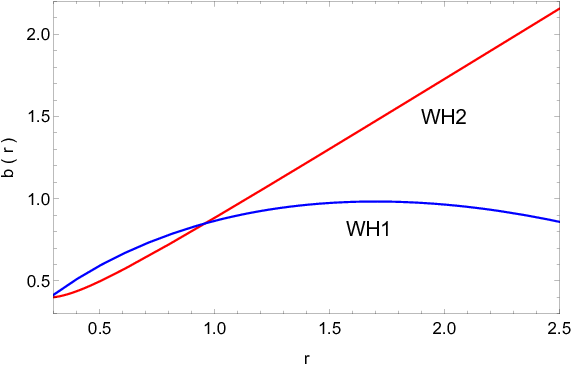
In this case we have for the metric component if . In Fig. (1), we show the behavior of shape function for . This result shows that a wormhole solution requires a phantom-energy background, i.e. . The use of phantom-energy is not new in wormhole physics (see refs. Zaslavskii:2005fs; Cataldo:2008ku; Jamil:2008wu; Lobo:2012qq; Nandi:2016ccg). The energy density in cosmology setting related to the phantom energy is considered positive, , and we shall maintain this condition.
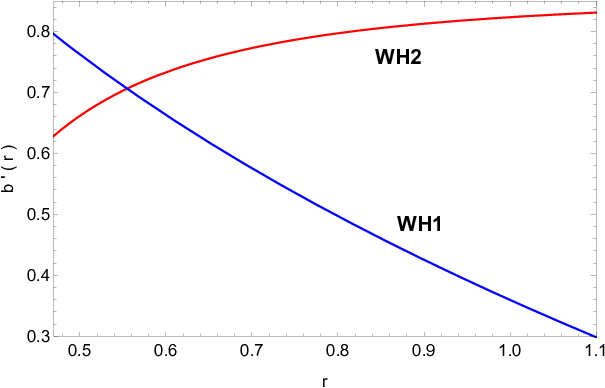
The graphical behavior of the , , and are depicted in Figs. 2-4 for WH1 and WH2. From Fig. 3, we find that cuts the -axis, with the throat at = 0.757 and 5.1, respectively. We also observe that , which obeys the flaring out condition appear in Fig. 4. Moreover, we can see directly from Fig. 2 that the asymptotic behavior as , but the redshift function does not approach zero as , which is expected for conformally symmetric wormhole Rahaman:2014dpa; Bhar:2016vdn. This means the wormhole spacetime is not asymptotically flat, so one needs to match these interior geometries to an exterior vacuum spacetime, at a junction interface which we have discussed in sec V.
Thus, in this case the stress-energy tensor components are given by
| (38) | |||||
| (39) | |||||
| (40) | |||||
To see in a more quantitative way we also analyzed the energy conditions. In Fig. 5, we present the graphical behavior of the NEC, WEC and the SEC in terms of the , and , for different values of parameters , and . Fig. 5, shows the validity of (blue). With the above solution we also found that but that ensure the violation of NEC and this lead to the violation of WEC also. One can see from figure that the SEC (brown) is also violated.
Now, we can construct embedding diagrams to represent a wormhole and extract some useful information for the obtained shape function, .
Considering a fixed moment of time, & and embed the metric into three-dimensional Euclidean space, we obtain the embedding surface which is given by
| (41) |
For this particular case, the above equation becomes
| (42) |

which on integration, we get
| (43) | |||||
where
The embedded surface and surface of the revolution for about the axis are shown in Figs. 7 and 8.


VI.2.2 WH2: Model with
Here, we investigate the wormhole solution for a particularly interesting anisotropy, already explored in Rahaman:2006xa; Moraes:2017mir, given by
| (44) |
where the state parameter is a constant. With this assumption and solving the differential equations (33)-(35), as the same procedure for WH1, the function takes the form
| (45) | |||||
where and .
Using the definition of provided in Eq. (19), one can find the shape function as
As we can see from Fig. 2, that the solutions are asymptotically flat, i.e. as , because of decreasing graphs with increasing . In addition, we plot in Figs. 3 and 4, the characteristic picture of the shape function. The red curve represents a regular wormhole solution which cuts -axis at 0.494 is the throat of the WH2. As seen in the figure 4, that , which obeys the flaring out condition. Clearly, in this case also for , the redshift function does not approach zero. Thus, one needs to match this solution to an exterior spacetime at a junction interface, .
Now, the stress-energy tensor components for the EoS are given by
| (47) | |||||
| (49) |
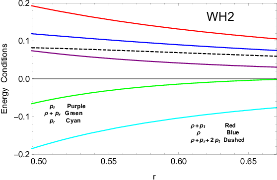
To determine the energy conditions we have plotted graphs, and Fig. 6 illustrates the behaviour of the null, weak and strong energy conditions. Clearly, in this case we have (blue curve). We are mostly interested in the NEC, because its violation implies the violation of WEC also. In Fig. 6, but i.e. violation of NEC and consequently the WEC, are violated. Interestingly we note that SEC (dashed curve) is satisfied in this case. All solutions are characterized by considering parameter values and for WH2.
VII Volume integral quantifier
It is convenient to consider the “volume integral quantifier” to know how much of exotic matter is required to support a traversable Lorentzian wormhole on a local scale. This was first prompted by Visser et al Visser:2003yf. Later, a more technical review was proposed in Nandi:2004ku. Quantifying the amount of exotic matter has been considered by the following defined integral , and with a cut-off of the stress-energy at is given by
| (51) | |||||
where , and the boundary term at vanishes by our construction as . Then, the volume-integral reduce to (see Ref. Boehmer:2007md for more details)
| (52) | |||||
Taking into account the redshift function , and the form function, Eqs. (37) and (VI.2.2), we obtain the following expression
| (53) | |||||
| (54) | |||||
where . It is interesting to note that when then for both cases. In fact, one can also observe that for WH1 if the parameter arbitrary close to , the integral may be infinitesimally small. These results fundamentally confirm the validity of conformally symmetric phantom wormhole solutions, as described in Lobo:2005us; Lobo:2005yv, where the violation of ANEC is arbitrarily small when the interior solution is matched to an exterior vacuum spacetime.
VIII SUMMARY AND DISCUSSION
In the present paper, we investigate the possible existence of wormhole solutions in the framework of gravity under the assumption of spherical symmetry and the existence of a conformal Killing symmetry. To address the problem we consider a particular and simple model , where is the Ricci scalar and denotes the trace of the energy–momentum tensor of the matter content. Even within this simple theoretical model the field equations become extremely complicated, and therefore conformal symmetry is a more systematic approach in searching for exact analytic solution. The obtained solutions in this article are not asymptotically flat, where distribution of the exotic matter restricted to the throat neighborhood, and we consider a cut-off of the stress-energy tensor at a junction interface by matching an interior traversable wormhole geometry. In fact, we are successfully able to make the a particular asymptotically flat wormhole geometries where the dimensions are not arbitrarily large.
Next, we explore and analyze two cases separately. At the first part, the obtained wormhole solutions are constructed for the matter sources with isotropic pressure. However, showing explicitly that the solution violates the basic criteria for wormhole. Further, we proceed by introducing an EoS relating with pressure (radial and lateral) and density. We show the possibility of having traversable wormhole geometries supported by phantom energy. In this case, the energy density is positive which consequently violates the null energy condition. However, we emphasize that when the volume integral quantifier would by itself become arbitrarily small i.e. theoretically it is possible to construct these geometries with vanishing amounts of ANEC. For our convenience we have also analyzed physical properties and characteristics of traversable wormholes by using graphical representation (see Fig. 1-8).
In the second part of the paper we obtain a similar picture for the models described by . Still in this case, obtained solution are violating the NEC and WEC with the energy density , but interestingly satisfying the SEC. From our analysis it is very transparent that the assumption of a static conformal symmetry, i.e., with a static vector , is found responsible to find an exact solutions of traversable wormholes.
Acknowledgments
FR would like to thank the authorities of the Inter-University Centre for Astronomy and Astrophysics, Pune, India for providing the research facilities. FR is also thankful to DST-SERB, Govt. of India and RUSA 2.0, Jadavpur University, for financial support.
References
- (1) M.S. Morris and K.S. Thorne: Am. J. Phys., 56, 395 (1988).
- (2) M. Visser, Lorentzian Wormholes: From Einstein to Hawking (American Institute of Physics, New York, 1995).
- (3) A. Anabalon and A. Cisterna, Phys. Rev. D 85, 084035 (2012).
- (4) A. B. Balakin, J. P. S. Lemos and A. E. Zayats, Phys. Rev. D 81, 084015 (2010).
- (5) M. Jamil, P. K. F. Kuhfittig, F. Rahaman and S. A. Rakib, Eur. Phys. J. C 67, 513 (2010).
- (6) M. Cataldo, P. Salgado and P. Minning, Phys. Rev. D 66, 124008 (2002).
- (7) M. H. Dehghani and S. H. Hendi, Gen. Rel. Grav. 41, 1853 (2009).
- (8) I. Bochicchio and V. Faraoni, Phys. Rev. D 82, 044040 (2010).
- (9) A. DeBenedictis, R. Garattini and F. S. N. Lobo, Phys. Rev. D 78, 104003 (2008).
- (10) P. F. Gonzalez-Diaz, Phys. Rev. D 68, 084016 (2003).
- (11) M. Cataldo, P. Meza and P. Minning, Phys. Rev. D 83, 044050 (2011).
- (12) J. Hansen, D. I. Hwang and D. h. Yeom, JHEP 0911, 016 (2009).
- (13) M. Visser, S. Kar and N. Dadhich, Phys. Rev. Lett. 90, 201102 (2003).
- (14) M. Visser, Phys. Rev. D 39, 3182 (1989).
- (15) M. Visser, Nucl. Phys. B 328, 203 (1989).
- (16) P. K. F. Kuhfittig, Phys. Rev. D 66, 024015 (2002).
- (17) P. K. F. Kuhfittig, Am. J. Phys. 67, 125 (1999).
- (18) F. S. N. Lobo and M. A. Oliveira, Phys. Rev. D 80, 104012 (2009).
- (19) A. DeBenedictis and D. Horvat, Gen. Rel. Grav. 44, 2711 (2012).
- (20) S. Habib Mazharimousavi and M. Halilsoy, Mod. Phys. Lett. A 31, 1650203 (2016).
- (21) R. Di Criscienzo, R. Myrzakulov and L. Sebastiani, Class. Quant. Grav. 30, 235013 (2013).
- (22) E. F. Eiroa and G. Figueroa Aguirre, Eur. Phys. J. C 76, 132 (2016).
- (23) P. Pavlovic and M. Sossich, Eur. Phys. J. C 75, 117 (2015).
- (24) M. Jamil, F. Rahaman, R. Myrzakulov, P. K. F. Kuhfittig, N. Ahmed and U. F. Mondal, J. Korean Phys. Soc. 65, 917 (2014).
- (25) M. Sharif and S. Rani, Phys. Rev. D 88, 123501 (2013).
- (26) M. Sharif and S. Rani, Adv. High Energy Phys. 2014, 691497 (2014).
- (27) M. Sharif and S. Rani, Gen. Rel. Grav. 45, 2389 (2013).
- (28) F. Rahaman, S. Islam, P. K. F. Kuhfittig and S. Ray, Phys. Rev. D 86, 106010 (2012).
- (29) M. Zubair, S. Waheed, G. Mustafa and H. Ur Rehman, Int. J. Mod. Phys. D 28, 1950067 (2019).
- (30) P. Bhar and F. Rahaman, Eur. Phys. J. C 74, 3213 (2014).
- (31) M. H. Dehghani and Z. Dayyani, Phys. Rev. D 79, 064010 (2009).
- (32) J. Matulich and R. Troncoso, JHEP 1110, 118 (2011).
- (33) M. Kord Zangeneh, F. S. N. Lobo and M. H. Dehghani, Phys. Rev. D 92, 124049 (2015).
- (34) M. R. Mehdizadeh and F. S. N. Lobo, Phys. Rev. D 93, 124014 (2016).
- (35) T. Harko, F. S. N. Lobo, S. Nojiri and S. D. Odintsov, Phys. Rev. D 84, 024020 (2011).
- (36) M. J. S. Houndjo, F. G. Alvarenga, M. E. Rodrigues and D. F. Jardim, Eur. Phys. J. Plus 129, 171 (2014).
- (37) M. Sharif and M. Zubair, J. Cosmol. Astropart. Phys. 03, 028 (2012).
- (38) M. Jamil, D. Momeni and M. Ratbay, Chin. Phys. Lett. 29, 109801 (2012).
- (39) F.G. Alvarenga, M.J.S. Houndjo, A.V. Monwanou and J.B. Chabi Orou, J. Mod. Phys. 04, 130 (2013).
- (40) M. Sharif and M. Zubair, J. High Energy Phys. 12, 079 (2013).
- (41) F. Kiani and K. Nozari, Phys. Lett. B 728, 554 (2014).
- (42) H. Shabani and M. Farhoudi, Phys. Rev. D 88, 044048 (2013).
- (43) M. Jamil, D. Momeni, M. Raza and R. Myrzakulov, Eur. Phys. J. C 72, 1999 (2012).
- (44) M. Sharif and M. Zubair, Astrophys. Space Sci. 349, 529 (2014).
- (45) M. Kiran and D. R. K. Reddy, Astrophys. Space Sci. 346, 521 (2013).
- (46) M. Sharif and M. Zubair, Astrophys. Space Sci. 349, 457 (2014).
- (47) M. J. S. Houndjo, Int. J. Mod. Phys. D 21, 1250003 (2012).
- (48) F.G. Alvarenga, A. Cruz–Dombriz, M. J. S. Houndjo, M. E. Rodrigues and D. Sáez–Gómez, Phys. Rev. D 87 (2013), 103526.
- (49) S. Calogero and H. Velten, J. Cosmol. Astropart. Phys. 11 025 (2013).
- (50) M. J. S. Houndjo and O. F. Piattella, Int. J. Mod. Phys. D 21, 1250024 (2012).
- (51) P. H. R. S. Moraes and P. K. Sahoo, Phys. Rev. D 96, 044038 (2017).
- (52) P. H. R. S. Moraes, W. de Paula and R. A. C. Correa, Int. J. Mod. Phys. D 28, 1950098 (2019).
- (53) A. Banerjee, M. K. Jasim and S. G. Ghosh, arXiv:2003.01545 [gr-qc].
- (54) C. G. Boehmer, T. Harko and F. S. N. Lobo, Phys. Rev. D 76, 084014 (2007).
- (55) C. G. Boehmer, T. Harko and F. S. N. Lobo, Class. Quant. Grav. 25, 075016 (2008).
- (56) L. Herrera et al, J. Math. Phys. 25, 3274 (1984);
- (57) L. Herrera and J. Ponce de Leon, J. Math. Phys. 26, 2303 (1985).
- (58) R. Maartens and M. S. Maharaj, J. Math. Phys. 31, 151 (1990).
- (59) P. K. F. Kuhfittig, Int. J. Mod. Phys. D 26, 1750025 (2016).
- (60) P. K. F. Kuhfittig, Annals Phys. 355, 115 (2015).
- (61) E. H. Baffou, A. V. Kpadonou, M. E. Rodrigues, M. J. S. Houndjo and J. Tossa, Astrophys. Space Sci. 356, 173 (2015).
- (62) C. P. Singh and V. Singh, Gen. Rel. Grav. 46, 1696 (2014).
- (63) M. Sharif and M. Zubair, Gen. Rel. Grav. 46, 1723 (2014).
- (64) E. H. Baffou, M. J. S. Houndjo, M. Hamani-Daouda and F. G. Alvarenga, Eur. Phys. J. C 77, 708 (2017).
- (65) B. Mishra, S. Tarai and S. K. Tripathy, Mod. Phys. Lett. A 33, 1850170 (2018).
- (66) N. Montelongo Garcia and F. S. N. Lobo, Class. Quant. Grav. 28, 085018 (2011).
- (67) K. A. Bronnikov and A. M. Galiakhmetov, Grav. Cosmol. 21, 283 (2015).
- (68) P. Musgrave and K. Lake, Class. Quant. Grav. 13, 1885 (1996).
- (69) N. Sen, Ann. Phys. (Leipzig) 73, 365 (1924).
- (70) K. Lanczos, Ann. Phys. (Leipzig) 74, 518 (1924).
- (71) W. Israel, Nuovo Cimento 44B, 1 (1966); 48B, 463(E) (1967).
- (72) E. Poisson and M. Visser, Phys. Rev. D 52, 7318 (1995).
- (73) C. Bejarano, E. F. Eiroa and C. Simeone, Phys. Rev. D 75, 027501 (2007).
- (74) E. F. Eiroa and G. E. Romero, Gen. Rel. Grav. 36, 651 (2004).
- (75) J. P. S. Lemos and F. S. N. Lobo, Phys. Rev. D 78, 044030 (2008).
- (76) F. Rahaman, M. Kalam and K. A. Rahman, Mod. Phys. Lett. A 24, 53 (2009).
- (77) S. D. Forghani, S. Habib Mazharimousavi and M. Halilsoy, Eur. Phys. J. C 78, 469 (2018).
- (78) A. Banerjee, K. Jusufi and S. Bahamonde, Grav. Cosmol. 24, 71 (2018).
- (79) A. Banerjee, F. Rahaman, S. Chattopadhyay and S. Banerjee, Int. J. Theor. Phys. 52, 3188 (2013).
- (80) N. Deruelle, M. Sasaki and Y. Sendouda, Prog. Theor. Phys. 119, 237 (2008).
- (81) J. M. M. Senovilla, Phys. Rev. D 88, 064015 (2013).
- (82) R. Goswami, A. M. Nzioki, S. D. Maharaj and S. G. Ghosh, Phys. Rev. D 90, 084011 (2014).
- (83) J. Velay-Vitow and A. DeBenedictis, Phys. Rev. D 96, 024055 (2017).
- (84) E. Poisson, A Relativist’s Toolkit: The Mathematics of Black-Hole Mechanics (Cambridge University Press, New York, 2004).
- (85) C. Bejarano, F. S. N. Lobo, G. J. Olmo and D. Rubiera-Garcia, Eur. Phys. J. C 77, 776 (2017).
- (86) M. Cataldo, L. Liempi and P. Rodríguez, Phys. Lett. B 757, 130 (2016).
- (87) O. B. Zaslavskii, Phys. Rev. D 72, 061303 (2005).
- (88) M. Cataldo, S. del Campo, P. Minning and P. Salgado, Phys. Rev. D 79, 024005 (2009).
- (89) M. Jamil, U. Farooq and M. A. Rashid, Eur. Phys. J. C 59, 907 (2009).
- (90) F. S. N. Lobo, F. Parsaei and N. Riazi, Phys. Rev. D 87, 084030 (2013).
- (91) K. K. Nandi, A. A. Potapov, R. N. Izmailov, A. Tamang and J. C. Evans, Phys. Rev. D 93, 104044 (2016).
- (92) F. Rahaman, I. Karar, S. Karmakar and S. Ray, Phys. Lett. B 746, 73 (2015).
- (93) P. Bhar, F. Rahaman, T. Manna and A. Banerjee, Eur. Phys. J. C 76, 708 (2016).
- (94) F. Rahaman, M. Kalam, M. Sarker, A. Ghosh and B. Raychaudhuri, Gen. Rel. Grav. 39, 145 (2007).
- (95) K. K. Nandi, Y. Z. Zhang and K. B. Vijaya Kumar, Phys. Rev. D 70, 127503 (2004).
- (96) F. S. N. Lobo, Phys. Rev. D 71, 084011 (2005).
- (97) F. S. N. Lobo, Phys. Rev. D 71, 124022 (2005).