跳到论文正文
W Papers独立论文阅读器 arXiv:1908.04540 论文正文 计算阅读时间 · 0%
引用这篇论文根据当前论文元数据生成,正式投稿前建议核对。


License: arXiv.org perpetual non-exclusive license
arXiv:1908.04540v2 [math.CA] 10 Apr 2020

Differential Equations for the Recurrence Coefficients Limits for Multiple Orthogonal Polynomials from a Nevai Class

Alexander I. Aptekarev1 ${}^{1}$Keldysh Institute of Applied Mathematics,
Russian Academy of Science,
Miusskaya Pl.4, Moscow 125047, Russian Federation; e-mail: aptekaa@keldysh.ru
and Rostyslav Kozhan2 ${}^{2}$Uppsala University
Box 480, 751 06 Uppsala, Sweden; e-mail: kozhan@math.uu.se
Date: August 11, 2026
Abstract.

A limiting property of the nearest-neighbor recurrence coefficients for multiple orthogonal polynomials from a Nevai class is investigated. Namely, assuming that the nearest-neighbor coefficients have a limit along rays of the lattice, we describe it in terms of the solution of a system of partial differential equations.

In the case of two orthogonality measures the differential equation becomes ordinary. For Angelesco systems, the result is illustrated numerically.

Key words and phrases: 
Multiple orthogonality; recurrence coefficients; Angelesco systems

1. Introduction

1.1. Orthogonal polynomials on the real line and the Jacobi matrices

Given a probability measure μ\mu on ℝ{\mathbb{R}} with infinite support, the sequence of its monic orthogonal polynomials {Pk}k=0∞\{P_{k}\}_{k=0}^{\infty} satisfies the well-known three-term recurrence relation

(1.1) x​Pn​(x)=Pn+1​(x)+bn​Pn​(x)+an−1​Pn−1​(x)xP_{n}(x)=P_{n+1}(x)+b_{n}P_{n}(x)+a_{n-1}P_{n-1}(x)

with P−1=0P_{-1}=0, P0=1P_{0}=1, where the recurrence coefficients {ak,bk}k=0∞\{a_{k},b_{k}\}_{k=0}^{\infty} satisfy ak>0a_{k}>0, bk∈ℝb_{k}\in{\mathbb{R}}.

The corresponding Jacobi matrix is defined to be

(1.2) 𝒥=(b0a00a0b1a1⋱0a1b2⋱⋱⋱⋱).{\mathcal{J}}=\left(\begin{array}[]{cccc}b_{0}&\sqrt{a_{0}}&{0}&\\ \sqrt{a_{0}}&b_{1}&\sqrt{a_{1}}&\ddots\\ {0}&\sqrt{a_{1}}&b_{2}&\ddots\\ &\ddots&\ddots&\ddots\end{array}\right).

Assuming {ak}k=0∞\{a_{k}\}_{k=0}^{\infty} and {bk}k=0∞\{b_{k}\}_{k=0}^{\infty} are bounded, the spectral measure of 𝒥{\mathcal{J}} with respect to (1,0,0,…)T(1,0,0,\ldots)^{T} coincides with the orthogonality measure μ\mu. Favard’s theorem establishes a one-to-one correspondence between all μ\mu with compact infinite support and all such bounded self-adjoint Jacobi matrices 𝒥{\mathcal{J}}.

We say that a probability measure on ℝ{\mathbb{R}} belongs to the Nevai class N⁡(a,b)N(a,b) if its Jacobi coefficients (in (1.1)) satisfy bn→bb_{n}\to b and an→aa_{n}\to a as n→∞n\to\infty.

Weyl’s theorem on compact perturbations implies that any measure in N⁡(a,b)N(a,b) has σe​s​s​(μ)=[b−2​a,b+2​a]\sigma_{ess}(\mu)=[b-2\sqrt{a},b+2\sqrt{a}]. For the converse direction, we have the Denisov–Rakhmanov theorem stating that if σe​s​s​(μ)=[α,β]\sigma_{ess}(\mu)=[\alpha,\beta] and d​μd​x>0\frac{d\mu}{dx}>0 a.e. on [α,β][\alpha,\beta] then μ∈N⁡((β−α4)2,α+β2)\mu\in N(\big(\tfrac{\beta-\alpha}{4}\big)^{2},\tfrac{\alpha+\beta}{2}).

See, e.g., [14] for more details from the theory of orthogonal polynomials.

1.2. Multiple orthogonal polynomials and the nearest neighbor recurrence relations

Let us now describe multiple orthogonality situation with respect to the vector-measure μ→:={μi}i=1d\vec{\mu}:=\{\mu_{i}\}_{i=1}^{d} on ℝ{\mathbb{R}}. For the rest of the paper we will use the notation |v→|:=v1+…+vd|\vec{v}|:=v_{1}+...+v_{d} for any vector-valued object v→=(vj)j=1d\vec{v}=(v_{j})_{j=1}^{d}.

For any n→=(n1,…,nd)∈ℤ+d\vec{n}=(n_{1},\ldots,n_{d})\in\mathbb{Z}^{d}_{+}, let Pn→P_{\vec{n}} be the monic polynomial of smallest degree which satisfies

(1.3) ∫Pn→​(x)​xk​d​μi=0,k∈{0,…,ni−1},i∈{1,…,d}.\int P_{\vec{n}}(x)x^{k}d\mu_{i}=0,\quad k\in\{0,\ldots,n_{i}-1\},\quad i\in\{1,\ldots,d\}.

The polynomial Pn→​(x)P_{\vec{n}}(x) is called the type II multiple orthogonal polynomial (MOP). Obviously, Pn→P_{\vec{n}} is uniquely determined and deg⁡Pn→≤|n→|\deg P_{\vec{n}}\leq|\vec{n}|. When deg⁡Pn→=|n→|\deg P_{\vec{n}}=|\vec{n}| the multi-index n→\vec{n} is said to be normal. If all multi-indices of the lattice ℤ+d\mathbb{Z}^{d}_{+} are normal then the system of measures {μi}i=1d\{\mu_{i}\}_{i=1}^{d} is called perfect. It is known [15, 16], that (similarly to the case with one measure) MOPs for the perfect systems satisfy the following nearest neighbor recurrence relations (NNRR)

(1.4) z​Pn→​(z)=Pn→+e→j​(z)+bn→,j​Pn→​(z)+∑i=1dan→,i​Pn→−e→i​(z),zP_{\vec{n}}(z)=P_{\vec{n}+\vec{e}_{j}}(z)+b_{\vec{n},j}P_{\vec{n}}(z)+\sum_{i=1}^{d}a_{\vec{n},i}P_{\vec{n}-\vec{e}_{i}}(z),

where e→j\vec{e}_{j} is the jj-th standard basis vector of ℝd{\mathbb{R}}^{d}. Here we have dd recurrence relations for j=1,…,dj=1,\ldots,d. Thus for each n→∈ℤ+d\vec{n}\in\mathbb{Z}^{d}_{+} we have two sets of the coefficients for NNRR, namely {bn→,j}j=1d\{b_{\vec{n},j}\}_{j=1}^{d} and {an→,i}i=1d\{a_{\vec{n},i}\}_{i=1}^{d}. Note that for each fixed jj, {ak​e→j,j}k=1∞\{a_{k\vec{e}_{j},j}\}_{k=1}^{\infty} and {bk​e→j,j}k=1∞\{b_{k\vec{e}_{j},j}\}_{k=1}^{\infty} are the {ak}k=0∞\{a_{k}\}_{k=0}^{\infty} and {bk}k=0∞\{b_{k}\}_{k=0}^{\infty} from the usual three-term recurrence (1.1) for the measure μj\mu_{j}.

In order to define by means of (1.4) the polynomials {Pn→​(z)}\{P_{\vec{n}}(z)\} in unique way the NNRR coefficients cannot be taken arbitrary. As was shown in [16],the recurrence coefficients must satisfy the compatibility conditions (CC):

(1.5) bn→+e→j,i−bn→,i=bn→+e→i,j−bn→,j,i<j,\displaystyle b_{\vec{n}+\vec{e}_{j},i}-b_{\vec{n},i}=b_{\vec{n}+\vec{e}_{i},j}-b_{\vec{n},j},\quad i<j,
(1.6) det(bn→+e→j,ibn→,ibn→+e→i,jbn→,j)=∑k=1dan→+e→j,k−∑k=1dan→+e→i,k,i<j,\displaystyle\det\begin{pmatrix}b_{\vec{n}+\vec{e}_{j},i}&b_{\vec{n},i}\\ b_{\vec{n}+\vec{e}_{i},j}&b_{\vec{n},j}\end{pmatrix}=\sum_{k=1}^{d}a_{\vec{n}+\vec{e}_{j},k}-\sum_{k=1}^{d}a_{\vec{n}+\vec{e}_{i},k},\quad i<j,
(1.7) an→,ian→+e→j,i=bn→−e→i,j−bn→−e→i,ibn→,j−bn→,i,i≠j.\displaystyle\frac{a_{\vec{n},i}}{a_{\vec{n}+\vec{e}_{j},i}}=\frac{b_{\vec{n}-\vec{e}_{i},j}-b_{\vec{n}-\vec{e}_{i},i}}{b_{\vec{n},j}-b_{\vec{n},i}},\quad i\neq j.

It is not hard to see that these 2​d​(d−1)2d(d-1) equalities can be rewritten as

(1.8) ∇jbn→,i=∇ibn→,j,i<j,\displaystyle\nabla_{j}b_{\vec{n},i}=\nabla_{i}b_{\vec{n},j},\quad i<j,
(1.9) bn→,j​∇ibn→,j−bn→,i​∇jbn→,i=⟨(∇→j−∇→i),a→n→⟩,i<j,\displaystyle b_{\vec{n},j}\nabla_{i}b_{\vec{n},j}-b_{\vec{n},i}\nabla_{j}b_{\vec{n},i}=\left\langle(\overrightarrow{\nabla}_{j}-\overrightarrow{\nabla}_{i}),\,\vec{a}_{\vec{n}}\right\rangle,\quad i<j,
(1.10) (∇i​ln)​an→,j=(∇j​ln)​(bn→−e→j,i−bn→−e→j,j),i≠j,\displaystyle(\nabla_{i}\ln)a_{\vec{n},j}=(\nabla_{j}\ln)\,(b_{\vec{n}-\vec{e}_{j},i}-b_{\vec{n}-\vec{e}_{j},j}),\quad i\neq j,

where we denote

∇jbn→,i:=bn→+e→j,i−bn→,i,∇→i:=(∇i,⋯,∇i),(∇i​ln)​an→,j:=(an→+e→i,jan→,j−1).\nabla_{j}b_{\vec{n},i}:=b_{\vec{n}+\vec{e}_{j},i}-b_{\vec{n},i},\quad\overrightarrow{\nabla}_{i}:=(\nabla_{i},\cdots,\nabla_{i}),\quad(\nabla_{i}\ln)a_{\vec{n},j}:=\left(\frac{a_{\vec{n}+\vec{e}_{i},j}}{a_{\vec{n},j}}-1\right).

The system of difference equations (1.8)–(1.10) together with the marginal conditions

(1.11) an→,j=0, whenever ​nj=0,a_{\vec{n},j}=0,\quad\mbox{ whenever }n_{j}=0,

is also called Discrete Integrable System (DIS) for details see [3]. The boundary problem for DIS (1.8)–(1.10) in ℤ+d\mathbb{Z}^{d}_{+} means the following. Given the boundary data: coefficients of the dd-collections of the three-terms recurrence relations, corresponding to usual orthogonal polynomials with respect to each {μi}i=1d\{\mu_{i}\}_{i=1}^{d} measure. Then solving equations (1.8)–(1.10) we have to find all NNRR coefficients {bn→,j}j=1d\{b_{\vec{n},j}\}_{j=1}^{d} and {an→,i}i=1d\{a_{\vec{n},i}\}_{i=1}^{d}.

1.3. Zero asymptotics and limits of the recurrence coefficients

Our goal is to investigate the asymptotic behavior of the recurrence coefficients {an→,i,bn→,i}\big\{a_{\vec{n},i},b_{\vec{n},i}\big\} as |n→||\>\vec{n}\>| grows. This behavior is intimately connected to the asymptotic zero distribution of multiple orthogonal polynomials Pn→P_{\vec{n}}. To state the problem, we need to place some restrictions on the way |n→||\>\vec{n}\>| approaches infinity as well as the measures μi\mu_{i}. At the same time we have to be in the class of the perfect systems to keep NNRR.

The important example of a perfect system of measures {μi}\{\mu_{i}\} is the so-called Angelesco system defined by 11 1 If supports of measures are intervals with nonintersecting interiors then system {μi}\{\mu_{i}\} is perfect as well.

(1.12) supp​(μi)=[αi,βi],with αi<βi<αi+1for all ​i.\text{\rm{supp}}(\mu_{i})=[\alpha_{i},\beta_{i}],\quad\text{with }\quad\alpha_{i}<\beta_{i}<\alpha_{i+1}\quad\text{for all }i.

Multiple orthogonal polynomial with respect to Angelesco system has the form:

Pn→​(z)=:∏i=1d∏l=1ni(z−xn→,i,l),xn→,i,l∈[αi,βi].P_{\vec{n}}(z)=:\displaystyle\prod_{i=1}^{d}\prod_{l=1}^{n_{i}}(z-x_{\vec{n},i,l}),\quad x_{\vec{n},i,l}\in[\alpha_{i},\beta_{i}].

Moreover, we restrict our attention to sequences of multi-indices such that

(1.13) ni=ti​|n→|+o⁡(|n→|),|t→|=1n_{i}=t_{i}|\>\vec{n}\>|+o\left(|\>\vec{n}\>|\right),\qquad|\>\vec{t}\>|=1

for some t→∈(0,1)d\vec{t}\in(0,1)^{d}. We denote lim𝒩\lim_{\mathcal{N}} to be the limit as |n→|→∞|\vec{n}|\to\infty along the sequence of multi-indices satisfying (1.13). Asymptotic zero distribution for Pn→​(z)P_{\vec{n}}(z) (or limiting zero counting measure):

(1.14) ω⁡(x):=lim𝒩1|n→|​∑i=1d∑l=1niδ⁡(x−xn→,i,l),\omega(x):=\lim_{\mathcal{N}}\,\,\frac{1}{|\>\vec{n}\>|}\sum_{i=1}^{d}\sum_{l=1}^{n_{i}}\delta(x-x_{\vec{n},i,l}),

for Angelesco systems (1.12) with μi′>0\mu^{\prime}_{i}>0 a.e. on [αi,βi][\alpha_{i},\beta_{i}] in the regime (1.13) was obtained by Gonchar and Rakhmanov [10]. To state their result we fix t→\vec{t} as in (1.13), and denote

Mt→({αi,βi}1d):={ν→=(ν1,…,νd):νi∈Mti(αi,βi),i∈{1,…,d}},M_{\vec{t}}\big(\{\alpha_{i},\beta_{i}\}_{1}^{d}\big):=\big\{\vec{\nu}=(\nu_{1},\ldots,\nu_{d}):~\nu_{i}\in M_{t_{i}}(\alpha_{i},\beta_{i}),~i\in\{1,\ldots,d\}\big\},

where Mt​(α,β)M_{t}(\alpha,\beta) is the set of positive Borel measures of mass tt supported on [α,β][\alpha,\beta].

Theorem 1 ([10]).

1)There exists the unique vector of measures ω→∈Mt→​({αi,βi}1d):\vec{\omega}\in M_{\vec{t}}\big(\{\alpha_{i},\beta_{i}\}_{1}^{d}\big)\,:

(1.15) I⁡[ω→]=minν∈Mt→​({αi,βi}1d)⁡I⁡[ν→],I⁡[ν→]:=∑i=1d(2​I​[νi]+∑k≠iI⁡[νi,νk]),I[\>\vec{\omega}\>]=\min_{\nu\in M_{\vec{t}}(\{\alpha_{i},\beta_{i}\}_{1}^{d})}I[\>\vec{\nu}\>],\qquad I[\>\vec{\nu}\>]:=\sum_{i=1}^{d}\bigg(2I[\nu_{i}]+\sum_{k\neq i}I[\nu_{i},\nu_{k}]\bigg),

where I⁡[νi]:=I⁡[νi,νi]I[\nu_{i}]:=I[\nu_{i},\nu_{i}] and I⁡[νi,νk]:=−∫∫⁡log⁡|z−x|​d​νi​(x)​d​νk​(z)I[\nu_{i},\nu_{k}]:=-\int\int\log|z-x|{d}\nu_{i}(x){d}\nu_{k}(z).

2) Moreover, for the limiting counting measure (1.14) it holds: ω=|ω→|\omega=|\vec{\omega}|.

An important feature of the case d>1d>1 (in comparison with the classic d=1d=1) is the fact that measures ωi\omega_{i} might no longer be supported on the whole intervals [αi,βi][\alpha_{i},\beta_{i}] (the so-called pushing effect), but in general it holds that

(1.16) supp​(ωi)=[αt→,i,βt→,i]⊆[αi,βi],i∈{1,…,d}.\text{\rm{supp}}(\omega_{i})=[\alpha_{\vec{t},i},\beta_{\vec{t},i}]\subseteq[\alpha_{i},\beta_{i}],\qquad i\in\{1,\ldots,d\}.

Namely the supports of the extremal measures (not the supports of the multiple orthogonality measures 22 2 For d=1d=1 both of these notions coincide. ) define the recurrence coefficients limits.

To describe the asymptotics of the recurrence coefficients, we shall need a (d+1)(d+1)-sheeted compact Riemann surface, say ℜt→\mathfrak{R}_{\vec{t}}, that we realize in the following way. Take d+1d+1 copies of ℂ¯\overline{\mathbb{C}}. Cut one of them along the union ⋃i=1d[αt→,i,βt→,i]\bigcup_{i=1}^{d}\big[\alpha_{\vec{t},i},\beta_{\vec{t},i}\big], which henceforth is denoted by ℜt→(0)\mathfrak{R}_{\vec{t}}^{(0)}. Each of the remaining copies are cut along only one interval [αt→,i,βt→,i]\big[\alpha_{\vec{t},i},\beta_{\vec{t},i}\big] so that no two copies have the same cut and we denote them by ℜt→(i)\mathfrak{R}_{\vec{t}}^{(i)}. To form ℜt→\mathfrak{R}_{\vec{t}}, take ℜt→(i)\mathfrak{R}_{\vec{t}}^{(i)} and glue the banks of the cut [αt→,i,βt→,i]\big[\alpha_{\vec{t},i},\beta_{\vec{t},i}\big] crosswise to the banks of the corresponding cut on ℜt→(0)\mathfrak{R}_{\vec{t}}^{(0)}. It can be easily verified that thus constructed Riemann surface has genus 0. Denote by π\pi the natural projection from ℜt→\mathfrak{R}_{\vec{t}} to ℂ¯\overline{\mathbb{C}}. We also shall employ the notations z for a point on ℜt→\mathfrak{R}_{\vec{t}} and z(i)z^{(i)} for a point on ℜt→(i)\mathfrak{R}_{\vec{t}}^{(i)} with π⁡(z)=π⁡(z(i))=z\pi(\textbf{z})=\pi(z^{(i)})=z.

Since ℜt→\mathfrak{R}_{\vec{t}} has genus zero, one can arbitrarily prescribe zero/pole multisets of rational functions on ℜt→\mathfrak{R}_{\vec{t}} as long as the multisets have the same cardinality. Hence, we define Υi\Upsilon_{i}, i∈{1,…,d}i\in\{1,\ldots,d\}, to be the rational function on ℜt→\mathfrak{R}_{\vec{t}} with a simple zero at ∞(0)\infty^{(0)}, a simple pole at ∞(i)\infty^{(i)}, and otherwise non-vanishing and finite. We normalize it so that Υi​(z(i))/z→1\Upsilon_{i}(z^{(i)})/z\to 1 as z→∞z\to\infty. Then the following theorem holds.

Theorem 2 ([2]).

Let {μi}i=1d\{\mu_{i}\}_{i=1}^{d} be a system of measures satisfying (1.12) and such that

(1.17) d​μi​(x)=ρi​(x)​d​x,d\mu_{i}(x)=\rho_{i}(x)dx,

where ρi\rho_{i} is holomorphic and non-vanishing in some neighborhood of [αi,βi][\alpha_{i},\beta_{i}]. Further, let 𝒩t→={n→}\mathcal{N}_{\vec{t}}=\{\>\vec{n}\>\} be a sequence of multi-indices as in (1.13) for some t→∈(0,1)d\vec{t}\in(0,1)^{d}. Then the recurrence coefficients {an→,j,bn→,j}\big\{a_{\vec{n},j},b_{\vec{n},j}\big\} given by (1.4) and (1.3) satisfy

(1.18) lim𝒩t→an→,i=At→,iandlim𝒩t→bn→,i=Bt→,i,i∈{1,…,d},\lim_{\mathcal{N}_{\vec{t}}}a_{\vec{n},i}=A_{\vec{t},i}\quad\text{and}\quad\lim_{\mathcal{N}_{\vec{t}}}b_{\vec{n},i}=B_{\vec{t},i},\quad i\in\{1,\ldots,d\},

where At→,iA_{\vec{t},i} and Bt→,iB_{\vec{t},i} are constants: z2​Υi​(z(0))=At→,i​(z+Bt→,i)+𝒪⁡(z−1)\textbf{z}^{2}\Upsilon_{i}(z^{(0)})=A_{\vec{t},i}(z+B_{\vec{t},i})+\mathcal{O}\big(z^{-1}\big) as z→∞z\to\infty.

Remarks. 1) We note that Theorem 2 is valid for d=1d=1 as well.

2) It is not too difficult to extend the proof (from [10]) of Theorem 1 to include the case of touching intervals.

3) We also can affirm (at least for d=2d=2) that Theorem 2 remains valid for the case of touching intervals (technicalities can be taken from [7]) and for weight functions (1.17) with singularities of the types: Jacobi and Fisher-Hartwig weights [18]. ■\blacksquare

Let us make the following definition by analogy with the scalar case (see Section 1.1).

Definition.

We say that a perfect system of measures {μi}i=1d\{\mu_{i}\}_{i=1}^{d} belongs to the multiple Nevai class if for each i∈{1,…,d}i\in\{1,\ldots,d\} the limits

lim𝒩t→an→,iandlim𝒩t→bn→,i\lim_{\mathcal{N}_{\vec{t}}}a_{\vec{n},i}\quad\text{and}\quad\lim_{\mathcal{N}_{\vec{t}}}b_{\vec{n},i}

exist along each sequence (1.13) for any t→∈[0,1]d\vec{t}\in[0,1]^{d}, |t→|=1|\vec{t}|=1.

Perfect systems from multiple Nevai class appear naturally in various contexts [1, 4, 6, 11, 17], e.g., in random matrix theory [8]. Note that if a system of measures belongs to a multiple Nevai class, then the recurrence along the step-line has asymptotically periodic recurrence coefficients.

Notice that Theorem 2 can be viewed as a partial analogue of the Denisov–Rakhmanov theorem, and Angelesco systems from Theorem 2 belong to the multiple Nevai class. It is an interesting open problem to generalize this analogue of Denisov–Rakhmanov result to more general measures (i.e. to Angelesco systems with μj>0\mu_{j}>0 a.e. on σe​s​s​(μj)\sigma_{ess}(\mu_{j})).

The organization of the paper is as follows. In Section 2 we state and prove our main result: a conditional theorem on partial differential equations for the limiting value (in the regime (1.13)) of the NNRR coefficients. In Section 3 we discuss the special case of two d=2d=2 orthogonality measures when our partial differential equations become ordinary differential equations. In Section 4, using a parametrization of ℜt→\mathfrak{R}_{\vec{t}} from [13], we give a constructive procedure for determination of limits in (1.18). Finally, in Section 5 we present numeric illustrations.

2. Differential equations for the limits of NNRR coefficients

2.1. Construction of the approximating functions

For the rest of the paper, let us denote

(2.1) Sd−1:={s→∈[0,1]d−1:|s→|≤1}.S_{d-1}:=\{\vec{s}\in[0,1]^{d-1}:|\vec{s}|\leq 1\}.

Assume that {μj}j=1d\{\mu_{j}\}_{j=1}^{d} form a perfect system from the multiple Nevai class.

This means that there exist Sd−1→ℝS_{d-1}\to{\mathbb{R}} functions Aj​(s→),Bj​(s→)A_{j}(\vec{s}),B_{j}(\vec{s}) (1≤j≤d1\leq j\leq d) defined via

(2.2) Aj​(s→)=lim𝒩an→,j,\displaystyle A_{j}(\vec{s})=\lim_{\mathcal{N}}a_{\vec{n},j},
(2.3) Bj​(s→)=lim𝒩bn→,j,\displaystyle B_{j}(\vec{s})=\lim_{\mathcal{N}}b_{\vec{n},j},

where lim𝒩\lim_{\mathcal{N}} notation is defined in Section 1.3 with t→={s→,1−|s→|}\vec{t}=\{\vec{s},1-|\vec{s}|\} (that is, s→\vec{s} consists of the first d−1d-1 coordinates of t→\vec{t} which defines the direction of the approach to infinity).

In this paper we investigate the possibility of describing functions {Aj,Bj}j=1d\{A_{j},B_{j}\}_{j=1}^{d} through differential equations. This is done in Theorem 3 below.

Before stating the main result, let us introduce the families of approximations Aj(m)A_{j}^{(m)} and Bj(m)B_{j}^{(m)} of the limiting functions AjA_{j} and BjB_{j}.

Fix m∈ℤ+m\in{\mathbb{Z}}_{+} and 1≤j≤d1\leq j\leq d. We take all the coefficients {an→,j}\{a_{\vec{n},j}\} with |n→|=m|\vec{n}|=m and form an approximating function A(m)​(s→)A^{(m)}(\vec{s}) as follows. First, for any n→\vec{n} with |n→|=m|\vec{n}|=m, define s→∈Sd−1\vec{s}\in S_{d-1} via sj:=njms_{j}:=\tfrac{n_{j}}{m} (1≤j≤d−11\leq j\leq d-1) and let

Aj(m)​(s→)=an→,j.A^{(m)}_{j}(\vec{s})=a_{\vec{n},j}.

For points in 1m​ℤ+d−1\tfrac{1}{m}{\mathbb{Z}}_{+}^{d-1} that are not in Sd−1S_{d-1} we can choose A(m)A^{(m)} to be zero. Then we can extend Aj(m)A^{(m)}_{j} to the rest of the simplex Sd−1S_{d-1} via the multilinear interpolation which can be written as follows. Choose a cube KK of side length 1m\tfrac{1}{m} with vertices in 1m​ℤ+d−1\tfrac{1}{m}{\mathbb{Z}}_{+}^{d-1}; let us denote them {P(k),Q(k)}k=12d−2\{P^{(k)},Q^{(k)}\}_{k=1}^{2^{d-2}}, where for each kk, vertices P(k)P^{(k)} and Q(k)Q^{(k)} are opposite of each other. If P(k)=(p1(k),…,pd−1(k))P^{(k)}=(p^{(k)}_{1},\ldots,p^{(k)}_{d-1}) and Q(k)=(q1(k),…,qd−1(k))Q^{(k)}=(q^{(k)}_{1},\ldots,q^{(k)}_{d-1}) then we let

(2.4) Aj(m)​(u→):=∑k=12d−2[Aj(m)​(P(k))​∏l=1d−1ql(k)−ulql(k)−pl(k)+Aj(m)​(Q(k))​∏l=1d−1pl(k)−ulpl(k)−ql(k)].A^{(m)}_{j}(\vec{u}):=\sum_{k=1}^{2^{d-2}}\left[A^{(m)}_{j}(P^{(k)})\prod_{l=1}^{d-1}\frac{q^{(k)}_{l}-u_{l}}{q_{l}^{(k)}-p_{l}^{(k)}}+A^{(m)}_{j}(Q^{(k)})\prod_{l=1}^{d-1}\frac{p^{(k)}_{l}-u_{l}}{p_{l}^{(k)}-q_{l}^{(k)}}\right].

for u→∈K\vec{u}\in K.

The main features of this multilinear interpolation function (2.4) that are important to us are:

1. The right-hand side of (2.4) agrees with the left-hand side of (2.4) when u→∈{P(k),Q(k)}k=12d−2\vec{u}\in\{P^{(k)},Q^{(k)}\}_{k=1}^{2^{d-2}}, so that the function is well defined at the vertices of our cubes;

2. For u→\vec{u} belonging to any face of a cube KK, the expression (2.4) reduces to the multilinear interpolation of one dimension lower over the vertices of that face. As a result,  (2.4) on a face of a cube KK will agree with (2.4) defined through another cube sharing the same face. So the function A(m)A^{(m)} is well-defined on Sd−1S_{d-1}. Moreover, it is continuous on Sd−1S_{d-1} and is differentiable on the interiors of each of the cubes KK;

3. In each of the d−1d-1 variables ulu_{l}, the function Aj(m)A_{j}^{(m)} is linear within each of the cubes KK. This will be used in the proof of Theorem 4 below;

4. Partial derivatives of the right-hand side of (2.4) are linear functions along each path parallel to the coordinate axes. In particular, it implies that the maxima and minima over KK of partial derivatives of Aj(m)A^{(m)}_{j} are attained at {P(k),Q(k)}k=12d−2\{P^{(k)},Q^{(k)}\}_{k=1}^{2^{d-2}}. This will be used in the proof of Lemma 1 below.

We can do the same construction with coefficients bn→,jb_{\vec{n},j} to form the multilinear approximations Bj(m):Sd−1→ℝB^{(m)}_{j}:S_{d-1}\to{\mathbb{R}} for functions BjB_{j}.

Notice that (2.2)–(2.3) implies pointwise convergence Aj(m)A^{(m)}_{j} and Bj(m)B^{(m)}_{j} on Sd−1S_{d-1} to AjA_{j} and BjB_{j}, respectively, as m→∞m\to\infty.

2.2. The main theorem

For the rest of the paper we assume that the functions AjA_{j} and BjB_{j} (1≤j≤d1\leq j\leq d) are piecewise continuously differentiable on Sd−1S_{d-1} in the following sense. We suppose that Sd−1S_{d-1} can be decomposed into a finite union of closed sets {Di}\{D_{i}\} such that:

(i) AjA_{j} and BjB_{j} are differentiable on the interior Int⁡(Di)\operatorname{Int}(D_{i});

(ii) Each of the partial derivatives of AjA_{j} and BjB_{j} are continuous Int⁡(Di)\operatorname{Int}(D_{i}) and can be continuously extended to DiD_{i}.

Note that the latter condition means that each of the partial derivatives of AjA_{j} and BjB_{j} is uniformly continuous on Int⁡(Di)\operatorname{Int}(D_{i}), a fact that we use in the proof of Lemma 1.

We also assume that sets DiD_{i} are not pathological, in particular, the closure of Int⁡(Di)\operatorname{Int}(D_{i}) is assumed to be DiD_{i}.

Recall that {e→j}j=1d\{\vec{e}_{j}\}_{j=1}^{d} is the standard basis of ℝd{\mathbb{R}}^{d}. For the notational convenience, let us denote δ→j\vec{\delta}_{j} (1≤j≤d−11\leq j\leq d-1) to be the jj-th standard basis vector in ℝd−1{\mathbb{R}}^{d-1}, while δ→d\vec{\delta}_{d} to be the zero vector in ℝd−1{\mathbb{R}}^{d-1}.

Theorem 3.

Assume that we have a perfect system {μj}j=1d\{\mu_{j}\}_{j=1}^{d} from the multiple Nevai class satisfying the conditions

  • (i)

    AjA_{j} and BjB_{j} are piecewise continuously differentiable on Sd−1S_{d-1} for each 1≤j≤d1\leq j\leq d;

  • (ii)

    For each 1≤j≤d1\leq j\leq d, we have uniform convergence:

    (2.5) |Aj(m)​(s→)−Aj​(s→)|\displaystyle|A^{(m)}_{j}(\vec{s})-A_{j}(\vec{s})| ≤o⁡(1m),\displaystyle\leq o(\tfrac{1}{m}),
    (2.6) |Bj(m)​(s→)−Bj​(s→)|\displaystyle|B^{(m)}_{j}(\vec{s})-B_{j}(\vec{s})| ≤o⁡(1m),\displaystyle\leq o(\tfrac{1}{m}),

    as m→∞m\to\infty, where sequences o⁡(1m)o(\tfrac{1}{m}) are independent of s→∈Sd−1\vec{s}\in S_{d-1}.

Then the limiting functions AjA_{j} and BjB_{j}, 1≤j≤d1\leq j\leq d, satisfy the following system of 2​d​(d−1)2d(d-1) differential equations:

(2.7) ∇Bi​(s→)⋅(δ→j−s→)=∇Bj​(s→)⋅(δ→i−s→),i<j,\displaystyle\nabla B_{i}(\vec{s})\cdot\left(\vec{\delta}_{j}-\vec{s}\right)=\nabla B_{j}(\vec{s})\cdot\left(\vec{\delta}_{i}-\vec{s}\right),\quad i<j,
(2.8) Bj(s→)∇Bj(s→)⋅(δ→i−s→)−Bi(s→)∇Bi(s→)⋅(δ→j−s→)=(∑l=1d∇Al)⋅(δ→j−δ→i),i<j,\displaystyle B_{j}(\vec{s})\,\nabla B_{j}(\vec{s})\cdot\left(\vec{\delta}_{i}-\vec{s}\right)-B_{i}(\vec{s})\nabla B_{i}(\vec{s})\cdot\left(\vec{\delta}_{j}-\vec{s}\right)=\left(\sum_{l=1}^{d}\nabla A_{l}\right)\cdot\left(\vec{\delta}_{j}-\vec{\delta}_{i}\right),\quad i<j,
(2.9) Aj(s→)∇(Bi(s→)−Bj(s→))⋅(s→−δ→j)+(Bi(s→)−Bj(s→))∇Aj(s→)⋅(δ→i−s→)=0,i≠j.\displaystyle A_{j}(\vec{s})\,\nabla\left(B_{i}(\vec{s})-B_{j}(\vec{s})\right)\cdot\left(\vec{s}-\vec{\delta}_{j}\right)+(B_{i}(\vec{s})-B_{j}(\vec{s}))\,\nabla A_{j}(\vec{s})\cdot\left(\vec{\delta}_{i}-\vec{s}\right)=0,\quad i\neq j.

In the system (2.7)–(2.9), u→⋅v→\vec{u}\cdot\vec{v} stands for the standard inner product in ℝd−1{\mathbb{R}}^{d-1}, and ∇\nabla for the gradient operator for a function of d−1d-1 variables.

Remarks.

1) Condition (i) is fulfilled for Angelesco systems from Theorem 2. This follows from smoothness of the dependence of the residues of Υ\Upsilon on t→\vec{t}. We show it explicitly for d=2d=2 in the last section. As for (ii), (2.5)–(2.6) holds uniformly on compacts of Int⁡(Sd−1)\operatorname{Int}(S_{d-1}) (this follows from the proof of Theorem 2). Whether this can be extended to the whole Sd−1S_{d-1} is still unknown.

2) Since the system {μj}j=1d\{\mu_{j}\}_{j=1}^{d} is in the multiple Nevai class determined by the functions {Aj,Bj}j=1d\{A_{j},B_{j}\}_{j=1}^{d}, each of the measures μj\mu_{j} is in the Nevai class, in particular its essential support is an interval. These intervals (together with (1.11)) allow one to establish boundary conditions for the functions {Aj,Bj}j=1d\{A_{j},B_{j}\}_{j=1}^{d}. We do this explicitly for d=2d=2 in the next section.

2.3. Convergence of the derivatives

In order to prove Theorem 3, we will need to control the derivatives of our approximation functions. This is the purpose of the following lemma.

Lemma 1.

Suppose (i)–(ii) of Theorem 3 hold. Then for 1≤k≤d−11\leq k\leq d-1 and any point s→0\vec{s}_{0} in Int⁡(Di)\operatorname{Int}(D_{i}), there exists a neighbourhood U⁡(s→0)⊂Int⁡(Di)U(\vec{s}_{0})\subset\operatorname{Int}(D_{i}) such that

(2.10) |∂∂sk​Aj(m)​(s→)−∂∂sk​Aj​(s→)|\displaystyle\left|\frac{\partial}{\partial s_{k}}A^{(m)}_{j}(\vec{s})-\frac{\partial}{\partial s_{k}}A_{j}(\vec{s})\right| ≤o⁡(1),\displaystyle\leq o(1),
(2.11) |∂∂sk​Bj(m)​(s→)−∂∂sk​Bj​(s→)|\displaystyle\left|\frac{\partial}{\partial s_{k}}B^{(m)}_{j}(\vec{s})-\frac{\partial}{\partial s_{k}}B_{j}(\vec{s})\right| ≤o⁡(1),\displaystyle\leq o(1),

for all s→∈U⁡(s→0)\vec{s}\in U(\vec{s}_{0}) as m→∞m\to\infty, where o⁡(1)o(1) is independent of s→∈U⁡(s→0)\vec{s}\in U(\vec{s}_{0}).

Remark.

Partial derivatives of Aj(m)A^{(m)}_{j} and Bj(m)B^{(m)}_{j} have jump discontinuities along each side of the 1m​ℤ+d−1\tfrac{1}{m}{\mathbb{Z}}_{+}^{d-1} cubes (see Section 2.1). At a point of discontinuity, we interpret ∂∂sk​Aj(m)​(s→)\frac{\partial}{\partial s_{k}}A^{(m)}_{j}(\vec{s}) and ∂∂sk​Bj(m)​(s→)\frac{\partial}{\partial s_{k}}B^{(m)}_{j}(\vec{s}) in (2.10) and (2.11) as one of the limiting values of these functions from the inside of one of the cubes.

Proof.

Fix jj. Let us prove (2.10) for k=1k=1.

Choose M1∈ℕM_{1}\in{\mathbb{N}} large enough so that a cube with side length 2M1\tfrac{2}{M_{1}} centered at s→0\vec{s}_{0} belongs to DiD_{i}. Let U⁡(s→0)U(\vec{s}_{0}) be the cube centered at s→0\vec{s}_{0} of side length 1M1\tfrac{1}{M_{1}}.

Let ε>0\varepsilon>0 be arbitrary. By the discussion in the beginning of the section, ∂∂s1​Aj\frac{\partial}{\partial s_{1}}A_{j} is uniformly continuous on DiD_{i}. We can therefore find M2∈ℕM_{2}\in{\mathbb{N}} so that

(2.12) |∂∂s1​Aj​(s→)−∂∂s1​Aj​(u→)|≤ε4\left|\frac{\partial}{\partial s_{1}}A_{j}(\vec{s})-\frac{\partial}{\partial s_{1}}A_{j}(\vec{u})\right|\leq\frac{\varepsilon}{4}

for all s→\vec{s} and u→\vec{u} in DiD_{i} satisfying ‖s→−u→‖≤1M2||\vec{s}-\vec{u}||\leq\tfrac{1}{M_{2}}. By  (2.5) we can find M3∈ℕM_{3}\in{\mathbb{N}} so that

(2.13) m​|Aj(m)​(s→)−Aj​(s→)|≤ε4m|A^{(m)}_{j}(\vec{s})-A_{j}(\vec{s})|\leq\frac{\varepsilon}{4}

for all s→∈Sd−1\vec{s}\in S_{d-1} and m≥M3m\geq M_{3}. Now let M=max⁡{M1,M2,M3}M=\max\{M_{1},M_{2},M_{3}\}.

For any s→\vec{s} in U⁡(s→0)U(\vec{s}_{0}) and any m≥Mm\geq M, choose a cube K⁡(m)K(m) of side length 1m\tfrac{1}{m} containing s→\vec{s} whose vertices are at 1m​ℤ+d−1\tfrac{1}{m}{\mathbb{Z}}_{+}^{d-1} (as in Section 2.1). By the construction, KK belongs to DiD_{i}, and  (2.12) and (2.13) hold for our mm.

Let us first show that the inequality (2.10) holds for the case when s→\vec{s} is a vertex of KK. If s→+1m​e→1\vec{s}+\tfrac{1}{m}\vec{e}_{1} is also a vertex of KK (arguments for s→−1m​e→1\vec{s}-\tfrac{1}{m}\vec{e}_{1} are identical), then by the discussion after (2.4),

|∂∂s1​Aj(m)​(s→)−∂∂s1​Aj​(s→)|=|m⁡[Aj(m)​(s→+1m​e→1)−Aj(m)​(s→)]−∂∂s1​Aj​(s→)|≤m​|(Aj(m)−Aj)​(s→+1m​e→1)|+m​|(Aj(m)−Aj)​(s→)|+|m⁡[Aj​(s→+1m​e→1)−Aj​(s→)]−∂∂s1​Aj​(s→)|≤ε4+ε4+|∂∂s1​Aj​(θ→)−∂∂s1​Aj​(s→)|\left|\frac{\partial}{\partial s_{1}}A^{(m)}_{j}(\vec{s})-\frac{\partial}{\partial s_{1}}A_{j}(\vec{s})\right|=\left|m\left[A^{(m)}_{j}(\vec{s}+\tfrac{1}{m}\vec{e}_{1})-A^{(m)}_{j}(\vec{s})\right]-\frac{\partial}{\partial s_{1}}A_{j}(\vec{s})\right|\\ \leq m\left|(A^{(m)}_{j}-A_{j})(\vec{s}+\tfrac{1}{m}\vec{e}_{1})\right|+m\left|(A^{(m)}_{j}-A_{j})(\vec{s})\right|\\ +\left|m\left[A_{j}(\vec{s}+\tfrac{1}{m}\vec{e}_{1})-A_{j}(\vec{s})\right]-\frac{\partial}{\partial s_{1}}A_{j}(\vec{s})\right|\leq\frac{\varepsilon}{4}+\frac{\varepsilon}{4}+\left|\frac{\partial}{\partial s_{1}}A_{j}(\vec{\theta})-\frac{\partial}{\partial s_{1}}A_{j}(\vec{s})\right|

for some θ→∈(s→,s→+1m​e→1)\vec{\theta}\in(\vec{s},\vec{s}+\tfrac{1}{m}\vec{e}_{1}). Here we used (2.13) twice and the Mean Value Theorem. The last expression is ≤3​ε/4\leq 3\varepsilon/4 by (2.12).

Now if s→\vec{s} is not a vertex of KK, then by the discussion after (2.4), there are vertices z→1\vec{z}_{1} and z→2\vec{z}_{2} of KK such that ∂∂s1​Aj(m)​(z→1)≤∂∂s1​Aj(m)​(s→)≤∂∂s1​Aj(m)​(z→2)\frac{\partial}{\partial s_{1}}A^{(m)}_{j}(\vec{z}_{1})\leq\frac{\partial}{\partial s_{1}}A^{(m)}_{j}(\vec{s})\leq\frac{\partial}{\partial s_{1}}A^{(m)}_{j}(\vec{z}_{2}). By (2.12), ∂∂s1​Aj​(z→2)−ε4≤∂∂s1​Aj​(s→)≤∂∂s1​Aj​(z→1)+ε4\frac{\partial}{\partial s_{1}}A_{j}(\vec{z}_{2})-\tfrac{\varepsilon}{4}\leq\frac{\partial}{\partial s_{1}}A_{j}(\vec{s})\leq\frac{\partial}{\partial s_{1}}A_{j}(\vec{z}_{1})+\tfrac{\varepsilon}{4}. Combining these two inequalities together with the estimate at the vertices, we get |∂∂s1​Aj(m)​(s→)−∂∂s1​Aj​(s→)|≤ε\left|\frac{\partial}{\partial s_{1}}A^{(m)}_{j}(\vec{s})-\frac{\partial}{\partial s_{1}}A_{j}(\vec{s})\right|\leq\varepsilon. ∎

2.4. Proof of Theorem 3

Let s→∈Sd−1\vec{s}\in S_{d-1} belongs to the interior of some DiD_{i}. Choose a neighbourhood U⊂DiU\subset D_{i} of s→\vec{s} as in Lemma 1. We can assume U¯⊂Di\overline{U}\subset D_{i} (just shrink UU if needed). Let a sequence of multi-indices n→\vec{n} be given satisfying (1.13) with t→={s→,1−|s→|}\vec{t}=\{\vec{s},1-|\vec{s}|\}, and as a result (2.2), (2.3) also. For each such n→\vec{n}, let m=|n→|m=|\vec{n}| and define s→(m)∈Sd−1\vec{s}\,^{(m)}\in S_{d-1} with sj(m)=njms^{(m)}_{j}=\frac{n_{j}}{m}. Then s→(m)→s→\vec{s}\,^{(m)}\to\vec{s}. For each mm let KmK_{m} be a cube of side length 1m+1\tfrac{1}{m+1} containing s→(m)\vec{s}\,^{(m)} whose vertices are at 1m+1​ℤ+d−1\tfrac{1}{m+1}{\mathbb{Z}}_{+}^{d-1} (as in Section 2.1). We consider mm large enough so that each KmK_{m} belongs to UU.

Let 1≤i≤d−11\leq i\leq d-1. Notice that by Taylor’s theorem

(2.14) an→+e→i,j\displaystyle a_{\vec{n}+\vec{e}_{i},j} =Aj(m+1)​(mm+1​s→(m)+1m+1​δ→i)\displaystyle=A_{j}^{(m+1)}(\tfrac{m}{m+1}\vec{s}\,^{(m)}+\tfrac{1}{m+1}\vec{\delta}_{i})
(2.15) =Aj(m+1)​(s→(m))+∇Aj(m+1)​(s→(m))⋅(mm+1​s→(m)+1m+1​δ→i−s→(m))+o⁡(1m)\displaystyle=A_{j}^{(m+1)}(\vec{s}\,^{(m)})+\nabla A_{j}^{(m+1)}(\vec{s}\,^{(m)})\cdot\left(\tfrac{m}{m+1}\vec{s}\,^{(m)}+\tfrac{1}{m+1}\vec{\delta}_{i}-\vec{s}\,^{(m)}\right)+o(\tfrac{1}{m})
(2.16) =Aj(m+1)(s→(m))+1m+1∇Aj(m+1)(s→(m))⋅(δ→i−s→(m))+o(1m)\displaystyle=A_{j}^{(m+1)}(\vec{s}\,^{(m)})+\tfrac{1}{m+1}\nabla A_{j}^{(m+1)}(\vec{s}\,^{(m)})\cdot\left(\vec{\delta}_{i}-\vec{s}\,^{(m)}\right)+o(\tfrac{1}{m})
(2.17) =Aj(s→(m))+1m+1∇Aj(s→(m))⋅(δ→i−s→(m))+o(1m),\displaystyle=A_{j}(\vec{s}\,^{(m)})+\tfrac{1}{m+1}\nabla A_{j}(\vec{s}\,^{(m)})\cdot\left(\vec{\delta}_{i}-\vec{s}\,^{(m)}\right)+o(\tfrac{1}{m}),

where on the last step we used (ii) of Theorem 4 and Lemma 1. However the o⁡(1m)o(\tfrac{1}{m}) error term in (2.15) is dependent on s→(m)\vec{s}\,^{(m)} and can in principle be non-uniform. To justify uniformity in (2.17) we proceed as follows. We start with (2.14), and note that mm+1​s→(m)+1m+1​δ→i=s→(m)+∑l=1d−1Δ→l(m,i)\tfrac{m}{m+1}\vec{s}\,^{(m)}+\tfrac{1}{m+1}\vec{\delta}_{i}=\vec{s}\,^{(m)}+\sum_{l=1}^{d-1}\vec{\Delta}^{(m,i)}_{l} where Δ→i(m,i)=1−si(m)m+1​δ→i\vec{\Delta}^{(m,i)}_{i}=\frac{1-s_{i}^{(m)}}{m+1}\vec{\delta}_{i} and Δ→l(m,i)=−sl(m)m+1​δ→l\vec{\Delta}^{(m,i)}_{l}=-\frac{s_{l}^{(m)}}{m+1}\vec{\delta}_{l} for l≠il\neq i. These Δ→l(m,i)\vec{\Delta}^{(m,i)}_{l} are just the increment 1m+1​(δ→i−s→(m))\tfrac{1}{m+1}\left(\vec{\delta}_{i}-\vec{s}\,^{(m)}\right) from s→(m)\vec{s}\,^{(m)} to mm+1​s→(m)+1m+1​δ→i\tfrac{m}{m+1}\vec{s}\,^{(m)}+\tfrac{1}{m+1}\vec{\delta}_{i} separated in coordinates, and ∑l=1d−1Δ→l(m,i)=1m+1​(δ→i−s→(m))\sum_{l=1}^{d-1}\vec{\Delta}^{(m,i)}_{l}=\tfrac{1}{m+1}\left(\vec{\delta}_{i}-\vec{s}\,^{(m)}\right). Now recall that the multilinear approximation function Aj(m)A_{j}^{(m)} (2.4) is linear along coordinate axes, so applying this for each of the d−1d-1 increment we get:

an→+e→i,j\displaystyle a_{\vec{n}+\vec{e}_{i},j} =Aj(m+1)​(s→(m)+∑l=1d−1Δ→l(m,i))\displaystyle=A_{j}^{(m+1)}\left(\vec{s}\,^{(m)}+\sum_{l=1}^{d-1}\vec{\Delta}^{(m,i)}_{l}\right)
=Aj(m+1)​(s→(m)+∑l=1d−2Δ→l(m,i))+∇Aj(m+1)​(s→(m)+∑l=1d−2Δ→l(m,i))⋅Δ→d−1(m,i)=…\displaystyle=A_{j}^{(m+1)}\left(\vec{s}\,^{(m)}+\sum_{l=1}^{d-2}\vec{\Delta}^{(m,i)}_{l}\right)+\nabla A_{j}^{(m+1)}\left(\vec{s}\,^{(m)}+\sum_{l=1}^{d-2}\vec{\Delta}^{(m,i)}_{l}\right)\cdot\vec{\Delta}^{(m,i)}_{d-1}=\ldots
=Aj(m+1)​(s→(m))+∑p=1d−1∇Aj(m+1)​(s→(m)+∑l=1p−1Δ→l(m,i))⋅Δ→p(m,i)\displaystyle=A_{j}^{(m+1)}\left(\vec{s}\,^{(m)}\right)+\sum_{p=1}^{d-1}\nabla A_{j}^{(m+1)}\left(\vec{s}\,^{(m)}+\sum_{l=1}^{p-1}\vec{\Delta}^{(m,i)}_{l}\right)\cdot\vec{\Delta}^{(m,i)}_{p}
=Aj​(s→(m))+∑p=1d−1∇Aj​(s→(m)+∑l=1p−1Δ→l(m,i))⋅Δ→p(m,i)+o⁡(1m),\displaystyle=A_{j}\left(\vec{s}\,^{(m)}\right)+\sum_{p=1}^{d-1}\nabla A_{j}\left(\vec{s}\,^{(m)}+\sum_{l=1}^{p-1}\vec{\Delta}^{(m,i)}_{l}\right)\cdot\vec{\Delta}^{(m,i)}_{p}+o(\tfrac{1}{m}),

where on the last step we used (ii) of Theorem 4 and Lemma 1 (notice that now o⁡(1m)o(\tfrac{1}{m}) is uniform!). Now for any pp, ∇Aj​(s→(m)+∑l=1p−1Δ→l(m,i))=∇Aj​(s→(m))+o⁡(1)\nabla A_{j}\left(\vec{s}\,^{(m)}+\sum_{l=1}^{p-1}\vec{\Delta}^{(m,i)}_{l}\right)=\nabla A_{j}\left(\vec{s}\,^{(m)}\right)+o(1) (with uniform o⁡(1)o(1)), since Δ→l(m,i)=o⁡(1)\vec{\Delta}^{(m,i)}_{l}=o(1) for each ll and ∇Aj\nabla A_{j} is continuous and therefore uniformly continuous on U¯\overline{U}. Plugging this into the last equation and using Δ→p(m,i)=o⁡(1m)\vec{\Delta}^{(m,i)}_{p}=o(\tfrac{1}{m}) implies (2.17) with uniform o⁡(1m)o(\tfrac{1}{m}).

Similar arguments give us for 1≤i≤d−11\leq i\leq d-1,

an→−e→i,j=Aj(s→(m))+1m−1∇Aj(s→(m))⋅(s→(m)−δ→i)+o(1m)a_{\vec{n}-\vec{e}_{i},j}=A_{j}(\vec{s}\,^{(m)})+\tfrac{1}{m-1}\nabla A_{j}(\vec{s}\,^{(m)})\cdot\left(\vec{s}\,^{(m)}-\vec{\delta}_{i}\right)+o(\tfrac{1}{m})

with uniform o⁡(1m)o(\tfrac{1}{m}). For i=di=d, we get the following expressions instead:

an→+e→d,j\displaystyle a_{\vec{n}+\vec{e}_{d},j} =Aj(s→(m))−1m+1∇Aj(s→(m))⋅s→(m)+o(1m);\displaystyle=A_{j}(\vec{s}\,^{(m)})-\tfrac{1}{m+1}\nabla A_{j}(\vec{s}\,^{(m)})\cdot\vec{s}\,^{(m)}+o(\tfrac{1}{m});
an→−e→d,j\displaystyle a_{\vec{n}-\vec{e}_{d},j} =Aj(s→(m))+1m−1∇Aj(s→(m))⋅s→(m)+o(1m)\displaystyle=A_{j}(\vec{s}\,^{(m)})+\tfrac{1}{m-1}\nabla A_{j}(\vec{s}\,^{(m)})\cdot\vec{s}\,^{(m)}+o(\tfrac{1}{m})

with uniform o⁡(1m)o(\tfrac{1}{m}). Notice that these expressions for an→±e→d,ja_{\vec{n}\pm\vec{e}_{d},j} agree with the expressions for an→±e→i,ja_{\vec{n}\pm\vec{e}_{i},j} (with i≤d−1i\leq d-1) if we adopt our notation δ→d=0→∈ℝd−1\vec{\delta}_{d}=\vec{0}\in{\mathbb{R}}^{d-1}.

Analogous equalities hold for the bb-coefficients and the corresponding BjB_{j} functions.

Let us now plug these equalities into (1.8). For any 1≤i<j≤d1\leq i<j\leq d, we get:

Bi(s→(m))+1m+1∇Bi(s→(m))⋅(δ→j−s→(m))+o(1m)−Bi(s→(m))=Bj(s→(m))+1m+1∇Bj(s→(m))⋅(δ→i−s→(m))+o(1m)−Bj(s→(m)).B_{i}(\vec{s}\,^{(m)})+\tfrac{1}{m+1}\nabla B_{i}(\vec{s}\,^{(m)})\cdot\left(\vec{\delta}_{j}-\vec{s}\,^{(m)}\right)+o(\tfrac{1}{m})-B_{i}(\vec{s}\,^{(m)})\\ =B_{j}(\vec{s}\,^{(m)})+\tfrac{1}{m+1}\nabla B_{j}(\vec{s}\,^{(m)})\cdot\left(\vec{\delta}_{i}-\vec{s}\,^{(m)}\right)+o(\tfrac{1}{m})-B_{j}(\vec{s}\,^{(m)}).

Now multiply by m+1m+1, and take limit as m→∞m\to\infty. Using continuity of ∇Bj\nabla B_{j}’s, we obtain  (2.7).

Similar computations show that  (1.9) leads to  (2.8) (for any 1≤i<j≤d1\leq i<j\leq d) and (1.10) produces  (2.9) (for any i≠ji\neq j, 1≤i,j≤d1\leq i,j\leq d).

3. d=2d=2 case: system of ordinary differential equations

3.1. The main theorem: d=2d=2

In the case d=2d=2, we have four functions A1,A2,B1,B2A_{1},A_{2},B_{1},B_{2} of one variable s∈[0,1]s\in[0,1], and the corresponding differential system takes the form stated below.

Theorem 4.

1) Assume that we have a perfect system μ1,μ2\mu_{1},\mu_{2} from the multiple Nevai class satisfying the conditions

  • (i)

    AjA_{j} and BjB_{j} are piecewise continuously differentiable on [0,1][0,1] for each 1≤j≤21\leq j\leq 2;

  • (ii)

    For each 1≤j≤21\leq j\leq 2, we have uniform convergence:

    (3.1) |Aj(m)​(s)−Aj​(s)|\displaystyle|A^{(m)}_{j}(s)-A_{j}(s)| ≤o⁡(1m),\displaystyle\leq o(\tfrac{1}{m}),
    (3.2) |Bj(m)​(s)−Bj​(s)|\displaystyle|B^{(m)}_{j}(s)-B_{j}(s)| ≤o⁡(1m),\displaystyle\leq o(\tfrac{1}{m}),

    as m→∞m\to\infty, where sequences o⁡(1m)o(\tfrac{1}{m}) are independent of s∈[0,1]s\in[0,1].

Then the limiting functions AjA_{j} and BjB_{j}, 1≤j≤21\leq j\leq 2, satisfy the following system of ordinary differential equations:

(3.3) (s​B​(s)0(1−s)​A1​(s)0(1−s)​B​(s)s​A2​(s)11s⁡(1−s)​B​(s))​(A1′​(s)A2′​(s)B′​(s))=(000)\begin{pmatrix}sB(s)&0&(1-s)A_{1}(s)\\ 0&(1-s)B(s)&sA_{2}(s)\\ 1&1&s(1-s)B(s)\end{pmatrix}\begin{pmatrix}A_{1}^{\prime}(s)\\ A_{2}^{\prime}(s)\\ B^{\prime}(s)\end{pmatrix}=\begin{pmatrix}0\\ 0\\ 0\end{pmatrix}

where

(3.4) B⁡(s)=B2​(s)−B1​(s),B1′​(s)=A1′​(s)+A2′​(s)s​B​(s),B2′​(s)=−A1′​(s)+A2′​(s)(1−s)​B​(s).B(s)=B_{2}(s)-B_{1}(s),\quad B_{1}^{\prime}(s)=\frac{A_{1}^{\prime}(s)+A_{2}^{\prime}(s)}{sB(s)},\quad B_{2}^{\prime}(s)=-\frac{A_{1}^{\prime}(s)+A_{2}^{\prime}(s)}{(1-s)B(s)}.

2) Suppose an Angelesco system satisfies conditions of Theorem 2 and (ii). Then there exist c1,c2∈(0,1)c_{1},c_{2}\in(0,1) such that the functions A1,A2,B1,B2:[0,1]→ℝA_{1},A_{2},B_{1},B_{2}:[0,1]\to{\mathbb{R}} are smooth on [0,c1)[0,c_{1}) and (c2,1](c_{2},1], and satisfy the system of differential equations

(3.5) {(1+s)​s​C1′​(s)+4​s​C1​(s)+(2−s)​(1−s)​C2′​(s)−4​(1−s)​C2​(s)=0s2​C1′​(s)C1​(s)=(1−s)2​C2′​(s)C2​(s)−2\begin{cases}&(1+s)sC_{1}^{\prime}(s)+4sC_{1}(s)+(2-s)(1-s)C_{2}^{\prime}(s)-4(1-s)C_{2}(s)=0\\ &\displaystyle\frac{s^{2}C_{1}^{\prime}(s)}{C_{1}(s)}=\frac{(1-s)^{2}C_{2}^{\prime}(s)}{C_{2}(s)}-2\end{cases}

with initial/boundary conditions

(3.6) {C1​(0)=14​(−α1+α2+β22+(α2−α1)​(β2−α1))2−(β2−α24)2,C2​(0)=(β2−α24)2,\displaystyle\begin{cases}C_{1}(0)=\frac{1}{4}\left(-\alpha_{1}+\frac{\alpha_{2}+\beta_{2}}{2}+\sqrt{(\alpha_{2}-\alpha_{1})(\beta_{2}-\alpha_{1})}\right)^{2}-\left(\frac{\beta_{2}-\alpha_{2}}{4}\right)^{2},\\ C_{2}(0)=\left(\frac{\beta_{2}-\alpha_{2}}{4}\right)^{2},\end{cases}
(3.7) {C1​(1)=(β1−α14)2,C2​(1)=14​(β2−α1+β12+(β2−β1)​(β2−α1))2−(β1−α14)2,\displaystyle\begin{cases}C_{1}(1)=\left(\frac{\beta_{1}-\alpha_{1}}{4}\right)^{2},\\ C_{2}(1)=\frac{1}{4}\left(\beta_{2}-\frac{\alpha_{1}+\beta_{1}}{2}+\sqrt{(\beta_{2}-\beta_{1})(\beta_{2}-\alpha_{1})}\right)^{2}-\left(\frac{\beta_{1}-\alpha_{1}}{4}\right)^{2},\end{cases}

where

A1​(s)=s2​C1​(s),A2​(s)=(1−s)2​C2​(s),B2​(s)−B1​(s)=C1​(s)+C2​(s),\displaystyle A_{1}(s)=s^{2}C_{1}(s),\quad A_{2}(s)=(1-s)^{2}C_{2}(s),\quad B_{2}(s)-B_{1}(s)=\sqrt{C_{1}(s)+C_{2}(s)},

and (3.4). Moreover, A1,A2,B1,B2A_{1},A_{2},B_{1},B_{2} are constant on the interval [c1,c2][c_{1},c_{2}].

Remarks. 1) We note that general (and conditional) part 1) of Theorem 4 admits presence inside [0,1][0,1] of a subdomain, where A1,A2,B1,B2A_{1},A_{2},B_{1},B_{2} are constant. For Angelesco systems it is a generic situation which happens when “pushing” is not active, see [10].

2) We note that known information about support of zero counting measure of MOP for Angelesco system (see [10]) allows us to identify the subdomain where A1,A2,B1,B2A_{1},A_{2},B_{1},B_{2} are constant, i.e. interval [c1,c2][c_{1},c_{2}]. Then it is possible, using BC (3.6) and (3.7) to solve the ODE system (3.5) on [0,c1][0,c_{1}] and [c2,1][c_{2},1].

3.2. Proof of Theorem 4

Taking d=2d=2 in  (2.7) (with i=1,j=2i=1,j=2),  (2.8) (with i=1,j=2i=1,j=2), and  (2.9) (with i=2,j=1i=2,j=1; then i=1,j=2i=1,j=2) gives us four ODE’s:

(3.8) B1′​(s)​s+B2′​(s)​(1−s)=0;\displaystyle B_{1}^{\prime}(s)s+B_{2}^{\prime}(s)(1-s)=0;
(3.9) B1​(s)​B1′​(s)​s+B2​(s)​B2′​(s)​(1−s)+A1′​(s)+A2′​(s)=0;\displaystyle B_{1}(s)B_{1}^{\prime}(s)s+B_{2}(s)B_{2}^{\prime}(s)(1-s)+A_{1}^{\prime}(s)+A_{2}^{\prime}(s)=0;
(3.10) A1​(s)​(B1′​(s)−B2′​(s))​(1−s)+A1′​(s)​(B1​(s)−B2​(s))​s=0;\displaystyle A_{1}(s)(B_{1}^{\prime}(s)-B_{2}^{\prime}(s))(1-s)+A_{1}^{\prime}(s)(B_{1}(s)-B_{2}(s))s=0;
(3.11) A2​(s)​(B1′​(s)−B2′​(s))​s+A2′​(s)​(B1​(s)−B2​(s))​(1−s)=0.\displaystyle A_{2}(s)(B_{1}^{\prime}(s)-B_{2}^{\prime}(s))s+A_{2}^{\prime}(s)(B_{1}(s)-B_{2}(s))(1-s)=0.

Let us simplify this system. First of all, let

B⁡(s)=B2​(s)−B1​(s).B(s)=B_{2}(s)-B_{1}(s).

Using (3.8) and (3.9), we get B1′=A1′+A2′s​BB_{1}^{\prime}=\frac{A_{1}^{\prime}+A_{2}^{\prime}}{sB}, B2′=−A1′+A2′(1−s)​BB_{2}^{\prime}=-\frac{A_{1}^{\prime}+A_{2}^{\prime}}{(1-s)B}, so B′=B2′−B1′=−A1′+A2′s⁡(1−s)​BB^{\prime}=B_{2}^{\prime}-B_{1}^{\prime}=-\frac{A_{1}^{\prime}+A_{2}^{\prime}}{s(1-s)B}. This equation together (3.10) and (3.11) established (3.3). Part 1) of the Theorem 4 is proved.

Let us divide interval [0,1][0,1] into two disjoint sets:

I1={s∈[0,1]:A1′​(s)=A2′​(s)=B′​(s)=0}¯ and I2=[0,1]∖I1.I_{1}=\overline{\{s\in[0,1]:A_{1}^{\prime}(s)=A_{2}^{\prime}(s)=B^{\prime}(s)=0\}}\quad\text{ and }\quad I_{2}=[0,1]\setminus I_{1}.

From [10] we know that: I1I_{1} consists of one point if Δ1\Delta_{1} and Δ2\Delta_{2} are touching, and otherwise I1I_{1} is an interval [c1,c2][c_{1},c_{2}] inside (0,1)(0,1).

For s∈I2s\in I_{2}, the determinant of the matrix in (3.3) must be zero, i.e.,

(3.12) s⁡(1−s)​B​(s)3−1−ss​A1​(s)​B​(s)−s1−s​A2​(s)​B​(s)=0,s(1-s)B(s)^{3}-\tfrac{1-s}{s}A_{1}(s)B(s)-\tfrac{s}{1-s}A_{2}(s)B(s)=0,

which implies

(3.13) B​(s)2=1s2​A1​(s)+1(1−s)2​A2​(s)B(s)^{2}=\tfrac{1}{s^{2}}A_{1}(s)+\tfrac{1}{(1-s)^{2}}A_{2}(s)

on the set where B⁡(s)≠0B(s)\neq 0. This means that

2​B​(s)​B′​(s)=1s2​A1′​(s)+1(1−s)2​A2′​(s)−2s3​A1​(s)+2(1−s)3​A2​(s).2B(s)B^{\prime}(s)=\tfrac{1}{s^{2}}A_{1}^{\prime}(s)+\tfrac{1}{(1-s)^{2}}A_{2}^{\prime}(s)-\tfrac{2}{s^{3}}A_{1}(s)+\tfrac{2}{(1-s)^{3}}A_{2}(s).

Plugging this into the third equation of  (3.3), we get

2s⁡(1−s)​(A1′​(s)+A2′​(s))+1s2​A1′​(s)+1(1−s)2​A2′​(s)−2s3​A1​(s)+2(1−s)3​A2​(s)=0,\tfrac{2}{s(1-s)}(A_{1}^{\prime}(s)+A_{2}^{\prime}(s))+\tfrac{1}{s^{2}}A_{1}^{\prime}(s)+\tfrac{1}{(1-s)^{2}}A_{2}^{\prime}(s)-\tfrac{2}{s^{3}}A_{1}(s)+\tfrac{2}{(1-s)^{3}}A_{2}(s)=0,

which simplifies to

(3.14) 1+ss​A1′​(s)+2−s1−s​A2′​(s)−2​(1−s)s2​A1​(s)+2​s(1−s)2​A2​(s)=0.\tfrac{1+s}{s}A_{1}^{\prime}(s)+\tfrac{2-s}{1-s}A_{2}^{\prime}(s)-\tfrac{2(1-s)}{s^{2}}A_{1}(s)+\tfrac{2s}{(1-s)^{2}}A_{2}(s)=0.

The first two equations in (3.3) can be solved for B′​(s)B⁡(s)\tfrac{B^{\prime}(s)}{B(s)} giving us

(3.15) s1−s​A1′​(s)A1​(s)=1−ss​A2′​(s)A2​(s).\tfrac{s}{1-s}\tfrac{A_{1}^{\prime}(s)}{A_{1}(s)}=\tfrac{1-s}{s}\tfrac{A_{2}^{\prime}(s)}{A_{2}(s)}.

So our new system of two ODE’s is

(3.16) 1+ss​A1′​(s)+2−s1−s​A2′​(s)−2​(1−s)s2​A1​(s)+2​s(1−s)2​A2​(s)=0,\displaystyle\tfrac{1+s}{s}A_{1}^{\prime}(s)+\tfrac{2-s}{1-s}A_{2}^{\prime}(s)-\tfrac{2(1-s)}{s^{2}}A_{1}(s)+\tfrac{2s}{(1-s)^{2}}A_{2}(s)=0,
(3.17) s1−s​A1′​(s)A1​(s)=1−ss​A2′​(s)A2​(s)\displaystyle\tfrac{s}{1-s}\tfrac{A_{1}^{\prime}(s)}{A_{1}(s)}=\tfrac{1-s}{s}\tfrac{A_{2}^{\prime}(s)}{A_{2}(s)}

for s∈I2s\in I_{2}.

It is not hard to notice from (3.13) that A1A_{1} and A2A_{2} have double zeros at 00 and 11, respectively. So let

C1​(s)=A1​(s)s2,C2​(s)=A2​(s)(1−s)2.\displaystyle C_{1}(s)=\frac{A_{1}(s)}{s^{2}},\qquad C_{2}(s)=\frac{A_{2}(s)}{(1-s)^{2}}.

Then our system (3.3) becomes:

(3.18) (−s​B​(s)0(1−s)​C1​(s)0−(1−s)​B​(s)s​C2​(s)s(1−s)1−ss−B⁡(s))​(C1′​(s)C2′​(s)−B′​(s))=(2​B​(s)​C1​(s)−2​B​(s)​C2​(s)−21−s​C1​(s)+2s​C2​(s))\begin{pmatrix}-sB(s)&0&(1-s)C_{1}(s)\\ 0&-(1-s)B(s)&sC_{2}(s)\\ \tfrac{s}{(1-s)}&\tfrac{1-s}{s}&-B(s)\end{pmatrix}\begin{pmatrix}C_{1}^{\prime}(s)\\ C_{2}^{\prime}(s)\\ -B^{\prime}(s)\end{pmatrix}=\begin{pmatrix}2B(s)C_{1}(s)\\ -2B(s)C_{2}(s)\\ -\tfrac{2}{1-s}C_{1}(s)+\tfrac{2}{s}C_{2}(s)\end{pmatrix}

Using B​(s)2=C1​(s)+C2​(s)B(s)^{2}=C_{1}(s)+C_{2}(s), we can eliminate BB:

(3.19) (1+s)​s​C1′​(s)+4​s​C1​(s)+(2−s)​(1−s)​C2′​(s)−4​(1−s)​C2​(s)=0,\displaystyle(1+s)sC_{1}^{\prime}(s)+4sC_{1}(s)+(2-s)(1-s)C_{2}^{\prime}(s)-4(1-s)C_{2}(s)=0,
(3.20) s2​C1′​(s)C1​(s)+2​s=(1−s)2​C2′​(s)C2​(s)−2​(1−s).\displaystyle\tfrac{s^{2}C_{1}^{\prime}(s)}{C_{1}(s)}+2s=\tfrac{(1-s)^{2}C_{2}^{\prime}(s)}{C_{2}(s)}-2(1-s).

Finally, let us deal with the boundary conditions for all of our functions.

Since our system {μj}j=12\{\mu_{j}\}_{j=1}^{2} is from a multiple Nevai class, we also have that μ1\mu_{1} and μ2\mu_{2} are in the (scalar) Nevai class N⁡(A1​(1),B1​(1))N({A_{1}(1)},B_{1}(1)) and N⁡(A2​(0),B2​(0))N({A_{2}(0)},B_{2}(0)), respectively. Since supp​(μj)=[αj,βj]\text{\rm{supp}}(\mu_{j})=[\alpha_{j},\beta_{j}], Weyl’s theorem (see Section 1.1) gives us:

(3.21) A1​(1)=(β1−α14)2,\displaystyle A_{1}(1)=\left(\frac{\beta_{1}-\alpha_{1}}{4}\right)^{2},\quad B1​(1)=α1+β12,\displaystyle B_{1}(1)=\frac{\alpha_{1}+\beta_{1}}{2},
(3.22) A2​(0)=(β2−α24)2,\displaystyle A_{2}(0)=\left(\frac{\beta_{2}-\alpha_{2}}{4}\right)^{2},\quad B2​(0)=α2+β22.\displaystyle B_{2}(0)=\frac{\alpha_{2}+\beta_{2}}{2}.

The marginal conditions (1.11) give us

A1​(0)=0,\displaystyle A_{1}(0)=0,\quad A2​(1)=0.\displaystyle A_{2}(1)=0.

We also need the other two boundary conditions

B1​(0)=12​(α1+α2+β22−(α2−α1)​(β2−α1)),\displaystyle B_{1}(0)=\frac{1}{2}\left(\alpha_{1}+\frac{\alpha_{2}+\beta_{2}}{2}-\sqrt{(\alpha_{2}-\alpha_{1})(\beta_{2}-\alpha_{1})}\right),
B2​(1)=12​(β2+α1+β12+(β2−β1)​(β2−α1)),\displaystyle B_{2}(1)=\frac{1}{2}\left(\beta_{2}+\frac{\alpha_{1}+\beta_{1}}{2}+\sqrt{(\beta_{2}-\beta_{1})(\beta_{2}-\alpha_{1})}\right),

which can be obtained from Section 4 below.

This means that BB has boundary values

B⁡(0)=12​(−α1+α2+β22+(α2−α1)​(β2−α1)),\displaystyle B(0)=\frac{1}{2}\left(-\alpha_{1}+\frac{\alpha_{2}+\beta_{2}}{2}+\sqrt{(\alpha_{2}-\alpha_{1})(\beta_{2}-\alpha_{1})}\right),
B⁡(1)=12​(β2−α1+β12+(β2−β1)​(β2−α1)).\displaystyle B(1)=\frac{1}{2}\left(\beta_{2}-\frac{\alpha_{1}+\beta_{1}}{2}+\sqrt{(\beta_{2}-\beta_{1})(\beta_{2}-\alpha_{1})}\right).

Finally, to get the boundary values for C1​(t)C_{1}(t) and C2​(t)C_{2}(t), we recall that on the region I2I_{2} where B≠0B\neq 0, we have

(3.23) B​(s)2=1s2​A1​(s)+1(1−s)2​A2​(s)B(s)^{2}=\tfrac{1}{s^{2}}A_{1}(s)+\tfrac{1}{(1-s)^{2}}A_{2}(s)

Taking s→0s\to 0, we therefore get A1​(0)=A1′​(0)=0A_{1}(0)=A_{1}^{\prime}(0)=0 and

B​(0)2=12​A1′′​(0)+A2​(0),B(0)^{2}=\tfrac{1}{2}A_{1}^{\prime\prime}(0)+A_{2}(0),

which implies A1′′​(0)=2​B​(0)2−2​A2​(0)A_{1}^{\prime\prime}(0)=2B(0)^{2}-2A_{2}(0). Similarly, s→1s\to 1 gives us A2​(1)=A2′​(1)=0A_{2}(1)=A_{2}^{\prime}(1)=0 and

B​(1)2=A1​(1)+12​A2′′​(1),B(1)^{2}=A_{1}(1)+\tfrac{1}{2}A_{2}^{\prime\prime}(1),

which implies A2′′​(1)=2​B​(1)2−2​A1​(1)A_{2}^{\prime\prime}(1)=2B(1)^{2}-2A_{1}(1). Then C1​(0)=12​A1′′​(0)C_{1}(0)=\tfrac{1}{2}A_{1}^{\prime\prime}(0), C2​(0)=A2​(0)C_{2}(0)=A_{2}(0), C1​(1)=A1​(1)C_{1}(1)=A_{1}(1), C2​(1)=12​A2′′​(1)C_{2}(1)=\tfrac{1}{2}A_{2}^{\prime\prime}(1) which result in our boundary conditions (3.6)–(3.7). Part 2) of the theorem is now proved.

4. Determination of the limits by means of parametrization of ℜt→\mathfrak{R}_{\vec{t}}

In this section we employ an algebraically-geometric approach in order to determine the limits of the NNRR’s coefficients. We restrict the consideration to the case of Angelesco system with two orthogonality measures (we allow the supports to have a common endpoint). Thus in this setting we set

d=2,t→=(t1,t2),|t→|=t1+t2=1,s→=s=t1∈(0,1).d=2,\qquad\vec{t}=(t_{1},t_{2}),\quad|\vec{t}|=t_{1}+t_{2}=1,\qquad\vec{s}=s=t_{1}\in(0,1).

Our input is the supports measures of orthogonality (1.12)

(4.1) [αi,βi],i=1,2,with α1<β1⩽α2<β2.[\alpha_{i},\beta_{i}],\,\,\,i=1,2,\quad\text{with }\quad\alpha_{1}<\beta_{1}\leqslant\alpha_{2}<\beta_{2}.

Note that using the linear map y⁡(x)=(x−β1)/(β2−β1)y(x)=(x-\beta_{1})/(\beta_{2}-\beta_{1}), these segments can be transformed to

(4.2) [−α, 0],[β, 1],α>0,β∈[0,1),[-\alpha,\,0],\quad[\beta,\,1],\qquad\alpha>0,\,\,\beta\in[0,1),

where y⁡(α1)=−αy(\alpha_{1})=-\alpha and y⁡(α2)=βy(\alpha_{2})=\beta. Thus, without loss of generality, we can use (4.2) as the input.

Our goal is to construct the following procedure: based on Theorem 2, find the limits (2.2), (2.3) via computing the residues of Υi,i=1,2\Upsilon_{i},\,\,i=1,2.

In order to reach this goal we have to solve two problems:

Problem 1. For each s∈(0,1)s\in(0,1), find the segments [αs,i,βs,i],i=1,2[\alpha_{s,i},\beta_{s,i}],\,\,\,i=1,2, of the support of the extremal vector-measure ω→=(ω1,ω2)\vec{\omega}=(\omega_{1},\omega_{2}), minimizing the energy functional (1.15).

Problem 2. Using the endpoints {αs,i,βs,i}i=12\{\alpha_{s,i},\beta_{s,i}\}_{i=1}^{2} as the branch points of the Riemann surface ℜs\mathfrak{R}_{s} (which is defined in subsection 1.3), find the limits {As,i,Bs,i}i=12\{A_{s,i},B_{s,i}\}_{i=1}^{2} by computing the residues of the meromorphic on ℜs\mathfrak{R}_{s} functions Υi,i=1,2\Upsilon_{i},\,\,i=1,2.

4.1. Parametrization of ℜs\mathfrak{R}_{s} and solution to Problem 2

To solve both problems we use (introduced in [5] and developed in [12], [13]) parametrization of the three-sheeted Riemann surfaces with four branch points.

We fix s∈(0,1)s\in(0,1) and start with parametrization of ℜ⁡(α,β):=ℜs\mathfrak{R}(\alpha,\beta):=\mathfrak{R}_{s}, where we take (4.2) for the intervals [αs,i,βs,i],i=1,2[\alpha_{s,i},\beta_{s,i}],i=1,2. We define

(4.3) 𝒰⁡(u):=u​(2−u)3(2​u−1)3,u∈(1,2),Ru​(τ):=τ2​(τ+u−2)(2​u−1)​τ−u,τ∈ℂ¯.\mathcal{U}(u):=\frac{u(2-u)^{3}}{(2u-1)^{3}},\quad u\in(1,2),\qquad\quad{R}_{u}(\tau):=\frac{\tau^{2}(\tau+u-2)}{(2u-1)\tau-u},\quad\tau\in\overline{\mathbb{C}}.

It is not difficult to check that for α,β\alpha,\beta given in (4.2) there exists a unique solution of the equation

(4.4) ∃!uα,β∈(1,2):𝒰(uα,β)=β⁡(1+α)α+β.\exists\,\mbox{!}\,u_{\alpha,\beta}\in(1,2)\,\,\mbox{:}\qquad\mathcal{U}(u_{\alpha,\beta})=\frac{\beta(1+\alpha)}{{\alpha+\beta}}.

We have the following

Theorem 5 ([5, 12, 13]).

Riemann surface ℜ⁡(α,β)\mathfrak{R}(\alpha,\beta) can be defined by means of the conformal map of the Riemann sphere ℂ¯∋w↦z​(w)∈ℜ⁡(α,β)\overline{\mathbb{C}}\ni w\mapsto\textbf{z}(w)\in\mathfrak{R}(\alpha,\beta) given by

(4.5) z⁡(w):=π⁡(z​(w))=α​Ruα​β​(w)1+α−Ruα​β​(w),z(w):=\pi(\mbox{{z}}(w))=\dfrac{\alpha R_{u_{\alpha\beta}}(w)}{1+\alpha-R_{u_{\alpha\beta}}(w)}\,,

where π:ℜ⁡(α,β)→ℂ¯\pi:\mathfrak{R}(\alpha,\beta)\to\overline{\mathbb{C}} is the natural projection.

Let τ0,τ1,τ2\tau_{0},\tau_{1},\tau_{2} be z−1​(∞(0)),z−1​(∞(1)),z−1​(∞(2))\textbf{z}^{-1}(\infty^{(0)}),\textbf{z}^{-1}(\infty^{(1)}),\textbf{z}^{-1}(\infty^{(2)}), respectively. Substituting RuR_{u} from (4.3) into (4.5), we obtain

(4.6) z⁡(w)=−α​w2​(w−γ)(w−τ0)​(w−τ1)​(w−τ2),γ=2−uα​β,z(w)=-\dfrac{\alpha w^{2}(w-\gamma)}{(w-\tau_{0})(w-\tau_{1})(w-\tau_{2})}\,,\qquad\gamma=2-u_{\alpha\beta},

where τ0≡τα​β\tau_{0}\equiv\tau_{\alpha\beta}\; satisfies

(4.7) ∃!τα​β>1:1+α=Ruα​β(τα​β)\exists\,!\,\tau_{\alpha\beta}>1:\quad 1+\alpha=R_{u_{\alpha\beta}}(\tau_{\alpha\beta})

and τ1,τ2\tau_{1},\tau_{2} are roots of the quadratic equation

(4.8) τ1+τ2=−(uα​β+τ0−2),τ1​τ2=−uα​β​τ0​(uα​β+τ0−2)2​uα​β​τ0−uα​β−τ0,τ1<τ2<τ0.\tau_{1}+\tau_{2}=-(u_{\alpha\beta}+\tau_{0}-2),\quad\tau_{1}\tau_{2}=-\dfrac{u_{\alpha\beta}\tau_{0}(u_{\alpha\beta}+\tau_{0}-2)}{2u_{\alpha\beta}\tau_{0}-u_{\alpha\beta}-\tau_{0}},\quad\tau_{1}<\tau_{2}<\tau_{0}.

Solution of Problem 2 is given by the following corollary of Theorem  5.

Corollary.

Let (4.2) be supports (1.16) of extremal measures (1.15) for some fixed s∈(0,1)s\in(0,1) of Angelesco system (4.1), and let (uα​β,τα​β)(u_{\alpha\beta},\tau_{\alpha\beta}) be the images of transformations (4.4), (4.7). Then for limits (1.18) of the corresponding NNRR coefficients we have

(4.9) A1​(s)=−α​τ02​C1​(τ0−γ)(τ0−τ1)2​(τ0−τ2),B1​(s)=α​τ0​D1(τ0−τ1)2​(τ0−τ2)2,A_{1}(s)=-\dfrac{\alpha\tau_{0}^{2}\,C_{1}\,(\tau_{0}-\gamma)}{(\tau_{0}-\tau_{1})^{2}(\tau_{0}-\tau_{2})},\qquad B_{1}(s)=\dfrac{\alpha\tau_{0}\,D_{1}}{(\tau_{0}-\tau_{1})^{2}(\tau_{0}-\tau_{2})^{2}},

where parameters τ0:=τα​β,τ1,τ2\tau_{0}:=\tau_{\alpha\beta},\tau_{1},\tau_{2} are defined in (4.7), (4.8), and

(4.10) C1:=−α​τ12​(τ1−γ)(τ0−τ1)2​(τ1−τ2),D1:=τ02​τ2+2​τ02​τ1−3​τ0​τ1​τ2−γ​τ02−γ​τ1​τ0+2​γ​τ1​τ2.C_{1}:=-\dfrac{\alpha\tau_{1}^{2}(\tau_{1}-\gamma)}{(\tau_{0}-\tau_{1})^{2}(\tau_{1}-\tau_{2})},\qquad D_{1}:=\tau_{0}^{2}\tau_{2}+2\tau_{0}^{2}\tau_{1}-3\tau_{0}\tau_{1}\tau_{2}-\gamma\tau_{0}^{2}-\gamma\tau_{1}\tau_{0}+2\gamma\tau_{1}\tau_{2}.

Formulas for A2,B2A_{2},B_{2} can be obtained by the swap of indices 1→2,2→11\to 2,2\to 1.

Proof of this corollary is presented below in subsection 4.4.

4.2. Parametrization of supports and ray directions and solution to Problem 1

Before we start dealing with Problem 1, let us come back to the parametrization (4.3) and consider (u,τ)(u,\tau) on the half-strip ⨆:=(1,2)×(1,∞)\bigsqcup:=(1,2)\times(1,\infty). If we invert map (4.4), (4.7), then we get a smooth diffeomorphism (𝒜,ℬ):⨆∋(u,τ)↦(α,β)∈(0,+∞)×(0,1)(\mathcal{A},\mathcal{B}):\;\bigsqcup\ni(u,\tau)\mapsto(\alpha,\beta)\in(0,+\infty)\times(0,1):

(4.11) 𝒜⁡(u,τ):=Ru​(τ)−1,ℬ⁡(u,τ):=𝒜⁡(u,τ)​𝒰​(u)1+𝒜⁡(u,τ)−𝒰⁡(u),\mathcal{A}(u,\tau):=R_{u}(\tau)-1,\quad\mathcal{B}(u,\tau):=\dfrac{\mathcal{A}(u,\tau)\,\mathcal{U}(u)}{1+\mathcal{A}(u,\tau)-\mathcal{U}(u)},

which by means of coordinates (u,τ)(u,\tau) parametrize the branch points {−α,β}\{-\alpha,\beta\} of the Riemann surface ℜ⁡(α,β)\mathfrak{R}(\alpha,\beta), i.e., the left endpoints of segments (4.2) of supports of the extremal vector-measure ω→\overrightarrow{\omega}.

In [13] there was introduced a parametrization of the direction (t1,t2)(t_{1},t_{2}), see  (1.13), that corresponds to the masses for the extremal measures (ω1,ω2)(\omega_{1},\omega_{2}) which have supports [−α,0],[β,1][-\alpha,0],[\beta,1] when the vector equilibrium problem is formulated on [−α,0],[0,1][-\alpha,0],[0,1]. It is given by the function

Θ:⨆∋(u,τ)↦θ∈(−1,1),t1=s=1+θ2,t2=1−θ2,\Theta:\;\bigsqcup\ni(u,\tau)\mapsto\theta\in(-1,1),\quad t_{1}=s=\frac{1+\theta}{2},\;t_{2}=\frac{1-\theta}{2},
(4.12) Θ⁡(u,τ):=(τ−u)​(2+2​u​τ−u−τ(2​u​τ−u−τ)​(u+τ)​(u+τ−2))1/2.\Theta(u,\tau):=(\tau-u)\left(\dfrac{2+2u\tau-u-\tau}{(2u\tau-u-\tau)(u+\tau)(u+\tau-2)}\right)^{1/2}.

Now we can deal with Problem 1. Without loss of generality (we make it clear below in subsection 4.3), it is enough to consider the Angelesco system on touching intervals (β=0\beta=0):

(4.13) [−α,0],[0,1];α>0.[-\alpha,0],\qquad[0,1];\qquad\quad\alpha>0.

Problem 1 can be decomposed into two parts:

Problem 1.1. Given α\alpha, find sα∈(0,1)s_{\alpha}\in(0,1) such that segments (4.13) are supports of the extremal measure of problem (1.15).

Problem 1.2. For fixed s∈(sα,1)s\in(s_{\alpha},1) find the value of βs\beta_{s} so that:

(4.14) supp​ω1=[−α,0],supp​ω2=[βs,1].\text{\rm{supp}}\,\omega_{1}=[-\alpha,0],\quad\text{\rm{supp}}\,\omega_{2}=[\beta_{s},1].

Solution of these problems is given in the following theorem.

Theorem 6 (for proof see [13]).

Given α\alpha in (4.13):

1) Excluding variable τ\tau from the system of equations

{𝒜⁡(2,τ)=αΘ⁡(2,τ)=θ\left\{\begin{array}[]{l}\mathcal{A}(2,{\tau})=\alpha\\ {\Theta}(2,{\tau})=\theta\end{array}\right.

we get the value of θ⁡(α)=:θα\theta(\alpha)=:\theta_{\alpha}. Then the answer to Problem 1.1 is sα=1+θα2s_{\alpha}=\displaystyle\frac{1+\theta_{\alpha}}{2}.

2) For each s∈(sα,1)s\in(s_{\alpha},1), let θ=2​s−1∈(θα,1)\theta=2s-1\in(\theta_{\alpha},1). Then the system

{𝒜⁡(u~,τ~)=αΘ⁡(u~,τ~)=θ\left\{\begin{array}[]{l}\mathcal{A}(\tilde{u},\tilde{\tau})=\alpha\\ {\Theta}(\tilde{u},\tilde{\tau})=\theta\end{array}\right.

has a unique solution (u~,τ~)(\tilde{u},\tilde{\tau}), and βs:=ℬ⁡(u~,τ~)\beta_{s}:=\mathcal{B}(\tilde{u},\tilde{\tau}) is the answer to Problem 1.2.

Summarizing, we have for d=2d=2 the following Procedure for finding limits (2.2), (2.3) of NNRR coefficients

Aj(s)=lim𝒩an→,j,Bj(s)=lim𝒩bn→,j,j=1,2A_{j}(s)=\lim\limits_{\mathcal{N}}a_{\vec{n},j},\quad B_{j}(s)=\lim\limits_{\mathcal{N}}b_{\vec{n},j},\quad j=1,2

for the Angelesco systems of MOPs (1.3), (1.12) defined on intervals (4.13).

1. Solve Problem 1.1: find θα,sα=(1+θα)/2\theta_{\alpha},s_{\alpha}=(1+\theta_{\alpha})/2. To do this, evaluate functions 𝒜⁡(2,τ),Θ⁡(2,τ)\mathcal{A}(2,\tau),\Theta(2,\tau) by (4.11), (4.12), which determines the value and θα\theta_{\alpha} according to Theorem 6 1).

2. For each s∈(sα,1)s\in(s_{\alpha},1) solve Problem 1.2: find βs\beta_{s} from (4.14). To do this, solve the system from Theorem 6 2) for θ:=2​s−1\theta:=2s-1 and substitute its solution (u~,τ~)(\tilde{u},\tilde{\tau}) into the function ℬ\mathcal{B} to find βs\beta_{s}.

3. For each s∈(sα,1)s\in(s_{\alpha},1) find Aj​(s),Bj​(s),j=1,2A_{j}(s),B_{j}(s),\;j=1,2. To do this, apply Corollary of Theorem 5 with the supports of the extremal measure being [−α,0][-\alpha,0] and [βs,1][\beta_{s},1], i.e., solve equations (4.4), (4.7), (4.8) and substitute the resulting uα​β,τα​β,τ1,τ2u_{\alpha\beta},\tau_{\alpha\beta},\tau_{1},\tau_{2} into the formulas  (4.9) for Aj​(s),Bj​(s),j=1,2A_{j}(s),B_{j}(s),\;j=1,2.

To find limits (2.2), (2.3) for s∈(0,sα)s\in(0,s_{\alpha}), we do the following:

4. We make reflection with respect to 0 and scaling (by k=1/αk=1/\alpha) to get the system of intervals to the form (4.13). As a result, the new intervals are [−α^,0][-\widehat{\alpha},0], [0,1][0,1] with α^=1/α\widehat{\alpha}=1/\alpha.

5. We apply the above steps 1, 2, 3 of the Procedure to this new system of intervals to get the limits A^j​(s)\widehat{A}_{j}(s), B^j​(s)\widehat{B}_{j}(s), j=1,2j=1,2 for s∈(s^α^,1)s\in(\widehat{s}_{\widehat{\alpha}},1) (note that s^α^=1−sα\widehat{s}_{\widehat{\alpha}}=1-s_{\alpha}).

6. Then Aj​(s)=A^​(1−s)/k2A_{j}(s)=\widehat{A}(1-s)/k^{2} and Bj(s)=−B^(1−s)/kB_{j}(s)=-\widehat{B}(1-s)/k for j=1,2j=1,2 and s∈(0,sα)s\in(0,s_{\alpha}). Indeed, scaling by kk stretches all the bn→,jb_{\vec{n},j}-coefficients by kk and all the an→,ja_{\vec{n},j}-coefficients by k2k^{2}. Reflection multiplies the bn→,jb_{\vec{n},j}-coefficients by −1-1, keeps an→,ja_{\vec{n},j}’s intact and flips ss to 1−s1-s.

4.3. Remark on Problem 1 for the measures with non-touching supports

At first we provide an equivalent characterization of the extremal vector-measure ω→=(ω1,ω2)\vec{\omega}=(\omega_{1},\omega_{2}) of the functional (1.15). We have (see [10]):

(4.15) {2​Vω1​(z)+Vω2​(z){⩾γ1,z∈[α1,β1]=γ1,z∈suppω1⊆[α1,β1],|ω1|=s=1+θ2,Vω1​(z)+2​Vω2​(z){⩾γ2,z∈[α2,β2]=γ2,z∈suppω2⊆[α2,β2],|ω2|=1−s,\left\{\begin{array}[]{l}2V^{\omega_{1}}(z)+V^{\omega_{2}}(z)\quad\left\{\begin{array}[]{l}\geqslant\gamma_{1},\;z\in[\alpha_{1},\beta_{1}]\\ =\gamma_{1},\;z\in\text{\rm{supp}}\,\omega_{1}\subseteq[\alpha_{1},\beta_{1}],\\ \end{array}\right.\quad|\omega_{1}|=s=\dfrac{1+\theta}{2},\\ \\ V^{\omega_{1}}(z)+2V^{\omega_{2}}(z)\quad\left\{\begin{array}[]{l}\geqslant\gamma_{2},\;z\in[\alpha_{2},\beta_{2}]\\ =\gamma_{2},\;z\in\text{\rm{supp}}\,\omega_{2}\subseteq[\alpha_{2},\beta_{2}],\\ \end{array}\right.\quad|\omega_{2}|=1-s,\end{array}\right.

where Vν(z)=−∫log|z−x|dν(x)V^{\nu}(z)=-\int\log|z-x|\,d\nu(x) is log-potential of measure ν\nu.

If we consider the vector potential

W→=(W1W2):=𝔸⁡(Vω1Vω2),𝔸:=(1221),\overrightarrow{W}=\left(\begin{matrix}W_{1}\\ W_{2}\end{matrix}\right)\;:=\mathbb{A}\,\left(\begin{matrix}V^{\omega_{1}}\\ V^{\omega_{2}}\end{matrix}\right),\quad\mathbb{A}:=\left(\begin{matrix}1&2\\ 2&1\end{matrix}\right),

where 𝔸\mathbb{A} is called the Angelesco matrix of interaction, then from (4.15) we can see that components of W→\overrightarrow{W} possess the equilibrium property

{W1≡γ1onsupp​ω1⊆[α1,β1],W2≡γ2onsupp​ω2⊆[α2,β2].\left\{\begin{array}[]{l}W_{1}\equiv\gamma_{1}\quad\mbox{on}\quad\text{\rm{supp}}\,\omega_{1}\subseteq[\alpha_{1},\beta_{1}],\\ \\ W_{2}\equiv\gamma_{2}\quad\mbox{on}\quad\text{\rm{supp}}\,\omega_{2}\subseteq[\alpha_{2},\beta_{2}].\end{array}\right.

Thus the extremal measure ω→\vec{\omega} is also called the equilibrium measure.

Many properties of the equilibrium measure follow from equilibrium relations (4.15) and from the fact that log-potential is a convex function outside of the measure support. For example, for d=2d=2 the strict inclusion supp​ωi⊊[αi,βi]\text{\rm{supp}}\,\omega_{i}\subsetneq[\alpha_{i},\beta_{i}] may happen only for one component i=1i=1 or i=2i=2. As another example, if we have for fixed ss in (4.15)

supp​ω1=[α1,β1],supp​ω2⊊[α2,β2],\text{\rm{supp}}\,\omega_{1}=[\alpha_{1},\beta_{1}],\quad\text{\rm{supp}}\,\omega_{2}\subsetneq[\alpha_{2},\beta_{2}],

then supp​ω2=[α2∗,β2]\text{\rm{supp}}\,\omega_{2}=[\alpha_{2}^{*},\beta_{2}] with α2<α2∗\alpha_{2}<\alpha_{2}^{*}, and for this ss the extremal measure ω→\vec{\omega} is the same as for all Angelesco systems with supports

[α1,β1],[α~2,β2],whereα~2∈[β1,α2∗].[\alpha_{1},\beta_{1}],\quad[\tilde{\alpha}_{2},\beta_{2}],\quad\mbox{where}\quad\tilde{\alpha}_{2}\in[\beta_{1},\alpha_{2}^{*}].

Using this property we can reduce the solution of Problem 1 for the Angelesco systems with non-touching supports (4.2) to the case (4.13) considered above. Indeed, for the non-touching case we start with case (4.13) anyway, i.e., with intervals [−α,0][-\alpha,0] and [0,1][0,1] and perform step 1 of the above Procedure: find sαs_{\alpha}. Then we perform a new step:

1.5. Find sβ∈(sα,1)s^{\beta}\in(s_{\alpha},1) such that for the Angelesco system supported by (4.13) we have33 3 This can be done by executing step 3 of the Procedure for s>sαs>s_{\alpha} until (4.16) happens.

(4.16) supp​ω1=[−α, 0],supp​ω2=[β, 1].\text{\rm{supp}}\,\omega_{1}=[-\alpha,\,0],\quad\text{\rm{supp}}\,\omega_{2}=[\beta,\,1].

We note, that the obtained sβs^{\beta} is equal c2c_{2} from point 2) of Theorem 4:

sβ=c2.s^{\beta}\,=\,c_{2}.

Then, performing steps 2 and 3 for s∈(c2,1)s\in(c_{2},1) we obtain Aj​(s),Bj​(s),j=1,2A_{j}(s),B_{j}(s),j=1,2.

In an analogous way we obtain value of s=c1<c2s=c_{1}<c_{2} and Aj​(s),Bj​(s),j=1,2A_{j}(s),B_{j}(s),j=1,2 for s∈(0,c1)s\in(0,c_{1}). At the end we recall that for s∈(c1,c2)s\in(c_{1},c_{2}) limits Aj​(s),Bj​(s),j=1,2A_{j}(s),B_{j}(s),j=1,2 remain to be the constants.

4.4. Proof of Corollary of Theorem 5

From Theorem 5 we know that the function z:ℂ¯→ℜs:=ℜ⁡(α,β)\textbf{z}:\overline{\mathbb{C}}\to\mathfrak{R}_{s}:=\mathfrak{R}(\alpha,\beta) is a conformal map, where

(4.17) z⁡(w)=π⁡(z​(w))=−α​w2​(w−γ)(w−τ0)​(w−τ1)​(w−τ2),τ0:=τα,β,γ:=2−uα,β,z(w)=\pi(\mbox{{z}}(w))=-\dfrac{\alpha w^{2}(w-\gamma)}{(w-\tau_{0})(w-\tau_{1})(w-\tau_{2})},\qquad\tau_{0}:=\tau_{\alpha,\beta},\quad\gamma:=2-u_{\alpha,\beta},

see (4.6). Meromorphic on ℜs\mathfrak{R}_{s} function Υ1\Upsilon_{1} is defined by its divisor and normalization:

(4.18) Υ1​(z)={O⁡(1z),as z→∞(0),(equiv., as ​w→τ0),z,as z→∞(1),(equiv., as ​w→τ1).\Upsilon_{1}(\textbf{z})\,=\,\left\{\begin{array}[]{ll}O\left(\displaystyle\frac{1}{z}\right),&\mbox{as }\textbf{z}\rightarrow\infty^{(0)},\quad(\mbox{equiv., as }w\rightarrow\tau_{0}),\\ \phantom{O(}z\phantom{0}\,,&\mbox{as }\textbf{z}\rightarrow\infty^{(1)},\quad(\mbox{equiv., as }w\rightarrow\tau_{1}).\end{array}\right.

Our goal is to obtain two terms of the power series expansion of Υ1​(z)\Upsilon_{1}(\textbf{z}) at the point ∞(0)\infty^{(0)}, namely to find the coefficients A1,B1A_{1},B_{1} in

(4.19) Υ1(z)|z→∞(0)=A1z(1+B1z+⋯).\Upsilon_{1}(\textbf{z})\Bigr|_{\textbf{z}\to\infty^{(0)}}\,=\,\displaystyle\frac{A_{1}}{z}\,\Bigr(1+\frac{B_{1}}{z}+\cdots\Bigl).

In coordinates w∈ℂ¯w\in\overline{\mathbb{C}} we have

(4.20) Υ1​(z​(w))=C1​w−τ0w−τ1,\Upsilon_{1}(\textbf{z}(w))=C_{1}\dfrac{w-\tau_{0}}{w-\tau_{1}},

where C1C_{1} is determined from the normalization at the point ∞(1)\infty^{(1)}, see (4.18):

(4.21) (Υ1​(z​(w))z​(w))|w=τ1=1,\left(\dfrac{\Upsilon_{1}(\textbf{z}(w))}{\textbf{z}(w)}\right)\Bigr|_{w=\tau_{1}}=1,

For the coefficients A1,B1A_{1},B_{1} we have from (4.19)

(4.22) A1=(z⁡(w)​Υ1​(z​(w)))|w=τ0,B1=[z⁡(w)​(z⁡(w)A1​Υ1​(z​(w))−1)]|w=τ0.A_{1}=\Bigl({z}(w)\Upsilon_{1}(\textbf{z}(w))\Bigr)\Bigr|_{w=\tau_{0}},\qquad B_{1}=\left[{z}(w)\left(\dfrac{{z}(w)}{A_{1}}\Upsilon_{1}(\textbf{z}(w))-1\right)\right]\Bigr|_{w=\tau_{0}}\,.

Thus substituting (4.20), (4.17) in (4.21) we obtain C1C_{1} in (4.10):

C1=(z⁡(w)​w−τ1w−τ0)|w=τ1=−α​τ12​(τ1−γ)(τ0−τ1)2​(τ1−τ2)C_{1}=\left(z(w)\dfrac{w-\tau_{1}}{w-\tau_{0}}\right)\Bigr|_{w=\tau_{1}}=\dfrac{-\alpha\tau_{1}^{2}(\tau_{1}-\gamma)}{(\tau_{0}-\tau_{1})^{2}(\tau_{1}-\tau_{2})}

Analogously, plugging (4.20), (4.17) into (4.22) for A1A_{1}, we obtain (4.9):

(4.23) A1=C1​−α​τ02​(τ0−γ)(τ0−τ1)2​(τ0−τ2)=α2​τ02​(τ0−γ)​τ12​(τ1−γ)(τ0−τ1)4​(τ0−τ2)​(τ1−τ2).A_{1}=C_{1}\dfrac{-\alpha\tau_{0}^{2}(\tau_{0}-\gamma)}{(\tau_{0}-\tau_{1})^{2}(\tau_{0}-\tau_{2})}\,=\,\frac{\alpha^{2}\,\tau_{0}^{2}(\tau_{0}-\gamma)\,\tau_{1}^{2}(\tau_{1}-\gamma)}{(\tau_{0}-\tau_{1})^{4}(\tau_{0}-\tau_{2})(\tau_{1}-\tau_{2})}.

and plugging (4.20), (4.17), (4.23) into (4.22) for B1B_{1}, we get:

B1=−α​w2​(w−γ)​(w2​(w−γ)(w−τ1)2​(w−τ2)​(τ0−τ1)2​(τ0−τ2)τ02​(τ0−γ)−1)(w−τ0)​(w−τ1)​(w−τ2)|w=τ0.B_{1}=\frac{-\alpha w^{2}(w-\gamma)\left(\displaystyle\frac{w^{2}(w-\gamma)}{(w-\tau_{1})^{2}(w-\tau_{2})}\frac{(\tau_{0}-\tau_{1})^{2}(\tau_{0}-\tau_{2})}{\tau_{0}^{2}(\tau_{0}-\gamma)}-1\right)}{(w-\tau_{0})(w-\tau_{1})(w-\tau_{2})}\Bigr|_{w=\tau_{0}}\,.

Using the notation P⁡(w):=w2​(w−γ)(w−τ1)2​(w−τ2)P(w):=\dfrac{w^{2}(w-\gamma)}{(w-\tau_{1})^{2}(w-\tau_{2})}, we continue:

B1=−α​w2​(w−γ)(w−τ1)​(w−τ2)​(τ0−τ1)2​(τ0−τ2)τ02​(τ0−γ)⋅P⁡(w)−P⁡(τ0)w−τ0|w=τ0⏟=P′​(τ0).B_{1}=\frac{-\alpha w^{2}(w-\gamma)}{(w-\tau_{1})(w-\tau_{2})}\dfrac{(\tau_{0}-\tau_{1})^{2}(\tau_{0}-\tau_{2})}{\tau_{0}^{2}(\tau_{0}-\gamma)}\cdot\underbrace{\dfrac{P(w)-P(\tau_{0})}{w-\tau_{0}}\Bigr|_{w=\tau_{0}}}_{=P^{\prime}(\tau_{0})}\;.

To compute P′​(w)P^{\prime}(w) we use

P′​(w)P⁡(w)=2w+1w−γ−2w−τ1−1w−τ2=w2​τ2+2​w2​τ1−3​w​τ1​τ2−γ​w2−γ​τ1​w+2​γ​τ1​τ2w⁡(−w+γ)​(w−τ1)​(w−τ2),\dfrac{P^{\prime}(w)}{P(w)}=\frac{2}{w}+\frac{1}{w-\gamma}-\frac{2}{w-\tau_{1}}-\frac{1}{w-\tau_{2}}\,=\,\frac{w^{2}\tau_{2}+2w^{2}\tau_{1}-3w\tau_{1}\tau_{2}-\gamma w^{2}-\gamma\tau_{1}w+2\gamma\tau_{1}\tau_{2}}{w(-w+\gamma)(w-\tau_{1})(w-\tau_{2})},

This allows us to arrive to (4.9):

B1=P⁡(τ0)​−α⁡(τ0−τ1)​D1τ0​(−τ0+γ)​(τ0−τ1)​(τ0−τ2)=−τ02​(τ0−γ)(τ0−τ1)2​(τ0−τ2)​α⁡(τ0−τ1)​D1τ0​(−τ0+γ)​(τ0−τ1)​(τ0−τ2).B_{1}=P(\tau_{0})\frac{\,-\alpha(\tau_{0}-\tau_{1})\,D_{1}}{\tau_{0}(-\tau_{0}+\gamma)(\tau_{0}-\tau_{1})(\tau_{0}-\tau_{2})}=\dfrac{-\tau_{0}^{2}(\tau_{0}-\gamma)}{(\tau_{0}-\tau_{1})^{2}(\tau_{0}-\tau_{2})}\frac{\alpha(\tau_{0}-\tau_{1})\,D_{1}}{\tau_{0}(-\tau_{0}+\gamma)(\tau_{0}-\tau_{1})(\tau_{0}-\tau_{2})}.
=τ0(τ0−τ1)2​(τ0−τ2)​α​D1(τ0−τ2).=\dfrac{\tau_{0}}{(\tau_{0}-\tau_{1})^{2}(\tau_{0}-\tau_{2})}\frac{\alpha\,D_{1}}{(\tau_{0}-\tau_{2})}.

Corollary of Theorem 5 is proved.

5. Comparing numerics: Angelesco system d=2d=2

5.1. Numerics: two touching intervals

For the Angelesco systems with two intervals we now have three methods of numerically estimating the limits A1​(s),A2​(s),B1​(s),B2​(s)A_{1}(s),A_{2}(s),B_{1}(s),B_{2}(s) (0≤s≤10\leq s\leq 1) of the NNRR’s coefficients:

  • (i)

    by computing an→,ja_{\vec{n},j} and bn→,jb_{\vec{n},j} recursively (through (1.5)–(1.7), see [9]) for large enough |n→||\vec{n}|;

  • (ii)

    through the system of ODE’s in Section 3 (namely, (3.5));

  • (iii)

    through the algebraically-geometric approach of Section 4.

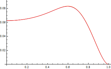
Refer to caption
Figure 1. Function A1​(s)A_{1}(s)
Refer to caption
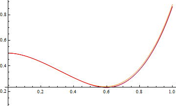
Figure 1. Function B1​(s)B_{1}(s)
Refer to caption
Figure 1. Function A2​(s)A_{2}(s)
Refer to caption
Figure 1. Function B2​(s)B_{2}(s)
Figure 1. The case supp​μ1=[−2,0]\text{\rm{supp}}\,\mu_{1}=[-2,0], supp​μ2=[0,1]\text{\rm{supp}}\,\mu_{2}=[0,1]: Blue plot: computation via the NNRR coefficients; Orange plot: computation via differential equations; Red plot: computation via the algebraically-geometric approach of Section 4.
Refer to caption
Figure 2. Function A1​(s)A_{1}(s)
Refer to caption
Figure 2. Function B1​(s)B_{1}(s)
Refer to caption
Figure 2. Function A2​(s)A_{2}(s)
Refer to caption
Figure 2. Function B2​(s)B_{2}(s)
Figure 2. The case supp​μ1=[−2,0]\text{\rm{supp}}\,\mu_{1}=[-2,0], supp​μ2=[0.25,1]\text{\rm{supp}}\,\mu_{2}=[0.25,1]: Blue plot: computation via recurrence coefficients; Purple plot: computation via differential equations with the boundary conditions at s=0s=0; Green plot: computation via differential equations with the boundary conditions at s=1s=1.

On Fig. 1 we present the numerics in Wolfram Mathematica for the case [α1,β1]=[−2,0][\alpha_{1},\beta_{1}]=[-2,0], [α2,β2]=[0,1][\alpha_{2},\beta_{2}]=[0,1]. In (i) |n→||\vec{n}| was taken 15001500 (blue plot); in (ii) the in-built NDSolve Mathematica function was used (orange plot); notice that the ODE for B1B_{1} in (3.4) has a singular behavior at s=0s=0 and the same is true for B2B_{2} at s=1s=1, so one should use

B1′​(s)=2​C1​(s)+s​C1′​(s)C1​(s)+C2​(s)​(1+C2​(s)C1​(s)),B2′​(s)=2​C2​(s)−(1−s)​C2′​(s)C1​(s)+C2​(s)​(1+C1​(s)C2​(s)),B_{1}^{\prime}(s)=\frac{2C_{1}(s)+sC_{1}^{\prime}(s)}{\sqrt{C_{1}(s)+C_{2}(s)}}\left(1+\frac{C_{2}(s)}{C_{1}(s)}\right),\,B_{2}^{\prime}(s)=\frac{2C_{2}(s)-(1-s)C_{2}^{\prime}(s)}{\sqrt{C_{1}(s)+C_{2}(s)}}\left(1+\frac{C_{1}(s)}{C_{2}(s)}\right),

instead (these follow from  (3.4) and (3.15)); in (iii) the interval s∈[0,1]s\in[0,1] was divided into 30003000 subintervals (red plot). The three plots are effectively indistinguishable.

5.2. Numerics: two non-touching intervals

On Figure 2 we present the limits A1​(s),A2​(s),B1​(s),B2​(s)A_{1}(s),A_{2}(s),B_{1}(s),B_{2}(s) for an Angelesco system with [α1,β1]=[−2,0][\alpha_{1},\beta_{1}]=[-2,0], [α2,β2]=[0.25,1][\alpha_{2},\beta_{2}]=[0.25,1]. The blue plot corresponds to the computation of an→,ja_{\vec{n},j} and bn→,jb_{\vec{n},j} recursively (via  (1.5)–(1.7)) with |n→|=1500|\vec{n}|=1500; the purple plot corresponds to the numerical approximation of the solution to the system of ODE’s (via (3.5)) with the boundary conditions at s=0s=0; the green plot corresponds to the numerical approximation of the solution to the system of ODE’s (via (3.5)) with the boundary conditions at s=1s=1. Equivalently, the purple plot corresponds to the coefficients’ limits for the Angelesco system with supports of μ1\mu_{1} and μ2\mu_{2} being [−2,0.25][-2,0.25] and [0.25,1][0.25,1], while the green plot corresponds to the supports [−2,0][-2,0] and [0,1][0,1]. See Subsection 4.3 for the explanation of this phenomenon. This can also be seen from the fact that (3.6) is independent of β1\beta_{1} and that  (3.7) is independent of α2\alpha_{2}. Again, the plots effectively overlap (away from the plateau regions).

Acknowledgments

The authors are grateful to the anonymous referees for their corrections and careful proof-reading of the paper. The second author thanks W. Van Assche for the excellent mini-course on multiple orthogonal polynomials at the Summer School on OPSF at the University of Kent, which lead to the idea of the current paper. He also thanks the organizers of the Summer School and W. Van Assche and A. Martínez-Finkelshtein for useful discussions.

References

  • [1] A.I. Aptekarev, Spectral Problems of High-Order Recurrences, Amer. Math. Soc. Transl., 233 (2014) 43–61.
  • [2] A. I. Aptekarev, S. A. Denisov, M. L. Yattselev, Self-adjoint Jacobi matrices on trees and multiple orthogonal polynomials, Trans. Amer. Math. Soc., 373 (2) (2020), 875–917.
  • [3] A. I. Aptekarev, M. Derevyagin, W. Van Assche, Discrete integrable systems generated by Hermite–Pade approximants, Nonlinearity, 29 (5) (2016) 1487–1506.
  • [4] A.I. Aptekarev, V. Kalyagin, G. Lopez Lagomasino, I.A. Rocha, On the limit behavior of recurrence coefficients for multiple orthogonal polynomials, J. Approx. Theory 139 (2006) 346–370.
  • [5] A. I. Aptekarev, V. A. Kalyagin, V. G. Lysov, D. N. Toulyakov, Equilibrium of vector potentials and uniformization of the algebraic curves of genus 0, J. Comput. Appl. Math., 233 (3) (2009) 602–616.
  • [6] A. I. Aptekarev, V. A. Kalyagin, E. B. Saff, Higher-order three-term recurrences and asymptotics of multiple orthogonal polynomials, Constr. Approx., 30 (2) (2009) 175–223.
  • [7] A. I. Aptekarev, W. Van Assche, M. L. Yattselev, Hermite-Padé Approximants for a Pair of Cauchy Transforms with Overlapping Symmetric Supports, Communications on Pure and Applied Mathematics, 70 (3) (2017) 444–0510.
  • [8] M. Duits, B. Fahs, R. Kozhan, Global fluctuations for Multiple Orthogonal Polynomial Ensembles, preprint, arXiv:1912.04599.
  • [9] G. Filipuk, M. Haneczok, W. Van Assche, Computing recurrence coefficients of multiple orthogonal polynomials, Numerical Algorithms, 70 (3) (2015) 519–543.
  • [10] A. A. Gonchar and E. A. Rakhmanov, On the convergence of simultaneous Padé approximants for systems of functions of Markov type, Proc. Steklov Inst. Math. 157 (1983) 31–50.
  • [11] V. A. Kaliaguine, On operators associated with Angelesco systems, East J. Approx. 1 (2) (1995) 157–170.
  • [12] V.G. Lysov, D.N. Tulyakov, On a vector potential theory equilibrium problem with the Angelesco matrix of interaction Proc. Steklov Inst. Math., 298 (2017) 170–200.
  • [13] V.G. Lysov, D.N. Tulyakov, On the Supports of Vector Equilibrium Measures in the Angelesco Problem with Nested Intervals Proc. Steklov Inst. Math., 301 (2018) 180–196, https://doi.org/10.1134/S0081543818040144.
  • [14] B. Simon, Szegő’s theorem and its descendants: spectral theory for L2L{{}^{2}} perturbations of orthogonal polynomials, Princeton University Press, 2011.
  • [15] W. Van Assche, Chapter 23, Classical and Quantuum Orthogonal Polynomials in One Variable: in (by M.E.H. Ismail), volume 98 of Encyclopedia of Mathematics and its Applications. Cambridge University Press, 2005.
  • [16] W. Van Assche, Nearest neighbor recurrence relations for multiple orthogonal polynomials, J. Approx. Theory 163 (2011) 1427–1448.
  • [17] W. Van Assche, Ratio asymptotics for multiple orthogonal polynomials, In Modern trends in constructive function theory, Contemp. Math., 661 (2016) 73–85, AMS, Providence, RI.
  • [18] M. Yattselev, Strong asymptotics of Hermite-Pade approximants for Angelesco systems, Canad. J. Math., 68 (5) (2016) 1159–1200, http://dx.doi.org/10.4153/CJM-2015-043-3.