Robustness in power law kinetic systems with reactant-determined interactions
Abstract
Robustness against the presence of environmental disruptions can be observed in many systems of chemical reaction network. However, identifying the underlying components of a system that give rise to robustness is often elusive. The influential work of Shinar and Feinberg established simple yet subtle network-based conditions for absolute concentration robustness (ACR), a phenomenon in which a species in a mass-action system has the same concentration for any positive steady state the network may admit. In this contribution, we extend this result to embrace kinetic systems more general than mass-action systems, namely, power law kinetic systems with reactant-determined interactions (denoted by “PL-RDK”). In PL-RDK, the kinetic order vectors of reactions with the same reactant complex are identical. As illustration, we considered a scenario in the pre-industrial state of global carbon cycle. A power law approximation of the dynamical system of this scenario is found to be dynamically equivalent to an ACR-possessing PL-RDK system.
Keywords. Absolute concentration robustness , Chemical reaction network, Power law kinetics, Reactant-determined interactions, Carbon cycle model
1 Introduction
Robustness may be generally defined [15, 26] as a system-level dynamical property that allows a system to sustain its functions despite changes in internal and external conditions. This feature, in fact, is fundamental and ubiquitous in many biological processes, including cellular networks and entire organisms [2, 15, 26]. One type of robust behavior is “concentration robustness,” wherein some quantity involving the concentrations of the different species in a network is fixed at equilibrium [10]. In a well-cited paper published in Science, Shinar and Feinberg [26] introduced absolute concentration robustness (ACR), a condition in which the concentration of a species in a network attains the same value in every positive steady state set by parameters and does not depend on initial conditions.
Shinar and Feinberg presented sufficient structure-based conditions for a chemical reaction network (CRN) to display ACR on a particular species through a structural index called the deficiency. This non-negative parameter has been the center of many powerful results in Chemical Reaction Network Theory (CRNT), a theoretical body of work that associates the structure of a CRN to the dynamical behaviour of the system [11, 12]. CRNT employs mathematical methods from graph theory, linear algebra, group theory and the theory of ordinary differential equations. In CRNT, chemical reaction networks are viewed as digraphs whose vertices (called complexes) are mapped to non-negative vectors representing compositions of chemical species and whose arcs represent chemical reactions between them. The Shinar-Feinberg Theorem on ACR holds for systems whose evolution are modelled by ordinary differential equations with mass-action kinetics (MAK), and is stated as follows:
Consider a mass-action system that admits a positive steady state and suppose that the deficiency of the underlying reaction network is one. If there are two nonterminal nodes in the network that differ only in species , then the system has absolute concentration robustness in .
Here, we show that this result extends to systems endowed with power law kinetics (PLK), which generalize mass-action kinetics [7, 14]. Several experiments have shown that the kinetic order of a reaction with respect to a given reactant is a function of the geometry within which the reaction occurs [16, 17, 18, 22, 25]. In the case of reactions occurring within a three-dimensional homogenous space (as in mass-action systems), the kinetic order is the same as the number of molecules entering into the reaction. However, for systems characterized by molecular overcrowding (e.g., when other molecules deny the reactants from the supposedly allowable space, and to stickiness, when the reactants are found along the surfaces of the reaction vessel) the kinetic orders for the reactions can exhibit non-integer values [24] found in power law formalism [23, 28, 29]. For instance, in intracellular environments, which are highly structured and characterized by molecular crowding, reactions in vivo are likely to take place on membranes or channels and as such, reactions follow fractal-like kinetics [6, 8, 19, 25]. The presence of power law kinetics in reaction systems thus motivated CRN-based studies on PLK systems ([9, 13, 20, 27] among others), some of which are extensions or modifications of existing results on MAK systems.
This contribution specifically shows that the result of Shinar and Feinberg on ACR applies to a class of PLK system called power law kinetic systems with reactant-determined interactions (denoted by “PL-RDK”). PL-RDK systems are kinetic systems with power law rate functions whose kinetic order vectors are identical for reactions with the same reactant complex. Since the kinetic orders of the mass-action rate functions are precisely the stoichiometric coefficients of the reactant complex, one can see that MAK is a special case of PL-RDK.
As an application, we employ the theorem to a power law approximation of the ODE system corresponding to a specific scenario in the pre-industrial carbon cycle model developed by Anderies et al. [1]. Particulary, for the pre-industrial scenario where there are anthropogenic causes that reduce the capacity of terrestrial carbon pool to store carbon, the power law approximation leads to an ACR-possessing PL-RDK system.
The rest of the paper is organized as follows: Section 2 assembles preliminary concepts in Chemical Reaction Network Theory required in stating and proving the results. Section 3 discusses the extension of the Shinar-Feinberg Theorem on ACR for PL-RDK systems. Section 4 applies the main result obtained from the previous section to a carbon cycle model. In Section 5, we summarize our results and outline some research perspectives.
2 Fundamentals of Chemical Reaction Networks and Kinetic Systems
We recall some fundamental notions about chemical reaction networks (CRNs) and
chemical kinetic systems (CKS) assembled in [5, 27]. Some concepts introduced by Feinberg in [11, 12] are also reviewed.
Notation. We denote the real numbers by , the non-negative real numbers by and the positive real numbers by . Objects in the reaction systems are viewed as members of vector spaces. Suppose is a finite index set. By , we mean the usual vector space of real-valued functions with domain . For , the coordinate of is denoted by , where . The sets and are called the non-negative and positive orthants of , respectively. Addition, subtraction, and scalar multiplication in are defined in the usual way. If and , we define by
The vector ,where , is given by
If , the standard scalar product is defined by
By the support of , denoted by , we mean the subset of assigned with non-zero values by . That is,
Definition 1.
A chemical reaction network (CRN) is a triple of three finite sets:
- 1.
a set of species;
- 2.
a set of complexes;
- 3.
a set of reactions such that for any , and for each , there exists such that either or .
We denote the number of species with , the number of complexes with and the number of reactions with
A CRN can be viewed as a digraph with vertex-labelling. In particular, it is a digraph where each vertex has positive degree and stoichiometry, i.e., there is a finite set of species such that is a subset of . The vertices are the complexes whose coordinates are in , which are the stoichiometric coefficients. The arcs are precisely the reactions.
We use the convention that an element is denoted by . In this reaction, we say that is the reactant complex and is the product complex. Connected components of a CRN are called linkage classes, strongly connected components are called strong linkage classes, and strongly connected components without outgoing arcs are called terminal strong linkage classes. We denote the number of linkage classes with , that of the strong linkage classes with , and that of terminal strong linkage classes with . A complex is called terminal if it belongs to a terminal strong linkage class; otherwise, the complex is called nonterminal.
With each reaction , we associate a reaction vector obtained by subtracting the reactant complex from the product complex . The stoichiometric subspace of a CRN is the linear subspace of defined by
The rank of the CRN, , is defined as .
Many features of CRNs can be examined by working in terms of finite dimensional spaces (species space), (complex space), and (reaction space). Suppose the set forms the standard basis for where or . We recall four maps relevant in the study of CRNs: map of complexes, incidence map, stoichiometric map and Laplacian map.
Definition 2.
Let be a CRN.
- 1.
The map of complexes maps the basis vector to the complex .
- 2.
The incidence map is the linear map defined by mapping for each reaction , the basis vector to the vector .
- 3.
The stoichiometric map is defined as .
- 4.
For each , the linear transformation called Laplacian map is the mapping defined by
where refers to the component of relative to the standard basis.
The following result, named as the Structure Theorem of the Laplacian Kernel (STLK) by Arceo et al. in [5], is crucial in deriving important results in CRNT [11, 12].
Proposition 1 (Structure Theorem of the Laplacian Kernel (STLK), Prop. 4.1 [11]).
Let be a CRN with terminal strong linkage classes . Let and its associated Laplacian. Then has a basis such that for all .
A non-negative integer, called the deficiency, can be associated to each CRN. The deficiency of a CRN, denoted by , is the integer defined by . This index has been the center of many studies in CRNT due to its relevance in the dynamic behaviour of the system. In [11], Feinberg provided a geometric interpretation of deficiency: . From this fact and the STLK, the following result follows.
Corollary 1 (Cor. 4.12 [11]).
Let be a CRN with deficiency and terminal strong linkage classes. Then for each ,
By kinetics of a CRN, we mean the assignment of a rate function to each reaction in the CRN. It is defined formally as follows.
Definition 3.
A kinetics of a CRN is an assignment of a rate function to each reaction , where is a set such that . A kinetics for a network is denoted by
The pair is called the chemical kinetic system (CKS).
The above definition is adopted from [30]. It is expressed in a more general context than what one typically finds in CRNT literature. For power law kinetic systems, one sets . Here, we focus on the kind of kinetics relevant to our context:
Definition 4.
A chemical kinetics is a kinetics satisfying the positivity condition:
Once a kinetics is associated with a CRN, we can determine the rate at which the concentration of each species evolves at composition .
Definition 5.
The species formation rate function of a chemical kinetic system is the vector field
The equation is the ODE or dynamical system of the CKS. A positive equilibrium or steady state is an element of for which . The set of positive equilibria of a chemical kinetic system is denoted by .
Power law kinetics is defined by an matrix , called the kinetic order matrix, and vector , called the rate vector.
Definition 6.
A kinetics is a power law kinetics (PLK) if
with and . A PLK system has reactant-determined kinetics (of type PL-RDK) if for any two reactions , with identical reactant complexes, the corresponding rows of kinetic orders in are identical, i.e., for .
An example of PL-RDK is the well-known mass-action kinetics (MAK), where the kinetic order matrix is the transpose of the matrix representation of the map of complexes [11]. That is, a kinetics is a MAK if
where , called rate constants. Note that pertains to the stoichiometric coefficients of a reactant complex .
Remark 1.
In [5], Arceo et al. discussed several sets of kinetics of a network and drew a “kinetic landscape”. They identified two main sets: the complex factorizable kinetics and its complement, the non-complex factorizable kinetics. Complex factorizable kinetics generalize the key structural property of MAK – that is, the species formation rate function decomposes as
where is the map of complexes, is the Laplacian map, and such that for all . In the set of power law kinetics, PL-RDK is the subset of complex-factorizable kinetics.
We recall the definition of the matrix from the work of Müller and Regensburger [20, 21]: For each reactant complex, the associated column of is the transpose of the kinetic order matrix row of the complex’s reaction, otherwise (i.e., for non-reactant complexes), the column is 0. We form the -matrix of a PL-RDK system by truncating away the columns of the non-reactant complexes in , obtaining an matrix, where denotes the number of reactant complexes [27].
3 Absolute Concentration Robustness in PL-RDK Systems
To illustrate absolute concentration robustness, we consider the following toy model:
| (3.1) |
The map depicts a biochemical system involving transfer of material from two pools: to and to , but with regulating the second process. Suppose the system evolves according to the following set of ODEs:
| (3.2) |
The positive equilibrium of the system is attained when
| (3.3) |
where is the conserved amount of total material. These equations indicate that whenever , a positive steady state exists. Furthermore, since has the same value in any steady state, the system exhibits ACR in .
We define absolute concentration robustness in PL-RDK systems as follows:
Definition 7.
A PL-RDK system has absolute concentration robustness(ACR) in species if there exists and for every other , we have .
The following proposition adapts Theorem S3.15 found in supplementary online material of the paper of Shinar and Feinberg [26] to deal with PL-RDK systems.
Proposition 2.
Let be a deficiency-one CRN. Suppose that is a PL-RDK system which admits a positive equilibrium . If are nonterminal complexes, then each positive equilibrium of the system satisfies the equation
| (3.4) |
We largely reproduce the proof of Shinar and Feinberg in the said supplementary material of their paper. Since in their proof, the sums are often taken over all complexes, we use the notation of Müller and Regensburger in [20, 21]:
adjoining zero columns for the non-reactant complexes, where denotes the number of reactant complexes. Furthermore, we write for .
Proof.
Assume that is a positive steady state of the PL-RDK system . That is,
| (3.5) |
For each , define the positive number by
| (3.6) |
Thus, we obtain
| (3.7) |
Suppose that is also a positive equilibrium of the system. Hence,
| (3.8) |
Define
| (3.9) |
With given by Equation (3.6) and given by Equation (3.9), it follows from Equation (3.8) that
| (3.10) |
Let such that
Observe that Equations (3.7) and (3.10) can be respectively written as
Equivalently,
| (3.11) |
| (3.12) |
Therefore, and are positive equilibria of the PL-RDK system if and only if Equations (3.11) and (3.12) hold. From Corollary 1, we have
| (3.13) |
for the CRN under consideration. Let be a basis for as in Proposition 1 (STLK). Since , this basis of can be extended to form a basis of . Recall from Equation (3.11) that is in . We assert that the set is a basis for (and hence, equality holds in Equation (3.13)). This follows if
| (3.14) |
From Proposition 1, every element of must have its support contained entirely in the set of terminal complexes. However, the support of consists of all complexes. By assumption, there are nonterminal complexes and hence, cannot lie in (i.e., Equation (3.14) holds).
From Equation (3.12), there exist scalars such that
| (3.15) |
The extension of the Shinar-Feinberg Theorem on ACR to PL-RDK systems is stated as follows.
Theorem 1.
Let be a deficiency-one CRN and suppose that is a PL-RDK system which admits a positive equilibrium. If are nonterminal complexes whose kinetic order vectors differ only in species , then the system has ACR in .
Proof.
Suppose and are positive equilibria of the PL-RDK system . Observe that since are nonterminal complexes whose kinetic order vectors differ only in species , we have
for some nonzero . Thus Equation (3.4) reduces to
It follows that
That is, the system has ACR in species . ∎
The ODE system in Equation (3.2) can be translated into a dynamically equivalent CRN with associated kinetic order matrix by employing the notion of total CRN representation of Generalized Mass Action (GMA) systems, proposed by Arceo et al. [5]. GMA system is a canonical framework used in Biochemical Systems Theory (BST) wherein every mass transfer rate is approximated separately with a power law term, and these terms are added together, with a plus sign for incoming fluxes and a minus sign for outgoing fluxes [28, 29]. For BST-related concepts, the reader may refer to the BST tutorial in the Appendix of Arceo et al. [3].
The total CRN representation of a GMA system allows for the CRN-based analysis of the dynamical system. Viewed as a GMA system, the set of ODEs in (3.2) has the following total CRN representation:
| (3.18) |
with associated kinetic order matrix given by
The CRN in (3.18) is a deficiency-one network with nonterminal complexes and whose kinetic order rows differ only in . The previous theorem indicates ACR in , which agrees with the computation in (3.3).
The following simple proposition provides some examples for the ACR theorem for PL-RDK systems. As preparation, we recall some notions from [4, 27] which are used in the result. A PL-RDK is said to be reactant set linear independent (of type PL-RLK) if the columns of are linearly independent. We also recall the reactant matrix , which is obtained from the matrix representation of by removing the columns corresponding to non-reactant complexes. Its image is called the reactant subspace , whose dimension is called the reactant rank of the CRN. The reactant deficiency is the difference between the number of reactant complexes and the reactant rank .
Proposition 3.
Let be a deficiency one reaction network, which with PL-RDK, admits a positive equilibrium. Suppose the network has zero reactant deficiency, two nonterminal complexes differing only in and the map
is given by
Then the system is PL-RLK and has ACR in .
Proof.
Since is an isomorphism, is also an isomorphism. This implies that the system is PL-RLK. The kinetic order vector difference of and is for some nonzero real so that Theorem 1’s condition is fulfilled. ∎
4 Application to a Carbon Cycle Model
The pre-industrial carbon cycle model of Anderies et al. [1] is a simple mass balance which involves three interacting carbon pools: land, atmosphere and ocean. Pictorially, the system can be depicted using a biochemical map comprised of nodes that represent carbon pools, solid arrows that indicate transfer of carbon, and dashed arrows that indicate if a pool affects or modulates a process. Figure 4.1 presents the biochemical map of the model of interest.

In our previous work [13], we reviewed the model’s design and underlying assumptions and described the parameters and ODEs present in the pre-industrial state of the carbon cycle model. We also approximated all rate processes by products of power law functions in order to obtain a GMA system approximation of the original system. The resulting ODEs of the approximation is given in (4.1):
| (4.1) |
We also obtained in [13], using total CRN representation of [5], the following deficiency-one CRN representation for the model:
| (4.2) |
Its associated kinetic order matrix is the transpose of the following -matrix:
| (4.3) |
In the Appendix, it is shown that there is a scenario in the pre-industrial state leading to a GMA system approximation such that the kinetic order vectors of the nonterminal vertices and differ only in ; that is, and . In particular, this occurs when the human terrestrial carbon off-take term (which accounts for human activities that reduce the capacity of terrestrial pool to capture carbon such deforestation and land-use change) vanishes. Assuming the existence of a steady state, Theorem 1 indicates that the system has ACR in . In fact, when , steady state computation of the system in (4.1) yields the following equilibria set for the system:
where total conserved carbon at pre-industrial state.
5 Conclusion and Outlook
In conclusion, we summarize our results and outline some perspectives for further research.
- 1.
We modified the Shinar-Feinberg Theorem on ACR for mass-action systems to include PL-RDK systems, a kinetic system more general than mass-action systems.
- 2.
The theorem is applied to a power law approximation of Anderies et al.’s Earth’s carbon cycle in its pre-industrial state. The analysis reveals that there is a scenario in the pre-industrial state which yields a power law approximation where there is ACR in the atmospheric carbon pool. Specifically, the power law approximation leads to an ACR-possessing PL-RDK system when the human off-take coefficient, which accounts for the which accounts for human activities that reduce the capacity of terrestrial pool to sequester carbon, vanishes.
- 3.
The investigation of other forms of “concentration robustness” identified by Dexter et al. [10] for PL-RDK systems offers a further interesting research perspective.
- 4.
The extension of the stochastic analysis of CRNs with ACR of Anderson et al. [2] for PL-RDK systems is another promising area for further investigation.
Acknowledgements
NTF acknowledges the support of the Department of Science and Technology-Science Education Institute (DOST-SEI), Philippines through the ASTHRDP Scholarship grant and Career Incentive Program (CIP). ARL and LFR held research fellowships from De La Salle University and would like to acknowledge the support of De La Salle University’s Research Coordination Office.
References
- [1] Anderies, J., Carpenter, S., Steffen, W., Rockström, J.: The topology of non-linear global carbon dynamics: from tipping points to planetary boundaries. Environmental Research Letters 8(4), 044–048 (2013)
- [2] Anderson, D.F., Enciso, G.A., Johnston, M.D.: Stochastic analysis of biochemical reaction networks with absolute concentration robustness. J R Soc Interface 11(93) (2014)
- [3] Arceo, C.P.P., Jose, E.C., Lao, A., Mendoza, E.R.: Reaction networks and kinetics of biochemical systems. Mathematical biosciences 283, 13–29 (2017)
- [4] Arceo, C.P.P., Jose, E.C., Lao, A., Mendoza, E.R.: Reactant subspaces and kinetics of chemical reaction networks. Journal of Mathematical Chemistry 56(2), 395–422 (2018)
- [5] Arceo, C.P.P., Jose, E.C., Marín-Sanguino, A., Mendoza, E.R.: Chemical reaction network approaches to biochemical systems theory. Mathematical Biosciences 269, 135–52 (2015)
- [6] Zeljko Bajzer, Huzak, M., Neff, K.L., Prendergast, F.G.: Mathematical analysis of models for reaction kinetics in intracellular environments. Mathematical Biosciences 215(1), 35 – 47 (2008)
- [7] Clarke, B.L.: Stoichiometric network analysis. Cell Biophysics 12, 237–253 (1988)
- [8] Clegg, J.S.: Cellular infrastructure and metabolic organization. In: Stadtman, E.R., Chock, P.B. (eds.) From Metabolite, to Metabolism, to Metabolon. Current Topics in Cellular Regulation, vol. 33, pp. 3–14. Academic Press (1992)
- [9] Cortez, M.J., Nazareno, A., Mendoza, E.: A computational approach to linear conjugacy in a class of power law kinetic systems. Journal of Mathematical Chemistry 56(2), 336–357 (2018)
- [10] Dexter, J.P., Dasgupta, T., Gunawardena, J.: Invariants reveal multiple forms of robustness in bifunctional enzyme systems. Integr. Biol. 7, 883–894 (2015)
- [11] Feinberg, M.: Lectures on chemical reaction networks. Notes of lectures given at the mathematics research center of the University of Wisconsin (1979)
- [12] Feinberg, M.: The existence and uniqueness of steady states for a class of chemical reaction networks. Arch. Ration. Mech. Anal. 132, 311–370 (1995)
- [13] Fortun, N., Lao, A., Razon, L., Mendoza, E.: A deficiency-one algorithm for a power law kinetics with reactant determined interactions. Journal of Mathematical Chemistry 56(10), 2929–2962 (2018)
- [14] Horn, F., Jackson, R.: General mass action kinetics. Arch. Rational Mech. Anal 47, 187–194 (1972)
- [15] Kitano, H.: Biological robustness. Nature Reviews Genetics 5(11), 826–837 (2004)
- [16] Kopelman, R.: Rate processes on fractals: theory, simulations, and experiments. Journal of Statistical Physics 42, 185–200 (1986)
- [17] Kopelman, R.: Fractal reaction kinetics. Science 241 4873, 1620–1626 (1988)
- [18] Kopelman, R., Koo, Y.: Reaction kinetics in restricted spaces. Israel Journal of Chemistry 31(2), 147–157 (1991)
- [19] Kuthan, H.: Self-organisation and orderly processes by individual protein complexes in the bacterial cell. Progress in Biophysics and Molecular Biology 75(1), 1 – 17 (2001)
- [20] Müller, S., Regensburger, G.: Generalized mass action systems: Complex balancing equilibria and sign vectors of the stoichiometric and kinetic-order subspaces. SIAM Journal of Applied Mathematics 72, 1926–1947 (2012)
- [21] Müller, S., Regensburger, G.: Generalized mass-action systems and positive solutions of polynomial equations with real and symbolic exponents (invited talk). In: Proceedings of the International Workshop on Computer Algebra in Scientific Computing(CASC) (2014)
- [22] Newhouse, J.S., Kopelman, R.: Steady-state chemical kinetics on surface clusters and islands: segregation of reactants. The Journal of Physical Chemistry 92(6), 1538–1541 (1988)
- [23] Savageau, M.A.: Biochemical systems analysis: I. some mathematical properties of the rate law for the component enzymatic reactions. American Journal of Science 25(3), 365–369 (1969)
- [24] Savageau, M.A.: Development of fractal kinetic theory for enzyme-catalysed reactions and implications for the design of biochemical pathways. Biosystems 47(1), 9 – 36 (1998)
- [25] Schnell, S., Turner, T.E.: Reaction kinetics in intracellular environments with macromolecular crowding: simulations and rate laws. Progress in biophysics and molecular biology 85 2–3, 235–260 (2004)
- [26] Shinar, G., Feinberg, M.: Structural sources of robustness in biochemical reaction networks. Science 327(5971), 1389–1391 (2010)
- [27] Talabis, D.A.S.J., Arceo, C.P.P., Mendoza, E.R.: Positive equilibria of a class of power law kinetics. Journal of Mathematical Chemistry 56(2), 358–394 (2018)
- [28] Voit, E.: Computational analysis of biochemical systems: a practical guide for biochemists and molecular biologists. Cambridge University Press (2000)
- [29] Voit, E.: Biochemical systems theory: A review. ISRN Biomathematics 2013, 1–53 (2013)
- [30] Wiuf, C., Feliu, E.: Power-law kinetics and determinant criteria for the preclusion of multistationarity in networks of interacting species. SIAM J. Applied Dynamical Systems 12, 1685–1721 (2013)
Appendix A Pre-industrial Carbon Cycle Model of Anderies et al.
The complete set of ODEs for the pre-industrial state is given by
| (A.1) |
where
For the description of the parameters, the reader is referred to [1] and the Appendix of [13]. The parameter values are identical to the values used in [13] but with . This particular parameter is assigned as the human terrestrial carbon off-take rate. It is associated to human activities such as clearing, burning or farming, which reduce the capacity of land to capture carbon.
A power law approximation of the ODE system at an operating point is obtained to generate a Generalized Mass Action (GMA) System [28, 29]. Mathematically, GMA system approximation is equivalent to Taylor approximation up to the linear term in logarithmic space. The function can be approximated by at an operating point where
| (A.2) |
Table presents the four carbon fluxes present in the pre-industrial state of the Anderies et al. model, and their corresponding rate functions. Furthermore, the last column lists their respective target power law approximation. The last two functions, and , are already in the desired format and are thus, kept as is. To compute for the kinetic orders (and rate constants), we apply (A.2). By taking the parameter values used in [13] but with , and assuming the initial values to be , and (as in[1]), the ODE system in (A.1) reaches the following steady state:
| Carbon Flux | Function | Power law approx. |
|---|---|---|
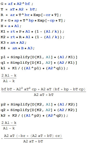
The algebraic calculations are implemented in Mathematica as shown in Figure A.1. When (i.e., the human off-take term vanishes),
For the power law approximation, we choose values close to the equilibrium point as operating point: , and . Consequently, we obtain
| (A.3) |