Dark-State Optical Potential Barriers with Nanoscale Spacing

Optical potentials have been a very useful tool for manipulation of atomic motions, such as simulation of many-body physics Bloch 2005; Bloch et al. 2008. The typical potentials can be generated using a far-detuned light through optical dipole force due to a spatially varying AC-Stark shift Grimm et al. 2000. The potential landscape is determined therefore by the spatial variation of the light intensity. Except operating near the surface Chang et al. 2009; Gullans et al. 2012; Romero-Isart et al. 2013; Thompson et al. 2013; Mitsch et al. 2014; González-Tudela et al. 2015 or using special masks Brezger et al. 1999; Huang and Zheludev 2009, the spatial intensity variation is often limited by the wavelength $\lambda$ of the light. To realize subwavelength resolution in the far field, various approaches have been proposed Gardner et al. 1993; Qi et al. 2012; Yavuz et al. 2009; Liao et al. 2010; Sun et al. 2011; Nascimbene et al. 2015; Yi et al. 2008; Lundblad et al. 2008; Shotter et al. 2008; Berman et al. 1998; Weitz et al. 2004; Salger et al. 2007; Ge et al. 2013; Sahrai et al. 2005; Agarwal and Kapale 2006; Yavuz and Proite 2007; Gorshkov et al. 2008; Kiffner et al. 2008; Li et al. 2008; Mompart et al. 2009; Viscor et al. 2012; Miles et al. 2013, such as multi-tone dressing Yi et al. 2008; Lundblad et al. 2008; Shotter et al. 2008, multi-photon process Berman et al. 1998; Weitz et al. 2004; Salger et al. 2007; Ge et al. 2013, and atomic dark states in $\Lambda$-configurations Sahrai et al. 2005; Agarwal and Kapale 2006; Yavuz and Proite 2007; Gorshkov et al. 2008; Kiffner et al. 2008; Li et al. 2008; Mompart et al. 2009; Viscor et al. 2012; Miles et al. 2013.

Recently, a novel idea of subwavelength optical potentials was proposed by considering the non-adiabatic corrections Dum and Olshanii 1996 to the spatially varying dark states in the $\Lambda$ configurations Lacki et al. 2016; Jendrzejewski et al. 2016. A subwavelength potential barrier arises when the kinetic energy of an atom experiences a rapid change of its internal state in a subwavelength region. This new type of optical potentials is drastically different from the optical dipole potentials as the former is purely quantum mechanical since the potential energy is proportional to $\hbar$. The first experiment of these barriers has been demonstrated Wang et al. 2018. By using standing-waves, the potentials can form lattices with subwavelength barriers spaced by $\lambda/2$. With time-dependent engineering of the lattices, smaller spacings between narrow barriers are possible Subhankar et al. 2019a; Lacki et al. 2019; Tsui et al. 2019. However, heating can arise and the dark-state lifetime can be limited due to lattice modulation Lacki et al. 2019; Tsui et al. 2019.

In this paper, we present a method to create multi-barrier non-adiabatic potentials with subwavelength spacing, realizing a new type of optical potential landscape without time-dependent modulations. Our idea is based on dark-state non-adiabatic potentials of three-level atoms in the $\Lambda$ configurations (Fig. 1 (a)) by controlling the spatial intensity variations on the driving lasers. We employ the Born-Oppenheimer (BO) approximation Dum and Olshanii 1996 to study the internal eigenstates of the atoms and non-adiabatic corrections from the atomic motions. We derive the general formula for the corrections of an arbitrary spatial intensity function. In particular, we show that double barriers and triple barriers with subwavelength spacings can be realized.

Double-barrier potentials have been widely studied in solid-state systems, such as semiconductor heterostructures Goldman et al. 1987; Petukhov et al. 2002; Songmuang et al. 2010. They are important for understanding effects such as resonant tunneling Petukhov et al. 2002 and quasi-bound states Nguyen et al. 2009. Our scheme offers a new platform to study double barriers in cold atoms in the subwavelength regime, where many-body atomic interactions can be strongly enhanced. As an example, we illustrate the formation of bound states of two and three atoms via magnetic dipolar interactions numerically. Our results show that the double-barrier potentials can support bound states of very long lifetime on the order of seconds.

We consider three-level atoms with a $\Lambda$ energy structure shown in Fig. 1 (a). The two ground states $\ket{g_{1}}$ and $\ket{g_{2}}$ are long-lived, which can be hyperfine-split metastable states or Zeeman sublevels Fleischhauer et al. 2005, and an excited state $\ket{e}$ has a spontaneous decay rate $\gamma$. The total Hamiltonian of the system includes the kinetic energy and the internal atomic interaction is given by Lacki et al. 2016 $\mathcal{H}=\frac{p^{2}}{2m}+\mathcal{H}_{\text{in}}$, where

Here $\Omega_{c}(x)$ ($\Omega_{p}(x)$) is the spatial-dependent Rabi frequency of the off-resonant coupling (probe) field for the transition between $\ket{e}$ and $\ket{g_{1}}$ ($\ket{g_{2}}$) with a detuning $\Delta$. These fields form a resonant Raman transition between the ground states Scully and Zubairy 1999. To study the non-adiabatic corrections, we will employ a similar procedure to that in Ref. Jendrzejewski et al. 2016. However, in contrast to the previous works Lacki et al. 2016; Jendrzejewski et al. 2016; Wang et al. 2018; Subhankar et al. 2019a; Lacki et al. 2019, we consider both the coupling and the probe fields to be position dependent, which will lead to general expressions of the non-adiabatic corrections.

We are interested in the limit of slow atomic motions such that the energy of the external motion (the kinetic energy and the potential) is much smaller than the internal energy scale determined by $\mathcal{H}_{\text{in}}$. Within this limit, we can apply the BO approximation Dum and Olshanii 1996 to treat the internal Hamiltonian separately. The validity of this limit will be discussed later. We can diagonalize $\mathcal{H}_{\text{in}}$ and obtain the eigenstates to be

where the corresponding eigenenergies are $0$ and $\hbar\Omega_{\pm}/2$, respectively. Here $\Omega(x)=\sqrt{\Omega^{2}_{c}(x)+\Omega^{2}_{p}(x)}$, $\Omega_{\pm}(x)=-\Delta\pm\sqrt{\Omega^{2}(x)+\Delta^{2}}$. Therefore, the atoms are trapped at the spatially varying dark state $\ket{D(x)}$ and are decoupled from the laser fields Agarwal and Kapale 2006; Yavuz and Proite 2007; Gorshkov et al. 2008; Kiffner et al. 2008.

Since the momentum $p$ and the position $x$ do not commute, additional contributions arise when we diagonalize the kinetic energy using the position-dependent eigenbasis, which are termed as non-adiabatic corrections or geometric potentials Lacki et al. 2016; Jendrzejewski et al. 2016. To see this, we consider the unitary operator Jendrzejewski et al. 2016 $\mathcal{R}=\ket{D(x)}\bra{D_{0}}+\ket{B_{+}(x)}\bra{B_{+0}}+\ket{B_{-}(x)}\bra{B_{-0}},$ where $\ket{D_{0}}$ and $\ket{B_{\pm 0}}$ are the eigenstates located at a fixed position $x_{0}$. By applying the transformation, we obtain

where the effective vector potential $\mathcal{A}\equiv\hbar\mathcal{R}^{\dagger}\partial_{x}\mathcal{R}=i\hbar\alpha^{\prime}(x)\sum_{a=\pm}N_{a}\left(\ket{B_{a0}}\bra{D_{0}}-\ket{D_{0}}\bra{B_{a0}}\right)+i\hbar\frac{\Omega^{\prime}(x)}{\Omega(x)}C\left(\ket{B_{-0}}\bra{B_{+0}}-\ket{B_{+0}}\bra{B_{-0}}\right)$ with $\alpha(x)=\arctan\left[\Omega_{p}(x)/\Omega_{c}(x)\right]$, $N_{\pm}=1/\sqrt{1+\Omega^{2}_{\pm}(x)/\Omega^{2}(x)}$ and $C=(\Delta\Omega/2)/(\Delta^{2}+\Omega^{2})$. Therefore, we arrive at

where the non-adiabatic potential for the dark state is Lacki et al. 2016

It is the nonzero derivative of $\alpha(x)$ that gives rise to potential barriers (positive potential) for the dark state $\ket{D(x)}$. Thus the ratio of the two driving lasers, $f(x)\equiv\Omega_{c}(x)/\Omega_{p}(x)=\tan[\alpha(x)]$, plays an important role in engineering interesting spatial structures of subwavelength barriers. The non-adiabatic potentials for the bright states are $U_{a}=\hbar^{2}/(2m)\left[N_{a}^{2}\alpha^{\prime 2}(x)+C^{2}\Omega^{\prime 2}(x)/\Omega^{2}(x)\right]=N_{a}^{2}U_{0}(x)+4C^{2}U_{1}(x)\leq U_{0}(x)+U_{1}(x)/4,$ where $U_{1}(x)=\hbar^{2}/(8m)\Omega^{\prime 2}(x)/\Omega^{2}(x)$. The off-diagonal contribution that couples between the eigenstates is given by

where $U_{b}(x)=\hbar^{2}/(2m)N_{+}N_{-}\alpha^{\prime 2}(x)$, and $U_{0a}=\pm\hbar^{2}/(2m)N_{\mp}C\alpha^{\prime}(x)\Omega^{\prime}(x)/\Omega(x)$. The coupling rates between the dark state and the bright states are $V_{\pm D}\equiv|\bra{B_{\pm 0}}\mathcal{V}\ket{D_{0}}|/\hbar=|U_{0\pm}(x)|/\hbar$, which determine the loss rate of atoms out of the dark state. We show that $U_{b}(x)\leq U_{0}(x)/2$ and $|U_{0\pm}(x)|\leq\sqrt{U_{0}(x)U_{1}(x)}/2$. To ensure the validity of BO approximation,

In particular, as shown numerically in Fig. 2 (b), $U_{1}(x)\lesssim U_{0}(x)$ around the double barriers. For $|\Delta|\lesssim|\Omega(x)|$, we can reduce Eq. (7) to $U_{0}(x)\ll\hbar|\Omega(x)|$. Under this condition, the off-diagonal coupling $\mathcal{V}$ is far-detuned from the energy spacing between the eigenstates, therefore it can be treated as a perturbation. Then the excitation to the open channels can be estimated Jendrzejewski et al. 2016; Scully and Zubairy 1999 as $P_{B}\sim|\bra{B_{a0}}\mathcal{V}\ket{D_{0}}|^{2}/\Omega^{2}(x)=V^{2}_{\pm D}/\Omega^{2}(x)\ll 1$. The effective loss rate of the dark state atoms is given by $\gamma_{d}\sim\gamma V^{2}_{\pm D}/\Omega^{2}(x)$. A more rigorous result of the dark-state decay rate is calculated from the corrections to the dispersion of atoms in the Bloch bands Lacki et al. 2016, which shows a similar relation to our perturbative result.

The non-adiabatic potential arises due to the rapidly spatial change of the internal dark state. Previous studies Lacki et al. 2016; Jendrzejewski et al. 2016; Wang et al. 2018; Bienias et al. 2018; Subhankar et al. 2019a; Lacki et al. 2019; Tsui et al. 2019 have focused on the situation when the ratio of the coupling laser to the driving laser to be an approximated linear function near certain values, i.e. $f(x)\approx kx/\epsilon$ for $|kx|\lesssim\epsilon$. The non-adiabatic potential for the dark state is given by Jendrzejewski et al. 2016 $U_{0}(x)=\frac{\hbar^{2}k^{2}}{2m\epsilon^{2}}/[1+(kx/\epsilon)^{2}]^{2},$ which shows a single potential barrier located at $x=0$ with $U_{0}(0)=\frac{\hbar^{2}k^{2}}{2m\epsilon^{2}}$ and a width $\Delta x\sim\epsilon/k$. In general, $f(x)$ can be made periodic, e.g. $f(x)=\sin(kx)/\epsilon$ Lacki et al. 2016; Wang et al. 2018, so the separation between two barriers is $\lambda/2$. Recent studies show that the separation can be reduced further via Floquet engineering Subhankar et al. 2019a; Lacki et al. 2019; Tsui et al. 2019.

Here we consider a more general situation of laser intensities as

which can be formed by a combination of standing waves and propagating waves. Here $a,\ b,\ c,\ d,$ are the amplitude coefficients to be determined and $\phi$ is the phase control.

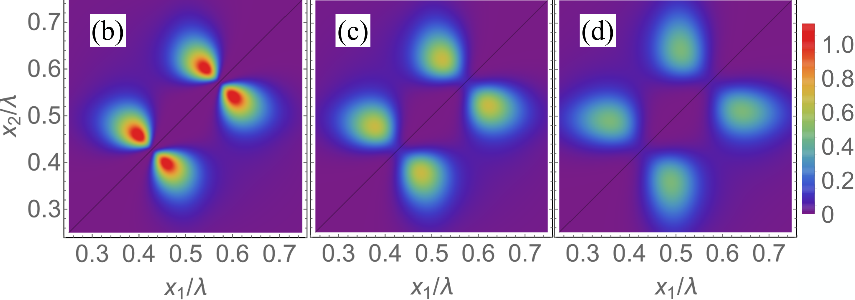
We now discuss a study of many-body physics permitted by the non-adiabatic potential barriers. The spatial-varying dark state may allow the atoms to have spatially dependent magnetic moments Bloch et al. 2008 in the subwavelength regime, leading to strong magnetic dipole-dipole interactions. For concreteness, we assume the magnetic moments are aligned perpendicular to $x-$axis that the atoms are located at. (The situation on transverse position distribution will be discussed later.) The strength of the magnetic moment of an atom is taken to be $\mu(x)=\mu_{m}\left[2P_{g_{1}}(x)-1\right]$, which depends on the state (spin) of the atom, i.e., $P_{g_{1}}(x)$. For the situation of two atoms, the total Hamiltonian is given by Lacki et al. 2016

where $\mu_{0}$ is the vacuum permeability, and $x_{i}$ and $p_{i}$ are the position and the momentum of the $i$th atom.

In the case of the double barriers, the atoms repel each other through the magnetic dipolar interaction if they both stay in the well. Thus a bound state can not be formed. Instead, a bound state can be formed if only one atom sits inside the well. The condition for the bound state is $E_{\min}+\frac{\mu_{0}\mu(x_{1})\mu(x_{2})}{4\pi|x_{1}-x_{2}|^{3}}<0$, where $E_{\min}$ is the minimum energy of the atom inside the potential well and the energy of the other atom outside the well is neglected. By considering the size of the potential well and using the uncertainty principle, we estimate $E_{\min}\approx\hbar^{2}k^{2}/\left[2m\epsilon(1-d)\right]$. Then we estimate the minimum magnetic moment in order to form a bound state, and we find that the required dipolar length $a_{dd}\equiv\mu_{0}\mu^{2}m/\left(12\pi\hbar^{2}\right)$ Lahaye et al. 2009 is on the order of the typical subwavelength spacing, i.e., $a^{\min}_{dd}\sim 0.2\sqrt{\epsilon(1-d)}\lambda\sim\Delta x$.

A more rigorous determination of $a^{\min}_{dd}$ can be obtained by numerically solving the Schördinger equation (12) to have at least one negative eigenvalue. In practice, the dipole-dipole interaction would be modified due to the transverse distribution, and so does $a^{\min}_{dd}$. The dipolar potential in 3D is given by $V_{\text{3D}}=\mu_{0}\mu(x_{1})\mu(x_{2})(r^{2}-3z_{12})/(4\pi r^{5})$ Büchler et al. 2007. Here $r$ is the atomic distance in 3D, and $z_{12}$ is the atomic distance along the $z-$axis, where the dipoles are assumed to be oriented. We assume that each atom is strongly confined in the transverse direction, where its distribution probability for the $j$th atom is given by $P(y_{j},z_{j})=\exp[-(y_{j}^{2}+z_{j}^{2})/l_{T}^{2}]/(4\pi l_{T}^{2})$ with $l_{T}$ the strength of transverse confinement. We first find the effective dipole-dipole interaction by integrating the transverse variables in $V_{\text{3D}}$ using $P(y_{j},z_{j})$, and then solve Eq. (12) using the effective interaction.

We study the dependence of $a^{\min}_{dd}$ shown in Fig. 4 (a). In the ideal case when $l_{T}=0$, we search $a^{\min}_{dd}$ for different values of $\epsilon$ (circular points). Using the critical values of $a_{dd}$, we calculate the average atomic distance along the $x-$axis $\bar{x}_{12}$ from the wave function $\psi(x_{1},x_{2})$. We find that $a^{\min}_{dd}$ increases linearly with $\bar{x}_{12}$ as we change $\epsilon$, i.e., $a^{\min}_{dd}\approx 1.2\bar{x}_{12}\approx 0.55\sqrt{\epsilon}\lambda$, which is close to the value obtained in the analytical method when $d=0$. For $l_{T}=0.10\sqrt{\epsilon}\lambda\ll\bar{x}_{12}$, we find both $\bar{x}_{12}$ and $a_{dd}^{\min}$ increase slightly where $a^{\min}_{dd}\approx 1.5\bar{x}_{12}$ (square points). For $l_{T}=0.20\sqrt{\epsilon}\lambda\approx\bar{x}_{12}/3$, $a^{\min}_{dd}$ is increased to about $3.0\bar{x}_{12}$ (diamond points).

We plot the bound-state probability distributions $|\psi(x_{1},x_{2})|^{2}$ using $a^{\min}_{dd}$ at $\epsilon=1/10$ for $l_{T}=0,\ 0.10\sqrt{\epsilon}\lambda,\ 0.20\sqrt{\epsilon}\lambda$ in Fig. 4 (b)-(d). We observe that there is a high probability to find one atom located inside the potential well while the other outside, so the magnetic moments tend to be close to its maximum magnitude $\mu_{m}$. There is almost zero probability to find atoms sitting close to the domain walls ($x_{j}\approx 4.25$ and $5.75$) where $\mu(x)$ changes signs Lacki et al. 2016, so the contact interaction due to $s$-wave scattering Lahaye et al. 2009 can be neglected.

We also investigate the nonadiabatic potential experienced by the bound-state atoms. Due to the double-barrier potential, the average off-diagonal coupling rate can be very small, which is given by $\int V_{\pm D}(x_{1})|\psi(x_{1},x_{2})|^{2}dx_{1}dx_{2}\leq\int\sqrt{U_{0}(x_{1})U_{1}(x_{2})}/(2\hbar)\psi(x_{1},x_{2})|^{2}dx_{1}dx_{2}\equiv\bar{U}_{\text{off}}/\hbar$. In Fig. 5 (empty squares), we plot this upper-bound of the average off-diagonal coupling potential $\bar{U}_{\text{off}}$ versus the mean atomic distance as $\epsilon$ varies. The results show that $\bar{U}_{\text{off}}\sim E_{R}$, which is two orders of magnitude smaller than the peak nonadiabatic potential $U_{0}(x_{\max})$ in Fig. 5 (circles). The small off-diagonal coupling potential can support very long lifetime of the bound states. We estimate the lifetime of the bound states as $\tau=1/\bar{\gamma}_{d}$, where $\bar{\gamma}_{d}=\gamma\int U_{0}(x_{1})U_{1}(x_{2})/(2\hbar\Omega(x_{1}))^{2}|\psi(x_{1},x_{2})|^{2}dx_{1}dx_{2}$. Using the parameters in Sec. V, we show that lifetime on the order of seconds can be realized at tens of nanometers atomic distance.

Moreover, the double-barrier potential can lead to bound states of three atoms known as trimers. Our trimer has one atom inside the well and two outside on each side of the barrier. Similarly, bound states can be formed in the case of the triple potential barriers. The atoms attract each other if they are separated by the center barrier such that the dipoles are opposite and the magnitude is about $\mu_{m}$ (Fig. 3). With periodic potentials, our multiple barriers can be interesting for the study of many-body physics in band structures, which is out of the scope of this work.

The non-adiabatic potential multiple barriers require the $\Lambda$ atomic configuration and spatial control on the Rabi frequencies. The $\Lambda$ atomic configurations have been frequently used in electromagnetic-induced transparency Fleischhauer et al. 2005 and coherent population transfer Bergmann et al. 1998. The first experiment on non-adiabatic potentials has been performed using an ultracold ¹⁷¹Yb gas Wang et al. 2018 with hyperfine-split ground states.

The spatial dependence on the Rabi frequencies $\Omega_{c}(x)$ and $\Omega_{p}(x)$ is of the form $a+b\cos(kx)$, which can be realized by superposing a standing-wave and a propagating wave derived from the same laser. Thus, the spatial function $f(x)$ is insensitive to the laser intensity fluctuation. As the perfect spatial function may be challenge in experiment, a double barrier can be more easily demonstrated with an approximated function $f(x)=(x-x_{\min})^{2}/\epsilon$ by shaping the coupling and the probe lasers.

We can determine the minimum barrier spacing from $U_{0}(x)\ll\hbar|\Omega(x)|$. The minimum value of the Rabi frequency is $\Omega(x)=\sqrt{\Omega_{c}^{2}(x)+\Omega_{p}^{2}(x)}\approx\Omega_{0}\epsilon(1-d)$ for the double-barrier potentials, and $\Omega(x)\approx\Omega_{0}\left[1-\cos^{2}(\phi)\right]\approx\Omega_{0}\phi^{2}/2$ for the triple-barrier potentials. Considering $\Omega_{0}=2\pi\times 100$ MHz, $\lambda=532$ nm, and $U_{0}(x)\leq\hbar|\Omega(x)|/5$ for ¹⁷¹Yb atoms, we obtain the minimum barrier spacing to be $13$ nm and $24$ nm for the double-barrier potentials and the triple-barrier potentials, respectively. The corresponding minimum energy inside the double barriers is $E_{\min}/\hbar\approx 2\pi\times 280$ kHz. We estimate the maximum excitation probability is $P_{B}\approx 4\%$. Taking $\gamma=2\pi\times 182$ kHz Wang et al. 2018, we find the scattering rate on the dark states through the open channel is about $2\pi\times 7$ kHz. In the above analysis, we assumed $|\Delta|\lesssim|\Omega(x)|$, however, for larger single-photon detunings, the laser intensities need to be stronger in order to get the same subwavelength feature without breaking the BO approximations.

In this work, we presented a method of creating non-adiabatic potentials of multiple barriers separated at tens of nanometers via spatial engineering of the laser intensities. The ability of spatial control could potentially open a new direction to engineer interesting subwavelength potential landscapes. We studied several concrete examples on realizing subwavelength multiple barriers and their application for bound states. Interestingly, we show that double-barrier potentials can support bound states of very long lifetimes.

The multiple barriers can be a new platform for the study of many-body interactions in cold atoms enhanced by the subwavelength features. This scheme may also allow further studies on trapping atoms without the conventional optical dipole potentials and super-resolution quantum microscopy McDonald et al. 2019; Subhankar et al. 2019b.