The First Maps of – the Dust Mass Absorption Coefficient – in Nearby Galaxies, with DustPedia2019The First Maps of – the Dust Mass Absorption Coefficient – in Nearby Galaxies, with DustPedia–
Abstract
The dust mass absorption coefficient, is the conversion function used to infer physical dust masses from observations of dust emission. However, it is notoriously poorly constrained, and it is highly uncertain how it varies, either between or within galaxies. Here we present the results of a proof-of concept study, using the DustPedia data for two nearby face-on spiral galaxies M 74 (NGC 628) and M 83 (NGC 5236), to create the first ever maps of in galaxies. We determine using an empirical method that exploits the fact that the dust-to-metals ratio of the interstellar medium is constrained by direct measurements of the depletion of gas-phase metals. We apply this method pixel-by-pixel within M 74 and M 83, to create maps of . We also demonstrate a novel method of producing metallicity maps for galaxies with irregularly-sampled measurements, using the machine learning technique of Gaussian process regression. We find strong evidence for significant variation in . We find values of at 500 µm spanning the range 0.11–0.25 in M 74, and 0.15–0.80 in M 83. Surprisingly, we find that shows a distinct inverse correlation with the local density of the interstellar medium. This inverse correlation is the opposite of what is predicted by standard dust models. However, we find this relationship to be robust against a large range of changes to our method – only the adoption of unphysical or highly unusual assumptions would be able to suppress it.
Keywords:
galaxies: ISM – galaxies: general – ISM: dust – ISM: abundances – submillimetre: ISM – methods: observational1 Introduction
Interstellar dust provides an indispensable window for studying galaxies and their evolution. Dust, which primarily emits in the Mid-InfraRed (MIR) to Far-InfraRed (FIR) to submillimetre (submm) wavelength regime, can be observed in very large numbers of galaxies very rapidly, with the beneficial effects of negative -correction enhancing our ability to detect dusty galaxies out to high redshift (Eales et al. 2010a; Oliver et al. 2012). This has made dust a standard proxy for studying galaxies’ star-formation (Kennicutt 1998; Buat et al. 2005; Kennicutt et al. 2009), gas mass (Eales et al. 2012; Scoville et al. 2014; Lianou et al. 2016), and chemical evolution (Rowlands et al. 2014; Zhukovska 2014; De Vis et al. 2017a; De Vis et al. 2017b; De Vis et al. 2019) – which are otherwise difficult and time-consuming to observe directly.
However, many of the valuable insights that dust can provide rest upon one simple expectation – that we are able to use observations of dust emission to actually infer physical dust masses. Unfortunately, astronomers remain terrible at this. This is due to the fact that (variously called the dust mass absorption coefficient, or the dust mass opacity coefficient), the wavelength-dependent conversion factor used to calculate dust masses from FIR–submm dust Spectral Energy Distributions (SEDs), is extremely poorly constrained.
a The plotted values of include the values given in the compilation tables of Alton et al. 2004 and Demyk
et al. 2013, along with the values reported by: Ossenkopf &
Henning 1994; Agladze et al. 1996; Weingartner &
Draine 2001; James et al. 2002; Draine 2003; Dasyra et al. 2005; Draine &
Li 2007; Eales
et al. 2010b; Ormel et al. 2011; Compiègne
et al. 2011; Draine
et al. 2014; Gordon
et al. 2014; Planck
Collaboration et al. 2014; Köhler et al. 2015; Jones et al. 2016; Roman-Duval et al. 2017; Bianchi
et al. 2017; Demyk
et al. 2017a; Demyk
et al. 2017b; Chiang et al. 2018.
b The choice of reference wavelength has negligible (< 0.1 dex) effect on the standard deviation of the literature values in the plot, as long as µm.
c Changing to any value in the standard range of 1–2.5 has negligible (< 0.05 dex) effect on the standard deviation of the literature values in the plot.
is essentially a convenience factor, amalgamating the various properties of dust grains that dictate their emissivity – such as the distributions of size, morphology, density, and chemical composition. These individual properties are extremely hard to constrain observationally, and highly degenerate with each other in their effect upon dust emission (Whittet 1992); combining them in allows them to be considered in terms of their net effect. Dust emission in the FIR–submm regime is traditionally modelled as a Modified BlackBody (MBB; or, ‘greybody’), where the observed flux density at wavelength is described by:
| (1) |
where is the distance to the source of the dust emission, is the number of dust components being modelled, is the mass of dust component , is the value of at wavelength for dust component , and is the Planck function evaluated at wavelength for temperature of dust component . While the dust population of a source will in reality span a continuum of temperatures, availability of FIR–submm data typically forces observers to fit their data with only 1 or 2 components (although point-process methods are starting to provide a way to model dust in a more continuous manner; see Marsh et al. 2015; Marsh et al. 2017).
The value of can be estimated in various ways, usually by some combination of: consideration of the elemental constituents of dust (derived from depletions); physical modelling of possible grain structures; chemical modelling of likely dust compositions; radiative transfer modelling; analysis of Ultraviolet (UV) to Near-Infra-Red (NIR) extinction and scattering; laboratory analysis of artificial dust grain analogues; and examination of retrieved grains of interplanetary and interstellar dust. For a fuller summary, and compilation of references, see Section 1 of Clark et al. 2016. Troublingly, the various methods that have been employed for estimating yield a very wide range of possible values. In order to directly compare different values of , they need to be converted to the same reference wavelength. This can be done using the formula:
| (2) |
where is the value of at a particular wavelength , is the value of at a reference wavelength , and is the dust emissivity spectral index. Laboratory analysis of dust analogues and chemical modelling suggest that this relation is reliable in the wavelength range µm; at wavelengths shorter than this the variation of with wavelength becomes much more complex, whilst at longer wavelengths the behaviour of is less clear, with some evidence of an upturn (Demyk et al. 2017a; Demyk et al. 2017b; Ysard et al. 2018).
Figure 1 compiles a wide range of values that have been reported in the literature (all have been converted to a reference wavelength of 500 µm as per Equation 2; we only plot values for which the original quoted reference wavelength was in the reliable 150–1000 µm range). Over 100 values are plotted, with a standard deviation of 0.8 dex, and spanning a total range of over 3.6 orders of magnitude. Worse still, there is no sign that values of reported in the literature are converging over time.
So, despite the excellent sensitivity and wavelength coverage provided by modern FIR–mm observatories, any dust masses inferred from observed dust emission remain enormously uncertain, stymieing our understanding of the InterStellar Medium (ISM) in galaxies. Moreover, this high degree of uncertainty means that, out of necessity, is often treated as being constant – even though it is well understood that this can’t be true in reality. Even the more complex, multi-phase dust model frameworks, such as those of Jones et al. 2013; Jones et al. 2017, usually only incorporate 2 or 3 types of dust, each with a corresponding .
As such, understanding how kappa varies – both between different galaxies, and within individual galaxies – is clearly vital for the field.
In this paper, we use an empirical method for determining the value of – which we employ on a resolved, pixel-by-pixel basis in two nearby galaxies – to produce the first maps of how varies within galaxies, as a proof-of-concept study. The theory behind the dust-to-metals method we employ to find is described in Section 2. The galaxies and data we use in this work are described in Section 3. The application of the technique to produce maps of is Section 4. Our results are presented in Section 5, and are discussed in Section 6. For brevity and readability, ‘flux density’ will be termed ‘flux’ throughout the rest of the paper.
2 Theory
Of the many methods proposed for estimating the value of , one of the most simple is that first proposed by James et al. 2002. The James et al. 2002 method is entirely empirical, and relies upon just one central assumption – that the dust-to-metals ratio in the ISM, , has a known value. If the ISM mass of a galaxy is known, along with the metallicity of that ISM, it is straightforward to calculate the total mass of interstellar metals in that galaxy; then, by assuming a fixed dust-to-metals ratio, it is possible to infer a galaxy’s dust mass a priori, without any reference to the dust emission. This a priori dust mass can then be compared to that galaxy’s observed dust emission, and hence can be calibrated. Here we use the notation for the dust-to-metals ratio, instead of . This maintains consistency with James et al. 2002 and Clark et al. 2016, and avoids any ambiguity arising from the fact that is often used to denote a dust-to-metals ratio normalised by the Milky Way value, whereas our quoted dust-to-metals ratios are always absolute values.
The vast majority of all reported values of lie in the range 0.2–0.6 (considering only values of that are not based upon some assumed value of : Issa et al. 1990; Luck & Lambert 1992; Whittet 1992; Pei 1992; Meyer et al. 1998; Dwek 1998; Pei et al. 1999; Weingartner & Draine 2001; James et al. 2002; Kimura et al. 2003; Draine et al. 2007; Jenkins 2009; Peeples et al. 2014; McKinnon et al. 2016; Wiseman et al. 2017; Telford et al. 2019). As such, it seems fair to conclude that is significantly better constrained than – making the former a useful tool for pinning down the value of the latter. And whilst some authors suggest larger values of (for instance De Cia et al. 2013, who find values in the region of 0.8), we can at least be confident that, by definition, no galaxy has a dust-to-metals ratio greater than 1 – no such helpful constraint exists for . Furthermore, thanks to observations of elemental depletions in the neutral ISM, can be determined far more directly than .
Clark et al. 2016 built upon the James et al. 2002 method, to correct for a number of systematics that affected that original implementation, and to enable it to take advantage of higher-quality modern FIR–submm data. In this work, we apply the Clark et al. 2016 iteration of the dust-to-metals method on a resolved basis, in nearby galaxies. Therefore, for completeness, we here provide a cursory description of the technique as implemented in this work; for a full derivation and description, refer to Section 2 of Clark et al. 2016. The final form of the method can be rendered as the following formula for computing for the ISM of a source:
| (3) |
where is a correction factor to account for the fraction of ISM mass due to elements other than hydrogen, is the atomic hydrogen mass, is the molecular hydrogen mass, is the dust-to-metals ratio, and is the ISM metal mass fraction. The term corresponds to the model used to fit the observed dust emission of the target source – in this instance, MBBs, as per Equation 1; is the number of dust components being modelled, is the flux emitted at wavelength by dust component , and is the Planck function evaluated at wavelength for temperature of dust component ; our SED-fitting procedure is described in Section 4.2.
The formulation in Equation 3 gives a combined value, that incorporates the contribution from all dust species present, for each temperature component (for ). The problem becomes unconstrained if each dust component is treated as having a different . The potential impact of line-of-sight mixing of dust components at different temperatures is discussed in Section 4.2.
The correction factor is required in Equation 3, as the dust-to-metals method is concerned with the total mass of the ISM, not just the mass of hydrogen. It is standard in the literature to account for mass other than hydrogen by applying a fixed factor of 1.36 – corresponding to the Milky Way helium abundance. However this fails to consider how helium abundance varies with galaxy evolution, or the contribution of metals to the mass of the ISM. Thus is defined as:
| (4) |
where is the primordial helium mass fraction, and describes the evolution of the helium mass fraction with metallicity. We use from Aver et al. 2013, and from Balser 2006. Given Equation 4, can therefore vary from 1.33 (for low-metallicity galaxies where 0) to 1.45 (for high-metallicity giant ellipticals where ).
It is important to note that measurements trace gas-phase metallicity in the ionised phase (predominantly Hii regions), whereas we are concerned with the metallicity of the ISM at large. This means that we must account for the fraction of interstellar oxygen mass in Hii regions depleted onto dust grains, , and hence missed by gas-phase metallicity estimators. We use a value of from Mesa-Delgado et al. 2009, which is in good agreement with numerous other reported values (Peimbert & Peimbert 2010; Kudritzki et al. 2012; Bresolin et al. 2016). Whilst the oxygen depletion factor in the ISM at large is known to vary by at least 0.3 dex (Jenkins 2009), oxygen depletion in Hii regions is found to be remarkably constant, at 1.3 (ie, 0.1 dex) across nearby galaxies (evaluated by comparing abundances in Hii regions to abundances in the atmospheres of nearby B stars; Bresolin et al. 2016 and references therein). Additionally, given that the elemental composition of oxygen-rich dust is found to exhibit minimal variation at intermediate-to-high metallicities (Mattsson et al. 2019), the assumption of a constant is valid modulo a constant – which is the central premise of our method.
Atomic hydrogen mass, (in ), is determined using observations of the 21 cm hyperfine structure line, according to the standard prescription:
| (5) |
where is the velocity-integrated flux density of the 21 cm line (in ), and the source distance is here in units of pc.
The mass of molecular hydrogen associated with a source cannot be determined directly from emission; because the molecule is non-polar, it does not radiate when in the ground state (which is the case for the bulk of molecular hydrogen in galaxies). Instead, molecular hydrogen masses are typically inferred by treating CO as a tracer molecule, via observations of the (1-0) rotational line (referred to as CO(1-0) hereafter). The mass of molecular hydrogen, (in ), can thus be calculated using the relation:
| (6) |
where is the velocity-integrated main-beam brightness temperature of the CO(1-0) line (in ), is the CO-to- conversion factor (in ), is the angular diameter of the target source, and the source distance is here in units of pc. The value of is a matter of much debate, but the standard Milky Way value is , which is treated as uncertain by a factor of 2 (see Obreschkow & Rawlings 2009, Saintonge et al. 2011, Bolatto et al. 2013, and references therein). Note that Equation 6 is simply the standard mass surface-density prescription, (where is in units of ), rendered in terms of for consistency with Equations 3 and 5. The CO-to- conversion factor can alternatively be expressed as , which is in terms of column number density density of molecules, being related to according to .
The galaxies considered in this work contain environments with metallicities that vary by a factor of 2.5, spanning 0.4–1 (see Section 4). When considering locales with significantly-varying metallicities, it is important to account for the corresponding variation of with metallicity (Bolatto et al. 2013). In lower-metallicity environments, there will be reduced abundances of C and O, relative to H. Additionally, there is less dust available in low-metallicity environments to shield the CO – which is less able to self-shield than – from photodisassociation (see Wolfire et al. 2010, Clark & Glover 2015, and references therein). Here we opt to use the metallicity-dependent prescription of Amorín et al. 2016, described by:
| (7) |
where is the ISM metallicity in terms of the Solar value, and is an empirical power-law index with a value of .
The Amorín et al. 2016 rule is calibrated on a sample of galaxies spanning over an order of magnitude in metallicity (), by using the Star Formation Efficiency (SFE) and Star Formation Rate (SFR) to infer the molecular gas supply present. They do this by employing the relation ; effectively inverting the Kennicutt-Schmidt law (Kennicutt 1998) to infer the molecular gas mass present, anchored by the known star formation efficiency of the Milky Way. Resolved studies such as Bigiel et al. 2011 and Utomo et al. 2019 find remarkably little variation in SFE within face-on local normal spirals like those studied in this work; this supports the reliability of using a SFE-calibrated method for estimating in a resolved study such as ours. Additionally, the Amorín et al. 2016 prescription effectively traces the median of the commonly-cited metallicity-dependent literature prescriptions (see Figure 11 of Amorín et al. 2016 and Figure 6 of Accurso et al. 2017 for comparisons of prescriptions), making it the choice most likely to not conflcit with other works.
Regarding the Solar metallicity, we use the canonical value for the Solar oxygen abundance of (Asplund et al. 2009), corresponding to a Solar metal mass fraction of (Asplund et al. 2009, uncertainty deemed to be negligible). In common with the literature at large, we assume that oxygen abundance traces total metallicity. Whilst this assumption has its limits, oxygen is the most abundant metal in the Universe, and a dominant constituent of dust (Savage & Sembach 1996; Jenkins 2009), making it a useful metallicity tracer for our purposes. Although the ratio of oxygen to carbon (the other main constituent of dust by mass) is known to vary with metallicity (Garnett et al. 1995), this systematic trend is no more prominent than the intrinsic scatter over the 0.4–1.0 metallicity range relevant to this work (Pettini et al. 2008; Berg et al. 2016).
Although a term appears in Equation 3, the and terms are also both proportional to , which therefore ultimately cancels out. This renders the resulting values of independent of distance, removing a potentially large source of uncertainty.
Throughout this work, when employing values from the literature, we take care to only use values that do not themselves rely upon any assumed value of .
For the value of the dust-to-metals ratio, , in Equation 3, we take two approaches. For our fiducial analysis, presented in Section 5, we assume a constant value of . This is smaller than the value of 0.5 assumed in Clark et al. 2016, as more recent works (McKinnon et al. 2016; De Cia et al. 2016; Wiseman et al. 2017) suggest that for most galaxies with metallicities > 0.1 , the dust-to-metals ratio is slightly below the Milky Way’s average value of 0.5 (James et al. 2002; Jenkins 2009).
The assumption of a constant dust-to-metals ratio is an approximation that will break down at some point. Therefore, in Section 6.2.1, we construct an alternate analysis where increases as a function of ISM surface density. This is a more physical treatment, as depletion of ISM metals onto dust grains is found to increase in regions of greater ISM column density (Jenkins 2009; Roman-Duval et al. 2019). This is in agreement with the fact that grain growth in the ISM is required to explain the dust budgets in many galaxies (Galliano et al. 2008; Rowlands et al. 2014; Zhukovska 2014). As a result, dust grain growth in denser ISM (with the corresponding increase in ) is a feature of dust evolution models such as The Heterogeneous dust Evolution Model for Interstellar Solids (THEMIS; Jones et al. 2013; Jones et al. 2017; Jones 2018). Unfortunately, the exact form of the relationship between and ISM (surface) density is very poorly constrained (the relationship we assume for our analysis is described in detail in Section 6). As such, the variable- model represents a more-physical, but worse-constrained approach; whilst the fixed- model represents a less-physical, but better-constrained approach. For this reason, whilst the fixed- approach is our fiducial model, we nonetheless consider both scenarios.
3 Data


| M 74 | M 83 | |
| NGC No | NGC 628 | NGC 5236 |
| RA (J2000) | 24.174° | 204.254° |
| (01h 36m 41 8) | (13h 37m 01 0) | |
| Dec (J2000) | +15.783° | -29.866° |
| (+15°46′ 58 8) | (-29° 51′ 57 6) | |
| Distance (Mpc) a | 10.1 | 4.9 |
| Hubble Type | SAc | SBc |
| (5.2) | (5.0) | |
| (arcmin) | 10.0 | 13.5 |
| (kpc) | 29.4 | 19.2 |
| () | 683 | 290 |
| () b | 10.1 | 10.5 |
| () c | 9.9 | 10.0 |
| () d | 9.4 | 9.5 |
| () e | 7.5 | 7.4 |
| SFR () b | 2.4 | 6.7 |
| FUV (mag) | 2.9 | 3.4 |
| NUV (mag) | 2.5 | 2.8 |
a As a first-order estimate of the uncertainty on the distance, we use the standard deviation of the redshift-independent distances listed in the Nasa/ipac Extragalactic Database (NED; https://ned.ipac.caltech.edu/ui/) for each galaxy. This gives uncertainties of 3.2 and 3.4 Mpc for M 74 and M 83 respectively.
b Nersesian
et al. 2019.
c Hi mass from total single-dish flux in the HI Parkes All Sky Survey (HIPASS; Meyer
et al. 2004; Wong
et al. 2006).
d This work (see Section 3.4).
e This work (using the pixel-by-pixel values calculated in produced 5).
An initial attempt by Clark et al. 2016 to detect variation in using the dust-to-metals method was unsuccessful; however, that study only considered the global dust properties of galaxies, and considered a sample of 22 objects, all of which were of similar masses, metallicities, and environments. A promising avenue for finding variation in is to look within well-resolved nearby galaxies. Many studies have found that dust properties can vary significantly – and sometimes dramatically – within galaxies (Smith et al. 2012; Roman-Duval et al. 2017; Relaño et al. 2018). It would be surprising if this variation did not extend to .
Creating a map of a galaxy using the dust-to-metals method requires resolved data for its dust emission, atomic gas, molecular gas, and metallicity; with the resolution provided by modern observations, it is possible to make many hundreds, or even thousands, of independent determinations within a galaxy. For this proof-of-concept demonstration we map within two nearby face-on spiral galaxies – M 74 (NGC 628) and M 83 (NGC 5236). We select these galaxies on account of their particularly extensive metallicity data (see Section 3.3), coupled with their resolution-matched multi-phase ISM observations (see Section 3.4).
We obtained the bulk of the necessary data from the DustPedia archive11 1 https://dustpedia.astro.noa.gr/. DustPedia (Davies et al. 2017) is a European Union project working towards a comprehensive understanding of dust in the local Universe, capitalising on the legacy of the Herschel Space Observatory (Pilbratt et al. 2010). A centrepiece of the project is the DustPedia database, which includes every galaxy observed by Herschel that has recessional velocity within ( 40 Mpc), has optical angular size in the range 1′ < < 1°, and has a detected stellar component22 2 As defined according to detection by the Wide-Field Infrared Survey Explorer (WISE; Wright et al. 2010), at its all-sky sensitivity, in 3.4 µm (its most sensitive band)..
The continuum data we employ is described in Section 3.2, the metallicity data (and the process by which we use it to create metallicity maps) is described in Section 3.3, and the atomic & molecular gas data in Section 3.4.
3.1 Target Galaxies
We selected M 74 and M 83 as the subject galaxies for this work; a summary of their basic characteristics is provided in Table 1. Both are very nearby, highly extended, and almost perfectly face-on, making them two of the most heavily-studied galaxies in the sky, and ideally suited to serving as our proof-of-concept targets for mapping .
Both galaxies are classified as ‘grand design’ (Elmegreen & Elmegreen 1987) type Sc spirals, with M 83 also displaying a prominent bar (de Vaucouleurs et al. 1991). M 74 has a physical diameter of 29 kpc – similar to that of the Milky Way (Goodwin et al. 1998; Rix & Bovy 2013) – and about 50% greater than that of M 83 (diameter defined according to the optical , being the isophotal major axis at which the optical surface brightness falls beneath 25 ).
Despite being the physically smaller of the two, M 83 has a stellar mass 2.2 times greater, and a Star Formation Rate (SFR) 2.7 times greater (Nersesian et al. 2019). M 83 has a correspondingly higher surface brightness in dust emission, averaging 4.2 at 500 µm within its , compared to 1.6 for M 74. The nuclear region of M 83 is currently undergoing a bar-driven starburst, concentrated in the central 250 pc, accounting for 10% of the galaxy’s total ongoing star-formation (Sérsic & Pastoriza 1965; Harris et al. 2001; Fathi et al. 2008). The optical disc of M 83 has a minimal systematic metallicity gradient, with oxygen abundances varying by only about 0.1 dex from place to place; in contrast, M 74 has a pronounced metallicity gradient, with oxygen abundances in its centre about 0.3 dex greater than at its (De Vis et al. 2019).
Many of the differences between M 74 and M 83 – such as in their stellar surface densities (and therefore interstellar radiation fields), star formation characteristics, metallicity profiles, ISM distributions, etc – have the potential to affect dust properties, and thereby provide useful scope for us to contrast how can vary due to a range of factors.
The appearances of both galaxies, in various parts of the spectrum, are illustrated in Figures 2 and 3. The stellar masses and SFRs for the DustPedia galaxies, as presented in Nersesian et al. 2019, were estimated using the Code Investigating GALaxy Emission (CIGALE; Burgarella et al. 2005; Noll et al. 2009) software, incorporating the THEMIS dust model.
3.2 Continuum Data
Multiwavelength imagery and photometry for the DustPedia galaxies (spanning 42 ultraviolet–millimetre bands), along with distances, morphologies, etc, are presented in Clark et al. 2018. Our analysis makes use of observations from several of the facilities included in the DustPedia archive.
In the submm, we use observations at 250, 350, and 500 µm from the Spectral and Photometric Imaging REceiver (SPIRE; Griffin et al. 2010) instrument onboard Herschel. In the FIR, we use observations at 160, and 70 µm from the Photodetector Array Camera and Spectrometer (PACS; Poglitsch et al. 2010) instrument, also onboard Herschel (PACS did not perform 100 µm observations for M 83, so for consistency we make no use of the the PACS 100 µm data for M 74). In the MIR, we use observations at 22 µm from the WISE33 3 Whilst 24 µm Spitzer data does exist for these galaxies, the background is better-behaved in the WISE data, thanks to the superior mosaicing permitted by the larger field of view.. A compilation of the MIR–FIR–submm data for each galaxy is shown in the centre-left panels of Figures 2 and 3.
Although not required for the creation of the maps, we use various additional data for reference and comparison, also drawn from the DustPedia archive. This includes UltraViolet (UV) observations from GALaxy Evolution eXplorer (GALEX; Morrissey et al. 2007); UV, optical, and NIR observations from the Sloan Digital Sky Survey (SDSS; York et al. 2000; Eisenstein et al. 2011); optical observations from the Digitized Sky Survey (DSS); plus NIR observations from the InfraRed Array Camera (IRAC; Fazio et al. 2004) and Multiband Imager for Spitzer (MIPS; Rieke et al. 2004) instruments onboard the Spitzer Space Telescope (Werner et al. 2004). A compilation of the UV–optical–NIR data for each galaxy is shown in the far-left panels of Figures 2 and 3.
3.3 Metallicity Data
Galaxies sufficiently extended to have well-resolved global FIR–submm observations, atomic gas observations, and molecular gas observations, are generally too extended to have their UV–NIR nebular spectral emission – and hence metallicities – fully mapped by Integral Field Unit (IFU) spectrometry. Whilst some large-area IFU surveys of nearby galaxies have now been undertaken, these are still very much the exception rather than the rule, and even the very largest can currently only cover 50% of the area of galaxies as extended as M 74 and M 83. (Rosales-Ortega et al. 2010; Sánchez et al. 2011; Blanc et al. 2013). As such, the few DustPedia galaxies with mostly complete IFU coverage do not have the well-resolved gas and dust data needed for this analysis.
However, extended nearby galaxies are popular targets for spectroscopic observation; most have had large numbers of individual slit and fibre spectra taken, supplementing partial IFU coverage like that described above. For DustPedia, De Vis et al. 2019 have compiled a sizeable database of emission line fluxes, collated from 42 literature studies plus all available archival Multi Unit Spectroscopic Explorer (MUSE; Bacon et al. 2010) data that covers the DustPedia galaxies. The De Vis et al. 2019 spectroscopic database contains emission line fluxes from 10,000 spectra, with data for 492 (56%) of the DustPedia galaxies. De Vis et al. 2019 also present consistent gas-phase metallicity measurements for all of these spectra, for 5 different strong-line relation prescriptions (all of which yield standard metallicities). Following their tests of the internal consistency of the prescriptions considered, De Vis et al. 2019 find the Pilyugin & Grebel 2016 ‘S’ prescription most reliable; we therefore use these metallicities throughout the rest of this work. A recent study by Ho 2019 also supports the validity of the Pilyugin & Grebel 2016 prescriptions at the metallicities of our target galaxies. As an additional test, we also repeat the entire -mapping process using metallicity data produced using 4 other strong-line relations; this is presented in Appendix F.
M 74 and M 83 both have large numbers of metallicities in the De Vis et al. 2019 database – 510 and 793 measurements respectively, more than any other DustPedia galaxy (except UGC 09299, which lacks the resolved gas data we require). These metallicity points sample the entirety of both galaxies’ optical discs. The positions of these spectra, and the metallicities derived from them, are plotted in the upper-left panels of Figures 5 and 6. Our region of interest for each galaxy44 4 The region of interest being the area where we map ; illustrated in Figures 2 and Figure 3, and defined in Section 4.1. extends approximately out to 0.55 for M 74, and to 0.7 for M 83. So whilst the bulk of the metallicity points lie within the region of interest of each galaxy, providing dense sampling, there are also sufficient points outside it to constrain the metallicity variations over larger scales.
In order to produce maps of , it was necessary to first have maps of the metallicity distributions of our target galaxies. The first step towards achieving this was modelling their radial metallicity profiles. The spectra metallicity points for M 74 and M 83, plotted as a function of their deprojected galactocentric radius, , are shown in Figure 4. As can be seen, there is significant scatter around the radial trends of both galaxies, far in excess of what would be expected if it were driven solely by the uncertainties on the individual metallicity points. Indeed, if one fits a naïve metallictiy profile where the only variables are the gradient and the central metallicity, then the majority of datapoints would count as > ‘outliers’ in M 83 (and most would count as > outliers for M 74). This scatter represents localised variations in metallicity, which are not azimuthally-symmetric – and which therefore cannot be captured by a 1-dimensional model. Such variation becomes apparent when sampling the metallicity within galaxies at such high spatial resolution (Rosales-Ortega et al. 2010; Moustakas et al. 2010). For example, note the localised region of significantly depressed metallicity in the western part55 5 Centred at approximately: , . of the disc of M 83, visible in the upper-left panel of Figure 6.
| M 74 | M 83 | |
|---|---|---|
| () | ||
| () | ||
| (dex) |
We had to take this intrinsic scatter into account when modelling the radial metallicity profiles of our target galaxies; we therefore used a model with 3 parameters: the metallicity gradient (in ), the central metallicity (in ), and the intrinsic scatter (in dex). We employed a Bayesian Monte Carlo Markov Chain (MCMC) approach to fit this model, the full details of which are given in Appendix A; the resulting parameter estimates, with uncertainties, are listed in Table 2.
It would technically be possible to create metallicity maps of our target galaxies using only these fitted radial metallicity profiles. However, using this simple 1-dimensional approach (ie, where metallicity varies only as a function of ) leads to very large uncertainties on the metallicity value of each pixel in the resulting maps, thanks to the considerable intrinsic scatter values ( for M 74, and for M 83). In contrast, most of the individual spectra metallicity datapoints have uncertainties much smaller than this, with median uncertainties of 0.010 and 0.025 dex for M 74 and M 83 respectively (NB, spectra located in close proximity tend to have metallicities that are in good agreement – see the densely-sampled area in Figures 5 and 6). In other words, there are many areas of these galaxies where the metallicity is known to much greater confidence than is reflected by the global radial metallicity gradient – therefore, relying upon the global 1-dimensional model alone would mean ‘throwing away’ that information. As such, we opted to model the metallicity distributions of our target galaxies in 2 dimensions. To achieve this, we employed Gaussian process regression.
3.3.1 Gaussian Process Regression


Gaussian Process Regression (GPR) is a form of probabilistic interpolation, that makes it possible to model a dataset without having to assume any sort of underlying functional form for the model. GPR (and Gaussian process methodology in general) is a commonly-applied tool in the field of machine learning – and in recent years GPR has seen increasing use in astronomy, to tackle problems where stochastic (and therefore impractical to model directly) processes give rise to complex features in data (for instance, capturing the effect of varying detector noise levels in time-domain data). For a full introduction to Gaussian process methodology, including GPR, see Rasmussen & Williams 2006; for an extensive list of works where Gaussian processes have been successfully applied to problems in astronomy, see Section 1 of Angus et al. 2018.
Instead of trying to model the underlying function that gave rise to the observed data, GPR models the covariance between the datapoints. The covariance is modelled using a kernel, which describes how the values of datapoints are correlated with one another, as a function of their separation in the parameter space.
This covariance-modelling approach is well-suited to the problem we face with mapping metallicity within our target galaxies. Spectra located very close together (eg, within a few arcseconds) will tend to have very similar metallicities, whilst spectra with greater separations (eg, arcminutes apart) will only be weakly correlated with one another (this is readily apparent from visual inspection of Figures 5 and 6).
For the covariance function, we used a Mátern kernel (Stein 1999). The Mátern function is a standard choice for modelling the spatial correlation of 2-dimensional data (Minasny & McBratney 2005;Rasmussen & Williams 2006; Cressie & Wikle 2011) – especially physical data (Schön et al. 2018). In practice, a Mátern kernel is similar to a Gaussian kernel, but has a narrower peak (allowing it to be sensitive to variations over short distances) whilst also having thicker tails (letting it maintain sensitivity to the covariance over large distances). Like a Gaussian, the tails extend to infinity. The Mátern kernel has two hyperparameters: kernel scale, and kernel smoothness (essentially how ‘sharp’ the peak of the kernel is).
Once the covariance has been modelled, it is used in combination with the observed data to trace the underlying distribution. The result is a full posterior Probability Distribution Function (PDF) for the likely value of the underlying function at that location. The uncertainties in each input datapoint are fully considered by GPR. In regions where the input datapoints have large uncertainties, or where datapoints in close proximity disagree with one another, the output PDF will be less well constrained, reflecting the greater uncertainty on the underlying value at that location.
3.3.2 Metallicity Maps Via Gaussian Process Regression
We opted to apply the GPR to the residuals between the individual spectra metallicity points and the global radial metallicity profile (ie, Figure 4). By fitting to the residuals, the global radial metallicity profile effectively serves as the prior for the regression. The regression then traces the structure of the local deviations from the global radial metallicity profile. In regions where there are no data points, the GPR therefore tends to revert to the metallicity implied by the global radial profile.
This process is illustrated in the upper-right panels of Figures 5 and 6 for M 74 and M 83 respectively. The circular points mark the positions of the individual spectra metallicities, colour-coded to show the residual of each (the median absolute residual is 0.026 dex for both galaxies). The coloured background shows the Gaussian process regression to these residuals, similarly colour-coded. We used GaussianProcessRegressor, the GPR implementation of the Scikit-Learn machine learning package for python (Pedregosa et al. 2011). The hyperprior for the kernel scale was flat, but limited to a range of 0.05–0.5 , to prevent the modelled regression being either featurelessly smooth, or unrealistically granular. The kernel smoothness hyperprior was set to 1.5, which is a standard choice due to being computationally efficient, differentiable, and often found to be effective in practice (Rasmussen & Williams 2006; Gatti 2015).
The final metallicity map for each galaxy was produced by adding the residual distribution traced by the GPR to the global radial metallicity profile, for each pixel. The resulting metallicity maps are plotted as contours in the lower-right panels of Figures 5 and 6, for M 74 and M 83 respectively. Visual inspection indicates that the GPR does a good job of tracing the metallicity distribution as sampled by the spectra metallicity points (ie, the contours consistently have the same levels as the points they pass through).
Our full procedure for calculating the uncertainty on the GPR metallicity in each pixel is presented in Appendix B. The resulting metallicity uncertainty maps are shown in the lower-left panels of Figures 5 and 6.
We validated the reliability of the metallicities predicted by GPR by performing a jackknife cross-validation analysis, which is described in detail in Appendix C. This analysis found that the predicted values exhibit no significant bias, and the associated uncertainties are reliable.
There are areas in both galaxies where the datapoints suggest a steadily-increasing residual in a certain direction; the GPR then extrapolates that this increase continues for some distance (defined by the modelled kernel scale) into regions where there are no datapoints. For instance, in the south-western part of M 74, the datapoints suggest that the metallicity gradient is steeper than for the rest of the galaxy (ie, a trend of increasingly negative residuals) – the GPR extrapolates that this increased steepness will continue for a certain distance into an area where there are no metallicity points. A similar situation occurs in the north-west portion of M 83 (but instead with a positive residual). Naturally, extrapolations such as these are highly uncertain; but this is quantified by the uncertainty on the regression at these locations. This is illustrated in the lower-left panels of Figures 5 and 6, which show the uncertainty for each pixel’s predicted metallicity.
Utilising GPR provides a marked reduction in the uncertainty of our metallicity maps, relative to using the global radial metallicity profiles alone. If we were to use that simple global approach, every pixel in our metallicity map for M 74 would have an uncertainty at least as large as the intrinsic scatter of 0.044 dex (Table 2). In contrast, with our GPR metallicity map of M 74, 91% of the pixels within the region of interest4 have uncertainties < 0.044 dex; the median GPR uncertainty within this region is only 0.016 dex. Similarly, whereas the intrinsic scatter on the global radial profile of M 83 is 0.048 dex, the median error on the GPR metallicity map is only 0.037 dex within the region of interest; the GPR uncertainty is less than the global intrinsic scatter for 66% of the pixels within this region.
There exist ‘direct’ electron temperature metallicity measurements for M 74, produced by the CHemical Abundances Of Spirals (CHAOS; Berg et al. 2015). Electron temperature metallicities are at reduced risk of systematic errors, compared to strong-line values like those provided by De Vis et al. 2019. However, the CHAOS data for M 74 only consists of 45 measurements. Whilst we trialled producing metallicity maps with this data, the sparse sampling meant that the uncertainty on the metallicity at any given point was extremely large. Maps of produced with these metallicity maps (as per the procedure described in Section 4) were so dominated by the resulting noise that they were not informative.
3.4 Atomic & Molecular Gas Data
Atomic and molecular gas data for a sample of extended, face-on spiral galaxies in DustPedia – including those studied in this work – is presented in Casasola et al. 2017. For both of our target galaxies, we followed Casasola et al. 2017 and use Hi data from The HI Nearby Galaxy Survey (THINGS, Walter et al. 2008), which conducted 21 cm observations of 34 nearby galaxies with the Very Large Array, at 6--16″ resolution. We retrieved the naturally-weighted moment 0 maps for M 74 and M 83 from the THINGS website66 6 https://www.mpia.de/THINGS/Overview.html. The Hi maps for both galaxies are shown in the 3rd panels of Figures 2 and 3.
To obtain CO observations for M 74 we again followed Casasola et al. 2017, and used data from the HERA Co Line Extragalactic Survey (HERACLES; Leroy et al. 2009), which performed CO(2-1) observations of 18 nearby galaxies using the IRAM 30 m telescope, at 13″ resolution. We retrieved the moment 0 maps, as associated uncertainty maps, from IRAM’s official HERACLES data repository77 7 https://www.iram-institute.org/EN/content-page-242-7-158-240-242-0.html. The CO(2-1) map for M 74 is shown in the 4th panel of Figure 2.
Although M 74 has been observed in CO(1-0) by various authors (Young et al. 1995; Regan et al. 2001), these observations are all lacking in either resolution, sensitivity, and/or coverage, in comparison to the HERACLES data. We therefore found it preferable to use the CO(2-1) data of HERACLES, despite the fact this requires applying a line ratio, , in order to find , and hence calculate mass as per Equation 6.
In nearby late-type galaxies, has an average value of 0.7 (Leroy et al. 2013; Casasola et al. 2015; Saintonge et al. 2017). However, it is also known that varies significantly with galactocentric radius (Casoli et al. 1991; Sawada et al. 2001; Leroy et al. 2009). As such, accurately inferring the CO(1-0) distribution in M 74 using the HERACLES CO(2-1) map required a radially-dependent . To produce this, we used the data presented in Figure 34 (lower-right panel) of Leroy et al. 2009, where they compare the HERACLES maps to literature maps of the same galaxies produced by several other telescopes (with appropriate corrections applied to account for differences in spatial and velocity resolution). This yielded 450 directly-measured values, spanning radii from 0–0.55 , for 9 of the HERACLES galaxies. Leroy et al. 2009 simply binned these points to trace the radial variation in ; however, we chose to take a fully probabilistic approach, and use GPR to infer the underlying radial trend in . In Figure 7, we plot all of the points from Figure 34 (lower-right panel) of Leroy et al. 2009. We applied a GPR to this data, using a Mátern covariance kernel. Because is a ratio, we constructed the regression so that the output uncertainties are symmetric in logarithmic space; otherwise, output uncertainties symmetric in linear space would extend to unphysical values of at larger radii. The resulting regression is shown in black in Figure 7. It is in excellent agreement with the radial trend that Leroy et al. 2009 traced by binning the data, with elevated to 1 in the galaxies’ centres, falling to 0.7–0.8 over the rest of the sampled region – but our approach has the added benefit over binning of providing well-constrained uncertainties on values produced using the regression. The uncertainty associated with the regression is a factor of 1.3 over the range in radius sampled by the HERACLES measurements, reflecting the intrinsic scatter present in the datapoints; beyond this, the uncertainty steadily increases, reaching a factor of 2 at . Given the uncertainty on , this does not represent a large addition to the total uncertainty on the molecular gas masses we calculated.
M 83 was not observed by HERACLES. So we instead used the CO(1-0) observations presented in Lundgren et al. 2004, which were made using the Swedish–Eso Submillimetre Telescope (SEST) at a resolution of 42″, to a uniform depth of 74 mK (). The CO(1-0) map for M 83 is shown in the far-right panel of Figure 3.
4 Application
4.1 Data Preparation
We background-subtracted all continuum maps following the procedure described in Clark et al. 2018, using the background annuli they specify for our target galaxies.
All data (continuum observations, gas observations, and metallicity maps) were smoothed to the resolution of the most poorly-resolved observations for each galaxy. This was done by convolving each image with an Airy disc kernel of Full-Width Half-Maximum (FWHM) given by . We therefore convolve all of our M 74 data to the 36″ resolution of the Herschel-SPIRE 500 µm observations. Likewise, we convolved all of our M 83 data to the 42″ resolution of the SEST Hi observations.
We reprojected all of our data to a common pixel grid for each galaxy, on an east–north gnomic tan projection. We wished to preserve angular resolution, ensuring that our data remain Nyquist sampled, to maximise our ability to identify any spatial features or trends in our final maps. We therefore used projections with 3 pixels per convolved FWHM. This corresponds to 12″ pixels for M 74, and 14″ pixels for M 83.
For each galaxy, we defined a region of interest, within which all required data is of sufficient quality to effectively map . We defined this as being the region within which all pixels in the smoothed & reprojected versions of the Hi map, CO map, and 22–500 µm continuum maps, have SNR > 2 (as defined by comparison to their respective uncertainty maps). For both M 74 and M 83, the data with the limiting sensitivity are the CO observations. The borders of our regions of interest for both galaxies are shown in the far-right panels of Figures 2 and 3.
4.2 SED Fitting
As described in Section 2, the dust-to-metals method lets us establish dust masses a priori; then, by comparing this a priori dust mass to observed FIR–submm dust emission, we can calibrate the value of . This necessitates having a model that describes that FIR–submm dust emission. We wished to minimise the scope for potentially-incorrect model assumptions to corrupt our resulting values. We therefore modelled the dust emission with the simplest model that is able to fit FIR–submm fluxes – a one-component MBB (ie, Equation 1, with ). A one-component MBB model has been shown by many authors to break down in various circumstances (eg: Jones 2013; Clark et al. 2015; Chastenet et al. 2017; Lamperti et al. accepted). However, these primarily concern either submillimetre excess in low-metallicity and/or low-density environments (which are not present in the regions of interest within our target galaxies), the emission from hotter dust components at short wavelengths (which we do not attempt to model; see below), or features only discernable in spectroscopy (which we are not employing). In ‘normal’ galaxies, a one-component MBB can be expected to fit FIR–submm fluxes successfully (Nersesian et al. 2019).
Note that, as a test, we also repeated the entire SED fitting process described in this section with a two-component MBB model (ie, Equation 1, with , giving dust components at two temperatures). However, when comparing the values of both sets of fits, we found that adopting the two-component MBB approach adds little benefit to the quality of the fits. The median reduced values (of all posterior samples, from all pixels) for the one-component MBB fits were 0.61 for M 74 and 0.94 for M 83 – compared to 0.59 and 0.65 respectively for the two-component fits. This indicates that the two-component MBB fits offer minimal improvement over the one-component fits (and, indeed, may be straying into the realm of over-fitting). Given our desire to employ the simplest applicable model, we therefore opt to proceed with the one-component MBB approach for this work. Nonetheless, in Appendix G, we verify that the choice of one- or two-component SED fitting does not result in considerable changes to our overall results.
By performing our SED fitting pixel-by-pixel, we are reducing the degree to which there will be contributions from multiple dust components at different temperatures. Nonetheless, there will inevitably be some degree of line-of-sight mixing of dust populations. This risk will be greatest in the densest regions, where fainter emission from colder, but potentially more massive, dust components can be dominated by brighter emission from warmer, but less massive, components heated by star-formation (Malinen et al. 2011; Juvela & Ysard 2012). If this does occur, then the resulting values will, in effect, factor in the mass of any cold dust component too faint to affect the SED (assuming the a priori dust masses calculated by the dust-to-metals method are accurate). In this scenario, the values we calculate may not be valid if applied to observations with good enough spatial resolution that line-of-sight mixing becomes negligible.
Although we use Equation 1 to model SEDs, we assign an arbitrary value of during the fitting process (as, of course, the SED fitting is being performed in order to allow us to find a value of using the results). This means that the ‘mass’ parameter yielded by our SED fitting merely serves as a normalisation term for the SED amplitude. This is not a problem, as the only output values actually required is the temperature of the dust, and its flux at the reference wavelength; these are needed in Equation 3 to calculate values of .


We also incorporate a correlated photometric error parameter, , into our SED-fitting. The photometric calibration uncertainty of the Herschel-SPIRE instrument contains a systematic error component that is correlated between bands (Griffin et al. 2010; Bendo et al. 2013; Griffin et al. 2013). This arises from the fact that Herschel-SPIRE was calibrated using observations of Neptune; however, the reference model of Neptune’s emission has a uncertainty. We account for this by parameterising the correlated Herschel-SPIRE error as . The scale of accounts for the majority of the combined 5.5% calibration uncertainty of Herschel-SPIRE88 8 SPIRE Instrument & Calibration Wiki: https://herschel.esac.esa.int/twiki/bin/view/Public/SpireCalibrationWeb. As such, for high-SNR sources (such as bright pixels within our target galaxies), where the photometric noise is minimal, the correlated calibration error can actually dominate the entire uncertainty budget. Moreover, the error on does not follow the Gaussian or Student’s distribution typically assumed for photometric uncertainties – rather, it is essentially flat, with the true value of the correlated systematic error almost certainly lying somewhere within the range (Bendo et al. 2013; A. Papageorgiou, priv. comm.; C. North, priv. comm.). Explicitly handling as a nuisance parameter allows us to properly account for this with a matching prior. Gordon et al. 2014 highlight the significant differences that can be found in dust SED fitting when the correlated photometric uncertainties are considered, compared to when they are not.
The Herschel-PACS instrument also has a systematic calibration error, of , arising from uncertainty on the emission models of its calibrator sources, a set of 5 late type giant stars (Balog et al. 2014). However, the error budget on the emission models is dominated by the uncertainty on the line features in the atmospheres of the calibrator stars (see Table 2 of Decin & Eriksson 2007), which are different in each band, and hence not correlated. Only the uncertainty on the continuum component of the emission model, of –, will be correlated between bands. Given the small scale of this correlated error component, and given that systematic error makes up a smaller fraction of the total Herschel-PACS calibration uncertainty than it does for Herschel-SPIRE, and given that the greater instrumental noise for Herschel-PACS means that calibration uncertainty makes up a small fraction of the total photometric uncertainty budget than it does for Herschel-SPIRE, we opt to not model the correlated uncertainty for Herschel-PACS as we do with .
Our one-component MBB SED model therefore has 4 variables: the dust temperature, ; the dust ‘mass’ normalisation, ; the emissivity slope, ; and the correlated photometric error in the Herschel-SPIRE bands, .
The resulting likelihood function, for a set of fluxes (in Jy), observed at a set of wavelengths (in m), with a corresponding set of uncertainties (in Jy), for a set of size , takes the form:
| (8) |
where, for the th wavelength in the set, is the flux arising from dust emission given the SED model parameters, and is the corresponding uncertainty; is a th-order Student distribution99 9 Standardised to allow modes and widths other than zero, as per the SciPy (Jones et al. 2001) implementation: https://docs.scipy.org/doc/scipy/reference/generated/scipy.stats.t.html, centred at a mode of , with a width of . The expected dust emission is given by:
| (9) |
We treat photometric uncertainties as being described by a 1st-order (ie, one degree of freedom) Student distribution. The Student distribution has more weight in the tails than a Gaussian distribution, allowing it to better account for outliers. This makes the Student distribution a standard choice for Bayesian SED fitting (da Cunha et al. 2008; Kelly et al. 2012; Galliano 2018).
For the photometric uncertainty in each pixel, we used the values provided by the uncertainty maps, added in quadrature to the calibration uncertainty of each band: 5.6% for WISE 22 µm1010 10 WISE All-Sky Release Explanatory Supplement (Cutri et al. 2012): https://wise2.ipac.caltech.edu/docs/release/allsky/expsup/sec4_4h.html, 7% for Herschel-PACS 70--160 µm1111 11 PACS Instrument & Calibration Wiki: https://herschel.esac.esa.int/twiki/bin/view/Public/PacsCalibrationWeb, and 2.3%1212 12 2.3% being the non-correlated component of the Herschel-SPIRE calibration uncertainty, separate from . for Herschel-SPIRE 250–500 µm8. Both of our target galaxies lie in regions with negligible contamination from Galactic cirrus. The WISE and Herschel-PACS backgrounds are dominated by instrumental noise, whilst the Herschel-SPIRE background has a significant contribution from the confused extragalactic background. Therefore, for the Herschel-SPIRE data, we also add in quadrature the contribution of confusion noise; for this we use the values given in Smith et al. 2017, of 0.282, 0.211, 0.105 at 250, 350, and 500 µm respectively, derived from the Herschel-ATLAS fields (although the instrumental noise level still dominates over this in all of our Herschel-SPIRE data).
We treat fluxes at wavelengths < 100 µm as upper limits, as emission in this regime will include contributions from hot dust and stochastically heated small grains (Boulanger & Perault 1988; Desert et al. 1990; Jones et al. 2013) that will not be accounted for by our MBB model. Therefore at these wavelengths, any proposed model flux that falls below the observed flux will be deemed as likely as the observed flux itself (ie, no proposed model will be penalised for under-predicting the flux in these bands). Only for proposed model fluxes greater than the observed flux will the likelihood decrease according to the Student distribution, as per usual.
We sample the posterior probability distribution of the SED model parameters in each pixel using the emcee (Foreman-Mackey et al. 2013) MCMC package for python. We perform 750 steps with 500 chains (‘walkers’); the first 500 steps from each chain were discarded as burn-in, and non-convergence was checked for using the Geweke diagnostic1313 13 Comparing the means of the last 90–100% quantile of the combined chains to the 50–60% quantile. (Geweke 1992). Our priors are detailed in Appendix D.
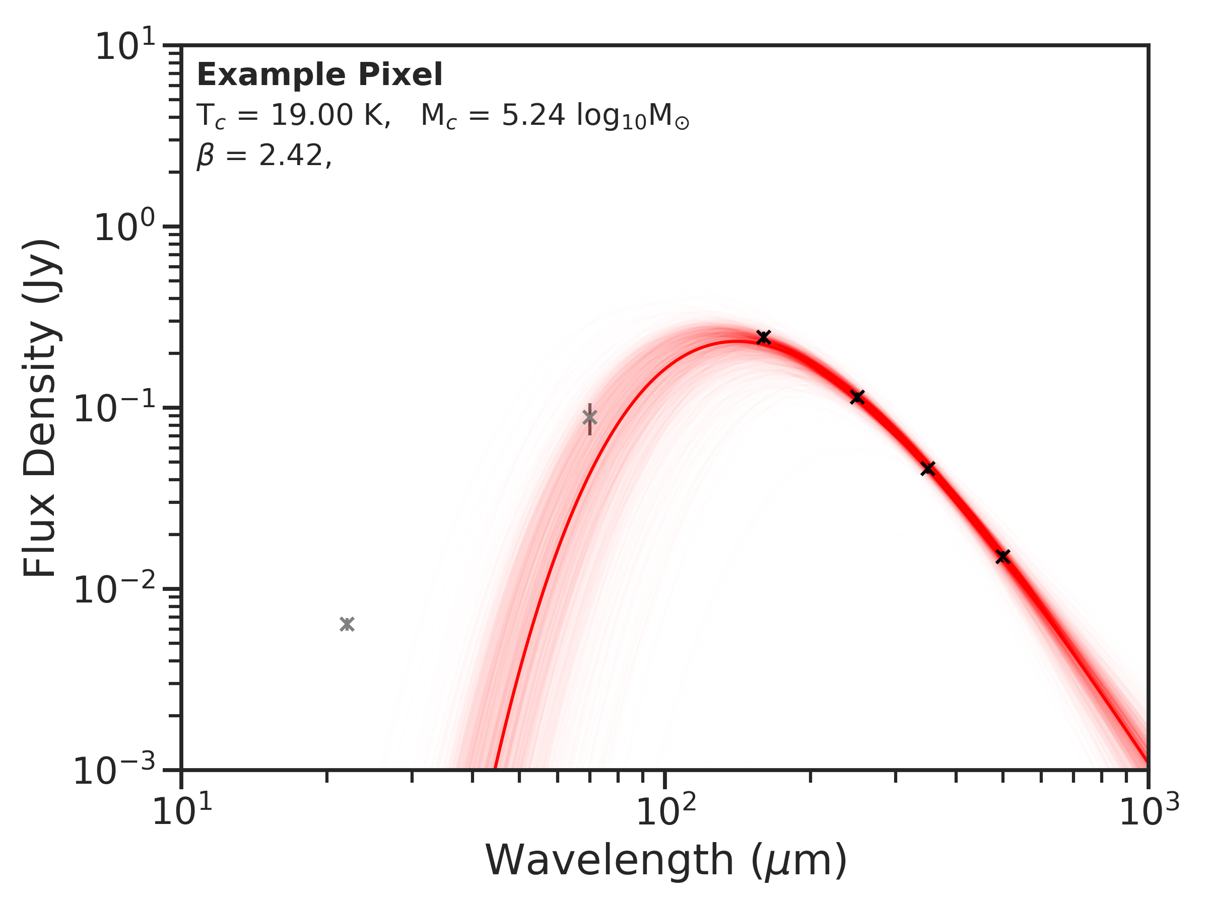
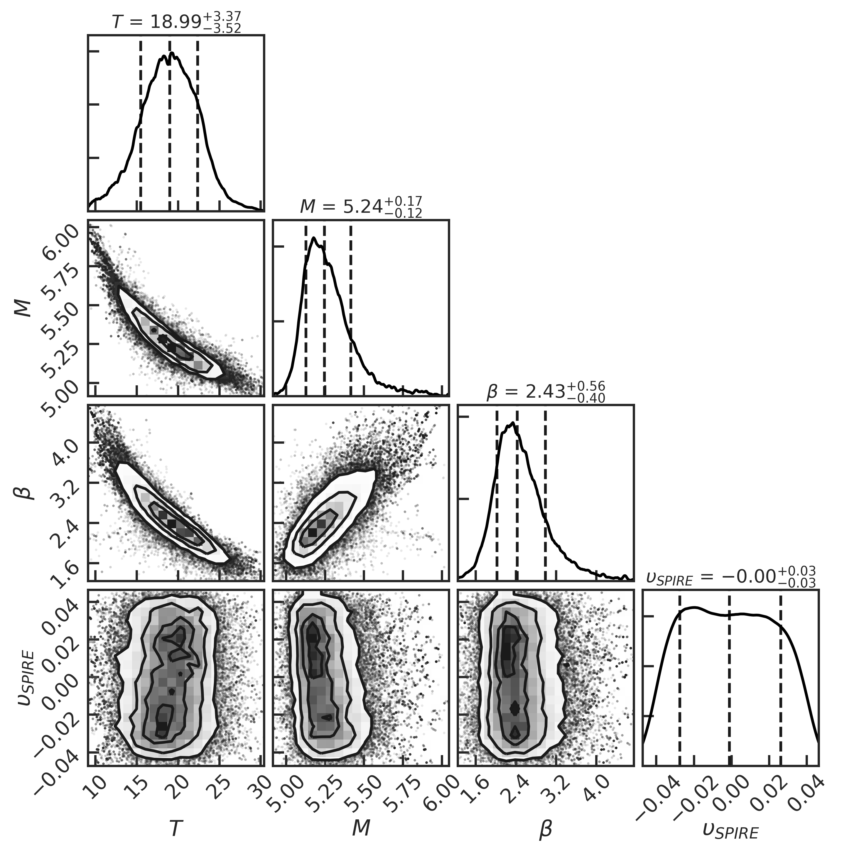
Our SED fitting routine incorporates colour-corrections to account for the effects of the instrumental filter response functions and beam areas1414 14 WISE colour corrections from Wright et al. 2010.,1515 15 Spitzer-MIPS colour corrections from the MIPS Instrument Handbook, version 3 (Colbert 2011): https://irsa.ipac.caltech.edu/data/SPITZER/docs/mips/mipsinstrumenthandbook/51/#_Toc288032329,1616 16 Herschel-PACS colour corrections from the PACS Handbook, version 4.0.1 (Exter et al. 2019): https://www.cosmos.esa.int/documents/12133/996891/PACS+Explanatory+Supplement,1717 17 Herschel-SPIRE colour corrections from the SPIRE Handbook, version 3.1 (Valtchanov et al. 2017): https://herschel.esac.esa.int/Docs/SPIRE/spire_handbook.pdf. An example posterior SED, along with the corresponding parameter distributions, are shown in Figures 8 and 9.
Figures 10 and 11 show maps of the median values of dust mass surface density, temperature, and values for each pixel. We assume that the low temperatures and large values found in the centre of M 83 are non-physical, and instead are due to non-thermal emission from the nuclear starburst affecting the SED-fitting. This is limited to a beam-sized area, consisting of 9 pixels - we therefore exclude these pixels from analysis in later sections, where noted.
Unsurprisingly, the maps of dust mass surface density closely match the morphology of the dust emission (see Figures 2 and 3). The temperature map for M 74 is ‘blotchy’, with warmer dust being located around areas of particularly active star formation (compare to the regions of bright MIR emission in Figure 2 in the northern and southern parts of the disc). The temperature map for M 83 more visibly traces the overall spiral structure; in particular, elevated temperatures are found on the exterior edges of the spiral arms. The maps for both galaxies show correlations with the dust mass surface density; in M 74 this manifests as a broad global trend of beta decreasing with radius, whilst in M 83 beta again more obviously traces the spiral structure.
There is a well-known anticorrelation between temperature and when performing MBB SED fits (Shetty et al. 2009; Kelly et al. 2012; Galliano et al. 2018). This is clearly in evidence in Figure 9. However, as demonstrated by Smith et al. 2012, this does not introduce systematic errors into the results of such fits. And given this lack of systematic bias, the anticorrelation will not introduce spurious trends into resolved SED fits – because fits separated by more than one beam-width will be independent, and will be no more likely to be biased one way than the other. Combined with the fact that we sample the full posterior in our SED fits, and propagate this into the final calculation of our maps (see Section 5), we do not believe that the temperature- anticorrelation will compromise the validity of our final results.
Our SED fitting code has been made freely available online as a python 3 package1818 18 https://github.com/Stargrazer82301/ChrisFit.
5 Results


We now have the atomic gas, molecular gas, metallicity, and dust emission data necessary for every pixel in order to create maps of for our target galaxies.
For every pixel within the region of interest for each galaxy, we produced a full posterior probability distribution for . We did this by drawing random samples from the posterior distributions provided by our SED and metallicity maps (which are independent of one another), and inputting them into Equation 3 (with number of MBB SED components , as per Section 4.2). For all other input values (, , , , , , , , , , , and ) we drew random samples from the Gaussian distributions described by their adopted values and associated uncertainties (effectively assuming flat priors, so that these can be treated as posterior probabilities).
We calculated for a reference wavelength of 500 µm, as this is the longest wavelength for which we have data, and therefore the wavelength where emission is least sensitive to dust temperature; this minimises the degree to which uncertainty in temperature is propagated to . Our resulting maps of , produced by taking the posterior median in each pixel, are shown in Figures 13, and 13. These maps contain 585 and 1269 pixels for M 74 and M 83 respectively. Throughout the rest of this work, quoted values are pixel medians. The overall median across M 74 is = 0.15 , whilst the overall median across M 83 is = 0.26 .
The uncertainties on these values (defined by the 68.3% quantile in absolute deviation away from the median along the posterior distribution) span the range 0.21–0.28 dex, with a mean uncertainty of 0.25 dex for both galaxies. Note that a large degree of this uncertainty is shared across all pixels, due to the contributions of systematics (such as the uncertainties on , , etc), which is why the 0.25 dex average uncertainty is large relative to the scatter in values. We determined the contribution of the systematic components to the overall uncertainty via a Monte Carlo simulation, in which values were generated according to Equation 3, but where only input parameters with systematic uncertainties were allowed to vary. The scatter on the output dummy values of was taken to represent the total systematic uncertainty. On average, we found that the systematic components contribute 0.20 dex to the uncertainty. Taking the quadrature difference between this and our average total uncertainty gives an average statistical uncertainty of 0.15 dex in .
The values in our maps are not fully independent, as they have a pixel width of 3 pixels per FWHM; this will render adjacent pixels correlated. Therefore we also produced a version of the maps with pixels large enough to be independent (ie, 1 pixel per FWHM). These maps contained 65 and 141 independent measurements for M 74 and M 83 respectively. When performing statistical analyses throughout the rest of this work, we used these maps in order to ensure the validity of the results. However, the use of larger pixels for these maps does involve throwing away spatial information. We therefore present the standard, Nyquist-sampled maps in Figures 13, 13, and elsewhere, in order to display all of the spatial information our data is able to resolve. Similarly, individual points plotted in Figure 14 and elsewhere represent the pixels from the Nyquist-sampled maps, although the trend lines shown on these plots are derived from the independent-pixel data.
In order to calculate a robust estimate of the underlying range of values, we performed a non-parametric bootstrap resampling of the pixel medians. This non-parametric bootstrap approach will account for the statistical scatter, and not encompass the systematics. This gives a median underlying range for 0.11–0.25 for M 74 (a factor of 2.3 variation), and 0.15–0.80 for M 83 (a factor of 5.3 variation).
There is a strong relationship between and (the ISM mass surface density, where ) as shown in Figure 14. Both galaxies exhibit this relation, but are curiously separated, with the relation for M 74 lying 0.3 dex beneath that of M 83. We are able to trace this behaviour over a much larger range of for M 83 than for M 74 – the densest regions of M 83 are much denser than those of M 74, whilst the deeper CO data for M 83 allows us to probe to regions of lower density. This neatly accounts for the fact that we find a narrower range of values for M 74 than M 83 – whilst we probe a 1.7 dex range in density in the latter, we only probe 0.7 dex in the former. We estimated vs power laws for each galaxy by performing a Theil-Sen regression (Theil 1992) to each set of posterior samples in our and maps (specifically, the independent-pixel version of the maps, as discussed above). The the resulting power law slopes for both galaxies are in good agreement, with their indices being for M 74 and for M 83. As discussed in Section 6.3, this behaviour is in contradiction to positive correlation between and ISM density predicted by standard dust models. The median statistical uncertainty on pixel values of is 0.13 dex; given the similarly-small 0.15 dex average statistical uncertainty on , we can be confident that the trend in Figure 14, which spans 1.7 dex for M 83, isn’t merely a spurious noise induced correlation. The rank correlation coefficient of the relationship is for M 74, and for M 83 (from a Kendall tau rank correlation test; Kendall & Gibbons 1990).
In Figure 15, we see that it is the overall ISM density that is driving this trend, rather than the density of either the molecular gas, atomic gas, or dust dust components of the ISM alone, as all three have much weaker relationships with than is the case for the combined . For , and ; for , and ; for , and .
The relationship between and gas-phase metallicity is plotted in Figure 16. Once again, whilst M 83 shows no correlation, there does appear to be a trend for M 74, with larger values of being associated with higher metallicities ( from a Kendall rank correlation test). On the one hand, metallicity is a parameter in Equation 3, so once again there is a definite risk of spurious correlations arising. However, if all other parameters in Equation 3 are held fixed, higher metallicity (therefore higher ) leads to lower values of , meaning the trend for M 74 in Figure 16 is being driven by the data in spite of this. Greater ISM metallicity will lead to increased grain growth (Dwek 1998; Zhukovska 2014; Galliano et al. 2018), and larger grains should give rise to larger values of (Li 2005; Köhler et al. 2015; Ysard et al. 2018).
We wished to assess whether local star formation has an effect on our calculated values of . There are several mechanisms by which recent star formation can process dust grains in its vicinity (see review in Galliano et al. 2018). For instance, photo-destruction by high-energy photons from massive (therefore young) stars can directly break down dust grains (Boulanger et al. 1998; Beirão et al. 2006), whilst the shocks produced by the supernovæ of massive stars will sputter dust grains (Bocchio et al. 2014; Slavin et al. 2015). FUV emission should be a good proxy of these two environmental conditions; unobscured FUV emission is indicative of massive stars that are old enough to cleared their birth clouds, and hence represent the regions where supernovæ will be occurring. And of course, regions with greater amounts of unobscured FUV emission demonstrably have an InterStellar Radiation Field (ISRF) with greater amounts of high-energy photons. If the environmental effects of recent star formation were impacting , this could manifest as a correlation with the total UV energy density, or with the UV energy density per dust mass (similar to the ‘heating parameter’ of Foyle et al. 2013), as the dust will be better shielded in areas with greater dust density. Therefore, in the two leftmost panels of Figure 17, we plot against both the GALEX Far-UltraViolet (FUV) luminosity surface density1919 19 Maps were reprojected to the same pixel grid as the maps, then background-subtracted in the same manner as the continuum maps in Section 4.1. We manually masked pixels containing obvious foreground Milky Way stars. (), and against the FUV luminosity per dust mass surface density (). No trend is apparent in either plot; M 74, with its generally lower values of , has a higher average value of , but this is to be expected given its bluer colours and lower submm surface brightness (see Table 1).
We also wished to assess whether the ISRF arising from evolved stars could be influencing , given that radiation from evolved stars can be the dominant source of energy received by dust in certain environments (Boquien et al. 2011; Bendo et al. 2012; Nersesian accepted). Observations in the NIR provide a good tracer of the evolved stellar population, and the ISRF it produces. Therefore, as with FUV, we plot against the WISE 3.4 µm luminosity surface density19 (), and against the 3.4 µm luminosity per dust mass surface density (), shown in the two rightmost panels of Figure 17. In M 74, it seems that the pixels with are exclusively associated with higher values of . And most interestingly, there is for both galaxies a positive correlation between and ). Whilst there is appreciable scatter, a Kendall rank correlation test gives for both -- so it seems that this relationship, whilst broad, has probably not arisen by chance2020 20 Spearman and Pearson rank correlation tests similarly both give , with correlation coefficients > 0.2.. Plus, the WISE 3.4 µm data played no part in our calculations, making it hard to see how this relation could have arisen spuriously from our methodology.
A downside to using 500 µm as the reference wavelength is that carbonaceous species are expected to have considerably larger values than silicate species at these longer wavelengths (due to the steeper for silicates; Ysard et al. 2018). Whereas at shorter wavelengths, the difference in between carbonaceous and silicate dust is smaller. Thus the choice of the longer reference wavelength might be limiting our ability to use the maps to trace such compositional variation. We therefore also produced versions of our maps at a reference wavelength of 160 µm. These maps are presented in Appendix E; however, they exhibit no difference in structure to the maps.
6 Discussion
6.1 Robustness of Findings
Within M 74 and M 83, we find values of that vary by factors of 2.3 and 5.3 respectively. This is, to our knowledge, the first observational mapping of variation in within other galaxies. However, it is important to critically evaluate how much of this apparent variation could simply be an artefact of our method.
In a companion study to this work, Bianchi et al. (in prep.) use the dust-to-metals method to calculate global values for 204 DustPedia galaxies. As that study uses integrated gas measurements, they are unable to directly constrain ISM density. However, they do find that galaxies with higher /Hi ratios (typically associated with denser ISM) tend to have lower values of . This is what would be expected if the anticorrelation we find between and continues on global scales, between galaxies. They also find large (a factor of several) scatter in their values between galaxies; in this context, the differences between the values we find for M 73 and M 83 are not conspicuous.
Our key assumption of a fixed dust-to-metals ratio, , deserves particular scrutiny. As mentioned in Section 2, the vast majority of directly-measured2121 21 By ‘direct’, we refer to those measurements where is determined from observing the mass fraction of metals depleted from the gas phase. values of lie in the range 0.2–0.6. Whilst this factor of 3 variation could notionally, in the worse-case-scenario, be sufficient to nullify the factor 2.3 variation in we find in M 74, it could not nullify the factor 5.3 variation in M 83. Moreover, as we show in Section 6.2.1, in the physically most likely scenario where scales with density, the variation in actually increases. Nonetheless, it is undoubtably worth considering how, precisely, different kinds of systematic variations in within our target galaxies could be influencing our results.
There is evidence that is significantly reduced at low metallicities (Galliano et al. 2005; De Cia et al. 2016; Wiseman et al. 2017). However, there appears to be reduced variation in at intermediate-to-high metallicity. De Cia et al. 2016 and Wiseman et al. 2017 use depletions in damped Lyman- absorbers to find only a factor of 2 variation in at metallicities above 0.1 , with at most a weak dependence on metallicity in that regime. Given that our analysis is concerned only with environments at , our results should be minimally susceptible to this scale of metallicity effect. Additionally, it should be noted that a number of studies have used visual extinction per column density of metals as a proxy for , and found it to be constant down to metallicities of 0.01 , over a redshift range of (Watson 2011; Zafar & Watson 2013; Sparre et al. 2014).
A number of simulations have addressed the question of how varies. McKinnon et al. 2016 trace in cosmological zoom-in simulations, finding it varies by up to a factor of 3.5 in the modern universe; however, they find minimal systematic variation within galaxies, except for enhanced values in galactic centres (see their Figures 1, 2, and 14). Popping et al. 2017 trace in semi-analytic models, and find that it can vary with metallicity by up to a factor of 2 at metallicities > 0.5 (with the degree and nature of this variation depending considerably upon the specific model).
However, if does indeed vary significantly with metallicity within our target galaxies, that will actually increase the amount of variation in in M 83. The highest metallicities are at the inner regions of the disc, where is already lowest; if increasing in Equation 3 also increases , then this will drive down still further. On the other hand, because the lowest values of in M 74 are found in the spiral arms, away from the centre, a correlation of with metallicity could indeed suppress some variation in – although M 74 already exhibits a much smaller range in than M 83.
Theoretical dust models can make specific predictions about how is expected to vary in different conditions. For instance, the THEMIS model traces how dust populations are expected to change in different interstellar environments, predicting that will increase monotonically with ISM density by a factor of 3.5, from 0.27 in the diffuse ISM () to 0.88 in the dense ISM (), driven by the accretion of gas-phase metals onto grains (Jones 2018). We explore the potential effects of this in detail in Section 6.2.1, where we find that it would further increase the variation in .
There are several observational studies that report variation of between and within galaxies, inferred from the fact that the gas-to-dust ratio is found to vary with metallicity (Rémy-Ruyer et al. 2014; Chiang et al. 2018; De Vis et al. 2019). However, these studies all rely upon an assumed value of to infer dust masses, and hence . Given that we, conversely, use an assumed to infer , it is not really possible to compare such results with ours in a valid way. However, we note with interest that these studies tend to find much larger ranges of than are suggested by either depletions, simulations, or theoretical dust models – up to 1 dex of scatter at a given metallicity, with up to 3 dex total range over all metallicities. One way to explain this discrepancy would be if is depressed at lower metallicity (which is potentially hinted at for M 74 in Figure 16).
Beside a breakdown in our assumption of a fixed , it is possible that our method is being corrupted by the presence of ‘dark gas’ – H2 at intermediate densities that CO fails to trace (Reach et al. 1994; Grenier et al. 2005; Wolfire et al. 2010). The presence of dark gas would have the effect of causing us to underestimate the value of in Equation 3, thereby artificially driving up . The elevated areas of in our maps are indeed mainly associated with the inter-arm regions, where the fraction of dark gas is expected to be greatest (Langer et al. 2014; Smith et al. 2014). Estimates of the fraction of galactic gas mass that is dark range from 0% from dust and gas observations in M 31 (Smith et al. 2012), to 30% in theoretical models (Wolfire et al. 2010), to 42% in hydrodynamical simulations of galactic discs (Smith et al. 2014), to 10–60% from Planck observations of the Milky Way (Planck Collaboration et al. 2011), to 6–60% from Milky Way -ray absorption studies (Grenier et al. 2005). Even assuming a worst-case scenario of a 60% dark gas fraction for the inter-arm regions of our target galaxies (an extreme scenario, given that the 60% represents the single largest fraction amongst the wide range of values reported within the Milky Way), dark gas could only reduce the variation in we find by a factor of 1.7.
In a similar vein, another potential confounder would be systematic variation in . If increases in denser ISM (independent of metallicity, which we account for), then this could counteract the variation in we find. However, evidence to date does not indicate that varies systematically in this way (Sandstrom et al. 2013). This of course could be due to the fact that the uncertainty on (and the scatter on the relations used to derive it) is large – however this uncertainty is propagated through our calculations.
In the course of determining for each pixel, values for the gas-to-dust ratio, , are also generated. We find for M 74, and for M 83. Note that these are the ratios of total gas mass to dust mass. In the literature, quoted values are often hydrogen to dust ratios (ie, no factor of is applied to account for the masses of helium and metals); our hydrogen-to-dust ratios, , are for M 74, and . For high-metallicity systems such as of our target galaxies, these are normal values when compared to the literature (Sandstrom et al. 2013; Rémy-Ruyer et al. 2015; De Vis et al. 2017b). Indeed, we neatly reproduce the factor of 2–3 radial variation in in M 74 reported by Vílchez et al. 2019 and Chiang et al. 2018 over the 8.35–8.60 () metallicity range we sample; although their adoption of fixed limits the scope for detailed comparison. Nonetheless we can say that our inferred dust masses yield sensible values, following expected trends.
Overall, we are confident that our finding of an inverse correlation of is indeed robust against a wide range of changes to the initial assumptions of our method.
6.2 Alternate Models


6.2.1 Variable Dust-To-Metals Ratio
As discussed in Section 2, the assumption of a fixed is a simplification. Observed depletions in nearby portions of the Milky Way’s diffuse ISM indicate that in reality, increases with column density (Jenkins 2009; Draine et al. 2014; Roman-Duval et al. 2019). However, the form of this relation in extragalactic systems, where only integrated column density data is available, is not well constrained. Nonetheless, we can still explore, in general terms, how such a model would affect the manner in which scales. Even if this approach requires more assumptions, it may be more physical than our fiducial model.
We therefore repeated our mapping, setting to vary linearly as a function of , with at the point in each galaxy where is highest, and at the point where where is lowest. This specific choice of relationship is effectively arbitrary, but approximates the trend reported by Chiang et al. 2018 within M 101, whilst also matching the range of values reported by De Vis et al. 2019 (although both of these sets of values were calculated with FIR–submm data, using an assumed value of , limiting scope for direct comparison).
The maps produced using the model are shown in the left panels of Figures 19 and 19, for M 74 and M 83 respectively. The trend of being depressed in the denser environments of the spiral arms remains. In fact, the anticorrelation between against is even more exaggerated than was the case for our fiducial model, as can be seen in the left panel of Figure 20. The Kendall rank correlation coefficients for the results are more strongly negative than those of the fiducual version, being for both M 74 and M 83. The range of values when using the model increases to a factor 5 in M 74, and to a factor of 20 in M 83.
It appears that our choice of fixed in our fiducial model actually serves to reduce the variation in , and that the (probably) more-physical model suggests a notably greater range of values. This increases our confidence that the variation in we see is a real effect. Whilst we could, for instance, construct a model where decreases with ISM density by a factor of > 5.3, this would be completely unphysical, and would represent an entirely contrived attempt to minimise the variation we find. Similarly, we could construct a model where increases with radius – but whilst this would decrease the variation in M 83, it would increase it for M 74 (and would again be an unphysical contrivance).
6.2.2 ‘Toy’ Model
To establish the degree to which our results might simply be an artefact of our method, we again repeated our mapping, using a ‘toy’ model. For this repeat, metallicity was fixed at the Solar value of , was fixed at the standard Milky Way value of , was fixed at the local-Universe average of 0.7, was fixed at 20 K, was fixed at 2, and was fixed at 0.4. Although this toy model is unphysical, it strips out as many assumptions as possible – allowing us to be confident that any trends that persist are not due to our GPR metallicity mapping, our SED fitting, our prescription, etc.
The maps produced using the toy model are shown in the right panels of Figures 19 and 19, for M 74 and M 83 respectively. The corresponding plot of against is shown in the right panel of Figure 20, where it can be seen that the scatter is markedly increased for both galaxies. For M 83, the trend is nonetheless still present, with a Kendall rank correlation test giving ; the lowest values of are still visibly associated with the largest values of , and vice-a-versa. For M 74, the correlation of with is lost; however the far smaller dynamic range in ISM density for this galaxy made it more susceptible to the trend being removed by the toy model’s increase in scatter. The fact the trend with ISM density persists for M 83 despite the use of the toy model is extremely informative. It implies that the basic negative correlation is being driven by the interplay between the 21 cm data, CO data, and 500 µm data – not by the specifics of our method.
6.2.3 Other Alternate Models
To provide further methodological checks, we produced additional alternate maps. In Appendix F, we present maps generated using metallicities calculated via different strong-line prescriptions than the one employed for our fiducial maps. in Appendix G, we present maps generated fitting a two-component MBB model to the FIR–submm fluxes, as opposed to the one-component MBB model used for our fiducial maps. In all cases the resulting maps display the same general morphology as our fiducial ones, with lower values of associated with denser regions.
6.3 Implications of Findings
Our finding that shows a strong negative correlation with ISM density is in direct contradiction to standard models of dust emission, which predict that the densest regions of the ISM should exhibit the highest values of (Ossenkopf & Henning 1994; Li & Lunine 2003; Jones 2018)bsphackesphack. This expectation arises from the fact that dust grains in the densest parts of the ISM are predicted to be larger, due to the coagulation of grains and the growth of (icy) mantles on their surfaces, and that larger grains should be more emissive per unit mass (Köhler et al. 2012; Jones et al. 2013; Ysard et al. 2018). The apparent incompatibility of our results with these predictions presents one of two possibilities.
The first possibility is that our method has some fundamental flaw that has systematically affected the results. We have made an effort to construct our method so that it only relies upon standard, widely-used assumptions. If one (or more) of these assumptions breaks down systematically, in a manner such that the bias is a function of ISM density, and the bias is a factor of > 5, then this could give rise to the results we see. We have tried to inoculate our findings against even this scenario (for instance, by trying the toy model where all possible variables were kept fixed). However if, for example, dark gas represents 75% of the total gas mass in inter-arm space (artificially suppressing our assumed ), this could negate our results for M 74. If dark gas represents 75% of the total gas mass in inter-arm space if and if Hii region oxygen depletion were a factor of 2 lower in inter-arm space versus other metals (compromising its use as a metallicity tracer), then our results for M 83 could be negated – however scenarios this extreme are unlikely, being unprecedented in the literature, and would have significant implications for extragalactic studies in general.
The second possibility is that truly does decrease in denser ISM. This would help explain some observational results. For instance, an excess in submm emission has been found in lower-density areas within galaxies (Relaño et al. 2018), and within galaxies dominated by diffuse regions (Lamperti et al. accepted; De Looze et al. in prep.); if is indeed elevated in low-density regions, it could give rise to this effect.
It is hard to explain decreasing in denser ISM in the context of current dust physics. However it is possible to construct scenarios where it is not entirely unreasonable. Ysard et al. 2018 present a detailed exploration of how changes in various physical parameters of dust should affect . For instance, spherical grains are predicted to have lower than oblate or prolate grains, by up to a factor of 1.5 (see their Figure 5); and hydrogenated amorphous carbon grains are expected to have much lower than amorphous silicate or unhydrogenated amorphous carbon grains (by up to an order magnitude). Whilst we do not suggest that this (or any other) specific physical scenario is the cause of our observed trend, it demonstrates that it is at least possible to envisage an evolution in dust properties that does not entail an uninterrupted monotonic increase in with ISM density.
On that theme, we also note that our data only provides physical resolution of 590 pc pix-1 in M 74 and 330 pc pix-1 in M 83. As such, we can do no better than distinguish between arm and inter-arm pixels. This will have ‘smeared out’ the properties of the denser clouds within the spiral arms. When studies discuss grain growth in the dense ISM, and the associated increases in , the dense medium in question is typically described as having at least – , compared to 20–50 in the diffuse ISM (Ferrière 2001; Köhler et al. 2015; Jones 2018) – a difference in density of at least a factor of 30. However, our data only traces a dynamic range in density of a factor of 5 in M 74, and a factor of 50 in M 83 (discounting pixels within 1 beam of the nuclear starburst, where our values become unreliable, as per Section 5). So whilst we are probing a wide range of ISM conditions, we are unable to perform a ‘clean’ sampling of the densest grain-growth environments. Likewise, we only performed our analysis for pixels with sufficient SNR for all data – thereby excluding regions of particularly low ISM density, especially at the outskirts of the target galaxies. As such, it seems likely that, in practice, we are effective probing intermediate density environments.
Some grain models do indeed predict that should drop at intermediate densities, before increasing again at the highest densities. For example, the Köhler et al. 2015 description of the THEMIS model finds that the grain-mixture-average should fall by a factor of 2.3 (relative to the diffuse ISM) for grains undergoing accretion at intermediate densities () – with falling by a factor of 26 for amorphous carbon grains in particular. Then at even higher densities, as grains start to aggregate, will increase again, becoming even higher in the densest regions where icy mantles can form. Again, we do not argue that these specific effects are what are responsible for the relationship we find (as we lack the density resolution, and volume density information, necessary to test this). However, THEMIS does demonstrate that it is possible to construct a physical dust framework where falls as increases, over some intermediate transition regime.
It is also worth considering why our distribution of values for M 74 is offset from that of M 83, by about 0.3 dex. The most obvious difference in the properties of the two galaxies is the greater ISM surface density of M 83; but given the apparent anti-correlation of with , this seems unlikely to be the driver of the in . M 83 has almost 3 times the star formation rate of M 73 (Nersesian et al. 2019), despite being physically more compact (see Table 1), giving it an average star formation rate surface density that is > 6 times greater. Despite this, M 74 has bluer colours, and the relative scale-lengths of the dust and stars in M 74 and M 83, as reported in Casasola et al. 2017, differ considerably – in M 74, the dust and gas have very different scale lengths (2.35′ vs 1.04′), whereas in M 83, the dust and gas scale lengths are effectively identical (1.66′ vs 1.68′). So there is clearly a difference in the relative geometries of the stars and ISM in these galaxies. When comparing resolved observations of spiral galaxies, it is well established that there can be appreciable differences in ISM properties, even at a given surface density (Usero et al. 2015; Gallagher et al. 2018; Sun et al. 2018). Therefore, it is not necessarily surprising that may also have different values in different galaxies, at a given surface density.
X-ray observations of M 74 and M 83 indicate that their interstellar media contain diffuse hot gas components (Owen & Warwick 2009) that span much of their discs. Such gas could process the dust in a galaxy, sputtering the grains, and (in standard models) therefore decreasing the grains’ (Galliano et al. 2018). That said, we find decreased in the denser ISM, where grains should be more shielded from X-ray gas. Nonetheless, it is possible that the trends we find may not be applicable to galaxies with less prominent X-ray gas content.
7 Conclusion
Using a homogenous dataset assembled as part of the DustPedia project (Davies et al. 2017), we have produced the first maps of the dust mass absorption coefficient, , within two nearby galaxies: M 74 (NGC 628) and M 83 (NGC 5236).
Our method for finding is empirical, and avoids making any assumptions about the composition or radiative properties of the dust. Instead, our approach exploits the fact that the ISM dust-to-metals ratio seems to exhibit minimal variation at high metallicity. With this one assumption, we can use gas and metallicity data to determine dust masses a priori; by comparing these masses to observed dust emission, we are able to calibrate values for . Given that the value of the dust-to-metals ratio is much less uncertain than the value of , we are able to leverage the one to explore the other.
As a proof-of-concept demonstration, we have applied this method on a resolved, pixel-by-pixel basis to M 74 and M 83, two nearby face-on spiral galaxies, that have well-suited atomic gas, molecular gas, dust emission, and ISM metallicity data available. We have produced gas-phase metallicity maps for these galaxies, using the many hundreds of available spectra measurements, via a novel application of Gaussian process regression, with which we infer the underlying metallicity distribution.
We find strong evidence for significant variation in within both galaxies – by a factor of 2.3 within M 74 (0.11–0.25 ), and by a factor of 5.3 within M 83 (0.15–0.80 ).
We examine whether shows variation with other measured and derived properties of the target galaxies. We find that exhibits a distinct negative correlation with the surface density of the ISM, following a power law slope of index (although the power-laws for the two galaxies are offset by 0.3 dex). This trend appears to be dictated by the total ISM surface density, as opposed to the surface density of either its atomic, molecular, or dust components. This trend is the opposite of what is predicted by most dust models. However, the relationship is robust against a wide range of changes to our method – only the adoption of unphysical or highly unusual assumptions would be able to suppress it. We discuss possible ways of reconciling this finding with the current understanding of dust physics – such as the possibility that our combination of resolution and sensitivity means that we biased towards probing regimes of intermediate density where the broader expected correlation between density and may not hold true.
We also find tentative indications of correlation of with other properties, such as metallicity, NIR radiation field intensity, and dust emissivity slope . However, the evidence for these is less conclusive (and some of these parameters were inputs to our calculations), so we are more cautious about the significance of these relationships.
This study lays the groundwork for a wide range of future work. An expanded study of resolved is possible with the DustPedia dataset, but at present the availability of well-resolved metallicity data would limit it to a sample of only 10–20 galaxies. But in future, large IFU surveys of highly-extended nearby galaxies, especially the SDSS-V Local Volume Mapper (Kollmeier et al. 2017) will dramatically improve this situation. Simultaneously, data now exists to apply the dust-to-metals method to large, statistical samples of galaxies on a global basis; in particular, the Jcmt dust and gas In Nearby Galaxies Legacy Exploration (JINGLE, Saintonge et al. 2018), which is assembling consistent high-quality CO, Hi, dust, and IFU data for almost 200 galaxies, would be well-suited to this task.
Most importantly, many of the questions raised could be tackled by conducting a similar analysis at improved spatial resolution. For this reason, we have begun work on applying this method as part of an analysis of several Local Group galaxies – including the Large and Small Magellanic Clouds, where we enjoy particularly exquisite resolution. Most significantly, better resolution will allow us to cleanly probe a larger range of density, from the densest grain-grown regions, down to the most diffuse ISM. We will thereby test if the surprising anticorrelation between and holds true. Another benefit to expanding our analysis to the Magellanic Clouds is that they are the subjects of ongoing work to perform the first extragalactic depletion analyses (Jenkins & Wallerstein 2017; Roman-Duval et al. 2019). Exploiting that data will allow us to use in-situ measurements of the dust-to-metal ratio, removing the single largest source of uncertainty we presently face, and allowing us to produce the most reliable empirical determinations available with current data.
Acknowledgements
The DustPedia project2222 22 https://dustpedia.com/ (Davies et al. 2017)) has received funding from the European Union’s Seventh Framework Programme (FP7) for research, technological development, and demonstration, under grant agreement 606824 (PI Jon Davies).
The authors thank the anonymous referee whose comments have materially improved the quality of this work.
CJRC acknowledges financial support from the National Aeronautics and Space Administration (NASA) Astrophysics Data Analysis Program (ADAP) grant 80NSSC18K0944. CJRC thanks Andreas Lundgren and Tommy Wiklind for providing reduced SEST CO data for M 83 (Lundgren et al. 2004). CJRC also thanks Philip Wiseman, Bruce Draine, Julia Roman-Duval, Karl Gordon, Rosie Beeston, and Phil Cigan for helpful discussions & input.
This research made use of astropy2323 23 https://www.astropy.org/, a community-developed core python package for Astronomy (Astropy Collaboration et al. 2013; Astropy Collaboration et al. 2018). This research made use of astroquery2424 24 https://astroquery.readthedocs.io, an astropy-affiliated python package for accessing remotely hosted astronomical data (Ginsburg et al. 2019). This research made use of reproject2525 25 https://reproject.readthedocs.io, an astropy-affiliated python package for image reprojection. This research has made use of numpy2626 26 https://numpy.org/ (van der Walt et al. 2011)), scipy2727 27 https://scipy.org/ (Jones et al. 2001), and matplotlib2828 28 https://matplotlib.org/ (Hunter 2007). This research made use of aplpy2929 29 https://aplpy.github.io/, an open-source plotting package for python (Robitaille & Bressert 2012). This research made use of the pandas3030 30 https://pandas.pydata.org/ data structures package for python (McKinney 2010). This research made use of the scikit-image3131 31 https://scikit-image.org/ image processing package for python and the scikit-learn3232 32 https://scikit-learn.org machine learning package for python (Pedregosa et al. 2011). This research made use of emcee3333 33 https://dfm.io/emcee/current/, the MCMC hammer for python (Foreman-Mackey et al. 2013). This research made use of the pymc33434 34 https://docs.pymc.io/; Salvatier et al. 2016 MCMC package for python. This research made use of the corner3535 35 https://corner.readthedocs.io scatterplot matrix plotting package for python (Foreman-Mackey 2016). This research made use of ipython, an enhanced interactive python (Pérez & Granger 2007). This research made use of python code for working in the luminance-chroma-hue colour space, written by Endolith3636 36 https://gist.github.com/endolith/5342521, kindly made available free and open-source under the BSD License3737 37 https://opensource.org/licenses/BSD-3-Clause, and copyright 2014 Endlolith.
This research has made use of topcat3838 38 http://www.star.bris.ac.uk/~mbt/topcat/ (Taylor 2005), an interactive graphical viewer and editor for tabular data, which was initially developed under the UK Starlink project, and has since been supported by the Particle Physics and Astronomy Research Council (PPARC), the VOTech project, the AstroGrid project, the Astronomical Infrastructure for Data Access (AIDA) project, the Science and Technology Facilities Council (STFC), the German Astrophysical Virtual Observatory (GAVO) project, the European Space Agency (ESA), and the Gaia European Network for Improved data User Services (GENIUS) project. This research made use of ds9, a tool for data visualisation supported by the Chandra X-ray Science Center (CXC) and the High Energy Astrophysics Science Archive Center (HEASARC) with support from the James Webb Space Telescope (JWST) Mission office at the Space Telescope Science Institute for 3D visualisation.
This research made use of montage3939 39 https://montage.ipac.caltech.edu/, which is funded by the National Science Foundation under Grant Number ACI-1440620, and was previously funded by the NASA’s Earth Science Technology Office, Computation Technologies Project, under Cooperative Agreement Number NCC5-626 between NASA and the California Institute of Technology.
This research made use of the VizieR catalogue access tool4040 40 https://vizier.u-strasbg.fr/viz-bin/VizieR (Ochsenbein et al. 2000), operated at CDS, Strasbourg, France. This research has made use of the Nasa/ipac Extragalactic Database4141 41 https://ned.ipac.caltech.edu/ (NED), operated by the Jet Propulsion Laboratory, California Institute of Technology, under contract with NASA.
This research made use of data from the SEST, which was operated jointly by the European Southern Observatory (ESO) and the Swedish National Facility for Radio Astronomy, Chalmers University of Technology.
Much of the model fitting performed in this work benefitted from the invaluable guidance provided in Hogg et al. 2010.
References
- Accurso et al. (2017) Accurso G., et al., 2017, MNRAS, 470, 4750
- Agladze et al. (1996) Agladze N. I., Sievers A. J., Jones S. A., Burlitch J. M., Beckwith S. V. W., 1996, ApJ, 462, 1026
- Alton et al. (2004) Alton P. B., Xilouris E. M., Misiriotis A., Dasyra K. M., Dumke M., 2004, A&A, 425, 109
- Amorín et al. (2016) Amorín R., Muñoz-Tuñón C., Aguerri J. A. L., Planesas P., 2016, A&A, 588, A23
- Angus et al. (2018) Angus R., Morton T., Aigrain S., Foreman- Mackey D., Rajpaul V., 2018, MNRAS, 474, 2094
- Asplund et al. (2009) Asplund M., Grevesse N., Sauval A. J., Scott P., 2009, ARA&A, 47, 481
- Astropy Collaboration et al. (2013) Astropy Collaboration et al., 2013, A&A, 558, A33
- Astropy Collaboration et al. (2018) Astropy Collaboration et al., 2018, AJ, 156, 123
- Aver et al. (2013) Aver E., Olive K. A., Porter R. L., Skillman E. D., 2013, J. Cosmology Astropart. Phys., 11, 17
- Bacon et al. (2010) Bacon R., et al., 2010, in Ground-based and Airborne Instrumentation for Astronomy III. p. 773508, doi:10.1117/12.856027
- Balog et al. (2014) Balog Z., et al., 2014, Experimental Astronomy, 37, 129
- Balser (2006) Balser D. S., 2006, AJ, 132, 2326
- Beirão et al. (2006) Beirão P., Brandl B. R., Devost D., Smith J. D., Hao L., Houck J. R., 2006, ApJ, 643, L1
- Bendo et al. (2012) Bendo G. J., et al., 2012, MNRAS, 419, 1833
- Bendo et al. (2013) Bendo G. J., et al., 2013, MNRAS, 433, 3062
- Berg et al. (2015) Berg D. A., Skillman E. D., Croxall K. V., Pogge R. W., Moustakas J., Johnson-Groh M., 2015, ApJ, 806, 16
- Berg et al. (2016) Berg D. A., Skillman E. D., Henry R. B. C., Erb D. K., Carigi L., 2016, ApJ, 827, 126
- Bianchi et al. (2017) Bianchi S., et al., 2017, A&A, 597, A130
- Bigiel et al. (2011) Bigiel F., et al., 2011, ApJ, 730, L13
- Blanc et al. (2013) Blanc G. A., et al., 2013, AJ, 145, 138
- Blanc et al. (2015) Blanc G. A., Kewley L., Vogt F. P. A., Dopita M. A., 2015, ApJ, 798, 99
- Bocchio et al. (2014) Bocchio M., Jones A. P., Slavin J. D., 2014, A&A, 570, A32
- Bolatto et al. (2013) Bolatto A. D., Wolfire M., Leroy A. K., 2013, Annual Review of Astronomy and Astrophysics, 51, 207
- Boquien et al. (2011) Boquien M., et al., 2011, AJ, 142, 111
- Boselli et al. (2010) Boselli A., et al., 2010, PASP, 122, 261
- Boulanger & Perault (1988) Boulanger F., Perault M., 1988, ApJ, 330, 964
- Boulanger et al. (1998) Boulanger F., et al., 1998, in Yun J., Liseau L., eds, Astronomical Society of the Pacific Conference Series Vol. 132, Star Formation with the Infrared Space Observatory. p. 15
- Bresolin et al. (2016) Bresolin F., Kudritzki R.-P., Urbaneja M. A., Gieren W., Ho I. T., Pietrzyński G., 2016, ApJ, 830, 64
- Buat et al. (2005) Buat V., et al., 2005, ApJ, 619, L51
- Burgarella et al. (2005) Burgarella D., Buat V., Iglesias-Páramo J., 2005, MNRAS, 360, 1413
- Casasola et al. (2015) Casasola V., Hunt L., Combes F., García-Burillo S., 2015, A&A, 577, A135
- Casasola et al. (2017) Casasola V., et al., 2017, A&A, 605, A18
- Casoli et al. (1991) Casoli F., Dupraz C., Combes F., Kazes I., 1991, A&A, 251, 1
- Chastenet et al. (2017) Chastenet J., Bot C., Gordon K. D., Bocchio M., Roman-Duval J., Jones A. P., Ysard N., 2017, A&A, 601, A55
- Chiang et al. (2018) Chiang I. D., Sandstrom K. M., Chastenet J., Johnson L. C., Leroy A. K., Utomo D., 2018, ApJ, 865, 117
- Ciesla et al. (2014) Ciesla L., et al., 2014, A&A, 565, A128
- Clark & Glover (2015) Clark P. C., Glover S. C. O., 2015, MNRAS, 452, 2057
- Clark et al. (2015) Clark C. J. R., et al., 2015, MNRAS, 452, 397
- Clark et al. (2016) Clark C. J. R., Schofield S. P., Gomez H. L., Davies J. I., 2016, MNRAS, 459, 1646
- Clark et al. (2018) Clark C. J. R., et al., 2018, A&A, 609, A37
- Clemens et al. (2013) Clemens M. S., et al., 2013, MNRAS, 433, 695
- Colbert (2011) Colbert J., 2011, IRAC Instrument Handbook. MIPS Instrument and MIPS Instrument Support Teams, 3.0 edn
- Compiègne et al. (2011) Compiègne M., et al., 2011, A&A, 525, A103
- Cressie & Wikle (2011) Cressie N., Wikle C. K., 2011, Statistics for Spatio-temporal Data, 1st edition edn. Wiley, Hoboken
- Cutri et al. (2012) Cutri R. M., et al., 2012, Technical report, Explanatory Supplement to the WISE All-Sky Data Release Products
- Dasyra et al. (2005) Dasyra K. M., Xilouris E. M., Misiriotis A., Kylafis N. D., 2005, A&A, 437, 447
- Davies et al. (2017) Davies J. I., et al., 2017, PASP, 129, 044102
- De Cia et al. (2013) De Cia A., Ledoux C., Savaglio S., Schady P., Vreeswijk P. M., 2013, A&A, 560, A88
- De Cia et al. (2016) De Cia A., Ledoux C., Mattsson L., Petitjean P., Srianand R., Gavignaud I., Jenkins E. B., 2016, A&A, 596, A97
- De Vis et al. (2017a) De Vis P., et al., 2017a, MNRAS, 464, 4680
- De Vis et al. (2017b) De Vis P., et al., 2017b, MNRAS, 471, 1743
- De Vis et al. (2019) De Vis P., et al., 2019, A&A, 623, A5
- Decin & Eriksson (2007) Decin L., Eriksson K., 2007, A&A, 472, 1041
- Demyk et al. (2013) Demyk K., et al., 2013, in Proceedings of The Life Cycle of Dust in the Universe: Observations, Theory, and Laboratory Experiments (LCDU2013). 18-22 November, 2013. Taipei, Taiwan. Editors: Anja Andersen, Maarten Baes, Haley Gomez, Ciska Kemper, Darach Watson..
- Demyk et al. (2017a) Demyk K., et al., 2017a, A&A, 600, A123
- Demyk et al. (2017b) Demyk K., et al., 2017b, A&A, 606, A50
- Desert et al. (1990) Desert F.-X., Boulanger F., Puget J. L., 1990, A&A, 237, 215
- Draine (2003) Draine B. T., 2003, ARA&A, 41, 241
- Draine & Li (2007) Draine B. T., Li A., 2007, ApJ, 657, 810
- Draine et al. (2007) Draine B. T., et al., 2007, ApJ, 663, 866
- Draine et al. (2014) Draine B. T., et al., 2014, ApJ, 780, 172
- Dunne et al. (2018) Dunne L., et al., 2018, MNRAS, 479, 1221
- Dwek (1998) Dwek E., 1998, ApJ, 501, 643
- Eales et al. (2010a) Eales S., et al., 2010a, PASP, 122, 499
- Eales et al. (2010b) Eales S. A., et al., 2010b, A&A, 518, L62
- Eales et al. (2012) Eales S., et al., 2012, ApJ, 761, 168
- Eisenstein et al. (2011) Eisenstein D. J., et al., 2011, AJ, 142, 72
- Elmegreen & Elmegreen (1987) Elmegreen D. M., Elmegreen B. G., 1987, ApJ, 314, 3
- Exter et al. (2019) Exter K., Balog Z., Cazoletti L., Klaas U., Lutz D., Paladini R., Puga E., Royer P., 2019, PACS Handbook. PACS Consortium and the PACS Instrument Control Centre, 4.0.1 edn
- Fathi et al. (2008) Fathi K., et al., 2008, ApJ, 675, L17
- Fazio et al. (2004) Fazio G. G., et al., 2004, ApJS, 154, 10
- Ferrière (2001) Ferrière K. M., 2001, Reviews of Modern Physics, 73, 1031
- Foreman-Mackey (2016) Foreman-Mackey D., 2016, The Journal of Open Source Software, 1, 24
- Foreman-Mackey et al. (2013) Foreman-Mackey D., Hogg D. W., Lang D., Goodman J., 2013, Publications of the Astronomical Society of the Pacific, 125, 306
- Foyle et al. (2013) Foyle K., et al., 2013, MNRAS, 432, 2182
- Galametz et al. (2012) Galametz M., et al., 2012, MNRAS, 425, 763
- Gallagher et al. (2018) Gallagher M. J., et al., 2018, ApJ, 858, 90
- Galliano (2018) Galliano F., 2018, MNRAS, 476, 1445
- Galliano et al. (2005) Galliano F., Madden S. C., Jones A. P., Wilson C. D., Bernard J.-P., 2005, A&A, 434, 867
- Galliano et al. (2008) Galliano F., Dwek E., Chanial P., 2008, ApJ, 672, 214
- Galliano et al. (2018) Galliano F., Galametz M., Jones A. P., 2018, Annual Review of Astronomy and Astrophysics, 56, 673
- Garnett et al. (1995) Garnett D. R., Skillman E. D., Dufour R. J., Peimbert M., Torres-Peimbert S., Terlevich R., Terlevich E., Shields G. A., 1995, ApJ, 443, 64
- Gatti (2015) Gatti C. S., 2015, PhD thesis, Rensselaer Polytechnic Institute, doi:10.1007/978-3-319-12197-0
- Geweke (1992) Geweke J., 1992, in IN BAYESIAN STATISTICS. Oxford University Press, pp 169–193
- Ginsburg et al. (2019) Ginsburg A., et al., 2019, AJ, 157, 98
- Goodwin et al. (1998) Goodwin S. P., Gribbin J., Hendry M. A., 1998, The Observatory, 118, 201
- Gordon et al. (2014) Gordon K. D., et al., 2014, ApJ, 797, 85
- Grenier et al. (2005) Grenier I. A., Casandjian J.-M., Terrier R., 2005, Science, 307, 1292
- Griffin et al. (2010) Griffin M. J., et al., 2010, A&A, 518, L3
- Griffin et al. (2013) Griffin M. J., et al., 2013, MNRAS, 434, 992
- Harris et al. (2001) Harris J., Calzetti D., Gallagher John S. I., Conselice C. J., Smith D. A., 2001, AJ, 122, 3046
- Ho (2019) Ho I. T., 2019, MNRAS, 485, 3569
- Hogg et al. (2010) Hogg D. W., Bovy J., Lang D., 2010, preprint, p. arXiv:1008.4686 (arXiv:1008.4686)
- Hunter (2007) Hunter J. D., 2007, Computing in Science & Engineering, 9, 90
- Issa et al. (1990) Issa M. R., MacLaren I., Wolfendale A. W., 1990, A&A, 236, 237
- Izotov et al. (2014) Izotov Y. I., Guseva N. G., Fricke K. J., Krügel E., Henkel C., 2014, A&A, 570, A97
- James et al. (2002) James A., Dunne L., Eales S., Edmunds M. G., 2002, MNRAS, 335, 753
- Jenkins (2009) Jenkins E. B., 2009, ApJ, 700, 1299
- Jenkins & Wallerstein (2017) Jenkins E. B., Wallerstein G., 2017, ApJ, 838, 85
- Jones (2013) Jones A., 2013, in Proceedings of The Life Cycle of Dust in the Universe: Observations, Theory, and Laboratory Experiments (LCDU2013). 18-22 November, 2013. Taipei, Taiwan. Editors: Anja Andersen, Maarten Baes, Haley Gomez, Ciska Kemper, Darach Watson..
- Jones (2018) Jones A. P., 2018, arXiv e-prints, p. arXiv:1804.10628
- Jones et al. (2001) Jones E., Oliphant T., Peterson P., et al., 2001, SciPy: Open source scientific tools for Python, http://www.scipy.org/
- Jones et al. (2013) Jones A. P., Fanciullo L., Köhler M., Verstraete L., Guillet V., Bocchio M., Ysard N., 2013, A&A, 558, A62
- Jones et al. (2016) Jones A. P., Köhler M., Ysard N., Dartois E., Godard M., Gavilan L., 2016, A&A, 588, A43
- Jones et al. (2017) Jones A. P., Koehler M., Ysard N., Bocchio M., Verstraete L., 2017, preprint, (arXiv:1703.00775)
- Juvela & Ysard (2012) Juvela M., Ysard N., 2012, A&A, 539, A71
- Kelly et al. (2012) Kelly B. C., Shetty R., Stutz A. M., Kauffmann J., Goodman A. A., Launhardt R., 2012, ApJ, 752, 55
- Kendall & Gibbons (1990) Kendall M. G., Gibbons J. D., 1990, Rank Correlation Methods, 5th edition edn. Griffin, London
- Kennicutt (1998) Kennicutt Jr. R. C., 1998, ApJ, 498, 541
- Kennicutt et al. (2009) Kennicutt Jr. R. C., et al., 2009, ApJ, 703, 1672
- Kimura et al. (2003) Kimura H., Mann I., Jessberger E. K., 2003, ApJ, 582, 846
- Kirkpatrick et al. (2013) Kirkpatrick A., et al., 2013, ApJ, 778, 51
- Kirkpatrick et al. (2014) Kirkpatrick A., et al., 2014, ApJ, 789, 130
- Köhler et al. (2012) Köhler M., Stepnik B., Jones A. P., Guillet V., Abergel A., Ristorcelli I., Bernard J. P., 2012, A&A, 548, A61
- Köhler et al. (2015) Köhler M., Ysard N., Jones A. P., 2015, A&A, 579, A15
- Kollmeier et al. (2017) Kollmeier J. A., et al., 2017, arXiv e-prints, p. arXiv:1711.03234
- Kudritzki et al. (2012) Kudritzki R.-P., Urbaneja M. A., Gazak Z., Bresolin F., Przybilla N., Gieren W., Pietrzyński G., 2012, ApJ, 747, 15
- Langer et al. (2014) Langer W. D., Velusamy T., Pineda J. L., Willacy K., Goldsmith P. F., 2014, A&A, 561, A122
- Leroy et al. (2009) Leroy A. K., et al., 2009, AJ, 137, 4670
- Leroy et al. (2013) Leroy A. K., et al., 2013, AJ, 146, 19
- Li (2005) Li A., 2005, in Popescu C. C., Tuffs R. J., eds, American Institute of Physics Conference Series Vol. 761, The Spectral Energy Distributions of Gas-Rich Galaxies: Confronting Models with Data. pp 123–133 (arXiv:astro-ph/0503567), doi:10.1063/1.1913922
- Li & Lunine (2003) Li A., Lunine J. I., 2003, ApJ, 590, 368
- Lianou et al. (2016) Lianou S., Xilouris E., Madden S. C., Barmby P., 2016, MNRAS, 461, 2856
- Luck & Lambert (1992) Luck R. E., Lambert D. L., 1992, ApJS, 79, 303
- Lundgren et al. (2004) Lundgren A. A., Wiklind T., Olofsson H., Rydbeck G., 2004, A&A, 413, 505
- Malinen et al. (2011) Malinen J., Juvela M., Collins D. C., Lunttila T., Padoan P., 2011, A&A, 530, A101
- Marsh et al. (2015) Marsh K. A., Whitworth A. P., Lomax O., 2015, MNRAS, 454, 4282
- Marsh et al. (2017) Marsh K. A., et al., 2017, MNRAS, 471, 2730
- Mattsson et al. (2019) Mattsson L., De Cia A., Andersen A. C., Petitjean P., 2019, A&A, 624, A103
- McKinney (2010) McKinney W., 2010, in van der Walt S., Millman J., eds, Proceedings of the 9th Python in Science Conference. pp 51 – 56
- McKinnon et al. (2016) McKinnon R., Torrey P., Vogelsberger M., 2016, MNRAS, 457, 3775
- Mesa-Delgado et al. (2009) Mesa-Delgado A., Esteban C., García-Rojas J., Luridiana V., Bautista M., Rodríguez M., López-Martín L., Peimbert M., 2009, MNRAS, 395, 855
- Meyer et al. (1998) Meyer D. M., Jura M., Cardelli J. A., 1998, ApJ, 493, 222
- Meyer et al. (2004) Meyer M. J., et al., 2004, MNRAS, 350, 1195
- Minasny & McBratney (2005) Minasny B., McBratney A. B., 2005, Geofisica Internacional, 128, 192
- Morrissey et al. (2007) Morrissey P., et al., 2007, ApJS, 173, 682
- Moustakas et al. (2010) Moustakas J., Kennicutt Jr. R. C., Tremonti C. A., Dale D. A., Smith J.-D. T., Calzetti D., 2010, ApJS, 190, 233
- Nersesian et al. (2019) Nersesian A., et al., 2019, A&A, 624, A80
- Noll et al. (2009) Noll S., Burgarella D., Giovannoli E., Buat V., Marcillac D., Muñoz-Mateos J. C., 2009, A&A, 507, 1793
- Obreschkow & Rawlings (2009) Obreschkow D., Rawlings S., 2009, MNRAS, 394, 1857
- Ochsenbein et al. (2000) Ochsenbein F., Bauer P., Marcout J., 2000, A&AS, 143, 23
- Oliver et al. (2012) Oliver S. J., et al., 2012, MNRAS, 424, 1614
- Ormel et al. (2011) Ormel C. W., Min M., Tielens A. G. G. M., Dominik C., Paszun D., 2011, A&A, 532, A43
- Ossenkopf & Henning (1994) Ossenkopf V., Henning T., 1994, A&A, 291, 943
- Owen & Warwick (2009) Owen R. A., Warwick R. S., 2009, MNRAS, 394, 1741
- Pedregosa et al. (2011) Pedregosa F., et al., 2011, Journal of Machine Learning Research, 12, 2825
- Peeples et al. (2014) Peeples M. S., Werk J. K., Tumlinson J., Oppenheimer B. D., Prochaska J. X., Katz N., Weinberg D. H., 2014, ApJ, 786, 54
- Pei (1992) Pei Y. C., 1992, ApJ, 395, 130
- Pei et al. (1999) Pei Y. C., Fall S. M., Hauser M. G., 1999, ApJ, 522, 604
- Peimbert & Peimbert (2010) Peimbert A., Peimbert M., 2010, ApJ, 724, 791
- Pérez & Granger (2007) Pérez F., Granger B. E., 2007, Computing in Science and Engineering, 9, 21
- Pettini & Pagel (2004) Pettini M., Pagel B. E. J., 2004, MNRAS, 348, L59
- Pettini et al. (2008) Pettini M., Zych B. J., Steidel C. C., Chaffee F. H., 2008, MNRAS, 385, 2011
- Pilbratt et al. (2010) Pilbratt G. L., et al., 2010, A&A, 518, L1
- Pilyugin & Grebel (2016) Pilyugin L. S., Grebel E. K., 2016, MNRAS, 457, 3678
- Planck Collaboration et al. (2011) Planck Collaboration et al., 2011, A&A, 536, A21
- Planck Collaboration et al. (2014) Planck Collaboration et al., 2014, A&A, 571, A11
- Poglitsch et al. (2010) Poglitsch A., et al., 2010, A&A, 518, L2
- Popping et al. (2017) Popping G., Somerville R. S., Galametz M., 2017, MNRAS, 471, 3152
- Rasmussen & Williams (2006) Rasmussen C. E., Williams C. K. I., 2006, Gaussian Processes for Machine Learning, 5th edition edn. The MIT Press, London
- Reach et al. (1994) Reach W. T., Koo B.-C., Heiles C., 1994, ApJ, 429, 672
- Regan et al. (2001) Regan M. W., Thornley M. D., Helfer T. T., Sheth K., Wong T., Vogel S. N., Blitz L., Bock D. C. J., 2001, ApJ, 561, 218
- Relaño et al. (2018) Relaño M., et al., 2018, A&A, 613, A43
- Rémy-Ruyer et al. (2013) Rémy-Ruyer A., et al., 2013, A&A, 557, A95
- Rémy-Ruyer et al. (2014) Rémy-Ruyer A., et al., 2014, A&A, 563, A31
- Rémy-Ruyer et al. (2015) Rémy-Ruyer A., et al., 2015, A&A, 582, A121
- Rieke et al. (2004) Rieke G. H., et al., 2004, ApJS, 154, 25
- Rix & Bovy (2013) Rix H.-W., Bovy J., 2013, Astronomy and Astrophysics Review, 21, 61
- Robitaille & Bressert (2012) Robitaille T., Bressert E., 2012, APLpy: Astronomical Plotting Library in Python, Astrophysics Source Code Library (ascl:1208.017)
- Roman-Duval et al. (2017) Roman-Duval J., Bot C., Chastenet J., Gordon K., 2017, ApJ, 841, 72
- Roman-Duval et al. (2019) Roman-Duval J., et al., 2019, ApJ, 871, 151
- Rosales-Ortega et al. (2010) Rosales-Ortega F. F., Kennicutt R. C., Sánchez S. F., Díaz A. I., Pasquali A., Johnson B. D., Hao C. N., 2010, MNRAS, 405, 735
- Rowlands et al. (2014) Rowlands K., Gomez H. L., Dunne L., Aragón-Salamanca A., Dye S., Maddox S., da Cunha E., Werf P. v. d., 2014, MNRAS, 441, 1040
- Saintonge et al. (2011) Saintonge A., et al., 2011, MNRAS, 415, 32
- Saintonge et al. (2017) Saintonge A., et al., 2017, The Astrophysical Journal Supplement Series, 233, 22
- Saintonge et al. (2018) Saintonge A., et al., 2018, MNRAS, 481, 3497
- Salvatier et al. (2016) Salvatier J., Wiecki T. V., Fonnesbeck C., 2016, PeerJ Computer Science, 2, e55
- Sánchez et al. (2011) Sánchez S. F., Rosales-Ortega F. F., Kennicutt R. C., Johnson B. D., Diaz A. I., Pasquali A., Hao C. N., 2011, MNRAS, 410, 313
- Sandstrom et al. (2013) Sandstrom K. M., et al., 2013, ApJ, 777, 5
- Savage & Sembach (1996) Savage B. D., Sembach K. R., 1996, ApJ, 470, 893
- Sawada et al. (2001) Sawada T., et al., 2001, The Astrophysical Journal Supplement Series, 136, 189
- Schön et al. (2018) Schön S., Kermarrec G., Kargoll B., Neumann I., Kosheleva O., Kreinovich V., 2018, in Anh L. H., Dong L. S., Kreinovich V., Thach N. N., eds, Econometrics for Financial Applications. Springer International Publishing, Cham, pp 266–275
- Scoville et al. (2014) Scoville N., et al., 2014, ApJ, 783, 84
- Sérsic & Pastoriza (1965) Sérsic J. L., Pastoriza M., 1965, Publications of the Astronomical Society of the Pacific, 77, 287
- Sheather & Jones (1991) Sheather S. J., Jones M. C., 1991, Journal of the Royal Statistical Society. Series B (Methodological), 53, 683
- Shetty et al. (2009) Shetty R., Kauffmann J., Schnee S., Goodman A. A., 2009, ApJ, 696, 676
- Slavin et al. (2015) Slavin J. D., Dwek E., Jones A. P., 2015, ApJ, 803, 7
- Smith et al. (2012) Smith M. W. L., et al., 2012, ApJ, 756, 40
- Smith et al. (2014) Smith R. J., Glover S. C. O., Clark P. C., Klessen R. S., Springel V., 2014, MNRAS, 441, 1628
- Smith et al. (2017) Smith M. W. L., et al., 2017, The Astrophysical Journal Supplement Series, 233, 26
- Sparre et al. (2014) Sparre M., et al., 2014, ApJ, 785, 150
- Stein (1999) Stein M. L., 1999, Interpolation of Spatial Data: Some Theory for Kriging, 1st edition edn. Springer, New York
- Sun et al. (2018) Sun J., et al., 2018, ApJ, 860, 172
- Tabatabaei et al. (2014) Tabatabaei F. S., et al., 2014, A&A, 561, A95
- Taylor (2005) Taylor M. B., 2005, in Shopbell P., Britton M., Ebert R., eds, Astronomical Society of the Pacific Conference Series Vol. 347, Astronomical Data Analysis Software and Systems XIV. p. 29
- Telford et al. (2019) Telford O. G., Werk J. K., Dalcanton J. J., Williams B. F., 2019, ApJ, 877, 120
- Theil (1992) Theil H., 1992, A Rank-Invariant Method of Linear and Polynomial Regression Analysis. Springer Netherlands, Dordrecht, pp 345–381, doi:10.1007/978-94-011-2546-8_20, https://doi.org/10.1007/978-94-011-2546-8_20
- Tremonti et al. (2004) Tremonti C. A., et al., 2004, ApJ, 613, 898
- Usero et al. (2015) Usero A., et al., 2015, AJ, 150, 115
- Utomo et al. (2019) Utomo D., Chiang I. D., Leroy A. K., Sand strom K. M., Chastenet J., 2019, ApJ, 874, 141
- Valtchanov et al. (2017) Valtchanov I., et al., 2017, SPIRE Handbook. SPIRE Consortium and the SPIRE Instrument Control Centre, 3.1 edn
- Vílchez et al. (2019) Vílchez J. M., Relaño M., Kennicutt R., De Looze I., Mollá M., Galametz M., 2019, MNRAS, 483, 4968
- Walter et al. (2008) Walter F., Brinks E., de Blok W. J. G., Bigiel F., Kennicutt Jr. R. C., Thornley M. D., Leroy A., 2008, AJ, 136, 2563
- Watson (2011) Watson D., 2011, A&A, 533, A16
- Weingartner & Draine (2001) Weingartner J. C., Draine B. T., 2001, ApJ, 548, 296
- Werner et al. (2004) Werner M. W., et al., 2004, ApJS, 154, 1
- Whittet (1992) Whittet D. C. B., 1992, Dust in the galactic environment
- Wiseman et al. (2017) Wiseman P., Schady P., Bolmer J., Krühler T., Yates R. M., Greiner J., Fynbo J. P. U., 2017, A&A, 599, A24
- Wolfire et al. (2010) Wolfire M. G., Hollenbach D., McKee C. F., 2010, ApJ, 716, 1191
- Wong et al. (2006) Wong O. I., et al., 2006, MNRAS, 371, 1855
- Wright et al. (2010) Wright E. L., et al., 2010, AJ, 140, 1868
- York et al. (2000) York D. G., et al., 2000, AJ, 120, 1579
- Young et al. (1995) Young J. S., et al., 1995, ApJS, 98, 219
- Ysard et al. (2018) Ysard N., Jones A. P., Demyk K., Boutéraon T., Koehler M., 2018, A&A, 617, A124
- Zafar & Watson (2013) Zafar T., Watson D., 2013, A&A, 560, A26
- Zhukovska (2014) Zhukovska S., 2014, A&A, 562, A76
- da Cunha et al. (2008) da Cunha E., Charlot S., Elbaz D., 2008, MNRAS, 388, 1595
- de Vaucouleurs et al. (1991) de Vaucouleurs G., de Vaucouleurs A., Corwin Jr. H. G., Buta R. J., Paturel G., Fouqué P., 1991, Third Reference Catalogue of Bright Galaxies. Volume I: Explanations and references. Volume II: Data for galaxies between 0h and 12h. Volume III: Data for galaxies between 12h and 24h.. Springer-Verlag, New York
- van der Walt et al. (2011) van der Walt S., Colbert S. C., Varoquaux G., 2011, Computing in Science & Engineering, 13, 22
Appendix A Radial Metallicity Profile Fitting
The model we employed to fit the radial metallicity profiles of our target galaxies in Section 3.3 is described by the likelihood function:
| (10) |
where is the metallicitiy of the th datapoint, is the deprojected galactocentric radius of the th datapoint (as a fraction of the ), is the metallicity gradient (in ), is the central metallicity (in ), is the intrinsic scatter (in dex), and is the number of datapoints.
We determined the posterior probability of our variables of interest – , , and – in a Bayesian manner, sampling the posterior Probability Distribution Functions (PDF) using the pymc3 (Salvatier et al. 2016) MCMC package for python.
To inform the priors, we first performed a simple, preliminary least-squares fit, with only the gradient and central metallicity as free parameters. The priors on all three parameters then took the form of normal distributions. For , the mean of the prior was set to the central metallicity found by the preliminary least-squares fit, and the standard deviation on the prior was set to the standard deviation of all the input metallicity values. For , the mean of the prior was set to the gradient found by the preliminary least-squares fit, and standard deviation of the prior was set to the absolute value of the gradient found by the preliminary least-squares fit. For , both the mean and standard deviation of the prior were set to the root-mean-square of the residuals between the input metallicity values and the preliminary least-squares fit.
Appendix B Uncertainties on GPR Metallicity Mapping
To determine the uncertainty of the GPR metallicity maps, we repeated the regression procedure 1000 times. For each iteration, we draw a random sample from the posterior PDF of our radial metallicity profile model, and used that sample to calculate the residual on each datapoint; we then applied the GPR to these residuals in the same manner as described above. For each iteration, the GPR produced a full posterior PDF for the predicted metallicity in each pixel (and by definition, Gaussian process regression yields Gaussian posterior PDFs).
Having repeated this process for the 1000 iterations, we had 1000 posterior PDFs for each pixel; these are then combined to give each pixel’s final metallicity PDF. To quantify the uncertainty in each pixel, we take the 63.8% quantile around the posterior median; these are the uncertainty values plotted in the lower-left panels of Figures 5 and 6. As can be seen, the uncertainty on the regression is low (< 0.05 dex) for pixels that have plenty of spectra metallicities; whilst for pixels more distant from any spectra, making the predicted values more dependent upon extrapolation, the uncertainty is much larger (> 0.25 dex). Indeed, for pixels with few or no spectra metallicities in the immediate vicinity, relying upon the metallicity predicted by a 1-dimensional globally-fitted gradient could provide a false sense of confidence – especially in M 83, where the metallicity data is concentrated in a central band. We therefore argue that in these areas, the larger uncertainties predicted by our GPR approach are likely to be more realistic.
Appendix C Validation of GPR Metallicity Mapping
To verify that our GPR metallicity mapping technique is reliable, and not generating spurious features in the final metallicity maps, we used a Monte Carlo jackknife cross-validation analysis. For this, we performed 500 repeats of the GPR metallicity mapping; for each repeat, half of the spectra metallicity points were selected at random to be excluded from the fitting, to serve as a control sample for later reference. The GPR was then computed using the remaining half of the points (but otherwise following the modelling process as laid out above). By comparing the metallicity values of the masked spectra to the metallicities predicted by the GPR method at their positions, we can evaluate the accuracy of the generated metallicity maps.
For each of the 500 jackknife iterations, we found the deviations between the known metallicities of the control spectra, and the metallicity predicted by the GPR at those positions. We assessed the deviation at each position in terms of , defined as:
| (11) |
where is the metallicity predicted by the GPR at the position in question, is the actual metallicity of the spectra, is the uncertainty on the GPR at the position in question, and is the uncertainty on the spectra metallicity (all and terms expressed in units). In short, expresses the deviation in terms of the mutual uncertainty on the spectra metallicity and the GPR.
If the metallicities predicted via GPR suffer from no systematic offset, then the mean should be (where n is the number of control spectra). Similarly, if the uncertainties on the GPR metallicities are Gaussian and accurate, then 68.3% of the values of should lie in the range .
The distribution of jackknife values we find for both galaxies are shown in Figure 21. The distributions are symmetric, near-Gaussian, and centred close to zero. The mean jackknife values are and for M 74 and M 83 respectively. These offsets are , suggesting that there tends to be a small systematic offset (positive for M 74, and negative for M 83) between the metallicity predicted by the GPR, and the actual metallicity of the spectra. But whilst technically significant, these systematic offsets are nonetheless vanishingly small in terms of actual metallicity – the mean jackknife deviation in units is 0.00056 for M 74, and -0.00037 for M 83. We are satisfied that systematic effects at this scale are minute enough to have no appreciable impact on any of our results.
For M 74, 80.5% of the jackknife values lie in the range; for M 83 the fraction is 85.4%. These are both somewhat larger than the expectation of 68.3%, which suggests that our GPR maps are actually somewhat more precise than suggested by their uncertainties. In other words, it appears that the GPR uncertainties are overestimated by factors of approximately 1.18 and 1.25 (for M 74 and M 83 respectively) – a small enough difference that we judge it unnecessary to attempt a post-hoc fine-tuning of the output uncertainties.
Additionally, see the discussion in Section 6.1 of the effect of the metallicity maps upon our resulting maps of .
Appendix D Dust SED Priors
Our SED-fitting procedure, detailed in Section 4.2, has 6 free parameters: dust temperature, ; dust ‘mass’ normalisation, ; emissivity slope, ; and correlated photometric error in the Herschel-SPIRE bands, . The prior probability distributions for all these free parameters are shown in Figure 22.
D.1 Temperature Prior
The prior on temperature is given by a standardised4242 42 Standardised as per the SciPy (Jones et al. 2001) gamma distribution implementation: https://docs.scipy.org/doc/scipy/reference/generated/scipy.stats.gamma.html gamma distribution of the form:
| (12) |
where is the temperature, is the location parameter, is the scale parameter, and is the shape parameter. The location parameter functions such that . We define the scale parameter in relation to the distribution mode (ie, the temperature with the peak prior probability), according to:
| (13) |
where, for our prior, these parameters take values of , , and .
For , the modal value of 20 K corresponds to the approximate average of the cold dust temperatures seen in nearby galaxies, in both global (Galametz et al. 2012; Clemens et al. 2013; Ciesla et al. 2014) and resolved (Smith et al. 2012; Gordon et al. 2014; Tabatabaei et al. 2014) analyses. Across the 13–30 K temperature range, ; this corresponds to range spanned by the lower cold dust temperatures seen in blue dust- and gas-rich galaxies (Clark et al. 2015; Dunne et al. 2018), to the higher cold dust temperatures seen in dust-poor dwarf galaxies (Rémy-Ruyer et al. 2013; Izotov et al. 2014). In other words, temperatures across this ‘standard’ temperature range are only slightly less favoured than . Outside this range, there is an increasing penalty – especially towards lower temperatures, where , to rule out unphysically cold dust.
D.2 Mass Prior
As described in Section 4.2, our SED fitting procedure uses an arbitrary placeholder value of (because the whole purpose of the SED fitting is to find values of ); as a result, the ‘mass’ variable being fitted simply serves as a normalisation parameter.
Our mass normalisation prior takes the form of a 1st-order (ie, 1 degree of freedom) Student distribution, constructed in base-10 logarithmic space (see Figure 22), with widths of . The peak of the mass normalisation prior is computed separately for each source (eg, pixel), based on its distance and brightness, according to the formula:
| (14) |
where is the modal mass of the prior probability distribution, is the brightest flux measured in the 150–1000 µm range (in Jy), and is the source distance (in Mpc). For MBB dust SEDs with temperatures in the 15–25 K range, the brightest flux in the Spitzer and Herschel bands will be the 160 µm measurement.
Equation 14 is a purely empirical relation, derived from the SED fitting of Herschel Reference Survey (Boselli et al. 2010) galaxies, as performed in Clark et al. 2015 and Clark et al. 2016.
The prior on shown in Figure 22 is for an example pixel from our M 83 data (processed as per Section 4.1), centred at . The brightest band for this pixel is 160 µm, where the flux is 1.18 Jy. Given a distance to M 83 of 4.9 Mpc, that corresponds to a priors centred at , as per Equation 14.
The mass normalisation prior is designed to be very weak. This is because the strong dependence of mass on temperature (for a given luminosity) means that the fitted value of the mass normalisation term is often driven primarily by the fitted temperature.
D.3 Prior
The prior on takes the form of a standardised gamma distribution, identical to Equations 12 and 13, except with replacing , and replacing . The parameters for our prior take values of , , and .
For nearby galaxies and the Milky Way, is typically found to lie in the range 1.5–2.0, with resolved analyses finding values spanning 1.0–2.75 (Smith et al. 2012; Kirkpatrick et al. 2013; Planck Collaboration et al. 2014). We therefore construct our prior such that it peaks at , with across the 1.0–2.75 range. To exclude dubiously-physical low values, .
D.4 Prior
As discussed in Section 4.2, the calibration uncertainties on Herschel-SPIRE photometry has a correlated systematic error component, which we term , arising from uncertainty on the emission model of Neptune, the instrument’s primary calibrator. has a value of ; the true value of the systemic error is believed to be equally likely to lie anywhere in that range, with minimal likelihood () of the value lying outside it (Bendo et al. 2013; A. Papageorgiou, priv. comm.; C. North, priv. comm.).
We therefore use a prior for that takes the form of a boxcar function convolved with a Gaussian distribution. The boxcar function has a value of 1 over the range -0.04–0.04, with a value of 0 beyond this. The Gaussian with which it was smoothed has a standard deviation of 0.005. In the resulting prior, as shown in the lower-right panel of Figure 22, 95% of the probability density is contained within the -0.04–0.04 range.
Appendix E Maps at 160 µm


As discussed in Section 5, we calculated our maps at a reference wavelength of 500 µm. This is the longest wavelength at which we have data, making it less sensitive to uncertainties in temperature derived from the SED fitting. However, many authors opt to present at 160 µm, as this is the wavelength regime at which the of carbonaceous and silicate dust is most comparable.
For completeness, we therefore also produced maps, which are shown in Figure 23. The maps are noisier than those computed at 500 µm, but the overall morphology of in both galaxies is nonetheless the same as that of .
Using the same independent-pixel non-parametric bootstrap approach as in Section 5, we find a median underlying range of values of 0.74–2.4 for M 74 (a factor of 3.2 variation), and 2.1–12 for M 83 (a factor of 5.7 variation).
Appendix F Maps Using Different Strong-Line Metallicity Prescriptions


As described in Section 3.3, our metallicity maps were produced using metallicities calculated using the ‘S’ strong-line prescription of Pilyugin & Grebel 2016. To ensure that our specific choice of metallicity prescription wasn’t driving our results, we also repeated our mapping using metallicity maps produced using 4 other strong-line prescriptions; the O3N2 prescription of Pettini & Pagel 2004, the N2 prescription of Pettini & Pagel 2004, the prescription of Tremonti et al. 2004, and the IZI prescription of Blanc et al. 2015. As with our fiducial Pilyugin & Grebel 2016 ‘S’ prescription values, these metallicities are all taken from the standardised database produced by De Vis et al. 2019. The resulting maps for all 4 prescriptions for both galaxies are presented in Figures 25 and 25. These maps all display the same general morphology as the fiducial maps in Figures 13 and 13 – with lower values of associated with regions of denser ISM. The exceptions to this are the maps produced using the Tremonti et al. 2004 prescription, which causes a negative radial gradient in to dominate over the density-anticorrelated variations; but nonetheless, at a given radius, areas of lowest are associated with the same areas of denser ISM as seen in the other maps.
Appendix G Maps from Two-Component MBB SEDs


As discussed in Section 4.2, we opt to use a one-component MBB model to fit the FIR–submm SEDs for our fiducial maps. However, as a test, we also produced maps using a two-component MBB model for the SED fitting. In practice, this entailed replacing Equation 9 with:
| (15) |
where subscripts and denote the cold and warm dust components respectively. There are therefore 6 free parameters for the two-component MBB modelling: , , , , , and . Having performed this SED fitting, computing the corresponding values of simply requires setting in Equation 3 and providing and for both MBB components.
Expanding the method to incorporate two dust components includes the tacit assumption that both dust components have the same dust-to-metals ratio. This is perhaps unlikely, as warmer dust will generally be associated with recent star formation and more intense ISRFs, where shocks and high-energy photons might destroy grains and return their metals to the gas phase. However, for dust SEDs with two distinct components at different temperatures, the total dust mass is invariably dominated by the colder component (da Cunha et al. 2008; Kirkpatrick et al. 2014; Clark et al. 2015); therefore the resulting value of will primarily reflect the of the dominant component, insulating this approach against differences in .
The resulting maps are shown in Figure 26. The map for M 74 shows some increase in in the centre relative to the one-component MBB approach, whilst the map for M 83 is practically identical.
The median for M 74 is = 0.20 , and the median for M 83 is = 0.25 . The ranges of values (estimated via same the non-parametric independent-pixel bootstrap method as used in Section 5) are 0.13–0.28 for M 74 (a factor of 2.2 variation), and 0.12–0.72 for M 83 (a factor of 6.0 variation). The differences between these values and their counterparts for our fiducial maps are all much less than the average 0.15 dex statistical uncertainty on each pixel’s value (and well within the 0.2 dex systematic uncertainty).