Fermion Dark Matter and Radiative Neutrino Masses from Spontaneous Lepton Number Breaking
Abstract
In this paper, we study the viability of having a fermion Dark Matter particle below the TeV mass scale in connection to the neutrino mass generation mechanism. The simplest realization is achieved within the scotogenic model where neutrino masses are generated at the 1-loop level. Hence, we consider the case where the dark matter particle is the lightest -odd Majorana fermion running in the neutrino mass loop. We assume that lepton number is broken dynamically due to a lepton number carrier scalar singlet which acquires a non-zero vacuum expectation value. In the present scenario the Dark Matter particles can annihilate via - and -channels. The latter arises from the mixing between the new scalar singlet and the Higgs doublet. We identify three different Dark Matter mass regions below 1 TeV that can account for the right amount of dark matter abundance in agreement with current experimental constraints. We compute the Dark Matter-nucleon spin-independent scattering cross-section and find that the model predicts spin-independent cross-sections “naturally” dwelling below the current limit on direct detection searches of Dark Matter particles reported by XENON1T.
Keywords:
Neutrino Mass, Dark Matterpacs
14.60.Pq, 12.60.Fr, 14.80.-jI Introduction
The observed fundamental particles as well as their interactions via the strong and electroweak forces are well described under the Standard Model (SM) picture. However, the SM predicts massless neutrinos contradicting neutrino oscillation experiments which indicate that at most one active neutrino can be massless Whitehead 2016; Decowski 2016; Abe et al. 2017; de Salas et al. 2018; Capozzi et al. 2016; Esteban et al. 2019. In addition, so far there is no experimental evidence on the exact mechanism chosen by nature to generate neutrino masses. In this regard, the most popular idea to circumvent this mismatch between the SM and neutrino oscillation data is to assume that neutrinos are Majorana particles and invoke the so-called mechanism Minkowski 1977; Yanagida 1979; Mohapatra and Senjanovic 1980; Schechter and Valle 1980; Schechter and Valle 1982; Foot et al. 1989. Furthermore, the SM does not provide a candidate to account for the dark matter (DM) relic abundance in the Universe. The dark matter constitutes about 80% of the matter content of the Universe and its presence is strongly supported by observational evidence at multiple scales, through gravitational effects, its role in structure formation and influence in the features of the Cosmic Microwave Background (CMB). By looking at the CMB and other observables, the Planck collaboration has put the following limit on the dark matter relic abundance Aghanim et al. 2018,
| (1) |
Theoretically, it is very tempting to think that the DM sector and neutrino mass generation mechanism are
linked. This connection appears naturally when the neutrino masses are generated at the loop
level Ma 2006. In such scenarios, the smallness of the neutrino masses is due to a loop suppression and the additional particles carry a non-trivial charge under an unbroken symmetry which is responsible for DM stability. The simplest idea in this regard is the so-called Scotogenic model Ma 2006, where the neutrino masses are generated at the 1-loop level. In this model, the DM candidate happens to be the lightest particle running inside the loop with an odd charge under a discrete symmetry. It could be either bosonic, a CP-even (odd) scalar, or fermionic, a heavy Majorana particle. The strong connection between DM and neutrino mass generation has driven novel studies within this context Hagedorn et al. 2018; Blennow et al. 2019 as well as new variants Fileviez Pérez et al. 2019.
Here we have considered the case where the neutrino mass is generated after the spontaneous breaking of lepton number in the Scotogenic model Babu and Ma 2008 leading to the existence of the Majoron, , a physical Nambu-Goldstone boson Chikashige et al. 1981; Schechter and Valle 1982.
As a consequence, an invisible Higgs decay channel opens up contributing to its total decay width Joshipura and Rindani 1992; Romao et al. 1992; Joshipura and Valle 1993; Bonilla et al. 2015. On top of that, in this model
there are two DM annihilation channels when the DM is a Majorana fermion. One is mediated by -odd
particles (t-channel) Kubo et al. 2006 and the other one (s-channel) Babu and Ma 2008; Aranda et al. 2019 coming from the mixing between the scalar singlet
and the SM model Higgs after the spontaneous breaking of lepton number and electroweak symmetries.
The latter helps to explain DM relic abundance in the Universe for DM masses below the TeV region.
II The model
We consider a model where a scalar singlet , a scalar doublet with hypercharge , and three generations of Majorana fermions (with ) are added to Standard Model. It is assumed that the scalar doublet and the Majorana fermions have an odd charge under an unbroken discrete symmetry. This setup can be seen as an extension of the Scotogenic model Ma 2006. Hence, the lightest -odd particle turns out to be a stable DM candidate. Furthermore, we consider the case where the masses of the heavy Majorana fermions are dynamically generated when the scalar singlet gets a vacuum expectation value . This requires that the scalar singlet has a non-trivial charge under lepton number and is responsible of the neutrino mass generation after spontaneous symmetry breaking. The particle content and charge assignments of the model are shown in Table 1.
Considering the particle content and additional symmetries, the renormalizable invariant Lagrangian for leptons is given by:
| (2) |
where , with and . The scalar fields
| and | (3) |
denote the usual SM Higgs doublet and the inert doublet respectively. On the other hand, the scalar potential of the model reads
| (4) | |||||
For simplicity, the dimensionless parameters (with ) in the last equation are assumed to be real. The scalar singlet and the neutral component of the doublet in eq. (4) can be shifted as follows
| (5) |
where (with ) are the vacuum expectation values and GeV; and (with ) represent the CP-even and CP-odd parts of the fields.
II.1 Mass spectrum
Computing the second derivatives of the scalar potential in eq. (4) and evaluating them at the minimum of the potential, one gets the CP-even and CP-odd mass matrices, and respectively. There are two CP-odd massless fields, one of them corresponds to the longitudinal component of the boson and the other one is a physical Nambu-Goldstone boson resulting from the spontaneous breaking of the symmetry, the Majoron Chikashige et al. 1981; Schechter and Valle 1982. Hence,
| (6) |
For the CP-even part, one can define the two mass eigenstates through the rotation matrix as follows,
| (7) |
The angle is interpreted as the doublet-singlet mixing angle. Then, we have that
| (8) |
where is the squared CP-even mass matrix whose eigenvalues are given by,
| (9) |
where the “” (“”) sign corresponds to (). Notice that one of these scalar has to be associated to the SM Higgs boson with a GeV mass Aad et al. 2015. Furthermore, the masses of the CP-even and CP-odd components of the inert doublet, , turn out to be
| (10) |
The mass of the charged scalar field is given by,
| (11) |
Notice that the masses of the CP-even and CP-odd fields satisfy the relation .
As it was mentioned before, neutrino masses are generated dynamically like the rest of the SM fermions. That is, the Majorana masses of as well as the light neutrinos arise after the spontaneous breaking of the global symmetry. From eq. (2) follows that the mass matrix for the fields is given by
| (12) |
The one-loop neutrino mass generation is depicted in Fig. 1.
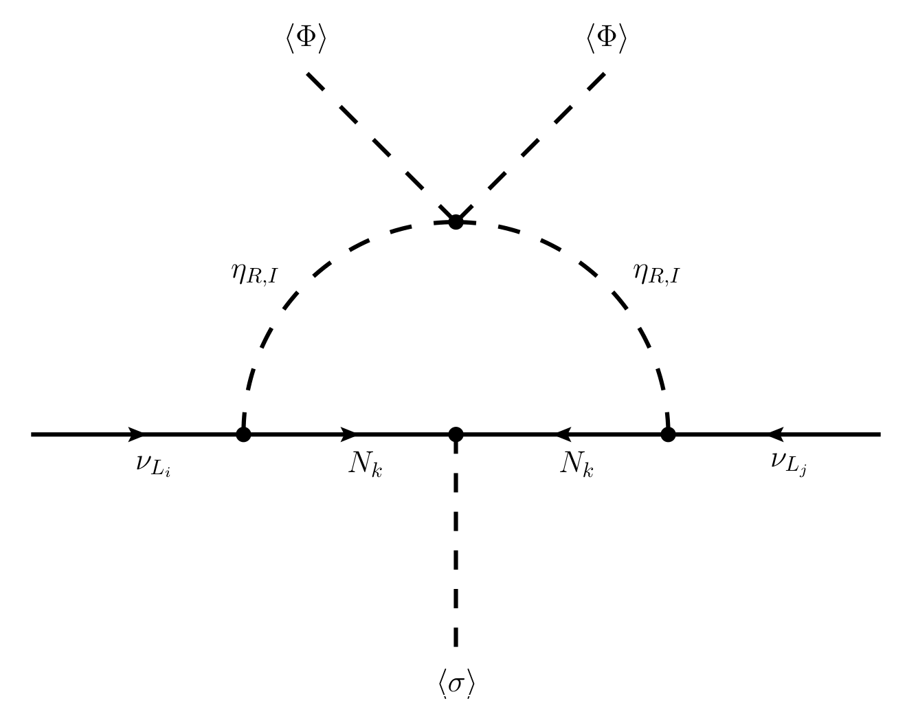
After the electroweak symmetry breaking one gets that the light neutrino mass matrix is given by the following expression Ma 2006; Babu and Ma 2008
| (13) |
III Summary of constraints
Before analysing the sensitivities of the experimental searches for WIMPs, we first discuss the theoretical and experimental restrictions that are implemented in our analysis.
III.1 Boundedness conditions
In order to ensure that the theory is perturbative the quartic couplings in the scalar potential, eq. (4), as well as the Yukawa couplings in eq. (2) are limited to be Lindner et al. 2016,
| (14) |
Furthermore, the consistency requirements of the scalar potential demand that the dimensionless parameters in eq. (4) have to fulfill the following conditions Kadastik et al. 2009,
| (15) |
From the last relations it is guaranteed that the scalar potential is bounded from below.
III.2 Searches of new physics
As we described in the previous section, there are 6 physical scalars in the model: three CP-even () and ; two CP-odd and the Majoron ; and a charged scalar . Therefore, one has to impose the constraints on the scalar masses coming from the LEP results Heister et al. 2002 and the latest reports from the LHC on the Higgs properties Tanabashi et al. 2018. Notice that the invisible Higgs decay channel is always present, namely the Higgs decay into Majorons , where in our case the SM Higgs will be identified with either or . Then, this decay mode coexists with the Higgs decay into the fermion dark matter, , when it is kinematically allowed, i.e. when . Therefore, we consider Tanabashi et al. 2018
| (16) |
On the other hand, the LEP collaboration studies on the invisible decays of and gauge bosons Heister et al. 2002 provide bounds on the masses of the inert scalars and . From these searches, the following conditions must be fulfilled Lundstrom et al. 2009
| (17) |
The LEP reports also established disallowed mass regions for the mass splitting given by,
| (18) |
and GeV.
Finally, it is important to mention that the oblique parameters , and are also sensitive to new physics Peskin and Takeuchi 1990; Peskin and Takeuchi 1992. Then, it has to be considered that values of these parameters in the model lie within the following regions Tanabashi et al. 2018.
| (19) |
III.3 Dark matter searches
The abundance of DM in the Universe, given in terms of the cosmological abundance parameter, eq. (1), provides restrictions on the parameter space of DM models. Furthermore, there exist constraints coming from searches of DM by experiments using (in)direct detection techniques. The direct dark matter detection experiments have set bounds, for DM masses above 6 GeV, on the dark matter-nucleon spin-independent scattering cross section. The most stringent bounds are set by the XENON1T experiment, that is for a DM mass of 30 GeV at 90% C.L Aprile et al. 2018. On the other hand, the astronomical gamma ray observations constrain the velocity averaged cross section of dark matter annihilation into gamma rays . The Fermi-LAT satellite has performed this indirect DM search and constraint the cross section to be Ackermann et al. 2013. Notice that there are promising searches using neutrino telescopes like IceCube Halzen and Klein 2010, Antares Ageron et al. 2011, and KM3Net Adrian-Martinez et al. 2016. Limits on the annihilation cross section for the typical WIMP mass range are not as competitive as other limits obtained with other astroparticle messengers. In additon, neutrinos are used to set bounds on spin-dependent direct dectection cross section infered from the capture and annihilation of DM in the Sun Aartsen et al. 2016; Bhattacharya et al. 2019. The tightest limits are at GeV with ..
III.4 Neutrino oscillation parameters
The neutrino masses are obtained after diagonalisation of the mass matrix given in eq. (13). The relation between and the diagonal mass matrix is given by,
| (20) |
where are the neutrino masses. Here we are not assuming a flavor-diagonal mass matrix for chaged leptons. Therefore, the lepton mixing matrix is difined as , where are the mixing angles and corresponds to the Dirac CP-violating phase. and are the matrices that diagonalise the neutrino and charged lepton square mass matrices and respectively. The lepton mixing angles are determined by neutrino oscillation experiments. From global fits of neutrino oscillation parameters de Salas et al. 2018 (for other fits of neutrino oscillation parameters we refer the reader to Capozzi et al. 2016; Esteban et al. 2019) the best fit values and the intervals for a normal neutrino mass ordering (NO) are
| (21) |
IV Numerical analysis
We have mentioned that the nature of the DM candidate in this model could be either
fermionic or scalar. This is the lightest particle with odd charge under the symmetry
and running in the neutrino mass generation loop as shown in Fig. 1.
In our study we will focus in the case in which the DM is the lightest Majorana particle 11 1 In Ref. Toma and Vicente 2014; Vicente and Yaguna 2015; Ibarra et al. 2016 has bee analyzed the situation where the DM is the Majorana fermion within the simplest scotogenic model. Note that the case in which the DM is the neutral component of the inert doublet is similar to the studies for inert doublet model Belyaev et al. 2018., i.e. . Therefore, in this case the DM annihilates via the t- and s-channel In Fig. 2 . The former is mediated by a Majorana fermion and by the inert scalars. It has been shown that the bounds on lepton flavor violation (LFV) processes, e.g. , demand small neutrino Yukawas (namely, ) and hence the t-channel mediated by the inert scalars becomes suppressed inducing DM overabundance Toma and Vicente 2014; Vicente and Yaguna 2015. However, we show that we can keep suppressed the inert scalar mediated t-channel and thanks to the s-channel mediated by the singlet it is possible to account for the right amount of DM relic abundance. As a result, it is crucial to have a non-vanishing mixing angle between CP-even parts of the Higgs doublet and the iso-singlet , eq. (7), and in agreement with current experimental data.


For the numerical analysis we have used the MicrOMEGAS Belanger et al. 2002 and performed a scan over all free parameters of the model. For the dimensionless parameters in the scalar sector we took the following intervals:
| (22) |
and being determined by the SM Higgs mass. We are taking as the SM Higgs then GeV. On the other hand, we are varying the mass of within the range GeV. Notice that we are taking masses below 125 GeV which is in perfect agreement with both the LHC and LEP constraints as long as the doublet-singlet mixing given by in eq. (7) is less than 20% Bonilla et al. 2015.
For the masses of the inert scalars we considered the following ranges,
| (23) |
and mass of the CP-odd part is determined by using the relation . For the lepton number breaking scale, namely the singlet’s vev , we have used . Bear in mind that this vev provides the mass of the heavy Majorana fermions, , whose masses (taken to be diagonal) are varied in the following ranges,
| (24) |
Since 22
2
There are regions of the parameter space for GeV but those are below the neutrino floor. is the DM candidate of the theory we have to impose
33
3
We discard contributions to the DM abundance
produced by co-annihilation processes, i.e. .
.
The above considerations are made in such a way that they all satisfy the theoretical and experimental
constraints described in Sec. III. We computed the value of the and parameters
using the expressions given in Grimus et al. 2008a; Grimus et al. 2008b, taking Tanabashi et al. 2018 and keeping
those solutions that are in agreement with the bounds given in eq. (19). It is worth to mention that
we considered only S and T within the level shown in Fig. (10.6) from reference Tanabashi et al. 2018.
In addition, we calculated the light neutrino masses feeding the neutrino mass expression given in
eq. (13) and assumed normal ordering for neutrino masses 44
4
For simplicity, we have assumed
that the Yukawa matrices and are real and diagonal. Following this assumption, the Yukawa matrix for charge
lepton is non-diagonal (such that, ) in order to fit neutrino
oscillation experimental data in eq. (20).. Then,
we took as valid only the points that satisfy the best fit values from the
global fit of neutrino oscillation parameters55
5
The sum of neutrino masses was restricted
using the cosmological limit provided by Planck, namely eV Vagnozzi et al. 2017; Aghanim et al. 2018. de Salas et al. 2018.
Our last requirement is that the annihilation cross section of the fermion DM candidate
into Majorons (see Fig. 2) is subdominant at the moment of the freeze-out in order to guarantee detectability in DM direct detection experiments and to avoid direct detection cross sections in regions far below the neutrino floor.
IV.1 Viable dark matter mass regions
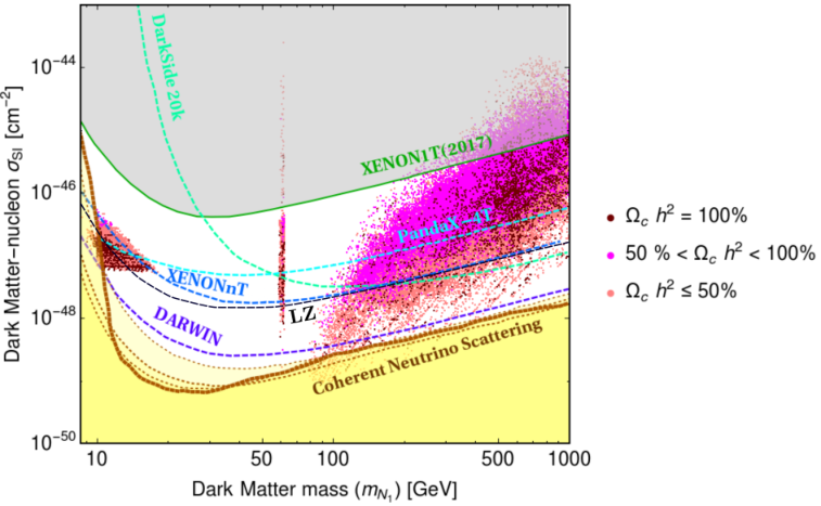
Following the considerations that we stated previously, we show in Fig. 3 the nucleon-dark matter spin-independent cross section as a function of the fermion DM mass, . From the numerical analysis we have found three different viable mass regions for a fermion DM candidate within the model. We refer as viable to those solutions that fulfil the theoretical and experimental bounds given in Section III. These are:
- •
the low mass region, with an approximate DM mass range and as dominant annihilation channel;
- •
the resonant region, where (with ); and
- •
the high mass region, for DM masses above 80 GeV where the fermion DM annihilates efficiently into the gauge bosons, i.e. with .
In all these domains, the DM annihilation into Majorons at the moment of the freeze-out is always below 10%. The latest bound coming from direct detection searches of dark matter particles is set the XENON1T experiment Aprile et al. 2018 and is defined by the top shaded area in Fig. 3. The dark red points showed in the plane account for 100% of the DM relic abundance while the solutions in purple and pink correspond only to a fraction of the DM abundance. Notice that in the high mass region it is most likely a fermion DM with a mass around 500 GeV accounting for the whole amount of DM in the Universe. There are few points around GeV and GeV that could not be distinguished from the neutrino floor background (bottom shaded area). Fig. 3 also displays the future sensitivities for dark matter searches in direct detection experiments such as XENONnT Aprile et al. 2016 and LUX-ZEPLIN Akerib et al. 2018, DarkSide-20k Aalseth et al. 2018, DARWIN Aalbers et al. 2016, and PandaX-4T Zhang et al. 2019. For completeness we provide three benchmarks in Appendix A within each mass neighbourhood and their corresponding outputs.
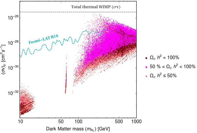
Fig. 4 shows the predictions for the velocity averaged cross section of dark matter annihilation into gamma rays as function of dark matter mass . We have found that the annihilation cross section of dark matter into gamma rays is up to two orders magnitude below the limit set by Fermi-LAT satellite results Ackermann et al. 2013 on the indirect DM search (cyan dashed line in Fig. 4). This is the case for fermion DM with a mass inside the low mass region. One can see that there are solutions in the high mass region that are ruled out by observations. In particular, the indirect search of DM excludes some points where the fermion DM represent only a fraction of the DM relic abundance. As before, all points satisfy the theoretical and experimental constraints listed in Section III and the dark red points correspond to the solutions that account for the whole amount of DM in the Universe. The lighter (purple and pink) colors would require the existence of other DM candidates to explain observations, eq. (1).
V Conclusions
In this work we have studied the scotogenic model with spontaneous breaking of lepton number. We have shown that it is possible to account for the whole amount of DM relic density thanks to the scalar singlet used to break lepton number which mixes with the CP-even part of the SM Higgs doublet. Notice that this DM annihilation portal is absent in the simplest version of the scotogenic model, where lepton number is explicitly broken by the Majorana mass term, . In our analysis the LFV processes are suppressed because the neutrino Yukawas are kept small, then experimental constraints are naturally respected. We present a numerical analysis of the parameter space of the model and the predictions for the nucleon-dark matter spin-independent cross section . We show that there are three different DM mass regions that can explain the DM relic abundance, satisfy current experimental constraints as well as the limits on reported XENON1T. We also included the future sensitivities of experiments that are devoted to search for the direct dark matter detection.
Acknowledgements.
We would like to thank A. Vicente and one of the referees for pointing out a missing factor in eq. 13. The work of C.B. was supported by the Collaborative Research Center SFB1258. R.L. was supported by Universidad Católica del Norte through the Publication Incentive program No. CPIP20180343. LMGDLV, J.M.L. and E.P. are supported by DGAPA-PAPIIT IN107118 and CONACyT CB-2017-2018/A1-S-13051 (México). C.B. would like to thank IFUNAM for the hospitality while part of this work was carried out.Appendix A Benchmarks
Here we present three benchmarks (BM1, BM2, BM3) corresponding to the different mass regions described in Section IV.1 where the fermion DM satisfy all experimental and theoretical constraints summarized in Section III, see Tables 2 and 3. Additionally, these representative points are such that the DM particle constitute 100% of the relic abundance in the Universe, see Table 4.
The values for the dimensionless parameters in the Lagrangian as well as the dimensionful parameters in the scalar potential are shown in Table 2. Notice that the neutrino Yukawas (with ) are small and as a result LFV processes are suppressed. We include as example in Table 3 the branching fractions of for each benchmark.
| [GeV] | [GeV] | [GeV] | [GeV] | [GeV] | [GeV] | [GeV] | [TeV] | [GeV2] | |
|---|---|---|---|---|---|---|---|---|---|
| BM1 | 10 | 119 | 316 | 520 | 536 | 486 | 20.7 | 10.4 | 2.1 |
| BM2 | 59.1 | 184 | 410 | 666 | 675 | 645 | 149 | 1.08 | 4.60 |
| BM3 | 707 | 924 | 940 | 1132 | 1119 | 1119 | 1498 | 5.80 | 6.98 |
| BM1 | 1.31 | 1.27 | 8.93 | -6.7 | 1.4 | -2.82 | 3.17 | 8.19 |
| BM2 | 1.57 | 1.30 | 1 | -1.4 | 1.1 | -1.99 | 9.35 | -6.76 |
| BM3 | 1.63 | 9.23 | 1.63 | 1.63 | 6.47 | -3.40 | 3.24 | -1.48 |
| BM1 | 6.78 | 8.04 | 2.14 | -1.61 | -4.99 | -4.18 |
| BM2 | 3.86 | 1.20 | 2.68 | -3.22 | -2.75 | -4.70 |
| BM3 | 8.61 | 1.12 | 1.14 | -6.33 | -8.88 | -3.17 |
| BR() | BR() | [MeV] | ||
|---|---|---|---|---|
| BM1 | 3.5 | 9.8 | - | 3.9 |
| BM2 | 9.7 | 9.2 | - | 4.2 |
| BM3 | 4 | 1.6 | 2.3 | 3.8 |
| BR() | S | T | |
|---|---|---|---|
| BM1 | 4.9 | 4.3 | 3.0 |
| BM2 | 6.8 | 2.7 | 3.2 |
| BM3 | 3.8 | 6.9 | 3.2 |
Finally, Table 4 shows the main DM annihilation channels in the model and prediction in the DM sector.
| BR() | BR() | BR() | BR() | |
|---|---|---|---|---|
| BM1 | 7.8 | 9.8 | - | - |
| BM2 | 5.9 | 9.9 | - | 2.34 |
| BM3 | 1.4 | 1.4 | - | 2.37 |
| ) | [pb] | |||
|---|---|---|---|---|
| BM1 | - | 9.4 | 1.7 | 1.21 |
| BM2 | 2 | 3.4 | 1.0 | 1.20 |
| BM3 | 4.7 | 2.2 | 4.5 | 1.19 |
References
- Whitehead (2016) L. H. Whitehead (MINOS), Nucl. Phys. B908, 130 (2016), arXiv:1601.05233 [hep-ex] .
- Decowski (2016) M. P. Decowski (KamLAND), Nucl. Phys. B908, 52 (2016).
- Abe et al. (2017) K. Abe et al. (T2K), Phys. Rev. Lett. 118, 151801 (2017), arXiv:1701.00432 [hep-ex] .
- de Salas et al. (2018) P. F. de Salas, D. V. Forero, C. A. Ternes, M. Tortola, and J. W. F. Valle, Phys. Lett. B782, 633 (2018), arXiv:1708.01186 [hep-ph] .
- Capozzi et al. (2016) F. Capozzi, E. Lisi, A. Marrone, D. Montanino, and A. Palazzo, Nucl. Phys. B908, 218 (2016), arXiv:1601.07777 [hep-ph] .
- Esteban et al. (2019) I. Esteban, M. C. Gonzalez-Garcia, A. Hernandez-Cabezudo, M. Maltoni, and T. Schwetz, JHEP 01, 106 (2019), arXiv:1811.05487 [hep-ph] .
- Minkowski (1977) P. Minkowski, Phys. Lett. 67B, 421 (1977).
- Yanagida (1979) T. Yanagida, Proceedings: Workshop on the Unified Theories and the Baryon Number in the Universe: Tsukuba, Japan, February 13-14, 1979, Conf. Proc. C7902131, 95 (1979).
- Mohapatra and Senjanovic (1980) R. N. Mohapatra and G. Senjanovic, Phys. Rev. Lett. 44, 912 (1980), [,231(1979)].
- Schechter and Valle (1980) J. Schechter and J. W. F. Valle, Phys. Rev. D22, 2227 (1980).
- Schechter and Valle (1982) J. Schechter and J. W. F. Valle, Phys. Rev. D25, 774 (1982).
- Foot et al. (1989) R. Foot, H. Lew, X. G. He, and G. C. Joshi, Z. Phys. C44, 441 (1989).
- Aghanim et al. (2018) N. Aghanim et al. (Planck), (2018), arXiv:1807.06209 [astro-ph.CO] .
- Ma (2006) E. Ma, Phys. Rev. D73, 077301 (2006), arXiv:hep-ph/0601225 [hep-ph] .
- Hagedorn et al. (2018) C. Hagedorn, J. Herrero-García, E. Molinaro, and M. A. Schmidt, JHEP 11, 103 (2018), arXiv:1804.04117 [hep-ph] .
- Blennow et al. (2019) M. Blennow, E. Fernandez-Martinez, A. Olivares-Del Campo, S. Pascoli, S. Rosauro-Alcaraz, and A. V. Titov, Eur. Phys. J. C79, 555 (2019), arXiv:1903.00006 [hep-ph] .
- Fileviez Pérez et al. (2019) P. Fileviez Pérez, C. Murgui, and A. D. Plascencia, Phys. Rev. D100, 035041 (2019), arXiv:1905.06344 [hep-ph] .
- Babu and Ma (2008) K. S. Babu and E. Ma, Int. J. Mod. Phys. A23, 1813 (2008), arXiv:0708.3790 [hep-ph] .
- Chikashige et al. (1981) Y. Chikashige, R. N. Mohapatra, and R. D. Peccei, Phys. Lett. 98B, 265 (1981).
- Joshipura and Rindani (1992) A. S. Joshipura and S. D. Rindani, Phys. Rev. Lett. 69, 3269 (1992).
- Romao et al. (1992) J. C. Romao, F. de Campos, and J. W. F. Valle, Phys. Lett. B292, 329 (1992), arXiv:hep-ph/9207269 [hep-ph] .
- Joshipura and Valle (1993) A. S. Joshipura and J. W. F. Valle, Nucl. Phys. B397, 105 (1993).
- Bonilla et al. (2015) C. Bonilla, J. W. F. Valle, and J. C. Romão, Phys. Rev. D91, 113015 (2015), arXiv:1502.01649 [hep-ph] .
- Kubo et al. (2006) J. Kubo, E. Ma, and D. Suematsu, Phys. Lett. B642, 18 (2006), arXiv:hep-ph/0604114 [hep-ph] .
- Aranda et al. (2019) A. Aranda, C. Bonilla, and E. Peinado, Phys. Lett. B792, 40 (2019), arXiv:1808.07727 [hep-ph] .
- Aad et al. (2015) G. Aad et al. (ATLAS, CMS), Phys. Rev. Lett. 114, 191803 (2015), arXiv:1503.07589 [hep-ex] .
- Lindner et al. (2016) M. Lindner, M. Platscher, C. E. Yaguna, and A. Merle, Phys. Rev. D94, 115027 (2016), arXiv:1608.00577 [hep-ph] .
- Kadastik et al. (2009) M. Kadastik, K. Kannike, and M. Raidal, Phys. Rev. D80, 085020 (2009), [Erratum: Phys. Rev.D81,029903(2010)], arXiv:0907.1894 [hep-ph] .
- Heister et al. (2002) A. Heister et al. (ALEPH), Phys. Lett. B543, 1 (2002), arXiv:hep-ex/0207054 [hep-ex] .
- Tanabashi et al. (2018) M. Tanabashi et al. (Particle Data Group), Phys. Rev. D98, 030001 (2018).
- Lundstrom et al. (2009) E. Lundstrom, M. Gustafsson, and J. Edsjo, Phys. Rev. D79, 035013 (2009), arXiv:0810.3924 [hep-ph] .
- Peskin and Takeuchi (1990) M. E. Peskin and T. Takeuchi, Phys. Rev. Lett. 65, 964 (1990).
- Peskin and Takeuchi (1992) M. E. Peskin and T. Takeuchi, Phys. Rev. D46, 381 (1992).
- Aprile et al. (2018) E. Aprile et al. (XENON), Phys. Rev. Lett. 121, 111302 (2018), arXiv:1805.12562 [astro-ph.CO] .
- Ackermann et al. (2013) M. Ackermann et al. (Fermi-LAT), Phys. Rev. D88, 082002 (2013), arXiv:1305.5597 [astro-ph.HE] .
- Halzen and Klein (2010) F. Halzen and S. R. Klein, Rev. Sci. Instrum. 81, 081101 (2010), arXiv:1007.1247 [astro-ph.HE] .
- Ageron et al. (2011) M. Ageron et al. (ANTARES), Nucl. Instrum. Meth. A656, 11 (2011), arXiv:1104.1607 [astro-ph.IM] .
- Adrian-Martinez et al. (2016) S. Adrian-Martinez et al. (KM3Net), J. Phys. G43, 084001 (2016), arXiv:1601.07459 [astro-ph.IM] .
- Aartsen et al. (2016) M. G. Aartsen et al. (IceCube), JCAP 1604, 022 (2016), arXiv:1601.00653 [hep-ph] .
- Bhattacharya et al. (2019) A. Bhattacharya, A. Esmaili, S. Palomares-Ruiz, and I. Sarcevic, JCAP 1905, 051 (2019), arXiv:1903.12623 [hep-ph] .
- Toma and Vicente (2014) T. Toma and A. Vicente, JHEP 01, 160 (2014), arXiv:1312.2840 [hep-ph] .
- Vicente and Yaguna (2015) A. Vicente and C. E. Yaguna, JHEP 02, 144 (2015), arXiv:1412.2545 [hep-ph] .
- Ibarra et al. (2016) A. Ibarra, C. E. Yaguna, and O. Zapata, Phys. Rev. D93, 035012 (2016), arXiv:1601.01163 [hep-ph] .
- Belyaev et al. (2018) A. Belyaev, G. Cacciapaglia, I. P. Ivanov, F. Rojas-Abatte, and M. Thomas, Phys. Rev. D97, 035011 (2018), arXiv:1612.00511 [hep-ph] .
- Belanger et al. (2002) G. Belanger, F. Boudjema, A. Pukhov, and A. Semenov, Comput. Phys. Commun. 149, 103 (2002), arXiv:hep-ph/0112278 [hep-ph] .
- Grimus et al. (2008a) W. Grimus, L. Lavoura, O. M. Ogreid, and P. Osland, J. Phys. G35, 075001 (2008a), arXiv:0711.4022 [hep-ph] .
- Grimus et al. (2008b) W. Grimus, L. Lavoura, O. M. Ogreid, and P. Osland, Nucl. Phys. B801, 81 (2008b), arXiv:0802.4353 [hep-ph] .
- Vagnozzi et al. (2017) S. Vagnozzi, E. Giusarma, O. Mena, K. Freese, M. Gerbino, S. Ho, and M. Lattanzi, Phys. Rev. D96, 123503 (2017), arXiv:1701.08172 [astro-ph.CO] .
- Aprile et al. (2016) E. Aprile et al. (XENON), JCAP 1604, 027 (2016), arXiv:1512.07501 [physics.ins-det] .
- Akerib et al. (2018) D. S. Akerib et al. (LUX-ZEPLIN), (2018), arXiv:1802.06039 [astro-ph.IM] .
- Aalseth et al. (2018) C. E. Aalseth et al., Eur. Phys. J. Plus 133, 131 (2018), arXiv:1707.08145 [physics.ins-det] .
- Aalbers et al. (2016) J. Aalbers et al. (DARWIN), JCAP 1611, 017 (2016), arXiv:1606.07001 [astro-ph.IM] .
- Zhang et al. (2019) H. Zhang et al. (PandaX), Sci. China Phys. Mech. Astron. 62, 31011 (2019), arXiv:1806.02229 [physics.ins-det] .