跳到论文正文
W Papers独立论文阅读器 arXiv:1908.04255 论文正文 计算阅读时间 · 0%
引用这篇论文根据当前论文元数据生成,正式投稿前建议核对。


License: arXiv.org perpetual non-exclusive license
arXiv:1908.04255v2 [cs.IT] 15 Sep 2020

Secure Coded Multi-Party Computation for Massive Matrix Operations This is an extended version of the paper, partially presented in IEEE Communication Theory Workshop (CTW), May 2018, and IEEE International Symposium on Information Theory (ISIT), June 2018 [1].

Hanzaleh Akbari Nodehi Affiliation: Department of Electrical Engineering, Sharif University of Technology    Mohammad Ali Maddah-Ali Affiliation: Nokia Bell Labs
Abstract

In this paper, we consider a secure multi-party computation problem (MPC), where the goal is to offload the computation of an arbitrary polynomial function of some massive private matrices (inputs) to a cluster of workers. The workers are not reliable. Some of them may collude to gain information about the input data (semi-honest workers). The system is initialized by sharing a (randomized) function of each input matrix to each server. Since the input matrices are massive, each share’s size is assumed to be at most 1/k1/k fraction of the input matrix, for some k∈ℕk\in\mathbb{N}. The objective is to minimize the number of workers needed to perform the computation task correctly, such that even if an arbitrary subset of t−1t-1 workers, for some t∈ℕt\in\mathbb{N}, collude, they cannot gain any information about the input matrices. We propose a sharing scheme, called polynomial sharing, and show that it admits basic operations such as adding and multiplication of matrices and transposing a matrix. By concatenating the procedures for basic operations, we show that any polynomial function of the input matrices can be calculated, subject to the problem constraints. We show that the proposed scheme can offer order-wise gain in terms of the number of workers needed, compared to the approaches formed by the concatenation of job splitting and conventional MPC approaches.

Index Terms: 
multi-party computation, polynomial sharing, secure computation, massive matrix computation

I Introduction

With the growing size of datasets in use cases such as machine learning and data science, it is inevitable to distribute the computation tasks to some external entities, which are not necessarily trusted. In this set-up, some of the major challenges are protecting the privacy of the data, guaranteeing the correctness of the result, and ensuring the efficiency of the computation.

The problem of processing private information on some external parties has been studied in the context of secure multi-party computation (MPC). Informally, in an MPC problem, some private data inputs are available in some source nodes, and the goal is to offload the computation of a specific function of those inputs to some parties (workers). These parties are not reliable. Some of them may collude to gain information about the private inputs (semi-honest workers) or even behave adversarially to make the result incorrect. Thus, the objective is to design a scheme, probably based on coding and randomization techniques, to ensure data privacy and correctness of the result. To ensure privacy, some MPC solutions, such as  [2, 3], rely on cryptographic hardness assumptions, while others, such as [4, 5, 6], are protected based on information-theoretic measures (See [7] for a survey on different approaches of MPC). In particular, the BGW scheme, named after its inventors, Ben-Or, Goldwasser, and Wigderson in [4], relies on Shamir secret sharing [8] to develop an information-theoretically private MPC scheme to calculate any polynomial of private inputs. Shamir secret sharing is an approach that allows us to share a secret, i.e., private input, among some parties, such that if the number of colluding nodes is less than a threshold, they cannot gain any information about the data. The BGW scheme exploits the fact that Shamir secret sharing admits basic operations such as addition and multiplication (at the cost of some communication among nodes).

There have been some efforts to improve MPC algorithms’ efficiency, but mainly focusing on the communication loads (see [9]). However, less effort has been dedicated to the cases where the input data is massive. One approach would be to split the computation to some smaller subtasks and dedicate a group of workers to execute each subtask, using conventional MPC approaches. In this paper, we argue that the idea of the concatenation of job splitting and multi-party computation could be significantly sub-optimal in terms of the number of workers needed.

In a seemingly irrelevant area, extensive efforts have been dedicated to using coding theory to improve the efficiency of distributed computing, mainly to cope with the stragglers [10, 11, 12, 13, 14, 15, 16, 17, 18, 19, 20]. The core idea is based on partitioning each input data into some smaller inputs and then encoding the smaller inputs. The workers then process those encoded inputs. The ultimate goal is to design the code such that the computation per worker node is limited to what it can handle, and also the final result can be derived from the outcomes of a subset of worker nodes. This is done for matrix to vector multiplication in [11], and matrix to matrix multiplication in [12, 13, 14, 15, 16]. In particular, in [13], the code is designed such that the results of different workers form a maximum distance separable (MDS), meaning that the final result can be recovered from any subset of servers with the minimum size. That approach has been extended to general matrix partitioning in [14, 15], and also for the cases where only an approximate result of the matrix multiplication is needed in [17, 20]. This paper aims to design efficient MPC schemes for massive inputs, exploiting the ideas developed in the context of coding for computing. Let us first review a motivating example that justifies our objective.

Example 1 (Maximum likelihood regression on private data:).

Assume that a research center wants to run a machine learning algorithm, say maximum likelihood regression, on a collection of private data sets, where each data set belongs to an organization. For example, each data set can be the salary information of a company (see [21]) or the medical records of a hospital. Those organizations want to help the research center, but do not want to reveal any information about their data sets beyond the final result. In particular, assume that there are Γ∈ℕ\Gamma\in\mathbb{N} organizations, where organization γ∈{1,2,…,Γ}\gamma\in\{1,2,\ldots,\Gamma\}, has a matrix 𝐗[γ]\mathbf{X}^{[\gamma]} and a corresponding target vector 𝐛[γ]\mathbf{b}^{[\gamma]}. The target value of each row of 𝐗[γ]\mathbf{X}^{[\gamma]} is the corresponding entry of vector 𝐛[γ]\mathbf{b}^{[\gamma]}. The research center aims to find a regression model b=𝐰T​𝐱b=\mathbf{w}^{T}\mathbf{x}, representing the relationship between each row of 𝐗\mathbf{X} and the corresponding entry of 𝐛\mathbf{b}, where

𝐗=[𝐗[1]𝐗[Γ]],𝐛=[𝐛[1]𝐛[Γ]].\displaystyle\mathbf{X}=\left[\begin{matrix}\mathbf{X}^{[1]}\\ \vdots\\ \mathbf{X}^{[\Gamma]}\end{matrix}\right],\ \mathbf{b}=\left[\begin{matrix}\mathbf{b}^{[1]}\\ \vdots\\ \mathbf{b}^{[\Gamma]}\end{matrix}\right]. (1)

Following the maximum likelihood solution for regression (see [22][Chapter 3.1.1], the center needs to calculate

𝐰=(𝐗T​𝐗)−1​𝐗T​𝐲,\displaystyle\mathbf{w}=(\mathbf{X}^{T}\mathbf{X})^{-1}\mathbf{X}^{T}\mathbf{y}, (2)

where (𝐗T​𝐗)−1≈𝐈+𝐀+…+𝐀k(\mathbf{X}^{T}\mathbf{X})^{-1}\approx\mathbf{I}+\mathbf{A}+\ldots+\mathbf{A}^{k}, for 𝐀=𝐈−𝐗T​𝐗\mathbf{A}=\mathbf{I}-\mathbf{X}^{T}\mathbf{X} and some k∈ℕk\in\mathbb{N} (assuming that the datasets are normalized such that the largest eigenvalue of 𝐀\mathbf{A} is less than one). For processing, assume that there are some servers available, where none of them has enough computing and storage resources to execute this computation alone. On top of that, at most t−1t-1, for some integer tt, of them may collude to gain information about the private data. Conventional MPC schemes, such as the BGW scheme [4], can handle computing polynomial functions of some private inputs (See [7]), but are not designed to handle scenarios where the inputs are massive matrices. In this paper, we aim to address such scenarios. ∎

In this paper we consider a system, including Γ\Gamma sources, NN workers, and one master. There is a link between each source and each worker. All of the workers are connected to each other and also are connected to the master. Each source sends a function of its data (so-called a share) to each worker. We assume that the workers have limited computation resources. As a proxy to that limit, we assume that each share’s size can be up to a certain fraction of the corresponding input size. The workers process their inputs, and in between, they may communicate with each other. After that, each worker sends a message to the master, such that the master can recover the required function of the inputs. The sharing and the computation procedures must be designed such that if any subset of t−1t-1 workers collude, for some t∈ℕt\in\mathbb{N}, they can not gain any information about the inputs. Also, the master must not gain any additional information, beyond the result, about the inputs. Motivated by recent results in coding for matrix multiplication, as an extension to Shamir secret sharing, in this paper, we propose a new sharing approach called polynomial sharing. We show that the proposed sharing approach admits basic operations such as addition, multiplication, and transposing, by developing a procedure for each of them. Finally, we prove that we can compute any polynomial function using these procedures while preserving the privacy subject to the storage limit of each worker node. We show that the number of servers needed to compute a function using this approach is order-wise less than what we need in approaches based on job splitting and the conventional BGW scheme.

The rest of the paper is organized as follows. In Section II, we formally state the problem setting. In Section III, we review some preliminaries and conventional approaches for MPC. In section IV, we state the main result. In Section V, we review some motivating examples. In Section VI, we present the polynomial sharing scheme. In Section VII, we show several procedures to perform basic operations, such as addition, multiplication, and transposing, using the proposed sharing scheme. In Section VIII, we present the algorithm to calculate general polynomials. Finally in Section IX, we present some extensions.

Notation: In this paper matrices and vectors are denoted by upper boldface letters and lower boldface letters respectively. For n1,n2∈ℤn_{1},n_{2}\in\mathbb{Z} the notation [n1,n2][n_{1},n_{2}] represents the set {n1,n1+1,…​n2}\{n_{1},n_{1}+1,\dots n_{2}\}. Also, [n][n] denotes the set {1,…,n}\{1,\dots,n\} for n∈ℕn\in\mathbb{N}. Furthermore, the cardinality of a set 𝒮\mathcal{S} is denoted by |𝒮||\mathcal{S}|. For the arbitrary field 𝔽\mathbb{F}, the notation 𝔽∗\mathbb{F}^{*} means any matrix with any possible size, with entries from 𝔽\mathbb{F}. For a matrix 𝐀\mathbf{A}, 𝐀(a:b,:)\mathbf{A}(a:b,:) denotes a matrix including rows aa to bb of matrix 𝐀\mathbf{A}.

I-A Concurrent and Follow-up Results

The early version of this paper was submitted to IEEE ISIT 2018 in Jan. 2018, which has been appeared in June 2018 [1]. In addition, it was presented in CTW 2018 in May 2018. We have also presented a generalized version of [1] in [23].

In parallel in [19] and [24], the authors introduce Lagrange coded computing, targeting the case where the computation of interest can be decomposed into computing one polynomial function for several (private) inputs. In other words, the computing task can be stated as computing 𝐆~​(𝐗[1]),𝐆~​(𝐗[2]),…,𝐆~​(𝐗[Γ])\tilde{\mathbf{G}}(\mathbf{X}^{[1]}),\tilde{\mathbf{G}}(\mathbf{X}^{[2]}),\dots,\tilde{\mathbf{G}}(\mathbf{X}^{[\Gamma]}) for an arbitrary polynomial function 𝐆~(.)\tilde{\mathbf{G}}(.), and inputs 𝐗[1],𝐗[2]​…,𝐗[Γ]\mathbf{X}^{[1]},\mathbf{X}^{[2]}\dots,\mathbf{X}^{[\Gamma]}. The decomposition must be such that one worker can handle one computing of 𝐆~(.)\tilde{\mathbf{G}}(.) for an input. The idea is then to use coding over those computations to form coded redundancy to deal with stragglers and/or guarantee privacy.

The major difference between [19], [24], and what we do in this paper is that in [19] and [24], one server can handle computing 𝐆~​(𝐗[γ])\tilde{\mathbf{G}}(\mathbf{X}^{[\gamma]}), for the input 𝐗[γ]\mathbf{X}^{[\gamma]}, γ∈[Γ]\gamma\in[\Gamma]. However, in this work, the objective is to compute 𝐆⁡(𝐗[1],𝐗[2]​…,𝐗[Γ])\mathbf{G}(\mathbf{X}^{[1]},\mathbf{X}^{[2]}\dots,\mathbf{X}^{[\Gamma]}), for an arbitrary polynomial 𝐆\mathbf{G}, where one server cannot handle computing 𝐆⁡(𝐗[1],𝐗[2]​…,𝐗[Γ])\mathbf{G}(\mathbf{X}^{[1]},\mathbf{X}^{[2]}\dots,\mathbf{X}^{[\Gamma]}) alone. It is clear that for an arbitrary polynomial function 𝐆⁡(𝐗[1],𝐗[2]​…,𝐗[Γ])\mathbf{G}(\mathbf{X}^{[1]},\mathbf{X}^{[2]}\dots,\mathbf{X}^{[\Gamma]}), we cannot always transform it into computing some independent calculations 𝐆~​(𝐗[1]),𝐆~​(𝐗[2])​…,𝐆~​(𝐗[Γ])\tilde{\mathbf{G}}(\mathbf{X}^{[1]}),\tilde{\mathbf{G}}(\mathbf{X}^{[2]})\dots,\tilde{\mathbf{G}}(\mathbf{X}^{[\Gamma]}) (see Example 1).

Another difference is that in [19] and [24], there is no communication among the workers and the number of workers needed for coding to be effective, is at least (Γ−1)​deg⁡(𝐆~)+1(\Gamma-1)\deg(\tilde{\mathbf{G}})+1. However, in the scheme that we propose in this paper, there is communication among the workers and the number of servers needed does not grow with Γ\Gamma or the degree of 𝐆\mathbf{G}.

The idea of [19] and [24] has been used to train some machine learning algorithms [25], in which the computation can be decomposed into calculating one specific function for several inputs. To avoid requiring too many workers, in  [25], it is suggested to approximate the specific function to a low degree polynomial function.

Another related line of research, started by [26], published in June 2018 on arXiv, is known as secure matrix multiplication. In that set-up, the objective is to calculate the multiplication of two matrices without leaking information to the workers. The scheme of [26] was later improved by the follow-up results [27, 28]. The difference between what we do in this paper and secure matrix multiplication [26, 27, 28] is that we are interested in the result of a general polynomial function of multiple private inputs, while in secure matrix multiplication, the master is interested in the result of multiplication of two matrices. Also, there is no privacy constraint for the master at the secure matrix multiplication, and there is no communication between the workers. Still, we can consider the problem of secure matrix multiplication as a special case of the proposed scenario in this paper, ignoring the extra privacy constraint that we have at the master. Indeed, the scheme that we had already proposed in [1] outperforms the scheme of the concurrent work [26] and the follow-up work [27]. The other follow-up paper [28] reports two schemes, named as GAPS-Big and GAPS-Small. Indeed, GAPS-Big is the same as what we had already reported in [1]. The scheme GAPS-Small performs better than what we report in this paper for the case of 3≤t<k3\leq t<k.

Some recent result [29] on secure matrix multiplications focuses on calculating pairwise multiplications of several pairs of matrices, rather than just one pair. This will reduce the cost of randomization per pair of multiplication (using ideas such as cross-subspace alignment) and improve the efficiency [29]. [30] considers private matrix multiplications where workers do not collude, but still the master wants to keep the input matrices private from each worker. [30] also considers the case where one of the matrices is selected from a finite and known set, and the objective is to keep the index of that matrix private. In [31], the authors propose a code for private matrix multiplication that is flexible to achieve a trade-off between the number of workers needed and the communication load. They also consider the case where one of the matrices is selected from a finite and publicity known set of matrices. A different approach to privacy in computing is introduced in [32, 33], where the function of interest is formed by a specific concatenation and combination of several known linear functions, represented by matrix operations, and the objective is to keep the order of concatenation/combination private.

II Problem Setting

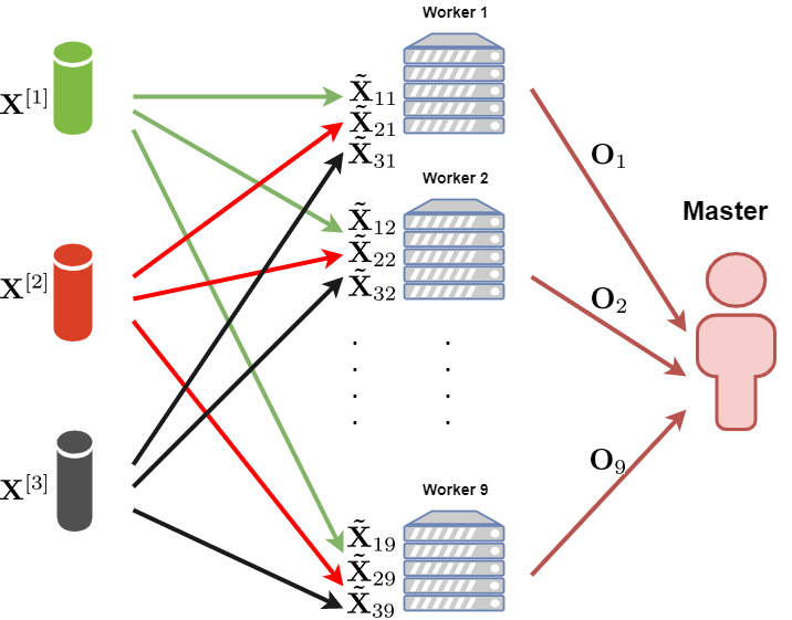
Consider an MPC system including Γ\Gamma source nodes, NN worker nodes, and one master node, for some Γ,N∈ℕ\Gamma,N\in\mathbb{N} (see Fig. 1).

Each source is connected to every single worker. In addition, every pair of workers are connected to each other. However, there is no communication link between the sources. In addition, all of the workers are connected to the master. All of these links are orthogonal11 1 By orthogonal link, we mean that they do not interfere with each other. For example, they can be wired links, or if they are wireless, they communicate at different time/frequency slots., secure, and error free.

Each source γ∈[Γ]\gamma\in[\Gamma] has access to a matrix 𝐗[γ]\mathbf{X}^{[\gamma]}, chosen from an arbitrary distribution over 𝔽m×m\mathbb{F}^{m\times m} for some finite field 𝔽\mathbb{F} and m∈ℕm\in\mathbb{N}. The master aims to know the result of a function 𝐘=𝐆⁡(𝐗[1],𝐗[2]​…,𝐗[Γ])\mathbf{Y}=\mathbf{G}(\mathbf{X}^{[1]},\mathbf{X}^{[2]}\dots,\mathbf{X}^{[\Gamma]}), where 𝐆:(𝔽m×m)Γ→𝔽m×m\mathbf{G}\colon(\mathbb{F}^{m\times m})^{\Gamma}\to\mathbb{F}^{m\times m} is an arbitrary polynomial function. The system operates in three phases: (i) sharing, (ii) computation and communication, and (iii) reconstruction. The detailed description of these phases is as follows.

  1. 1.

    Sharing: In this phase, the source γ\gamma sends 𝐗~γ​n=𝐅γ→n​(𝐗γ)\mathbf{\tilde{X}}_{\gamma n}=\mathbf{F}_{\gamma\to n}(\mathbf{X}_{\gamma}) to worker nn where 𝐅γ→n:𝔽m×m→𝔽m×mk\mathbf{F}_{\gamma\to n}\colon\mathbb{F}^{m\times m}\to\mathbb{F}^{m\times\frac{m}{k}}, for some k∈ℕk\in\mathbb{N}, k|mk|m, denotes the sharing function, used at source γ∈[Γ]\gamma\in[\Gamma], to share data with worker n∈[N]n\in[N]. The number kk represents the limit on the storage size at each worker.

  2. 2.

    Computation and Communication: In this phase, the workers process what they received, and in between, they may send some messages to other workers and continue processing. We define the set ℳn→n′∈𝔽∗\mathcal{M}_{n\to n^{\prime}}\in\mathbb{F}^{*} as the set of all messages that worker nn sends to the worker n′{n^{\prime}} in this phase, for n,n′∈[N]n,n^{\prime}\in[N].

  3. 3.

    Reconstruction: In this phase, every worker sends a message to the master. More precisely, worker nn sends the message 𝐎n∈𝔽∗\mathbf{O}_{n}\in\mathbb{F}^{*} to the master.

This scheme must satisfy three constraints.

  1. 1.

    Correctness: The master must be able to recover 𝐘\mathbf{Y} from 𝐎1,𝐎2,…,𝐎N\mathbf{O}_{1},\mathbf{O}_{2},\dots,\mathbf{O}_{N}. More precisely

    H⁡(𝐘|𝐎1,𝐎2,…,𝐎N)=0,\displaystyle H(\mathbf{Y}|\mathbf{O}_{1},\mathbf{O}_{2},\dots,\mathbf{O}_{N})=0, (3)

    where HH denotes the Shannon entropy.

  2. 2.

    Privacy at the workers: Let t∈[N]t\in[N]. Any arbitrary subset of workers, including t−1t-1 workers, must not gain any information about the inputs. In particular, for any 𝒮⊂[N]\mathcal{S}\subset[N], |𝒮|≤t−1|\mathcal{S}|\leq t-1

    H(𝐗[j],j∈[Γ]|⋃n∈𝒮{ℳn′→n,n′∈[N]},𝐗~γ​n,γ∈[Γ],n∈𝒮)=H(𝐗[j],j∈[Γ]).\displaystyle H(\mathbf{X}^{[j]},j\in[\Gamma]|\bigcup_{n\in\mathcal{S}}\{\mathcal{M}_{n^{\prime}\to n},n^{\prime}\in[N]\},\mathbf{\tilde{X}}_{\gamma n},\gamma\in[\Gamma],n\in\mathcal{S})=H(\mathbf{X}^{[j]},j\in[\Gamma]). (4)

    tt is called the security threshold of the system. In other words, we assume that there are t−1t-1 semi-honest worker nodes among the workers. It means that even-though they follow the protocol and report any calculations correctly, they are curious about the input data and may collude to gain information about it. Condition (4) guarantees that those colluding servers gain no information about the private inputs.

  3. 3.

    Privacy at the master: The master must not gain any additional information about the inputs, beyond the result of the function. In other words, 𝐘\mathbf{Y} is the only new information that is revealed to the master. More precisely,

    H(𝐗[1],𝐗[2]…,𝐗[Γ]|𝐘,𝐎1,𝐎2,…,𝐎N)=H(𝐗[1],𝐗[2]…,𝐗[Γ]|𝐘).\displaystyle H(\mathbf{X}^{[1]},\mathbf{X}^{[2]}\dots,\mathbf{X}^{[\Gamma]}|\mathbf{Y},\mathbf{O}_{1},\mathbf{O}_{2},\dots,\mathbf{O}_{N})=H(\mathbf{X}^{[1]},\mathbf{X}^{[2]}\dots,\mathbf{X}^{[\Gamma]}|\mathbf{Y}). (5)
Definition 1.

For some k,t∈ℕk,t\in\mathbb{N} and polynomial function 𝐆\mathbf{G}, we define N𝐆⋆​(t,k)N_{\mathbf{G}}^{\star}(t,k) as the minimum number of workers needed to calculate 𝐆\mathbf{G}, while the correctness, privacy at the workers, and privacy at the master are satisfied.

The objective of this paper is to find an upper bound on N𝐆⋆​(t,k)N_{\mathbf{G}}^{\star}(t,k).

Refer to caption
Fig. 1: An MPC system including Γ=3\Gamma=3 private inputs 𝐗[1],𝐗[2]\mathbf{X}^{[1]},\mathbf{X}^{[2]}, and 𝐗[3]∈𝔽m×m\mathbf{X}^{[3]}\in\mathbb{F}^{m\times m}, for m∈ℕm\in\mathbb{N}, N=9N=9 workers, and a master. All communication links are secure and error free. The size of the shares given to each worker is a fraction of the size of the inputs. Input node γ\gamma sends 𝐗~γ​n∈𝔽m×mk\mathbf{\tilde{X}}_{\gamma n}\in\mathbb{F}^{m\times\frac{m}{k}} to worker nn, for some k∈ℕ,k|mk\in\mathbb{N},k|m. Workers process their inputs while interacting with each other. Finally worker nn sends 𝐎n\mathbf{O}_{n} to the master. The master aims to know the result of a function e.g., 𝐆⁡(𝐗[1],𝐗[2],𝐗[3])=(𝐗[1])T​𝐗[2]+𝐗[3]\mathbf{G}(\mathbf{X}^{[1]},\mathbf{X}^{[2]},\mathbf{X}^{[3]})=(\mathbf{X}^{[1]})^{T}\mathbf{X}^{[2]}+\mathbf{X}^{[3]}, subject to the correctness condition (3) and privacy conditions (4), (5).

III Preliminaries: k=1k=1

As described in Section II, we have four constraints: limited storage size at each worker represented by kk, the correctness of the result, and the privacy at the workers and master. If there is no storage limit at the workers, i.e., k=1k=1, the problem is reduced to a version of secure multi-party computation, which has been extensively studied in the literature. In Particular, in [4], Ben-Or, Goldwasser, and Wigderson propose a scheme referred as the BGW scheme. To be self contained, here we briefly describe the BGW scheme in several examples. As we will see having the limit of k>1k>1 will drastically change the problem.

Example 2 (The BGW scheme for addition).

Assume that we have two sources 11 and 22 with private inputs 𝐗[1]=𝐀∈𝔽m×m\mathbf{X}^{[1]}=\mathbf{A}\in\mathbb{F}^{m\times m} and 𝐗[2]=𝐁∈𝔽m×m\mathbf{X}^{[2]}=\mathbf{B}\in\mathbb{F}^{m\times m}, respectively. These sources share their inputs with the workers. There are at most t−1t-1 semi-honest adversaries among the workers, where t∈[N]t\in[N], meaning that they follow the protocol but may collude to gain information about the input data.

The BGW protocol for this problem is as follows:

  1. 1.

    Phase 1 - Sharing:

    First phase of the BGW scheme is based on Shamir secret sharing [8]. Source 11 forms the polynomial

    𝐅𝐀​(x)=𝐀+𝐀¯1​x+𝐀¯2​x2+⋯+𝐀¯t−1​xt−1,\displaystyle\mathbf{F}_{\mathbf{A}}(x)=\mathbf{A}+\mathbf{\bar{A}}_{1}x+\mathbf{\bar{A}}_{2}x^{2}+\dots+\mathbf{\bar{A}}_{t-1}x^{t-1}, (6)

    where 𝐅𝐀​(0)=𝐀\mathbf{F}_{\mathbf{A}}(0)=\mathbf{A} is the private input at source 1 and the other coefficients, 𝐀¯i\mathbf{\bar{A}}_{i}, i∈{1,2,…​t−1}i\in\{1,2,\dots t-1\}, are chosen from 𝔽m×m\mathbb{F}^{m\times m} independently and uniformly at random. Source 1 uses 𝐅𝐀​(x)\mathbf{F}_{\mathbf{A}}(x) to share 𝐀\mathbf{A} with the workers. This means that it sends 𝐅𝐀​(αn)\mathbf{F}_{\mathbf{A}}(\alpha_{n}) to worker nn, for some distinct α1,α2,…,αN∈𝔽\alpha_{1},\alpha_{2},\dots,\alpha_{N}\in\mathbb{F}.

    We note that from Lagrange interpolation rule [34], if we have tt points from 𝐅𝐀​(x)\mathbf{F}_{\mathbf{A}}(x) we can uniquely determine this polynomial [34]. Therefore, any subset of including tt workers collaboratively can reconstruct 𝐅𝐀​(0)=𝐀\mathbf{F}_{\mathbf{A}}(0)=\mathbf{A}. Intuitively, the reason is that there are tt unknown coefficients in 𝐅𝐀​(x)\mathbf{F}_{\mathbf{A}}(x) and thus, we need at least tt equations to solve for those coefficients. Also, since coefficients, i.e., 𝐀¯i,i∈{1,2,…​t−1}\mathbf{\bar{A}}_{i},i\in\{1,2,\dots t-1\}, are chosen in 𝔽m×m\mathbb{F}^{m\times m} independently and uniformly at random, then any subset of including less than tt workers cannot reconstruct 𝐀\mathbf{A} and indeed gain no information about it. For formal proof, see [8].

    This approach is called (N,t)(N,t) sharing of 𝐀\mathbf{A} (or interchangeably (N,t)(N,t) Shamir secret sharing of 𝐀\mathbf{A}) and 𝐅𝐀​(αn)\mathbf{F}_{\mathbf{A}}(\alpha_{n}) is called the share of 𝐀\mathbf{A} at worker nn.

    Similarly, source 2 forms 𝐅𝐁​(x)\mathbf{F}_{\mathbf{B}}(x) according to the following equation and shares its secrets among the workers,

    𝐅𝐁​(x)=𝐁+𝐁¯1​x+𝐁¯2​x2+⋯+𝐁¯t−1​xt−1,\displaystyle\mathbf{F}_{\mathbf{B}}(x)=\mathbf{B}+\mathbf{\bar{B}}_{1}x+\mathbf{\bar{B}}_{2}x^{2}+\dots+\mathbf{\bar{B}}_{t-1}x^{t-1}, (7)

    where 𝐅𝐁​(0)=𝐁\mathbf{F}_{\mathbf{B}}(0)=\mathbf{B} is the private input at source 2 and 𝐁¯i\mathbf{\bar{B}}_{i}, i∈{1,2,…​t−1}i\in\{1,2,\dots t-1\}, are chosen in 𝔽m×m\mathbb{F}^{m\times m} independently and uniformly at random. Source 2 sends 𝐅𝐁​(αn)\mathbf{F}_{\mathbf{B}}(\alpha_{n}) to worker nn.

  2. 2.

    Phase 2 - Computation and Communication:

    Shamir secret sharing scheme has the linearity property, which is very important. It means that if we have the shared secrets 𝐀\mathbf{A} and 𝐁\mathbf{B} using 𝐅𝐀​(x)\mathbf{F}_{\mathbf{A}}(x) and 𝐅𝐁​(x)\mathbf{F}_{\mathbf{B}}(x), respectively among NN workers, in order to share the secret p​𝐀+q​𝐁p\mathbf{A}+q\mathbf{B} among the workers, for some constants p,q∈𝔽p,q\in\mathbb{F}, we just need that worker nn locally calculates p​𝐅𝐀​(αn)+q​𝐅𝐁​(αn)p\mathbf{F}_{\mathbf{A}}(\alpha_{n})+q\mathbf{F}_{\mathbf{B}}(\alpha_{n}). This implies that the share of p​𝐀+q​𝐁p\mathbf{A}+q\mathbf{B} are available at the workers using sharing polynomial p​𝐅𝐀​(x)+q​𝐅𝐁​(x)p\mathbf{F}_{\mathbf{A}}(x)+q\mathbf{F}_{\mathbf{B}}(x). For addition, it is sufficient to choose p=q=1p=q=1. Note that in this particular example, no communication among the nodes is needed.

  3. 3.

    Phase 3 - Reconstruction:

    In this phase worker nn sends 𝐎n=𝐅𝐀​(αn)+𝐅𝐁​(αn)\mathbf{O}_{n}=\mathbf{F}_{\mathbf{A}}(\alpha_{n})+\mathbf{F}_{\mathbf{B}}(\alpha_{n}), calculated in phase two, to the master. If the master has 𝐅𝐀​(αn)+𝐅𝐁​(αn)\mathbf{F}_{\mathbf{A}}(\alpha_{n})+\mathbf{F}_{\mathbf{B}}(\alpha_{n}) for tt or more distinct αn\alpha_{n}’s, it can recover all the coefficients of degree t−1t-1 polynomial 𝐅𝐀​(x)+𝐅𝐁​(x)\mathbf{F}_{\mathbf{A}}(x)+\mathbf{F}_{\mathbf{B}}(x). In particular, it recovers 𝐘=𝐅𝐀​(0)+𝐅𝐁​(0)=𝐀+𝐁\mathbf{Y}=\mathbf{F}_{\mathbf{A}}(0)+\mathbf{F}_{\mathbf{B}}(0)=\mathbf{A}+\mathbf{B}. One can verify that both privacy constraints (4) and (5) are satisfied.

∎

Example 3 (The BGW scheme for multiplication).

Assume that we have two sources 11 and 22 with private inputs 𝐗[1]=𝐀∈𝔽m×m\mathbf{X}^{[1]}=\mathbf{A}\in\mathbb{F}^{m\times m} and 𝐗[2]=𝐁∈𝔽m×m\mathbf{X}^{[2]}=\mathbf{B}\in\mathbb{F}^{m\times m}, respectively. In addition, the master aims to know 𝐘=𝐀T​𝐁\mathbf{Y}=\mathbf{A}^{T}\mathbf{B}. There are t−1t-1 semi-honest adversaries among the NN workers.

The BGW protocol for this problem operates as follows:

  1. 1.

    Phase 1 - Sharing:

    This phase is exactly the same as the first phase of Example 2. Therefore, at the end of this phase worker nn has 𝐅𝐀​(αn)\mathbf{F}_{\mathbf{A}}(\alpha_{n}) and 𝐅𝐁​(αn)\mathbf{F}_{\mathbf{B}}(\alpha_{n}) for some distinct α1,α2,…,αN∈𝔽\alpha_{1},\alpha_{2},\dots,\alpha_{N}\in\mathbb{F}, where 𝐅𝐀​(x)\mathbf{F}_{\mathbf{A}}(x) and 𝐅𝐁​(x)\mathbf{F}_{\mathbf{B}}(x) are defined in (6) and (7), respectively.

  2. 2.

    Phase 2 - Computation and Communication:

    In this phase, worker nn calculates 𝐅𝐀T​(αn)​𝐅𝐁​(αn)\mathbf{F}^{T}_{\mathbf{A}}(\alpha_{n})\mathbf{F}_{\mathbf{B}}(\alpha_{n}), simply by multiplying its shares of 𝐀\mathbf{A} and 𝐁\mathbf{B}. Let us define the polynomial 𝐇⁡(x)≜𝐅𝐀T​(x)​𝐅𝐁​(x)\mathbf{H}(x)\triangleq\mathbf{F}_{\mathbf{A}}^{T}(x)\mathbf{F}_{\mathbf{B}}(x). We note that 𝐇⁡(0)=𝐀T​𝐁\mathbf{H}(0)=\mathbf{A}^{T}\mathbf{B} and deg⁡(𝐇⁡(x))=2​t−2\deg(\mathbf{H}(x))=2t-2. Therefore, by having at least 2​t−12t-1 samples of this polynomial, 𝐀T​𝐁\mathbf{A}^{T}\mathbf{B} can be solved for. Therefore, if N≥2​t−1N\geq 2t-1, and these workers send their result to the master, it can calculate 𝐀T​𝐁\mathbf{A}^{T}\mathbf{B}. However, we do not do that. For some important reasons that we explain later, in Remark (1), we prefer to first have the Shamir sharing of 𝐀T​𝐁\mathbf{A}^{T}\mathbf{B} at each node. As explained before, different workers have samples of 𝐅𝐀T​(x)​𝐅𝐁​(x)\mathbf{F}_{\mathbf{A}}^{T}(x)\mathbf{F}_{\mathbf{B}}(x), and 𝐀T​𝐁=𝐅𝐀T​(0)​𝐅𝐁​(0)\mathbf{A}^{T}\mathbf{B}=\mathbf{F}_{\mathbf{A}}^{T}(0)\mathbf{F}_{\mathbf{B}}(0). However, deg⁡(𝐅𝐀T​(x)​𝐅𝐁​(x))=2​t−2≠t−1\deg(\mathbf{F}_{\mathbf{A}}^{T}(x)\mathbf{F}_{\mathbf{B}}(x))=2t-2\neq t-1. In addition, the coefficients of 𝐅𝐀T​(x)​𝐅𝐁​(x)\mathbf{F}_{\mathbf{A}}^{T}(x)\mathbf{F}_{\mathbf{B}}(x) do not have the distribution that we wish in Shamir secret sharing.

    In the BGW scheme, to have Shamir shares of 𝐀T​𝐁\mathbf{A}^{T}\mathbf{B} at each node, we use the following approach.

    We note that from Lagrange interpolation rule [34], if N≥2​t−1N\geq 2t-1, there exists a vector 𝐫=(r1,r2,…,rN)∈𝔽N\mathbf{r}=(r_{1},r_{2},\dots,r_{N})\in\mathbb{F}^{N} such that

    𝐇⁡(0)=𝐀T​𝐁=∑n=1Nrn​𝐇​(αn).\displaystyle\mathbf{H}(0)=\mathbf{A}^{T}\mathbf{B}=\sum_{n=1}^{N}r_{n}\mathbf{H}(\alpha_{n}). (8)

    In this approach, worker nn shares 𝐇⁡(αn)=𝐅𝐀T​(αn)​𝐅𝐁​(αn)\mathbf{H}(\alpha_{n})=\mathbf{F}^{T}_{\mathbf{A}}(\alpha_{n})\mathbf{F}_{\mathbf{B}}(\alpha_{n}) with other workers using Shamir secret sharing. In other words, worker nn forms a polynomial of degree t−1t-1,

    𝐅n​(x)=𝐇⁡(αn)+𝐇¯1(n)​x+𝐇¯2(n)​x2+⋯+𝐇¯t−1(n)​xt−1,\displaystyle\mathbf{F}_{n}(x)=\mathbf{H}(\alpha_{n})+\mathbf{\bar{H}}_{1}^{(n)}x+\mathbf{\bar{H}}_{2}^{(n)}x^{2}+\dots+\mathbf{\bar{H}}_{t-1}^{(n)}x^{t-1},

    where 𝐇¯i(n)\mathbf{\bar{H}}_{i}^{(n)}, i∈[t−1]i\in[t-1], n∈[N]n\in[N], are chosen independently and uniformly at random in 𝔽m×m\mathbb{F}^{m\times m}. Worker nn sends the value of 𝐅n​(αn′)\mathbf{F}_{n}(\alpha_{n^{\prime}}) to worker n′{n^{\prime}}, for all n,n′∈[N]n,n^{\prime}\in[N]. Then each worker nn calculates ∑n′=1Nrn′​𝐅n′​(αn)\sum_{n^{\prime}=1}^{N}r_{n^{\prime}}\mathbf{F}_{n^{\prime}}(\alpha_{n}). We claim that the result is indeed Shamir sharing of 𝐀T​𝐁\mathbf{A}^{T}\mathbf{B}. To verify that, let us define 𝐅⁡(x)\mathbf{F}(x) as

    𝐅⁡(x)\displaystyle\mathbf{F}(x) ≜∑n′=1Nrn′​𝐅n′​(x)\displaystyle\triangleq\sum_{n^{\prime}=1}^{N}r_{n^{\prime}}\mathbf{F}_{n^{\prime}}(x)
    =∑n′=1Nrn′​𝐇​(αn′)+x​∑n′=1Nrn′​𝐇¯1(n′)+x2​∑n′=1Nrn′​𝐇¯2(n′)+⋯+xt−1​∑n′=1Nrn′​𝐇¯t−1(n′).\displaystyle=\sum_{n^{\prime}=1}^{N}r_{n^{\prime}}\mathbf{H}(\alpha_{n^{\prime}})+x\sum_{n^{\prime}=1}^{N}r_{n^{\prime}}\mathbf{\bar{H}}_{1}^{(n^{\prime})}+x^{2}\sum_{n^{\prime}=1}^{N}r_{n^{\prime}}\mathbf{\bar{H}}_{2}^{(n^{\prime})}+\dots+x^{t-1}\sum_{n^{\prime}=1}^{N}r_{n^{\prime}}\mathbf{\bar{H}}_{t-1}^{(n^{\prime})}. (9)

    Then, we have the following observations:

    1. (i)

      Due to (8), 𝐅⁡(0)=∑n′=1Nrn′​𝐇​(αn′)=𝐀T​𝐁\mathbf{F}(0)=\sum_{n^{\prime}=1}^{N}r_{n^{\prime}}\mathbf{H}(\alpha_{n^{\prime}})=\mathbf{A}^{T}\mathbf{B}.

    2. (ii)

      Worker nn has access to 𝐅⁡(αn)=∑n′=1Nrn′​𝐅n′​(αn)\mathbf{F}(\alpha_{n})=\sum_{n^{\prime}=1}^{N}r_{n^{\prime}}\mathbf{F}_{n^{\prime}}(\alpha_{n}).

    3. (iii)

      ∑n′=1Nrn′​𝐇¯i(n′)\sum_{n^{\prime}=1}^{N}r_{n^{\prime}}\mathbf{\bar{H}}_{i}^{(n^{\prime})}, i∈[t−1]i\in[t-1], are independent with uniform distribution in 𝔽m×m\mathbb{F}^{m\times m}.

    Thus, 𝐅⁡(αn)\mathbf{F}(\alpha_{n}) is indeed a Shamir share of 𝐀T​𝐁\mathbf{A}^{T}\mathbf{B}. In addition, if tt of the workers send their samples of 𝐅⁡(x)\mathbf{F}(x) to the master, it can recover 𝐅⁡(0)=𝐀T​𝐁\mathbf{F}(0)=\mathbf{A}^{T}\mathbf{B}.

  3. 3.

    Phase 3 - Reconstruction:

    Each worker nn sends 𝐅⁡(αn)\mathbf{F}(\alpha_{n}) to the master. It can recover 𝐅⁡(0)=𝐀T​𝐁\mathbf{F}(0)=\mathbf{A}^{T}\mathbf{B}, if it has 𝐅⁡(αn)\mathbf{F}(\alpha_{n}) from tt workers.

We note that the master can also recover ∑n′=1Nrn′​𝐇¯i(n′)\sum_{n^{\prime}=1}^{N}r_{n^{\prime}}\mathbf{\bar{H}}_{i}^{(n^{\prime})}, for i∈[t−1]i\in[t-1], which reveal no information about 𝐀\mathbf{A} and 𝐁\mathbf{B}. Therefore, the privacy at the master is guaranteed. In addition, whatever is shared with a worker is based on Shamir secret sharing with new random coefficients. This can be used to prove that the privacy at the workers is guaranteed.

This example shows that if the number of workers is N≥2​t−1N\geq 2t-1, the system can calculate multiplication.

∎

Remark 1:

In this remark, we explain why we prefer to have Shamir shares of 𝐀T​𝐁\mathbf{A}^{T}\mathbf{B} at the workers. The main reason is that this approach gives us great flexibility to use it iteratively and calculate any polynomial function of the inputs. Let us assume that there are three inputs 𝐀,𝐁\mathbf{A},\mathbf{B}, and 𝐂\mathbf{C}, and the goal is to calculate 𝐂T​𝐀T​𝐁\mathbf{C}^{T}\mathbf{A}^{T}\mathbf{B}. First, we use the above approach to have the Shamir shares of 𝐃=𝐀T​𝐁\mathbf{D}=\mathbf{A}^{T}\mathbf{B} at each worker and use it again to calculate 𝐂T​𝐃\mathbf{C}^{T}\mathbf{D}. Similarly, if the goal is to calculate 𝐀T​𝐁+𝐂\mathbf{A}^{T}\mathbf{B}+\mathbf{C}, we use the above scheme to have the Shamir shares of 𝐃=𝐀T​𝐁\mathbf{D}=\mathbf{A}^{T}\mathbf{B} at each node, and use the scheme of Example 2 to calculate 𝐃+𝐂\mathbf{D}+\mathbf{C}.

Another important reason is that to calculate 𝐂T​𝐀T​𝐁\mathbf{C}^{T}\mathbf{A}^{T}\mathbf{B}, still we need N=2​t−1N=2t-1 workers. Otherwise, 𝐅𝐂T​(x)​𝐅𝐀T​(x)​𝐅𝐁​(x)\mathbf{F}_{\mathbf{C}}^{T}(x)\mathbf{F}_{\mathbf{A}}^{T}(x)\mathbf{F}_{\mathbf{B}}(x) will have degree 3​(t−1)3(t-1), and thus we will need N=3​t−2N=3t-2 workers. In other words, using this approach, the number of servers needed does not grow with the number of matrix multiplication.

This approach also makes the proof of privacy simpler.

Now let us consider the scenario where there is a storage limit for each worker, i.e., k>1k>1. One approach to deal with this case is to split the job into smaller jobs and use the BGW scheme for each sub-job, as we see in the following example.

Example 4 (Concatenation of Job Splitting and the BGW, k=2k=2).

Here, we revisit Example 3, but here, we assume that k=2k=2.

We partition each matrix into two sub-matrices as follows:

𝐀=[𝐀1𝐀2],\displaystyle\mathbf{A}=\begin{bmatrix}\mathbf{A}_{1}&\mathbf{A}_{2}\end{bmatrix}, (10)
𝐁=[𝐁1𝐁2],\displaystyle\mathbf{B}=\begin{bmatrix}\mathbf{B}_{1}&\mathbf{B}_{2}\end{bmatrix}, (11)

where 𝐀i,𝐁i∈𝔽m×m2\mathbf{A}_{i},\mathbf{B}_{i}\in\mathbb{F}^{m\times\frac{m}{2}}, for i∈{1,2}i\in\{1,2\}. We note that

𝐀T​𝐁=[𝐀1T​𝐁1𝐀1T​𝐁2𝐀2T​𝐁1𝐀2T​𝐁2].\displaystyle\mathbf{A}^{T}\mathbf{B}=\begin{bmatrix}\mathbf{A}_{1}^{T}\mathbf{B}_{1}&\mathbf{A}_{1}^{T}\mathbf{B}_{2}\\ \mathbf{A}_{2}^{T}\mathbf{B}_{1}&\mathbf{A}_{2}^{T}\mathbf{B}_{2}\end{bmatrix}.

Therefore, to calculate 𝐀T​𝐁\mathbf{A}^{T}\mathbf{B}, we can use the BGW scheme with four groups of workers to calculate 𝐀iT​𝐁j,i,j∈{1,2}\mathbf{A}^{T}_{i}\mathbf{B}_{j},i,j\in\{1,2\}, each of them with at least 2​t−12t-1 workers, following Example 3. Therefore, using this scheme, we need N=4​(2​t−1)N=4(2t-1) workers.

∎

One can see that with the concatenation of job-splitting and the BGW scheme described in Example 4, the minimum number of workers needed to calculate the addition and multiplication of two matrices is N=k​tN=kt and N=k2​(2​t−1)N=k^{2}(2t-1), respectively. In this paper, we propose an algorithm which reduces the required number of workers significantly.

IV Main Results

The main result of this paper is as follows:

Theorem 1.

For any k,t∈ℕk,t\in\mathbb{N} and any polynomial function 𝐆\mathbf{G},

N𝐆⋆​(t,k)≤min⁡{2​k2+2​t−3,k2+k​t+t−2},\displaystyle N_{\mathbf{G}}^{\star}(t,k)\leq\min\{2k^{2}+2t-3,k^{2}+kt+t-2\},

where

min⁡{2​k2+2​t−3,k2+k​t+t−2}={2​k2+2​t−3if​k<tk2+k​t+t−2if​k≥t.\min\{2k^{2}+2t-3,k^{2}+kt+t-2\}=\begin{cases}2k^{2}+2t-3&\quad\text{if}~k<t\\ k^{2}+kt+t-2&\quad\text{if}~k\geq t\end{cases}.
Remark 2:

To prove Theorem 1, we propose a scheme which is based on a novel approach for sharing called polynomial sharing and some procedures to calculate basic functions such as addition and multiplication. Using these procedures iteratively, we can calculate any polynomial function.

Remark 3:

Recall that concatenation of job splitting and MPC for multiplication needs k2​(2​t−1)k^{2}(2t-1) workers. However in the proposed scheme we can do multiplication with at most min⁡{2​k2+2​t−3,k2+k​t+t−2}\min\{2k^{2}+2t-3,k^{2}+kt+t-2\} workers, which is an orderwise improvement. For example for t=200t=200 and k=16k=16, the proposed scheme needs N=909N=909 workers, while the job splitting approach needs N=102144N=102144 workers.

Remark 4:

Theorem 1 is about the cases where there is at least one matrix multiplication in the calculation of the function 𝐆\mathbf{G}. If 𝐆\mathbf{G} is a linear function of the inputs, then the proposed scheme needs k+t−1k+t-1 workers.

Remark 5:

As mentioned in the introduction, secure matrix multiplication, which has been introduced in [26], concurrently by the conference paper of this manuscript [1], focuses on calculating the multiplication of two matrices. Ignoring the privacy constraint at the master, secure matrix multiplication can be considered as a special case of our proposed problem formulation. This line of work has been followed by [27, 28] to improve its efficiency. The number of workers needed by the scheme of [26] is equal to (k+t−1)2(k+t-1)^{2}, which is outperformed by our proposed scheme (1). The number of workers needed by the follow-up paper [27] is equal to k2+t​k+t−2k^{2}+tk+t-2, which is again outperformed by the proposed scheme (1). Reference [28] reports two schemes, named as GAPS-Big and GAPS-Small. Indeed, GAPS-Big is the same as what we had already reported in [1]. The number of servers needed by GAPS-Small is smaller than what we report in this paper, for the case where 3≤t<k3\leq t<k. The results are summarized in Table I.

TABLE I: The number of workers needed for Matrix Multiplication (SMM)
Work Date Number of Workers Needed
Our Scheme (Nodehi-MaddahAli) [1] June 2018 N={2​k2+2​t−3if​k<tk2+k​t+t−2if​k≥tN=\begin{cases}2k^{2}+2t-3&\quad\text{if}\ k<t\\ k^{2}+kt+t-2&\quad\text{if}\ k\geq t\end{cases}
SMM (Chang-Tandon [26]) June 2018 N=(k+t−1)2N=(k+t-1)^{2}
SMM (Kakar et al. [27]) Oct. 2018 N=k2+t​k+t−2N=k^{2}+tk+t-2
GASP-Big (D’ Oliveira et. al.  [28]) Dec. 2018 N={2​k2+2​t−3if​k<tk2+k​t+t−2if​k≥tN=\begin{cases}2k^{2}+2t-3&\quad\text{if}\ k<t\\ k^{2}+kt+t-2&\quad\text{if}\ k\geq t\end{cases}
GASP-Small (D’ Oliveira et. al. [28]) Dec. 2018 N={k2+2​kif​ 2=t≤kk2+2​k+(t−1)2+t−4if​ 3≤t≤kk2+k​t+2​t−5−⌊t−3k⌋if​k<t≤k⁡(k−1)+22​k2+k​t+t−2​k−1if​k​(k−1)+2<tN=\begin{cases}k^{2}+2k&\quad\text{if}\ 2=t\leq k\\ k^{2}+2k+(t-1)^{2}+t-4&\quad\text{if}\ 3\leq t\leq k\\ k^{2}+kt+2t-5-\lfloor{\frac{t-3}{k}}{\rfloor}&\quad\text{if}\ k<t\leq k(k-1)+2\\ 2k^{2}+kt+t-2k-1&\quad\text{if}\ k(k-1)+2<t\end{cases}

V Motivating example

Here, we revisit Example 4 with k=2k=2 and t=4t=4 and propose a solution that needs 13 workers, as compared to 4×7=284\times 7=28 workers in the solution of Example 4.

Example 5 (The proposed Approach for k=2k=2 and t=4t=4).

In this example we explain the proposed scheme to securely calculate 𝐋=𝐀T​𝐁\mathbf{L}=\mathbf{A}^{T}\mathbf{B}.

  1. 1.

    Phase 1 - Sharing:

    Consider the following polynomial functions

    𝐅A​(x)\displaystyle\mathbf{F}_{A}(x) =𝐀1+𝐀2​x+𝐀¯3​x4+𝐀¯4​x5+𝐀¯5​x6,\displaystyle=\mathbf{A}_{1}+\mathbf{A}_{2}x+\mathbf{\bar{A}}_{3}x^{4}+\mathbf{\bar{A}}_{4}x^{5}+\mathbf{\bar{A}}_{5}x^{6},
    𝐅𝐁​(x)\displaystyle\mathbf{F}_{\mathbf{B}}(x) =𝐁1+𝐁2​x2+𝐁¯3​x4+𝐁¯4​x5+𝐁¯5​x6,\displaystyle=\mathbf{B}_{1}+\mathbf{B}_{2}x^{2}+\mathbf{\bar{B}}_{3}x^{4}+\mathbf{\bar{B}}_{4}x^{5}+\mathbf{\bar{B}}_{5}x^{6},

    where 𝐀1,𝐀2,𝐁1\mathbf{A}_{1},\mathbf{A}_{2},\mathbf{B}_{1}, and 𝐁2\mathbf{B}_{2} are defined in (10) and (11) in Example 4. In addition, 𝐀¯i,𝐁¯i\mathbf{\bar{A}}_{i},\mathbf{\bar{B}}_{i}, for i∈[3,5]i\in[3,5], are matrices chosen independently and uniformly at random in 𝔽m×m2\mathbb{F}^{m\times\frac{m}{2}}. These polynomials follow a certain pattern. More precisely, in these polynomials the coefficients of some powers of xx are zero. In 𝐅𝐀​(x)\mathbf{F}_{\mathbf{A}}(x) the coefficients of x2x^{2} and x3x^{3} are zero and in 𝐅𝐁​(x)\mathbf{F}_{\mathbf{B}}(x) the coefficients of xx and x3x^{3} are zero. We choose α1,α2,…,αN∈𝔽\alpha_{1},\alpha_{2},\dots,\alpha_{N}\in\mathbb{F}, independently and uniformly at random. Source nodes 11 and 22 share 𝐅𝐀​(αn)\mathbf{F}_{\mathbf{A}}(\alpha_{n}) and 𝐅𝐁​(αn)\mathbf{F}_{\mathbf{B}}(\alpha_{n}) with worker nn, respectively. We call this form of sharing as polynomial sharing.

  2. 2.

    Phase 2 - Computation and Communication:

    Worker nn calculates 𝐅AT​(αn)​𝐅𝐁​(αn)\mathbf{F}_{A}^{T}(\alpha_{n})\mathbf{F}_{\mathbf{B}}(\alpha_{n}). Consider the polynomial function 𝐇⁡(x)\mathbf{H}(x) of degree 1212, defined as

    𝐇⁡(x)=∑n=012𝐇𝐧​xn≜𝐅AT​(x)​𝐅𝐁​(x).\displaystyle\mathbf{H}(x)=\sum_{n=0}^{12}\mathbf{H_{n}}x^{n}\mathrel{\triangleq}\mathbf{F}_{A}^{T}(x)\mathbf{F}_{\mathbf{B}}(x). (12)

    We note that

    𝐇0=𝐀1T​𝐁1,\displaystyle\mathbf{H}_{0}=\mathbf{A}_{1}^{T}\mathbf{B}_{1},
    𝐇1=𝐀2T​𝐁1,\displaystyle\mathbf{H}_{1}=\mathbf{A}_{2}^{T}\mathbf{B}_{1},
    𝐇2=𝐀1T​𝐁2,\displaystyle\mathbf{H}_{2}=\mathbf{A}_{1}^{T}\mathbf{B}_{2},
    𝐇3=𝐀2T​𝐁2.\displaystyle\mathbf{H}_{3}=\mathbf{A}_{2}^{T}\mathbf{B}_{2}. (13)

    If the master has 𝐇⁡(αn)\mathbf{H}(\alpha_{n}) for N≥13N\geq 13 distinct αi\alpha_{i}’s, then it can calculate all the coefficients of 𝐇⁡(x)\mathbf{H}(x), including 𝐇0=𝐀1T​𝐁1\mathbf{H}_{0}=\mathbf{A}_{1}^{T}\mathbf{B}_{1}, 𝐇1=𝐀2T​𝐁1\mathbf{H}_{1}=\mathbf{A}_{2}^{T}\mathbf{B}_{1}, 𝐇2=𝐀1T​𝐁2\mathbf{H}_{2}=\mathbf{A}_{1}^{T}\mathbf{B}_{2}, and 𝐇3=𝐀2T​𝐁2\mathbf{H}_{3}=\mathbf{A}_{2}^{T}\mathbf{B}_{2}, with probability approaching to one, as |𝔽|→∞|\mathbb{F}|\rightarrow\infty. More precisely, according to Lagrange interpolation rule [34], there are some rn(i,j)r^{(i,j)}_{n}, i,j∈{1,2}i,j\in\{1,2\} and n∈[N]n\in[N], such that

    𝐀iT​𝐁j=∑n=1Nrn(i,j)​𝐇​(αn).\displaystyle\mathbf{A}_{i}^{T}\mathbf{B}_{j}=\sum_{n=1}^{N}r^{(i,j)}_{n}\mathbf{H}(\alpha_{n}). (14)
    Remark 6:

    Note that rn(i,j)r^{(i,j)}_{n}, i,j∈{1,2}i,j\in\{1,2\} and n∈[N]n\in[N] are only functions of αn\alpha_{n}, n∈[N]n\in[N], which are known by all workers.

    Similar to Example 3 and following Remark 1, in order to prepare the scene for the next stage and cast the result of the local computation in the form of the polynomial sharing, we use the following steps. Worker nn forms 𝐐(n)​(x)\mathbf{Q}^{(n)}(x), defined as

    𝐐(n)​(x)\displaystyle\mathbf{Q}^{(n)}(x) ≜[rn(1,1)​𝐇​(αn)rn(2,1)​𝐇​(αn)]+[rn(1,2)​𝐇​(αn)rn(2,2)​𝐇​(αn)]​x2\displaystyle\mathrel{\triangleq}\begin{bmatrix}r^{(1,1)}_{n}\mathbf{H}(\alpha_{n})\\ r^{(2,1)}_{n}\mathbf{H}(\alpha_{n})\end{bmatrix}+\begin{bmatrix}r^{(1,2)}_{n}\mathbf{H}(\alpha_{n})\\ r^{(2,2)}_{n}\mathbf{H}(\alpha_{n})\end{bmatrix}x^{2}
    +𝐑0(n)​x4+𝐑1(n)​x5+𝐑2(n)​x6,\displaystyle+\mathbf{R}^{(n)}_{0}x^{4}+\mathbf{R}^{(n)}_{1}x^{5}+\mathbf{R}^{(n)}_{2}x^{6}, (15)

    where 𝐑i(n),i∈{0,1,2}\mathbf{R}^{(n)}_{i},i\in\{0,1,2\}, are chosen independently and uniformly at random in 𝔽m×m2\mathbb{F}^{m\times\frac{m}{2}}. Recall that 𝐇⁡(αn),rn(1,1),rn(1,2),rn(2,1)​and​rn(2,2)\mathbf{H}(\alpha_{n}),r^{(1,1)}_{n},r^{(1,2)}_{n},r^{(2,1)}_{n}~\text{and}~r^{(2,2)}_{n} are available at worker nn. Thus, worker nn has all the information to form 𝐐(n)​(x)\mathbf{Q}^{(n)}(x). Then worker nn sends 𝐐(n)​(αn′)\mathbf{Q}^{(n)}(\alpha_{n^{\prime}}) to worker n′{n^{\prime}}, for all n′∈[N]n^{\prime}\in[N].

    Thus, worker n′n^{\prime} will have access to the matrices {𝐐(1)​(αn′),𝐐(2)​(αn′),…,𝐐(N)​(αn′)}\{\mathbf{Q}^{(1)}(\alpha_{n^{\prime}}),\mathbf{Q}^{(2)}(\alpha_{n^{\prime}}),\dots,\mathbf{Q}^{(N)}(\alpha_{n^{\prime}})\}. Then worker n′n^{\prime} calculates ∑n=113𝐐(n)​(αn′)\sum_{n=1}^{13}\mathbf{Q}^{(n)}(\alpha_{n^{\prime}}). We claim that this summation is indeed the polynomial share of the matrix 𝐀T​𝐁\mathbf{A}^{T}\mathbf{B}. To verify that, consider the polynomial function

    𝐐⁡(x)≜∑n=1N𝐐(n)​(x).\displaystyle\mathbf{Q}(x)\mathrel{\triangleq}\sum_{n=1}^{N}\mathbf{Q}^{(n)}(x). (16)

    We note that

    𝐐⁡(x)\displaystyle\mathbf{Q}(x) ≜∑n=1N𝐐(n)​(x)\displaystyle\mathrel{\triangleq}\sum_{n=1}^{N}\mathbf{Q}^{(n)}(x)
    =∑n=1N[rn(1,1)​𝐇​(αn)rn(2,1)​𝐇​(αn)]+x2​∑n=1N[rn(1,2)​𝐇​(αn)rn(2,2)​𝐇​(αn)]+x4​∑n=1N𝐑0(n)+x5​∑n=1N𝐑1(n)+x6​∑n=1N𝐑2(n)\displaystyle=\sum_{n=1}^{N}\begin{bmatrix}r^{(1,1)}_{n}\mathbf{H}(\alpha_{n})\\ r^{(2,1)}_{n}\mathbf{H}(\alpha_{n})\end{bmatrix}+x^{2}\sum_{n=1}^{N}\begin{bmatrix}r^{(1,2)}_{n}\mathbf{H}(\alpha_{n})\\ r^{(2,2)}_{n}\mathbf{H}(\alpha_{n})\end{bmatrix}+x^{4}\sum_{n=1}^{N}\mathbf{R}^{(n)}_{0}+x^{5}\sum_{n=1}^{N}\mathbf{R}^{(n)}_{1}+x^{6}\sum_{n=1}^{N}\mathbf{R}^{(n)}_{2}
    =(a)​[𝐀1T​𝐁1𝐀2T​𝐁1]+x2​[𝐀1T​𝐁2𝐀2T​𝐁2]+x4​∑n=1N𝐑0(n)+x5​∑n=1N𝐑1(n)+x6​∑n=1N𝐑2(n)\displaystyle\overset{(a)}{=}\begin{bmatrix}\mathbf{A}_{1}^{T}\mathbf{B}_{1}\\ \mathbf{A}_{2}^{T}\mathbf{B}_{1}\end{bmatrix}+x^{2}\begin{bmatrix}\mathbf{A}_{1}^{T}\mathbf{B}_{2}\\ \mathbf{A}_{2}^{T}\mathbf{B}_{2}\end{bmatrix}+x^{4}\sum_{n=1}^{N}\mathbf{R}^{(n)}_{0}+x^{5}\sum_{n=1}^{N}\mathbf{R}^{(n)}_{1}+x^{6}\sum_{n=1}^{N}\mathbf{R}^{(n)}_{2}
    =𝐋1+𝐋2​x2+𝐋¯3​x4+𝐋¯4​x5+𝐋¯5​x6,\displaystyle=\mathbf{L}_{1}+\mathbf{L}_{2}x^{2}+\mathbf{\bar{L}}_{3}x^{4}+\mathbf{\bar{L}}_{4}x^{5}+\mathbf{\bar{L}}_{5}x^{6}, (17)

    where (a) follows from (14) and 𝐋1≜[𝐀1T​𝐁1𝐀2T​𝐁1],𝐋2≜[𝐀1T​𝐁2𝐀2T​𝐁2]\mathbf{L}_{1}\mathrel{\triangleq}\begin{bmatrix}\mathbf{A}_{1}^{T}\mathbf{B}_{1}\\ \mathbf{A}_{2}^{T}\mathbf{B}_{1}\end{bmatrix},\mathbf{L}_{2}\mathrel{\triangleq}\begin{bmatrix}\mathbf{A}_{1}^{T}\mathbf{B}_{2}\\ \mathbf{A}_{2}^{T}\mathbf{B}_{2}\end{bmatrix}, 𝐋¯3≜∑n=1N𝐑0(n)\mathbf{\bar{L}}_{3}\mathrel{\triangleq}\sum_{n=1}^{N}\mathbf{R}^{(n)}_{0}, 𝐋¯4≜∑n=1N𝐑1(n)\mathbf{\bar{L}}_{4}\mathrel{\triangleq}\sum_{n=1}^{N}\mathbf{R}^{(n)}_{1}, and 𝐋¯5≜∑n=1N𝐑2(n)\mathbf{\bar{L}}_{5}\mathrel{\triangleq}\sum_{n=1}^{N}\mathbf{R}^{(n)}_{2}. Note that, 𝐋¯i,i∈{3,4,5}\mathbf{\bar{L}}_{i},i\in\{3,4,5\}, have independent and uniform distribution in 𝔽m×m2\mathbb{F}^{m\times\frac{m}{2}}. Because of the randomness of 𝐑i(n)​(x)\mathbf{R}^{(n)}_{i}(x), for i∈{0,1,2}i\in\{0,1,2\}, n∈[N]n\in[N], and degree of 𝐐⁡(x)\mathbf{Q}(x), one can easily verify that 𝐐⁡(x)\mathbf{Q}(x) is in the form of polynomial sharing and worker nn has access to 𝐐⁡(αn)\mathbf{Q}(\alpha_{n}).

  3. 3.

    Phase3 - Reconstruction:

    Worker nn sends 𝐐⁡(αn)\mathbf{Q}(\alpha_{n}) to the master, n∈[N]n\in[N]. The master then calculates 𝐀T​𝐁\mathbf{A}^{T}\mathbf{B} from what it receives by polynomial interpolation.

∎

This algorithm guarantees conditions (4), the privacy at the workers. An intuitive explanation is that in each interaction among the workers, the algorithm uses some independent random matrices, as the coefficients of the sharing polynomials, such that any subset, including 33 workers, cannot gain any information about the input data. This will be proven formally later in Appendix B for the general cases. Also there is no information leakage at the master, as required according to the privacy constraints (5), which will be formally proven in Appendix B.

Example 6.

In this example, we aim to show how to use a new approach to securely calculate 𝐌=𝐀T​𝐁+𝐂\mathbf{M}=\mathbf{A}^{T}\mathbf{B}+\mathbf{C}, for k=2k=2 and t=4t=4.

  1. 1.

    Phase 1 - Sharing:

    Consider the following polynomial functions

    𝐅𝐀​(x)\displaystyle\mathbf{F}_{\mathbf{A}}(x) =𝐀1+𝐀2​x+𝐀¯3​x4+𝐀¯4​x5+𝐀¯5​x6,\displaystyle=\mathbf{A}_{1}+\mathbf{A}_{2}x+\mathbf{\bar{A}}_{3}x^{4}+\mathbf{\bar{A}}_{4}x^{5}+\mathbf{\bar{A}}_{5}x^{6},
    𝐅𝐁​(x)\displaystyle\mathbf{F}_{\mathbf{B}}(x) =𝐁1+𝐁2​x2+𝐁¯3​x4+𝐁4​x5+𝐁¯5​x6,\displaystyle=\mathbf{B}_{1}+\mathbf{B}_{2}x^{2}+\mathbf{\bar{B}}_{3}x^{4}+\mathbf{B}_{4}x^{5}+\mathbf{\bar{B}}_{5}x^{6},
    𝐅𝐂​(x)\displaystyle\mathbf{F}_{\mathbf{C}}(x) =𝐂1+𝐂2​x2+𝐂¯3​x4+𝐂¯4​x5+𝐂¯5​x6,\displaystyle=\mathbf{C}_{1}+\mathbf{C}_{2}x^{2}+\mathbf{\bar{C}}_{3}x^{4}+\mathbf{\bar{C}}_{4}x^{5}+\mathbf{\bar{C}}_{5}x^{6},

    where in the above equations, 𝐀1,𝐀2,𝐁1,𝐁2,𝐂1\mathbf{A}_{1},\mathbf{A}_{2},\mathbf{B}_{1},\mathbf{B}_{2},\mathbf{C}_{1}, and 𝐂2\mathbf{C}_{2} are defined similar to (10). In addition, 𝐀¯i,𝐁¯i,𝐂¯i\mathbf{\bar{A}}_{i},\mathbf{\bar{B}}_{i},\mathbf{\bar{C}}_{i}, for i∈[3,5]i\in[3,5], are matrices chosen independently and uniformly at random in 𝔽m×m2\mathbb{F}^{m\times\frac{m}{2}}. Similar to Example 5, source nodes 11, 22, and 33 share 𝐅𝐀​(αn)\mathbf{F}_{\mathbf{A}}(\alpha_{n}), 𝐅𝐁​(αn)\mathbf{F}_{\mathbf{B}}(\alpha_{n}), and 𝐅𝐂​(αn)\mathbf{F}_{\mathbf{C}}(\alpha_{n}) with worker nn.

  2. 2.

    Phase 2 - Computation and Communication: In this phase, first, all of the workers follow phase 2 of Example 5, in order to have access to 𝐐⁡(αn)\mathbf{Q}(\alpha_{n}) defined in (16), as the polynomial shares of 𝐀T​𝐁\mathbf{A}^{T}\mathbf{B}. Then each worker calculates 𝐎n=𝐐⁡(αn)+𝐅𝐂​(αn)\mathbf{O}_{n}=\mathbf{Q}(\alpha_{n})+\mathbf{F}_{\mathbf{C}}(\alpha_{n}).

  3. 3.

    Phase3 - Reconstruction:

    Worker nn sends 𝐎n\mathbf{O}_{n} to the master, n∈[N]n\in[N]. The master then calculates 𝐀T​𝐁+𝐂\mathbf{A}^{T}\mathbf{B}+\mathbf{C} from what it receives by polynomial interpolation.

∎

Remark 7:

We would like to emphasize that recasting the result of each round of computing in the form of a polynomial-sharing is a very crucial step for us and has several important advantages:

  1. 1.

    This approach gives us great flexibility to use the procedures iteratively and calculate any polynomial function of the inputs. Let us assume that there are three inputs 𝐀,𝐁\mathbf{A},\mathbf{B}, and 𝐂\mathbf{C}, and the goal is to calculate 𝐂T​𝐀T​𝐁\mathbf{C}^{T}\mathbf{A}^{T}\mathbf{B}. First, we use the multiplication procedure to have the shares of 𝐃=𝐀T​𝐁\mathbf{D}=\mathbf{A}^{T}\mathbf{B}. At the end of the multiplication procedure, the workers have the polynomial shares of 𝐃\mathbf{D} (instead of the multiplications of the shares of 𝐀\mathbf{A} and 𝐁\mathbf{B}). The workers are also given the polynomial shares of 𝐂\mathbf{C}. Thus we can use the multiplication procedure again to calculate 𝐂T​𝐃\mathbf{C}^{T}\mathbf{D}. Similarly, if the goal is to calculate 𝐀T​𝐁+𝐂\mathbf{A}^{T}\mathbf{B}+\mathbf{C} (see Example 6), we use the multiplication procedure to have the polynomial shares of 𝐃=𝐀T​𝐁\mathbf{D}=\mathbf{A}^{T}\mathbf{B} at each node, and use the addition procedure to calculate 𝐃+𝐂\mathbf{D}+\mathbf{C}.

  2. 2.

    It allows us to develop a scheme, where the number of workers needed does NOT grow with the degree of the polynomial function 𝐆(.)\mathbf{G}(.). Again assume that the goal is to calculate 𝐂T​𝐀T​𝐁\mathbf{C}^{T}\mathbf{A}^{T}\mathbf{B}. Reviewing the argument above, one can confirm that the number of workers needed to calculate 𝐂T​𝐀T​𝐁\mathbf{C}^{T}\mathbf{A}^{T}\mathbf{B} is the same as the number of workers needed to calculate 𝐀T​𝐁\mathbf{A}^{T}\mathbf{B}.

  3. 3.

    It simplifies the proof of privacy, considering the fact that we may have several rounds of computation. Reviewing the proof of privacy in Appendix B of the paper, we observe that recasting the result of each round in the form of polynomial sharing helps us develop an iterative argument and establish that the information leakage is zero. Without that, it would be very hard to prove the privacy, considering all the interaction among the workers to keep the number of workers constant.

VI Polynomial Sharing

In this section, we formally define a sharing scheme, called polynomial sharing, and in the next section, we show that it admits basic operations such as addition, multiplication of matrices, and transposing a matrix. By concatenating the procedures for basic operations, we show that any polynomial function of the input data can be calculated, subject to the problem constraints. This scheme is motivated by [13], which is a coding technique for matrix multiplication in the distributed system with stragglers.

Definition 2.

Let 𝐀∈𝔽m×m\mathbf{A}\in\mathbb{F}^{m\times m}, partitioned as

𝐀≜[𝐀1,𝐀2,…,𝐀k],\displaystyle\mathbf{A}\mathrel{\triangleq}\begin{bmatrix}\mathbf{A}_{1},&\mathbf{A}_{2},&\dots,&\mathbf{A}_{k}\end{bmatrix}, (18)

where 𝐀j∈𝔽m×mk\mathbf{A}_{j}\in\mathbb{F}^{m\times\frac{m}{k}}, for some k∈ℕk\in\mathbb{N}, k|mk|m, and j∈[k]j\in[k]. The polynomial function 𝐅𝐀,b,t,k​(x)\mathbf{F}_{\mathbf{A},b,t,k}(x), for some b∈[k]b\in[k], is defined as

𝐅𝐀,b,t,k​(x)≜∑j=1k𝐀j​xb⁡(j−1)+∑j=1t−1𝐑n​xk2+j−1,\displaystyle\mathbf{F}_{\mathbf{A},b,t,k}(x)\mathrel{\triangleq}\sum_{j=1}^{k}\mathbf{A}_{j}x^{b(j-1)}+\sum_{j=1}^{t-1}\mathbf{R}_{n}x^{k^{2}+j-1}, (19)

where 𝐀j,j=1,2,…,k\mathbf{A}_{j},j=1,2,\dots,k, are defined in (18) and 𝐑j,j=1,2,…,t−1\mathbf{R}_{j},j=1,2,\dots,t-1, are chosen independently and uniformly at random from 𝔽m×mk\mathbb{F}^{m\times\frac{m}{k}}. We say that matrix 𝐀\mathbf{A} is (b,t,k)(b,t,k) polynomial-shared with workers in [N][N], if 𝐅𝐀,b,t,k​(αn)\mathbf{F}_{\mathbf{A},b,t,k}(\alpha_{n}) is sent to worker nn, where αn∈𝔽\alpha_{n}\in\mathbb{F} are distinct constants assigned to worker nn, n∈[N]n\in[N], where k+t−1<Nk+t-1<N.

Remark 8:

Note that for b=1b=1 and k=1k=1, the polynomial sharing is reduced to Shamir secret sharing.

The following theorem about polynomial sharing will be essential in the following sections.

Theorem 2.

Let t,k,m∈ℕt,k,m\in\mathbb{N}, N≥min⁡{2​k2+2​t−3,k2+t​k+t−2}N\geq\min\{2k^{2}+2t-3,k^{2}+tk+t-2\}, k|mk|m, and 𝐀,𝐁∈𝔽m×m\mathbf{A},\mathbf{B}\in\mathbb{F}^{m\times m}. Define

𝐇⁡(x)≜𝐅𝐀,1,t,kT​(x)​𝐅𝐁,k,t,k​(x).\displaystyle\mathbf{H}(x)\mathrel{\triangleq}\mathbf{F}_{\mathbf{A},1,t,k}^{T}(x)\mathbf{F}_{\mathbf{B},k,t,k}(x).

Then for some large enough |𝔽||\mathbb{F}|, there exist distinct α1,α2,…,αN∈𝔽\alpha_{1},\alpha_{2},\dots,\alpha_{N}\in\mathbb{F}, such that for any distinct i1,i2,…,ik+t−1∈[N]i_{1},i_{2},\dots,i_{k+t-1}\in[N], we have

H⁡(𝐀|𝐅𝐀,1,t,k​(αi1),𝐅𝐀,1,t,k​(αi2),…,𝐅𝐀,1,t,k​(αik+t−1))\displaystyle H(\mathbf{A}|\mathbf{F}_{\mathbf{A},1,t,k}(\alpha_{i_{1}}),\mathbf{F}_{\mathbf{A},1,t,k}(\alpha_{i_{2}}),\dots,\mathbf{F}_{\mathbf{A},1,t,k}(\alpha_{i_{k+t-1}})) =0,\displaystyle=0, (20)
H⁡(𝐁|𝐅𝐁,k,t,k​(αi1),𝐅𝐁,k,t,k​(αi2),…,𝐅𝐁,k,t,k​(αik+t−1))\displaystyle H(\mathbf{B}|\mathbf{F}_{\mathbf{B},k,t,k}(\alpha_{i_{1}}),\mathbf{F}_{\mathbf{B},k,t,k}(\alpha_{i_{2}}),\dots,\mathbf{F}_{\mathbf{B},k,t,k}(\alpha_{i_{k+t-1}})) =0,\displaystyle=0, (21)

and

H⁡(𝐀T​𝐁|𝐇⁡(α1),𝐇⁡(α2),…,𝐇⁡(αN))=0.\displaystyle H(\mathbf{A}^{T}\mathbf{B}|\mathbf{H}(\alpha_{1}),\mathbf{H}(\alpha_{2}),\dots,\mathbf{H}(\alpha_{N}))=0. (22)

In addition, if we choose α1,α2,…,αN\alpha_{1},\alpha_{2},\dots,\alpha_{N}, independently and uniformly at random in 𝔽\mathbb{F}, the probability that (20), (21), and (22) hold, approaches to one, as |𝔽|→∞|\mathbb{F}|\rightarrow\infty.

Proof.

See Appendix A. ∎

VII Procedures

In this section, we explain several procedures to do basic operations such as addition, multiplication, and transposing, using polynomial sharing without leaking any information. By concatenating these procedures, we can calculate any polynomial function of the private input data, subject to the constraints (3), (4), and (5).

VII-A Addition

Let 𝐀,𝐁∈𝔽m×m\mathbf{A},\mathbf{B}\in\mathbb{F}^{m\times m}, and

𝐀=\displaystyle\mathbf{A}= [𝐀1,𝐀2,…,𝐀k],\displaystyle\begin{bmatrix}\mathbf{A}_{1},&\mathbf{A}_{2},&\dots,&\mathbf{A}_{k}\end{bmatrix},
𝐁=\displaystyle\mathbf{B}= [𝐁1,𝐁2,…,𝐁k],\displaystyle\begin{bmatrix}\mathbf{B}_{1},&\mathbf{B}_{2},&\dots,&\mathbf{B}_{k}\end{bmatrix},

where 𝐀i,𝐁i∈𝔽m×mk\mathbf{A}_{i},\mathbf{B}_{i}\in\mathbb{F}^{m\times\frac{m}{k}}, for i∈[k]i\in[k] and k|mk|m. In addition, assume 𝐀\mathbf{A} and 𝐁\mathbf{B} are (b,t,k)(b,t,k) polynomial-shared with workers in [N][N]. The objective is to (b,t,k)(b,t,k) polynomial-share 𝐋≜𝐀+𝐁\mathbf{L}\mathrel{\triangleq}\mathbf{A}+\mathbf{B} with workers in [N][N]. To do that we follow a one-step procedure, as follows:

  1. 1.

    Step 1- Computation:

    In this step, worker nn calculates 𝐅𝐀,b,t,k​(αn)+‌​𝐅𝐁,b,t,k​(αn)\mathbf{F}_{\mathbf{A},b,t,k}(\alpha_{n})+‌\mathbf{F}_{\mathbf{B},b,t,k}(\alpha_{n}). We claim that this summation is indeed the polynomial share of the matrix 𝐀+𝐁\mathbf{A}+\mathbf{B}. To verify that, consider the polynomial function

    𝐐⁡(x)≜𝐅𝐀,b,t,k​(x)+‌​𝐅𝐁,b,t,k​(x).\displaystyle\mathbf{Q}(x)\mathrel{\triangleq}\mathbf{F}_{\mathbf{A},b,t,k}(x)+‌\mathbf{F}_{\mathbf{B},b,t,k}(x). (23)

    We note that

    𝐐⁡(x)\displaystyle\mathbf{Q}(x) =𝐅𝐀,b,t,k​(x)+‌​𝐅𝐁,b,t,k​(x)\displaystyle=\mathbf{F}_{\mathbf{A},b,t,k}(x)+‌\mathbf{F}_{\mathbf{B},b,t,k}(x)
    =∑j=1k𝐀j​xb⁡(j−1)+∑j=1t−1𝐑¯j​xk2+j−1+∑j=1k𝐁j​xb⁡(j−1)+∑j=1t−1𝐑^j​xk2+j−1\displaystyle=\sum_{j=1}^{k}\mathbf{A}_{j}x^{b(j-1)}+\sum_{j=1}^{t-1}\mathbf{\bar{R}}_{j}x^{k^{2}+j-1}+\sum_{j=1}^{k}\mathbf{B}_{j}x^{b(j-1)}+\sum_{j=1}^{t-1}\mathbf{\hat{R}}_{j}x^{k^{2}+j-1}
    =∑j=1k(𝐀j+𝐁j)​xb⁡(j−1)+‌​∑j=1t−1(𝐑¯j+𝐑^j)​xk2+j−1\displaystyle=\sum_{j=1}^{k}(\mathbf{A}_{j}+\mathbf{B}_{j})x^{b(j-1)}+‌\sum_{j=1}^{t-1}(\mathbf{\bar{R}}_{j}+\mathbf{\hat{R}}_{j})x^{k^{2}+j-1}
    =(a)​∑j=1k𝐋j​xb⁡(j−1)+∑j=1t−1𝐑j​xk2+j−1,\displaystyle\overset{(a)}{=}\sum_{j=1}^{k}\mathbf{L}_{j}x^{b(j-1)}+\sum_{j=1}^{t-1}\mathbf{R}_{j}x^{k^{2}+j-1}, (24)

    where (a) follows from the definitions 𝐋j≜𝐀j+𝐁j\mathbf{L}_{j}\mathrel{\triangleq}\mathbf{A}_{j}+\mathbf{B}_{j} for j∈[k]j\in[k], and 𝐑j≜𝐑¯j+𝐑^j\mathbf{R}_{j}\mathrel{\triangleq}\mathbf{\bar{R}}_{j}+\mathbf{\hat{R}}_{j}, for j∈[t−1]j\in[t-1]. We note that 𝐋=[𝐋1𝐋2…𝐋k]\mathbf{L}=\begin{bmatrix}\mathbf{L}_{1}&\mathbf{L}_{2}&\dots&\mathbf{L}_{k}\end{bmatrix}. In addition, 𝐑j,j∈[t−1]\mathbf{R}_{j},j\in[t-1], have independent and uniform distribution in 𝔽m×mk\mathbb{F}^{m\times\frac{m}{k}}. Thus, 𝐐⁡(x)\mathbf{Q}(x) is in the form of (b,t,k)(b,t,k) polynomial sharing of 𝐀+𝐁\mathbf{A}+\mathbf{B} with workers in [N][N], and worker nn has access to 𝐐⁡(αn)\mathbf{Q}(\alpha_{n}). This step is detailed in Algorithm 1.

Algorithm 1 Addition
1: Inputs: Matrices 𝐀,𝐁∈𝔽m×m\mathbf{A},\mathbf{B}\in\mathbb{F}^{m\times m} which are (b,t,k)(b,t,k) polynomial-shared with workers in [N][N].
2: Worker nn adds its shares of 𝐀\mathbf{A} and 𝐁\mathbf{B}.
3: End.

VII-B Multiplication by Constant

Let 𝐀∈𝔽m×m\mathbf{A}\in\mathbb{F}^{m\times m}, and

𝐀=\displaystyle\mathbf{A}= [𝐀1,𝐀2,…,𝐀k],\displaystyle\begin{bmatrix}\mathbf{A}_{1},&\mathbf{A}_{2},&\dots,&\mathbf{A}_{k}\end{bmatrix},

for 𝐀i∈𝔽m×mk\mathbf{A}_{i}\in\mathbb{F}^{m\times\frac{m}{k}}, i∈[k]i\in[k], and k|mk|m. In addition, assume 𝐀\mathbf{A} is (b,t,k)(b,t,k) polynomial-shared with workers in [N][N]. The objective is to (b,t,k)(b,t,k) polynomial-share 𝐋≜q​𝐀\mathbf{L}\mathrel{\triangleq}q\mathbf{A} with workers in [N][N], where qq is a constant in 𝔽\mathbb{F}. To do that, we follow a one-step procedure, as follows:

  1. 1.

    Step 1- Computation:

    In this step, worker nn calculates q​𝐅𝐀,b,t,k​(αn)q\mathbf{F}_{\mathbf{A},b,t,k}(\alpha_{n}). We claim that this multiplication is indeed the polynomial share of the matrix q​𝐀q\mathbf{A}. To verify that, consider the polynomial function

    𝐐⁡(x)≜q​𝐅𝐀,b,t,k​(x).\displaystyle\mathbf{Q}(x)\mathrel{\triangleq}q\mathbf{F}_{\mathbf{A},b,t,k}(x). (25)

    We note that

    𝐐⁡(x)\displaystyle\mathbf{Q}(x) =q​𝐅𝐀,b,t,k​(x)\displaystyle=q\mathbf{F}_{\mathbf{A},b,t,k}(x)
    =q​∑j=1k𝐀j​xb⁡(j−1)+q​∑j=1t−1𝐑¯j​xk2+j−1\displaystyle=q\sum_{j=1}^{k}\mathbf{A}_{j}x^{b(j-1)}+q\sum_{j=1}^{t-1}\mathbf{\bar{R}}_{j}x^{k^{2}+j-1}
    =∑j=1kq​𝐀j​xb⁡(j−1)+‌​∑j=1t−1q​𝐑¯j​xk2+j−1\displaystyle=\sum_{j=1}^{k}q\mathbf{A}_{j}x^{b(j-1)}+‌\sum_{j=1}^{t-1}q\mathbf{\bar{R}}_{j}x^{k^{2}+j-1}
    =(a)​∑j=1k𝐋j​xb⁡(j−1)+∑j=1t−1𝐑j​xk2+j−1,\displaystyle\overset{(a)}{=}\sum_{j=1}^{k}\mathbf{L}_{j}x^{b(j-1)}+\sum_{j=1}^{t-1}\mathbf{R}_{j}x^{k^{2}+j-1}, (26)

    where (a) follows from the definitions 𝐋j≜q​𝐀j\mathbf{L}_{j}\mathrel{\triangleq}q\mathbf{A}_{j}, for j∈[k]j\in[k], and 𝐑j≜q​𝐑¯j\mathbf{R}_{j}\mathrel{\triangleq}q\mathbf{\bar{R}}_{j}, for j∈[t−1]j\in[t-1]. We note that 𝐋=[𝐋1𝐋2…𝐋k]\mathbf{L}=\begin{bmatrix}\mathbf{L}_{1}&\mathbf{L}_{2}&\dots&\mathbf{L}_{k}\end{bmatrix}. In addition, 𝐑j,j∈[t−1]\mathbf{R}_{j},j\in[t-1], have independent and uniform distribution in 𝔽m×mk\mathbb{F}^{m\times\frac{m}{k}}. Thus, 𝐐⁡(x)\mathbf{Q}(x) is in the form of (b,t,k)(b,t,k) polynomial sharing of q​𝐀q\mathbf{A} with workers in [N][N], and worker nn has access to 𝐐⁡(αn)\mathbf{Q}(\alpha_{n}). This step is detailed in Algorithm 2.

Algorithm 2 Multiplication by Constant
1: Inputs: Matrix 𝐀∈𝔽m×m\mathbf{A}\in\mathbb{F}^{m\times m} which is (b,t,k)(b,t,k) polynomial-shared with workers in [N][N], and q∈𝔽q\in\mathbb{F}.
2: Worker nn multiplies its share of 𝐀\mathbf{A} by qq.
3: End.
Remark 9:

Polynomial sharing scheme has the linearity property. It means that if matrices 𝐀\mathbf{A} and 𝐁\mathbf{B} are (b,t,k)(b,t,k) polynomial-shared with workers in [N][N], in order to (b,t,k)(b,t,k) polynomial-share 𝐋=q​𝐀+p​𝐁\mathbf{L}=q\mathbf{A}+p\mathbf{B} with workers in [N][N], it is enough that each worker just locally calculates the same computation on its shares.

VII-C Multiplication of Two Matrices

Similar to the Shamir secrete sharing scheme, calculating the shares of the multiplication of two matrices is not as simple as calculating the addition. Workers need to do some communication. In what follows, we explain the procedure.

Let us assume that 𝐀,𝐁∈𝔽m×m\mathbf{A},\mathbf{B}\in\mathbb{F}^{m\times m}, and

𝐀=\displaystyle\mathbf{A}= [𝐀1,𝐀2,…,𝐀k],\displaystyle\begin{bmatrix}\mathbf{A}_{1},&\mathbf{A}_{2},&\dots,&\mathbf{A}_{k}\end{bmatrix},
𝐁=\displaystyle\mathbf{B}= [𝐁1,𝐁2,…,𝐁k],\displaystyle\begin{bmatrix}\mathbf{B}_{1},&\mathbf{B}_{2},&\dots,&\mathbf{B}_{k}\end{bmatrix},

where 𝐀i,𝐁i∈𝔽m×mk\mathbf{A}_{i},\mathbf{B}_{i}\in\mathbb{F}^{m\times\frac{m}{k}}, for i∈[k]i\in[k] and k|mk|m. In addition, assume 𝐀\mathbf{A} and 𝐁\mathbf{B} are (1,t,k)(1,t,k) and (k,t,k)(k,t,k) polynomial-shared with workers in [N][N], respectively. The goal is to (b,t,k)(b,t,k) polynomial-share 𝐋≜𝐀T​𝐁\mathbf{L}\mathrel{\triangleq}\mathbf{A}^{T}\mathbf{B} with workers in [N][N]. We follow three steps, including computation, communication, and aggregation.

  1. 1.

    Step 1- Computation:

    Worker nn calculates 𝐅𝐀,1,t,kT​(αn)​𝐅𝐁,k,t,k​(αn)\mathbf{F}_{\mathbf{A},1,t,k}^{T}(\alpha_{n})\mathbf{F}_{\mathbf{B},k,t,k}(\alpha_{n}).

    Consider the polynomial function 𝐇⁡(x)\mathbf{H}(x) of degree 2​(k2+t−2)2(k^{2}+t-2), defined as,

    𝐇⁡(x)=∑n=02​(k2+t−2)𝐇n​xn≜𝐅𝐀,1,t,kT​(x)​𝐅𝐁,k,t,k​(x).\displaystyle\mathbf{H}(x)=\sum_{n=0}^{2(k^{2}+t-2)}\mathbf{H}_{n}x^{n}\mathrel{\triangleq}\mathbf{F}_{\mathbf{A},1,t,k}^{T}(x)\mathbf{F}_{\mathbf{B},k,t,k}(x). (27)

    It is important to note that

    𝐇i−1+k⁡(j−1)=𝐀iT​𝐁j,\displaystyle\mathbf{H}_{i-1+k(j-1)}=\mathbf{A}^{T}_{i}\mathbf{B}_{j}, (28)

    for i,j∈[k]i,j\in[k].

    According to (22), if N≥min⁡{2​k2+2​t−3,k2+t​k+t−2}N\geq\min\{2k^{2}+2t-3,k^{2}+tk+t-2\}, then with probability approaching to one, as |𝔽|→∞|\mathbb{F}|\rightarrow\infty, we can calculate all the coefficients of 𝐇⁡(x)\mathbf{H}(x), including 𝐇i−1+k⁡(j−1)=𝐀iT​𝐁j\mathbf{H}_{i-1+k(j-1)}=\mathbf{A}^{T}_{i}\mathbf{B}_{j}, for i,j∈[k]i,j\in[k], from 𝐇⁡(αn)\mathbf{H}(\alpha_{n}), n∈[N]n\in[N]. In particular, there are some rn(i,j)r^{(i,j)}_{n}, i,j∈[k]i,j\in[k] and n∈[N]n\in[N], such that

    𝐀iT​𝐁j=∑n=1Nrn(i,j)​𝐇​(αn).\displaystyle\mathbf{A}_{i}^{T}\mathbf{B}_{j}=\sum_{n=1}^{N}r^{(i,j)}_{n}\mathbf{H}(\alpha_{n}). (29)

    Note that rn(i,j)r^{(i,j)}_{n}, i,j∈[k]i,j\in[k] and n∈[N]n\in[N] are only functions of αn\alpha_{n}, n∈[N]n\in[N], which are known by all workers. Up to now worker nn has access to 𝐇⁡(αn)\mathbf{H}(\alpha_{n}). The challenge is to find a way to change the local knowledge of the 𝐇⁡(αn)\mathbf{H}(\alpha_{n}) to (b,t,k)(b,t,k) polynomial-share of 𝐋\mathbf{L}, for each worker nn.

  2. 2.

    Step 2- Communication:

    Worker nn forms the matrix 𝐇(n)\mathbf{H}^{(n)}, defined as

    𝐇(n)≜[𝐇⁡(αn)​rn(1,1)𝐇⁡(αn)​rn(1,2)…𝐇⁡(αn)​rn(1,k)𝐇⁡(αn)​rn(2,1)𝐇⁡(αn)​rn(2,2)…𝐇⁡(αn)​rn(2,k)‌​⋮𝐇⁡(αn)​rn(k,1)𝐇⁡(αn)​rn(k,2)…𝐇⁡(αn)​rn(k,k)].\displaystyle\mathbf{H}^{(n)}\mathrel{\triangleq}\begin{bmatrix}\mathbf{H}(\alpha_{n})r^{(1,1)}_{n}&\mathbf{H}(\alpha_{n})r^{(1,2)}_{n}&\dots&\mathbf{H}(\alpha_{n})r^{(1,k)}_{n}\\ \mathbf{H}(\alpha_{n})r^{(2,1)}_{n}&\mathbf{H}(\alpha_{n})r^{(2,2)}_{n}&\dots&\mathbf{H}(\alpha_{n})r^{(2,k)}_{n}\\ \vdots&‌\vdots&\vdots&\vdots\\ \mathbf{H}(\alpha_{n})r^{(k,1)}_{n}&\mathbf{H}(\alpha_{n})r^{(k,2)}_{n}&\dots&\mathbf{H}(\alpha_{n})r^{(k,k)}_{n}\\ \end{bmatrix}. (30)

    Then worker nn, (b,t,k)(b,t,k) polynomial-shares 𝐇(n)\mathbf{H}^{(n)} with workers in [N][N]. More precisely, according to (19), worker nn forms the following polynomial,

    𝐅𝐇(n),b,t,k​(x)=∑j=1k𝐇j(n)​xb⁡(j−1)+∑j=1t−1𝐑¯j(n)​xk2+j−1,\displaystyle\mathbf{F}_{\mathbf{H}^{(n)},b,t,k}(x)=\sum_{j=1}^{k}\mathbf{H}^{(n)}_{j}x^{b(j-1)}+\sum_{j=1}^{t-1}\mathbf{\bar{R}}^{(n)}_{j}x^{k^{2}+j-1}, (31)

    where 𝐇j(n)≜[𝐇⁡(αn)​rn(1,j)𝐇⁡(αn)​rn(2,j)𝐇⁡(αn)​rn(k,j)]\mathbf{H}^{(n)}_{j}\mathrel{\triangleq}\begin{bmatrix}\mathbf{H}(\alpha_{n})r^{(1,j)}_{n}\\ \mathbf{H}(\alpha_{n})r^{(2,j)}_{n}\\ \vdots\\ \mathbf{H}(\alpha_{n})r^{(k,j)}_{n}\end{bmatrix}, for j∈[k]j\in[k] and 𝐑¯j(n),j=1,2,…,t−1\mathbf{\bar{R}}^{(n)}_{j},j=1,2,\dots,t-1, are chosen independently and uniformly at random in 𝔽m×mk\mathbb{F}^{m\times\frac{m}{k}}. Worker nn sends 𝐅𝐇(n),b,t,k​(αn′)\mathbf{F}_{\mathbf{H}^{(n)},b,t,k}(\alpha_{n^{\prime}}) to the worker n′n^{\prime}, for all n′∈[N]n^{\prime}\in[N]. All of the workers follow the same method. Thus, at the end of this step, each worker n′n^{\prime} has access to the matrices {𝐅𝐇(1),b,t,k​(αn′),𝐅𝐇(2),b,t,k​(αn′),…,𝐅𝐇(N),b,t,k​(αn′)}\{\mathbf{F}_{\mathbf{H}^{(1)},b,t,k}(\alpha_{n^{\prime}}),\mathbf{F}_{\mathbf{H}^{(2)},b,t,k}(\alpha_{n^{\prime}}),\dots,\mathbf{F}_{\mathbf{H}^{(N)},b,t,k}(\alpha_{n^{\prime}})\}.

  3. 3.

    Step 3- Aggregation:

    Now worker n′n^{\prime} calculates ∑n=1N𝐅𝐇(n),b,t,k​(αn′)\sum_{n=1}^{N}\mathbf{F}_{\mathbf{H}^{(n)},b,t,k}(\alpha_{n^{\prime}}). We claim that this summation is indeed the polynomial share of the matrix 𝐀T​𝐁\mathbf{A}^{T}\mathbf{B}. To verify that, consider the polynomial function

    𝐐⁡(x)≜∑n=1N𝐅𝐇(n),b,t,k​(x).\displaystyle\mathbf{Q}(x)\mathrel{\triangleq}\sum_{n=1}^{N}\mathbf{F}_{\mathbf{H}^{(n)},b,t,k}(x). (32)

    We note that

    𝐐⁡(x)\displaystyle\mathbf{Q}(x) =∑n=1N𝐅𝐇(n),b,t,k​(x)\displaystyle=\sum_{n=1}^{N}\mathbf{F}_{\mathbf{H}^{(n)},b,t,k}(x)
    =∑n=1N∑j=1k𝐇j(n)​xb⁡(j−1)+∑n=1N∑j=1t−1𝐑¯j(n)​xk2+j−1\displaystyle=\sum_{n=1}^{N}\sum_{j=1}^{k}\mathbf{H}^{(n)}_{j}x^{b(j-1)}+\sum_{n=1}^{N}\sum_{j=1}^{t-1}\mathbf{\bar{R}}^{(n)}_{j}x^{k^{2}+j-1}
    =∑n=1N∑j=1k[𝐇⁡(αn)​rn(1,j)𝐇⁡(αn)​rn(2,j)𝐇⁡(αn)​rn(k,j)]​xb⁡(j−1)+∑n=1N∑j=1t−1𝐑¯j(n)​xk2+j−1\displaystyle=\sum_{n=1}^{N}\sum_{j=1}^{k}\begin{bmatrix}\mathbf{H}(\alpha_{n})r^{(1,j)}_{n}\\ \mathbf{H}(\alpha_{n})r^{(2,j)}_{n}\\ \vdots\\ \mathbf{H}(\alpha_{n})r^{(k,j)}_{n}\end{bmatrix}x^{b(j-1)}+\sum_{n=1}^{N}\sum_{j=1}^{t-1}\mathbf{\bar{R}}^{(n)}_{j}x^{k^{2}+j-1}
    =∑j=1k∑n=1N[𝐇⁡(αn)​rn(1,j)𝐇⁡(αn)​rn(2,j)𝐇⁡(αn)​rn(k,j)]​xb⁡(j−1)+∑j=1t−1∑n=1N𝐑¯j(n)​xk2+j−1\displaystyle=\sum_{j=1}^{k}\sum_{n=1}^{N}\begin{bmatrix}\mathbf{H}(\alpha_{n})r^{(1,j)}_{n}\\ \mathbf{H}(\alpha_{n})r^{(2,j)}_{n}\\ \vdots\\ \mathbf{H}(\alpha_{n})r^{(k,j)}_{n}\end{bmatrix}x^{b(j-1)}+\sum_{j=1}^{t-1}\sum_{n=1}^{N}\mathbf{\bar{R}}^{(n)}_{j}x^{k^{2}+j-1}
    =(a)​∑j=1k[𝐀1T​𝐁j𝐀2T​𝐁j𝐀kT​𝐁j]​xb⁡(j−1)+‌​∑j=1t−1(∑n=1N𝐑¯j(n))​xk2+j−1=\displaystyle\overset{(a)}{=}\sum_{j=1}^{k}\begin{bmatrix}\mathbf{A}^{T}_{1}\mathbf{B}_{j}\\ \mathbf{A}^{T}_{2}\mathbf{B}_{j}\\ \vdots\\ \mathbf{A}^{T}_{k}\mathbf{B}_{j}\end{bmatrix}x^{b(j-1)}+‌\sum_{j=1}^{t-1}(\sum_{n=1}^{N}\mathbf{\bar{R}}^{(n)}_{j})x^{k^{2}+j-1}=
    =(b)​∑j=1k𝐋j​xb⁡(j−1)+𝐑j​xk2+j−1,\displaystyle\overset{(b)}{=}\sum_{j=1}^{k}\mathbf{L}_{j}x^{b(j-1)}+\mathbf{R}_{j}x^{k^{2}+j-1}, (33)

    where (a) follows from (29), and (b) follows from the definitions 𝐋j≜[𝐀1T​𝐁j𝐀2T​𝐁j𝐀kT​𝐁j]\mathbf{L}_{j}\mathrel{\triangleq}\begin{bmatrix}\mathbf{A}^{T}_{1}\mathbf{B}_{j}\\ \mathbf{A}^{T}_{2}\mathbf{B}_{j}\\ \vdots\\ \mathbf{A}^{T}_{k}\mathbf{B}_{j}\end{bmatrix}, for j∈[k]j\in[k] and 𝐑j≜∑n=1N𝐑¯j(n)\mathbf{R}_{j}\mathrel{\triangleq}\sum_{n=1}^{N}\mathbf{\bar{R}}^{(n)}_{j}, for j∈[t−1]j\in[t-1]. We note that 𝐋=[𝐋1𝐋2…𝐋k]\mathbf{L}=\begin{bmatrix}\mathbf{L}_{1}&\mathbf{L}_{2}&\dots&\mathbf{L}_{k}\end{bmatrix}. In addition, 𝐑j,j∈[t−1]\mathbf{R}_{j},j\in[t-1], have independent and uniform distribution in 𝔽m×mk\mathbb{F}^{m\times\frac{m}{k}}. Thus, 𝐐⁡(x)\mathbf{Q}(x) is in the form of (b,t,k)(b,t,k) polynomial sharing of 𝐀T​𝐁\mathbf{A}^{T}\mathbf{B} with workers in [N][N], and worker nn has access to 𝐐⁡(αn)\mathbf{Q}(\alpha_{n}). These steps are detailed in Algorithm 3.

Algorithm 3 Multiplication of Two Matrices
1: Inputs: Number NN of the workers. Matrices 𝐀\mathbf{A}, 𝐁\mathbf{B} which are (1,t,k)(1,t,k) and (k,t,k)(k,t,k) polynomial-shared with workers in [N][N], respectively. Also α1,α2,…,αN∈𝔽\alpha_{1},\alpha_{2},\dots,\alpha_{N}\in\mathbb{F}, rn(i,j)r^{(i,j)}_{n}, for i,j∈[k]i,j\in[k], and n∈[N]n\in[N] are known by all workers.
2: Step 1- Computation:
3: Worker nn calculates 𝐇⁡(αn)=Δ𝐅𝐀,1,t,kT​(αn)​𝐅𝐁,k,t,k​(αn)\mathbf{H}(\alpha_{n})\mathrel{\mathop{\kern 0.0pt=}\limits^{\Delta}}\mathbf{F}_{\mathbf{A},1,t,k}^{T}(\alpha_{n})\mathbf{F}_{\mathbf{B},k,t,k}(\alpha_{n}).
4: Step 2- Communication:
5: Worker nn, (b,t,k)(b,t,k) polynomial-shares the matrix
𝐇(n)≜[𝐇⁡(αn)​rn(1,1)𝐇⁡(αn)​rn(1,2)…𝐇⁡(αn)​rn(1,k)𝐇⁡(αn)​rn(2,1)𝐇⁡(αn)​rn(2,2)…𝐇⁡(αn)​rn(2,k)‌​⋮𝐇⁡(αn)​rn(k,1)𝐇⁡(αn)​rn(k,2)…𝐇⁡(αn)​rn(k,k)],\displaystyle\mathbf{H}^{(n)}\mathrel{\triangleq}\begin{bmatrix}\mathbf{H}(\alpha_{n})r^{(1,1)}_{n}&\mathbf{H}(\alpha_{n})r^{(1,2)}_{n}&\dots&\mathbf{H}(\alpha_{n})r^{(1,k)}_{n}\\ \mathbf{H}(\alpha_{n})r^{(2,1)}_{n}&\mathbf{H}(\alpha_{n})r^{(2,2)}_{n}&\dots&\mathbf{H}(\alpha_{n})r^{(2,k)}_{n}\\ \vdots&‌\vdots&\vdots\\ \mathbf{H}(\alpha_{n})r^{(k,1)}_{n}&\mathbf{H}(\alpha_{n})r^{(k,2)}_{n}&\dots&\mathbf{H}(\alpha_{n})r^{(k,k)}_{n}\\ \end{bmatrix},
with workers in [N][N].
6: Step 3- Aggregation:
7: Worker nn calculates the sum of the messages received in the last step.
8: End.

VII-D Transposing

Let 𝐀∈𝔽m×m\mathbf{A}\in\mathbb{F}^{m\times m}, and

𝐀=\displaystyle\mathbf{A}= [𝐀1,𝐀2,…,𝐀k],\displaystyle\begin{bmatrix}\mathbf{A}_{1},&\mathbf{A}_{2},&\dots,&\mathbf{A}_{k}\end{bmatrix},

where 𝐀i∈𝔽m×mk\mathbf{A}_{i}\in\mathbb{F}^{m\times\frac{m}{k}}, for i∈[k]i\in[k] and k|mk|m. In addition, assume 𝐀\mathbf{A} is (b,t,k)(b,t,k) polynomial-shared with workers in [N][N]. The goal is to (b,t,k)(b,t,k) polynomial-share 𝐋≜𝐀T\mathbf{L}\mathrel{\triangleq}\mathbf{A}^{T}with workers in [N][N]. We follow three steps, including splitting, communication, and aggregation.

  1. 1.

    Step 1- Splitting:

    Let us define

    𝐅i(x)≜𝐅𝐀,b,t,k(x)(mk(i−1):mki,:).\displaystyle\mathbf{F}_{i}(x)\mathrel{\triangleq}\mathbf{F}_{\mathbf{A},b,t,k}(x)(\frac{m}{k}(i-1):\frac{m}{k}i,:). (34)

    In other words, 𝐅i​(x)\mathbf{F}_{i}(x), i∈[k]i\in[k], is a sub-matrix of 𝐅𝐀,b,t,k​(x)\mathbf{F}_{\mathbf{A},b,t,k}(x), including rows from mk​(i−1)\frac{m}{k}(i-1) to mk​i\frac{m}{k}i. One can see that we have

    𝐅i​(x)=∑j=1k𝐀i​j​xb⁡(j−1)+∑j=1t−1𝐑¯i​j​xk2+j−1,\displaystyle\mathbf{F}_{i}(x)=\sum_{j=1}^{k}\mathbf{A}_{ij}x^{b(j-1)}+\sum_{j=1}^{t-1}\mathbf{\bar{R}}_{ij}x^{k^{2}+j-1}, (35)

    where

    𝐀≜[𝐀11𝐀12…‌​𝐀1​k𝐀21𝐀22…‌​𝐀2​k‌​⋮…‌​⋮𝐀k​1𝐀k​2…‌​𝐀k​k],\displaystyle\mathbf{A}\mathrel{\triangleq}\begin{bmatrix}\mathbf{A}_{11}&\mathbf{A}_{12}&\dots&‌\mathbf{A}_{1k}\\ \mathbf{A}_{21}&\mathbf{A}_{22}&\dots&‌\mathbf{A}_{2k}\\ \vdots&‌\vdots&\dots&‌\vdots\\ \mathbf{A}_{k1}&\mathbf{A}_{k2}&\dots&‌\mathbf{A}_{kk}\end{bmatrix},

    and 𝐀i​j∈𝔽mk×mk\mathbf{A}_{ij}\in\mathbb{F}^{\frac{m}{k}\times\frac{m}{k}}, for i,j∈[k]i,j\in[k] and according to (19), 𝐑¯i​j\mathbf{\bar{R}}_{ij}, for i,j∈[k]i,j\in[k], are independently and uniformly distributed in 𝔽mk×mk\mathbb{F}^{\frac{m}{k}\times\frac{m}{k}}. Since each worker nn has access to 𝐅𝐀,b,t,k​(αn)\mathbf{F}_{\mathbf{A},b,t,k}(\alpha_{n}), it has access to 𝐅i​(αn)\mathbf{F}_{i}(\alpha_{n}), too. Similar to (20) and (21), it can be proven that if N≥(k+t−1)N\geq(k+t-1), then by having 𝐅i​(αn)\mathbf{F}_{i}(\alpha_{n}), for n=1,2,…,Nn=1,2,\dots,N, we can calculate all the coefficients of 𝐅i​(x)\mathbf{F}_{i}(x), including 𝐀i​j\mathbf{A}_{ij}, for j∈[k]j\in[k], with probability approaching to one, as |𝔽|→∞|\mathbb{F}|\rightarrow\infty. More precisely, similar to (20) and (21), it can be proven that for any distinct i1,i2,…,ik+t−1∈[N]i_{1},i_{2},\dots,i_{k+t-1}\in[N], independently and uniformly at random chosen parameters α1,α2,…,αN∈𝔽\alpha_{1},\alpha_{2},\dots,\alpha_{N}\in\mathbb{F}, and i,j∈[k]i,j\in[k], with probability approaching to one, as |𝔽|→∞|\mathbb{F}|\rightarrow\infty we have

    H⁡(𝐀i​j|𝐅i​(αi1),𝐅i​(αi2),…,𝐅i​(αik+t−1))=0.\displaystyle H(\mathbf{A}_{ij}|\mathbf{F}_{i}(\alpha_{i_{1}}),\mathbf{F}_{i}(\alpha_{i_{2}}),\dots,\mathbf{F}_{i}(\alpha_{i_{k+t-1}}))=0.

    In particular, there are some rn(j)r^{(j)}_{n}, such that for i,j∈[k]i,j\in[k], and n∈[N]n\in[N],

    𝐀i​j=∑n=1Nrn(j)​𝐅i​(αn).\displaystyle\mathbf{A}_{ij}=\sum_{n=1}^{N}r^{(j)}_{n}\mathbf{F}_{i}(\alpha_{n}). (36)

    Note that rn(j)r^{(j)}_{n}, j∈[k]j\in[k] and n∈[N]n\in[N], are only functions of αn\alpha_{n}, n∈[N]n\in[N], which are known by all workers.

  2. 2.

    Step 2- Communication:

    Worker nn forms the matrix 𝐇(n)\mathbf{H}^{(n)} defined as

    𝐇(n)≜[𝐅1​(αn)​rn(1)‌​𝐅2​(αn)​rn(1)‌​…𝐅k​(αn)​rn(1)𝐅1​(αn)​rn(2)‌​𝐅2​(αn)​rn(2)‌​…𝐅k​(αn)​rn(2)𝐅1​(αn)​rn(k)‌​𝐅2​(αn)​rn(k)‌​…𝐅k​(αn)​rn(k)].\displaystyle\mathbf{H}^{(n)}\mathrel{\triangleq}\begin{bmatrix}\mathbf{F}_{1}(\alpha_{n})r^{(1)}_{n}&‌\mathbf{F}_{2}(\alpha_{n})r^{(1)}_{n}&‌\dots&\mathbf{F}_{k}(\alpha_{n})r^{(1)}_{n}\\ \mathbf{F}_{1}(\alpha_{n})r^{(2)}_{n}&‌\mathbf{F}_{2}(\alpha_{n})r^{(2)}_{n}&‌\dots&\mathbf{F}_{k}(\alpha_{n})r^{(2)}_{n}\\ \vdots&\vdots&\vdots\\ \mathbf{F}_{1}(\alpha_{n})r^{(k)}_{n}&‌\mathbf{F}_{2}(\alpha_{n})r^{(k)}_{n}&‌\dots&\mathbf{F}_{k}(\alpha_{n})r^{(k)}_{n}\end{bmatrix}. (37)

    Then worker nn, (b,t,k)(b,t,k) polynomial-shares 𝐇(n)\mathbf{H}^{(n)} with workers in [N][N]. More precisely, according to (19), worker nn forms the following polynomial

    𝐅𝐇(n),b,t,k​(x)=∑j=1k𝐇j(n)​xb⁡(j−1)+∑j=1t−1𝐑^j(n)​xk2+j−1,\displaystyle\mathbf{F}_{\mathbf{H}^{(n)},b,t,k}(x)=\sum_{j=1}^{k}\mathbf{H}^{(n)}_{j}x^{b(j-1)}+\sum_{j=1}^{t-1}\mathbf{\hat{R}}^{(n)}_{j}x^{k^{2}+j-1}, (38)

    where 𝐇j(n)≜[𝐅j​(αn)​rn(1)𝐅j​(αn)​rn(2)𝐅j​(αn)​rn(k)]\mathbf{H}^{(n)}_{j}\mathrel{\triangleq}\begin{bmatrix}\mathbf{F}_{j}(\alpha_{n})r^{(1)}_{n}\\ \mathbf{F}_{j}(\alpha_{n})r^{(2)}_{n}\\ \vdots\\ \mathbf{F}_{j}(\alpha_{n})r^{(k)}_{n}\end{bmatrix}, for j∈[k]j\in[k] and 𝐑^j(n),j=1,2,…,t−1\mathbf{\hat{R}}^{(n)}_{j},j=1,2,\dots,t-1, are chosen independently and uniformly at random in 𝔽m×mk\mathbb{F}^{m\times\frac{m}{k}}. Worker nn sends 𝐅𝐇(n),b,t,k​(αn′)\mathbf{F}_{\mathbf{H}^{(n)},b,t,k}(\alpha_{n^{\prime}}) to the worker n′n^{\prime}, for all n′∈[N]n^{\prime}\in[N]. All of the workers follow the same method. Thus, at the end of this step, each worker n′n^{\prime} has access to the matrices {𝐅𝐇(1),b,t,k​(αn′),𝐅𝐇(2),b,t,k​(αn′),…,𝐅𝐇(N),b,t,k​(αn′)}\{\mathbf{F}_{\mathbf{H}^{(1)},b,t,k}(\alpha_{n^{\prime}}),\mathbf{F}_{\mathbf{H}^{(2)},b,t,k}(\alpha_{n^{\prime}}),\dots,\mathbf{F}_{\mathbf{H}^{(N)},b,t,k}(\alpha_{n^{\prime}})\}.

  3. 3.

    Step 3- Aggregation:

    Now worker n′n^{\prime} calculates ∑n=1N𝐅𝐇(n),b,t,k​(αn′)\sum_{n=1}^{N}\mathbf{F}_{\mathbf{H}^{(n)},b,t,k}(\alpha_{n^{\prime}}). We claim that this summation is indeed the polynomial share of the matrix 𝐀T\mathbf{A}^{T}. To verify that, consider the polynomial function

    𝐐⁡(x)≜∑n=1N𝐅𝐇(n),b,t,k​(x).\displaystyle\mathbf{Q}(x)\mathrel{\triangleq}\sum_{n=1}^{N}\mathbf{F}_{\mathbf{H}^{(n)},b,t,k}(x). (39)

    We note that

    𝐐⁡(x)\displaystyle\mathbf{Q}(x) =∑n=1N𝐅𝐇(n),b,t,k​(x)\displaystyle=\sum_{n=1}^{N}\mathbf{F}_{\mathbf{H}^{(n)},b,t,k}(x)
    =∑n=1N∑j=1k𝐇j(n)​xb⁡(j−1)+∑n=1N∑j=1t−1𝐑^j(n)​xk2+j−1\displaystyle=\sum_{n=1}^{N}\sum_{j=1}^{k}\mathbf{H}^{(n)}_{j}x^{b(j-1)}+\sum_{n=1}^{N}\sum_{j=1}^{t-1}\mathbf{\hat{R}}^{(n)}_{j}x^{k^{2}+j-1}
    =∑n=1N∑i=1k[𝐅i​(αn)​rn(1)𝐅i​(αn)​rn(2)𝐅i​(αn)​rn(k)]​xb⁡(i−1)+∑n=1N∑j=1t−1𝐑^j(n)​xk2+j−1\displaystyle=\sum_{n=1}^{N}\sum_{i=1}^{k}\begin{bmatrix}\mathbf{F}_{i}(\alpha_{n})r^{(1)}_{n}\\ \mathbf{F}_{i}(\alpha_{n})r^{(2)}_{n}\\ \vdots\\ \mathbf{F}_{i}(\alpha_{n})r^{(k)}_{n}\end{bmatrix}x^{b(i-1)}+\sum_{n=1}^{N}\sum_{j=1}^{t-1}\mathbf{\hat{R}}^{(n)}_{j}x^{k^{2}+j-1}
    =∑i=1k∑n=1N[𝐅i​(αn)​rn(1)𝐅i​(αn)​rn(2)𝐅i​(αn)​rn(k)]​xb⁡(i−1)+∑j=1t−1∑n=1N𝐑^j(n)​xk2+j−1\displaystyle=\sum_{i=1}^{k}\sum_{n=1}^{N}\begin{bmatrix}\mathbf{F}_{i}(\alpha_{n})r^{(1)}_{n}\\ \mathbf{F}_{i}(\alpha_{n})r^{(2)}_{n}\\ \vdots\\ \mathbf{F}_{i}(\alpha_{n})r^{(k)}_{n}\end{bmatrix}x^{b(i-1)}+\sum_{j=1}^{t-1}\sum_{n=1}^{N}\mathbf{\hat{R}}^{(n)}_{j}x^{k^{2}+j-1}
    =(a)​∑i=1k[𝐀i​1𝐀i​2𝐀i​k]​xb⁡(i−1)+‌​∑j=1t−1(∑n=1N𝐑^j(n))​xk2+j−1\displaystyle\overset{(a)}{=}\sum_{i=1}^{k}\begin{bmatrix}\mathbf{A}_{i1}\\ \mathbf{A}_{i2}\\ \vdots\\ \mathbf{A}_{ik}\end{bmatrix}x^{b(i-1)}+‌\sum_{j=1}^{t-1}(\sum_{n=1}^{N}\mathbf{\hat{R}}^{(n)}_{j})x^{k^{2}+j-1}
    =(b)​∑i=1k𝐋i​xb⁡(i−1)+∑j=1t−1𝐑j​xk2+j−1,\displaystyle\overset{(b)}{=}\sum_{i=1}^{k}\mathbf{L}_{i}x^{b(i-1)}+\sum_{j=1}^{t-1}\mathbf{R}_{j}x^{k^{2}+j-1}, (40)

    where (a) follows from (36), and (b) follows from the definitions 𝐋i≜[𝐀i​1𝐀i​2𝐀i​k]\mathbf{L}_{i}\mathrel{\triangleq}\begin{bmatrix}\mathbf{A}_{i1}\\ \mathbf{A}_{i2}\\ \vdots\\ \mathbf{A}_{ik}\end{bmatrix}, for i∈[k]i\in[k], and 𝐑j≜∑n=1N𝐑^j(n)\mathbf{R}_{j}\mathrel{\triangleq}\sum_{n=1}^{N}\mathbf{\hat{R}}^{(n)}_{j}, for j∈[t−1]j\in[t-1]. We note that 𝐋=[𝐋1𝐋2…𝐋k]\mathbf{L}=\begin{bmatrix}\mathbf{L}_{1}&\mathbf{L}_{2}&\dots&\mathbf{L}_{k}\end{bmatrix}. In addition, 𝐑j,j∈[t−1]\mathbf{R}_{j},j\in[t-1], have independent and uniform distribution in 𝔽m×mk\mathbb{F}^{m\times\frac{m}{k}}. Thus, 𝐐⁡(x)\mathbf{Q}(x) is in the form of (b,t,k)(b,t,k) polynomial sharing of 𝐀T\mathbf{A}^{T} with workers in [N][N], and worker nn has access to 𝐐⁡(αn)\mathbf{Q}(\alpha_{n}). These steps are detailed in Algorithm 4.

Algorithm 4 Transposing
1: Inputs: Number NN of the workers. Matrix 𝐀\mathbf{A} which is (b,t,k)(b,t,k) polynomial-shared with workers in [N][N]. Also α1,α2,…,αN∈𝔽\alpha_{1},\alpha_{2},\dots,\alpha_{N}\in\mathbb{F}, rn(j)r^{(j)}_{n} for j∈[k]j\in[k], and n∈[N]n\in[N] are known by all workers.
2: Step 1- Splitting:
3: Worker nn calculates 𝐅i(αn)=Δ𝐅A,b,t,k(αn)(mk(i−1):mki,:)\mathbf{F}_{i}(\alpha_{n})\mathrel{\mathop{\kern 0.0pt=}\limits^{\Delta}}\mathbf{F}_{A,b,t,k}(\alpha_{n})(\frac{m}{k}(i-1):\frac{m}{k}i,:), for i∈[k]i\in[k].
4: Step 2- Communication:
5: Worker nn (b,t,k)(b,t,k) polynomial-shares the matrix
𝐇(n)≜[𝐅1​(αn)​rn(1)‌​𝐅2​(αn)​rn(1)‌​…𝐅k​(αn)​rn(1)𝐅1​(αn)​rn(2)‌​𝐅2​(αn)​rn(2)‌​…𝐅k​(αn)​rn(2)𝐅1​(αn)​rn(k)‌​𝐅2​(αn)​rn(k)‌​…𝐅k​(αn)​rn(k)].\displaystyle\mathbf{H}^{(n)}\mathrel{\triangleq}\begin{bmatrix}\mathbf{F}_{1}(\alpha_{n})r^{(1)}_{n}&‌\mathbf{F}_{2}(\alpha_{n})r^{(1)}_{n}&‌\dots&\mathbf{F}_{k}(\alpha_{n})r^{(1)}_{n}\\ \mathbf{F}_{1}(\alpha_{n})r^{(2)}_{n}&‌\mathbf{F}_{2}(\alpha_{n})r^{(2)}_{n}&‌\dots&\mathbf{F}_{k}(\alpha_{n})r^{(2)}_{n}\\ \vdots&\vdots&\vdots\\ \mathbf{F}_{1}(\alpha_{n})r^{(k)}_{n}&‌\mathbf{F}_{2}(\alpha_{n})r^{(k)}_{n}&‌\dots&\mathbf{F}_{k}(\alpha_{n})r^{(k)}_{n}\end{bmatrix}.
with workers in [N][N].
6: Step 3- Aggregation:
7: Worker nn calculates the sum of the messages received in the last step.
8: End.

VII-E Changing the parameter of sharing

Let 𝐀∈𝔽m×m\mathbf{A}\in\mathbb{F}^{m\times m}, and

𝐀=\displaystyle\mathbf{A}= [𝐀1,𝐀2,…,𝐀k],\displaystyle\begin{bmatrix}\mathbf{A}_{1},&\mathbf{A}_{2},&\dots,&\mathbf{A}_{k}\end{bmatrix},

where 𝐀i∈𝔽m×mk\mathbf{A}_{i}\in\mathbb{F}^{m\times\frac{m}{k}}, for i∈[k]i\in[k] and k|mk|m. In addition, assume 𝐀\mathbf{A} is (b,t,k)(b,t,k) polynomial-shared with workers in [N][N]. The goal is to (b′,t,k)(b^{\prime},t,k) polynomial-share 𝐀\mathbf{A} with workers in [N][N], where b′≠bb^{\prime}\neq b.

Similar to (20) and (21), it can be proven that if N≥(k+t−1)N\geq(k+t-1), then by having 𝐅𝐀,b,t,k​(αn)\mathbf{F}_{\mathbf{A},b,t,k}(\alpha_{n}), for n=1,2,…,Nn=1,2,\dots,N, we can calculate all the coefficients of 𝐅𝐀,b,t,k​(x)\mathbf{F}_{\mathbf{A},b,t,k}(x), including 𝐀j\mathbf{A}_{j}, for j∈[k]j\in[k], with probability approaching to one, as |𝔽|→∞|\mathbb{F}|\rightarrow\infty. More precisely, similar to (20) and (21), it can be proven that for any distinct i1,i2,…,ik+t−1∈[N]i_{1},i_{2},\dots,i_{k+t-1}\in[N], independently and uniformly at random chosen parameters α1,α2,…,αN∈𝔽\alpha_{1},\alpha_{2},\dots,\alpha_{N}\in\mathbb{F}, and i,j∈[k]i,j\in[k], with probability approaching to one, as |𝔽|→∞|\mathbb{F}|\rightarrow\infty we have

H⁡(𝐀j|𝐅𝐀,b,t,k​(αi1),𝐅𝐀,b,t,k​(αi2),…,𝐅𝐀,b,t,k​(αik+t−1))=0.\displaystyle H(\mathbf{A}_{j}|\mathbf{F}_{\mathbf{A},b,t,k}(\alpha_{i_{1}}),\mathbf{F}_{\mathbf{A},b,t,k}(\alpha_{i_{2}}),\dots,\mathbf{F}_{\mathbf{A},b,t,k}(\alpha_{i_{k+t-1}}))=0.

In particular, there are some rn(j)r^{(j)}_{n}, such that for j∈[k]j\in[k], and n∈[N]n\in[N],

𝐀j=∑n=1Nrn(j)​𝐅𝐀,b,t,k​(αn).\displaystyle\mathbf{A}_{j}=\sum_{n=1}^{N}r^{(j)}_{n}\mathbf{F}_{\mathbf{A},b,t,k}(\alpha_{n}). (41)

Note that rn(j)r^{(j)}_{n}, j∈[k]j\in[k] and n∈[N]n\in[N], are only functions of αn\alpha_{n}, n∈[N]n\in[N], which are known by all workers.

  1. 1.

    Step 1- Communication:

    Worker nn forms 𝐇(n)\mathbf{H}^{(n)} defined as

    𝐇(n)≜[rn(1)​𝐅𝐀,b,t,k​(αn),rn(2)​𝐅𝐀,b,t,k​(αn),…,rn(k)​𝐅𝐀,b,t,k​(αn)].\displaystyle\mathbf{H}^{(n)}\mathrel{\triangleq}\begin{bmatrix}r^{(1)}_{n}\mathbf{F}_{\mathbf{A},b,t,k}(\alpha_{n}),&r^{(2)}_{n}\mathbf{F}_{\mathbf{A},b,t,k}(\alpha_{n}),&\dots,&r^{(k)}_{n}\mathbf{F}_{\mathbf{A},b,t,k}(\alpha_{n})\end{bmatrix}. (42)

    Then worker nn, (b′,t,k)(b^{\prime},t,k) polynomial-shares 𝐇(n)\mathbf{H}^{(n)} with workers in [N][N]. More precisely, according to (19), worker nn forms the following polynomial

    𝐅𝐇(n),b′,t,k​(x)=∑j=1k𝐇j(n)​xb′​(j−1)+∑j=1t−1𝐑¯j(n)​xk2+j−1,\displaystyle\mathbf{F}_{\mathbf{H}^{(n)},b^{\prime},t,k}(x)=\sum_{j=1}^{k}\mathbf{H}^{(n)}_{j}x^{b^{\prime}(j-1)}+\sum_{j=1}^{t-1}\mathbf{\bar{R}}^{(n)}_{j}x^{k^{2}+j-1}, (43)

    where 𝐇j(n)≜rn(j)​𝐅𝐀,b,t,k​(αn)\mathbf{H}^{(n)}_{j}\mathrel{\triangleq}r^{(j)}_{n}\mathbf{F}_{\mathbf{A},b,t,k}(\alpha_{n}) for j∈[k]j\in[k], and 𝐑¯j(n),j=1,2,…,t−1\mathbf{\bar{R}}^{(n)}_{j},j=1,2,\dots,t-1, are chosen independently and uniformly at random in 𝔽m×mk\mathbb{F}^{m\times\frac{m}{k}}. Worker nn sends 𝐅𝐇(n),b′,t,k​(αn′)\mathbf{F}_{\mathbf{H}^{(n)},b^{\prime},t,k}(\alpha_{n^{\prime}}) to the worker n′n^{\prime}, for all n′∈[N]n^{\prime}\in[N]. All of the workers follow the same method. Thus, at the end of this step, each worker n′n^{\prime} has access to the matrices {𝐅𝐇(1),b′,t,k​(αn′),𝐅𝐇(2),b′,t,k​(αn′),…,𝐅𝐇(N),b′,t,k​(αn′)}\{\mathbf{F}_{\mathbf{H}^{(1)},b^{\prime},t,k}(\alpha_{n^{\prime}}),\mathbf{F}_{\mathbf{H}^{(2)},b^{\prime},t,k}(\alpha_{n^{\prime}}),\dots,\mathbf{F}_{\mathbf{H}^{(N)},b^{\prime},t,k}(\alpha_{n^{\prime}})\}.

  2. 2.

    Step 2- Aggregation:

    Now worker n′n^{\prime} calculates ∑n=1N𝐅𝐇(n),b′,t,k​(αn′)\sum_{n=1}^{N}\mathbf{F}_{\mathbf{H}^{(n)},b^{\prime},t,k}(\alpha_{n^{\prime}}). We claim that this summation is indeed the polynomial share of the matrix 𝐀\mathbf{A}. To verify that, consider the polynomial function

    𝐐⁡(x)≜∑n=1N𝐅𝐇(n),b′,t,k​(x)\displaystyle\mathbf{Q}(x)\mathrel{\triangleq}\sum_{n=1}^{N}\mathbf{F}_{\mathbf{H}^{(n)},b^{\prime},t,k}(x) (44)

    We note that

    𝐐⁡(x)\displaystyle\mathbf{Q}(x) =∑n=1N𝐅𝐇(n),b′,t,k​(x)\displaystyle=\sum_{n=1}^{N}\mathbf{F}_{\mathbf{H}^{(n)},b^{\prime},t,k}(x)
    =∑n=1N∑j=1k𝐇j(n)​xb′​(j−1)+∑n=1N∑j=1t−1𝐑¯j(n)​xk2+j−1\displaystyle=\sum_{n=1}^{N}\sum_{j=1}^{k}\mathbf{H}^{(n)}_{j}x^{b^{\prime}(j-1)}+\sum_{n=1}^{N}\sum_{j=1}^{t-1}\mathbf{\bar{R}}^{(n)}_{j}x^{k^{2}+j-1}
    =∑n=1N∑j=1krn(j)​𝐅𝐀,b,t,k​(αn)​xb′​(j−1)+∑n=1N∑j=1t−1𝐑¯j(n)​xk2+j−1\displaystyle=\sum_{n=1}^{N}\sum_{j=1}^{k}r^{(j)}_{n}\mathbf{F}_{\mathbf{A},b,t,k}(\alpha_{n})x^{b^{\prime}(j-1)}+\sum_{n=1}^{N}\sum_{j=1}^{t-1}\mathbf{\bar{R}}^{(n)}_{j}x^{k^{2}+j-1}
    =∑j=1k∑n=1Nrn(j)​𝐅𝐀,b,t,k​(αn)​xb′​(j−1)+∑j=1t−1∑n=1N𝐑¯j(n)​xk2+j−1\displaystyle=\sum_{j=1}^{k}\sum_{n=1}^{N}r^{(j)}_{n}\mathbf{F}_{\mathbf{A},b,t,k}(\alpha_{n})x^{b^{\prime}(j-1)}+\sum_{j=1}^{t-1}\sum_{n=1}^{N}\mathbf{\bar{R}}^{(n)}_{j}x^{k^{2}+j-1}
    =(a)​∑j=1k𝐀j​xb′​(j−1)+‌​∑j=1t−1(∑n=1N𝐑¯j(n))​xk2+j−1\displaystyle\overset{(a)}{=}\sum_{j=1}^{k}\mathbf{A}_{j}x^{b^{\prime}(j-1)}+‌\sum_{j=1}^{t-1}(\sum_{n=1}^{N}\mathbf{\bar{R}}^{(n)}_{j})x^{k^{2}+j-1}
    =(b)​∑j=1k𝐀j​xb′​(j−1)+∑j=1t−1𝐑j​xk2+j−1,\displaystyle\overset{(b)}{=}\sum_{j=1}^{k}\mathbf{A}_{j}x^{b^{\prime}(j-1)}+\sum_{j=1}^{t-1}\mathbf{R}_{j}x^{k^{2}+j-1}, (45)

    where (a) follows from (41), and (b) follows from the definition 𝐑j≜∑n=1N𝐑¯j(n)\mathbf{R}_{j}\mathrel{\triangleq}\sum_{n=1}^{N}\mathbf{\bar{R}}^{(n)}_{j}, for j∈[t−1]j\in[t-1]. Note that, 𝐑j,j∈[t−1]\mathbf{R}_{j},j\in[t-1] have independent and uniform distribution in 𝔽m×mk\mathbb{F}^{m\times\frac{m}{k}}. Thus, 𝐐⁡(x)\mathbf{Q}(x) is in the form of (b′,t,k)(b^{\prime},t,k) polynomial sharing of 𝐀\mathbf{A} with workers in [N][N], and worker nn has access to 𝐐⁡(αn)\mathbf{Q}(\alpha_{n}).

    These steps are explained in Algorithm 5.

Algorithm 5 Changing the parameter of sharing
1: Inputs: Number NN of the workers. Matrix 𝐀\mathbf{A} which is (b,t,k)(b,t,k) polynomial-shared with workers in [N][N]. Also α1,α2,…,αN∈𝔽\alpha_{1},\alpha_{2},\dots,\alpha_{N}\in\mathbb{F}, rn(j)r^{(j)}_{n} for j∈[k]j\in[k], and n∈[N]n\in[N] are known by all workers.
2: Step 1- Communication:
3: Worker nn, (b′,t,k)(b^{\prime},t,k) polynomial-shares the matrix
𝐇(n)​(x)≜[rn(1)​𝐅𝐀,b,t,k​(αn)rn(2)​𝐅𝐀,b,t,k​(αn)…rn(k)​𝐅𝐀,b,t,k​(αn)],\displaystyle\mathbf{H}^{(n)}(x)\mathrel{\triangleq}\begin{bmatrix}r^{(1)}_{n}\mathbf{F}_{\mathbf{A},b,t,k}(\alpha_{n})&r^{(2)}_{n}\mathbf{F}_{\mathbf{A},b,t,k}(\alpha_{n})&\dots&r^{(k)}_{n}\mathbf{F}_{\mathbf{A},b,t,k}(\alpha_{n})\end{bmatrix}, (46)
with workers in [N][N].
4: Step 2- Aggregation:
5: Worker nn calculates the sum of the messages received in the last step.
6: End.

VIII The Proposed Algorithm

As we mentioned before, in Section VII, at the end of all procedures 1-5, the output is in the form of polynomial sharing. This allows us to calculate any polynomial function of the inputs by concatenating these procedures accordingly. We explain this in detail in Algorithm 6.

In the proposed algorithm, we use the arithmetic representation of the function described in Appendix C. In the following theorem we claim that this algorithm satisfies constraints (3), (4), and (5).

Algorithm 6 Proposed Algorithm
1: Assume that α1,α2,…,αN∈𝔽\alpha_{1},\alpha_{2},\dots,\alpha_{N}\in\mathbb{F} are chosen independently and uniformly at random in 𝔽\mathbb{F}, and are available everywhere.
2: Phase 1- Secret Sharing: Every source node γ∈[Γ]\gamma\in[\Gamma] takes the following steps.
3: Calculates 𝐅𝐗[γ],1,t,k​(x)\mathbf{F}_{\mathbf{X}^{[\gamma]},1,t,k}(x).
4: Sends 𝐅𝐗[γ],1,t,k​(αn)\mathbf{F}_{\mathbf{X}^{[\gamma]},1,t,k}(\alpha_{n}) to worker n∈[N]n\in[N].
5: Phase 2- Computation and communication: All of the workers consider the arithmetic representation of the function according to the rules in Appendix C. Worker n∈[N]n\in[N] takes the following steps.
6: If it assesses all of the gates, it goes to the next phase, otherwise it considers the first non-assessed gate. Call that gate gg.
7: If gg is an addition gate, it follows Procedure 1 and go to Step 6.
8: If gg is a multiplication by constant gate, it follows Procedure 2 and go to Step 6.
9: If gg is a multiplication of two matrices, call the output of the gate 𝐂\mathbf{C}, and assume we have 𝐂=𝐀T​𝐁\mathbf{C}=\mathbf{A}^{T}\mathbf{B}, where 𝐀,𝐁\mathbf{A},\mathbf{B} are inputs of the gate.
10: If it has access to 𝐅𝐁T,1,t,k​(αn)\mathbf{F}_{\mathbf{B}^{T},1,t,k}(\alpha_{n}), it follows Procedure 4 to access 𝐅𝐁,1,t,k​(αn)\mathbf{F}_{\mathbf{B},1,t,k}(\alpha_{n}), and goes to Step 11.
11: If it has access to 𝐅𝐁,1,t,k​(αn)\mathbf{F}_{\mathbf{B},1,t,k}(\alpha_{n}), it follows Procedure 5 to access 𝐅𝐁,k,t,k​(αn)\mathbf{F}_{\mathbf{B},k,t,k}(\alpha_{n}), and goes to Step 12.
12: If it has access to 𝐅𝐀T,1,t,k​(αn)\mathbf{F}_{\mathbf{A}^{T},1,t,k}(\alpha_{n}), it follows Procedure 4 to access 𝐅𝐀,1,t,k​(αn)\mathbf{F}_{\mathbf{A},1,t,k}(\alpha_{n}).
13: Follows Procedure 3 to access 𝐅𝐂,1,t,k​(αn)\mathbf{F}_{\mathbf{C},1,t,k}(\alpha_{n}) and it goes to Step 6.
14: Phase 3- Reconstruction: Worker n∈[N]n\in[N] takes the following steps.
15: Stores the output of the arithmetic representation of the function in 𝐎n\mathbf{O}_{n}.
16: Sends 𝐎n\mathbf{O}_{n} to the master.
17: The master uses the method in [35] to reconstruct the result using matrices 𝐎n,n∈[N]\mathbf{O}_{n},n\in[N].
18: End.
Theorem 3.

Algorithm 6 satisfies constraints (3), (4), and (5), for any 𝐗[1],𝐗[2]​…,𝐗[Γ],∈𝔽m×m\mathbf{X}^{[1]},\mathbf{X}^{[2]}\dots,\mathbf{X}^{[\Gamma]},\in\mathbb{F}^{m\times m}, and polynomial function 𝐆:(𝔽m×m)Γ→𝔽m×m\mathbf{G}:(\mathbb{F}^{m\times m})^{\Gamma}\rightarrow\mathbb{F}^{m\times m}.

Proof.

To see the proof that conditions (4) and (5) are satisfied, see Appendix B. For constraint (3), note that the master receives the polynomial sharing of the result from all of the workers, and according to Theorem 2, these shares are enough to reconstruct the result. ∎

VIII-A Computation and communication complexity

In this section, we evaluate the computation and communication complexity of all the procedures and phases of Algorithm 6, explained throughout the paper.

  • •

    Sharing phase: In this phase each source node γ∈[Γ]{\gamma}\in[{\Gamma}] has to evaluate 𝐅𝐗[γ],1,t,k​(x)\mathbf{F}_{\mathbf{X}^{[\gamma]},1,t,k}(x), for NN distinct values. According to (19) we have

    𝐅𝐗[γ],1,t,k​(x)=∑j=1k𝐗j[γ]​xj−1+xk2​∑j=1t−1𝐑j​xj−1.\displaystyle\mathbf{F}_{\mathbf{X}^{[\gamma]},1,t,k}(x)=\sum_{j=1}^{k}\mathbf{X}^{[\gamma]}_{j}x^{j-1}+x^{k^{2}}\sum_{j=1}^{t-1}\mathbf{R}_{j}x^{j-1}. (47)

    Using Horner’s method [36], calculating a polynomial of degree nn can be done in 𝒪⁡(n)\mathcal{O}(n). Therefore, calculating ∑j=1k𝐗j[γ]​xj−1\sum_{j=1}^{k}\mathbf{X}^{[\gamma]}_{j}x^{j-1} and xk2​∑j=1t−1𝐑j​xj−1x^{k^{2}}\sum_{j=1}^{t-1}\mathbf{R}_{j}x^{j-1} can be done in 𝒪⁡(k⁡(m×mk))\mathcal{O}(k(m\times\frac{m}{k})) and 𝒪⁡((t−1)​(m×mk)+2​log⁡k)\mathcal{O}((t-1)(m\times\frac{m}{k})+2\log{k}), respectively. Therefore, evaluating 𝐅𝐗[γ],1,t,k​(x)\mathbf{F}_{\mathbf{X}^{[\gamma]},1,t,k}(x) at any point can be done in 𝒪​((k+t)​(m2k))\mathcal{O}((k+t)(\frac{m^{2}}{k})). Thus, sharing phase can be done with the computation complexity of 𝒪​((k+t)​(m2k)​(N))\mathcal{O}((k+t)(\frac{m^{2}}{k})(N)).

    Also it has to send the resulting m×mkm\times\frac{m}{k} matrices to each worker. Therefore, there is an aggregated communication complexity of 𝒪​((N​Γ)​(m2k))\mathcal{O}((N\Gamma)(\frac{m^{2}}{k})).

  • •

    Addition procedure: In this procedure, each worker computes only the addition of two matrices of dimensions m×mkm\times\frac{m}{k} with the computation complexity of 𝒪⁡(m2k)\mathcal{O}(\frac{m^{2}}{k}). Also, there is no communication between the workers in this procedure.

  • •

    Multiplication by constant procedure: In this procedure, each worker computes only the multiplication of a matrix of dimension m×mkm\times\frac{m}{k} and a constant number with the computation complexity of 𝒪⁡(m2k)\mathcal{O}(\frac{m^{2}}{k}). Also, there is no communication between the workers in this procedure.

  • •

    Multiplication of two matrices: In this procedure, first of all, each worker computes only the multiplication of two matrices of dimensions mk×m\frac{m}{k}\times m and m×mkm\times\frac{m}{k}. If it is done conventionally, it can be executed with the computation complexity of 𝒪⁡(m3k2)\mathcal{O}(\frac{m^{3}}{k^{2}}). Then, each worker nn has to evaluate polynomial sharing of 𝐅𝐇(n),b,t,k​(x)\mathbf{F}_{\mathbf{H}^{(n)},b,t,k}(x) at NN points, which has a complexity of 𝒪​((k+t)​(m2k)​(N))\mathcal{O}((k+t)(\frac{m^{2}}{k})(N)). Finally, each worker has to sum up NN matrices of dimensions m×mkm\times\frac{m}{k} with the computation complexity of 𝒪​((m2k)​(N))\mathcal{O}((\frac{m^{2}}{k})(N)). Therefore, per node computation complexity of this step is 𝒪⁡(m3k2+(k+t)​(m2k)​(N)+(m2k)​(N)​‌)=𝒪⁡(m3k2+(k+t)​(m2k)​(N)​‌)\mathcal{O}(\frac{m^{3}}{k^{2}}+(k+t)(\frac{m^{2}}{k})(N)+(\frac{m^{2}}{k})(N)‌)=\mathcal{O}(\frac{m^{3}}{k^{2}}+(k+t)(\frac{m^{2}}{k})(N)‌). Also there is a communication of 𝒪⁡(N2)\mathcal{O}(N^{2}) of m×mkm\times\frac{m}{k} matrices between the workers, with the aggregated communication complexity of 𝒪​((N2)​(m2k))\mathcal{O}((N^{2})(\frac{m^{2}}{k})).

  • •

    Transposing: In this procedure, each worker nn has to evaluate polynomial function of 𝐅𝐇(n),b,t,k​(x)\mathbf{F}_{\mathbf{H}^{(n)},b,t,k}(x) at NN points, which has complexity of 𝒪​((k+t)​(m2k)​(N))\mathcal{O}((k+t)(\frac{m^{2}}{k})(N)). Then, each worker has to sum up NN matrices of dimensions m×mkm\times\frac{m}{k} with the computation complexity of 𝒪​((m2k)​(N))\mathcal{O}((\frac{m^{2}}{k})(N)). Therefore, the per node computation complexity of this step is 𝒪⁡((k+t)​(m2k)​(N)+(m2k)​(N))=𝒪⁡((k+t)​(m2k)​(N))\mathcal{O}((k+t)(\frac{m^{2}}{k})(N)+(\frac{m^{2}}{k})(N))=\mathcal{O}((k+t)(\frac{m^{2}}{k})(N)). Also there is a communication of 𝒪⁡(N2)\mathcal{O}(N^{2}) of m×mkm\times\frac{m}{k} matrices between the workers, which implies that there is an aggregated communication complexity of 𝒪​((N2)​(m2k))\mathcal{O}((N^{2})(\frac{m^{2}}{k})).

  • •

    Changing the parameter of sharing: In this procedure, each worker nn has to evaluate polynomial sharing of 𝐅𝐇(n),b′,t,k​(x)\mathbf{F}_{\mathbf{H}^{(n)},b^{\prime},t,k}(x) at NN points, which has complexity of 𝒪​((k+t)​(m2k)​(N))\mathcal{O}((k+t)(\frac{m^{2}}{k})(N)). Then, each worker has to sum up NN matrices of dimensions m×mkm\times\frac{m}{k} with the computation complexity of 𝒪​((m2k)​(N))\mathcal{O}((\frac{m^{2}}{k})(N)). Therefore, the per node computation complexity of this step is 𝒪⁡((k+t)​(m2k)​(N)+(m2k)​(N))=𝒪⁡((k+t)​(m2k)​(N))\mathcal{O}((k+t)(\frac{m^{2}}{k})(N)+(\frac{m^{2}}{k})(N))=\mathcal{O}((k+t)(\frac{m^{2}}{k})(N)). Also there is a communication of 𝒪⁡(N2)\mathcal{O}(N^{2}) of m×mkm\times\frac{m}{k} matrices between the workers, with the aggregated communication complexity of 𝒪​((N2)​(m2k))\mathcal{O}((N^{2})(\frac{m^{2}}{k})).

  • •

    Reconstruction phase: In this phase, the master has to reconstruct the value of the result, using the messages it has received from the workers. Since the result is in the form of polynomial sharing at the master, we have to interpolate a polynomial of degree k2+t−2k^{2}+t-2, which can be done with the complexity of 𝒪⁡((k2+t−2)​log2⁡(k2+t−2)​log​log⁡(k2+t−2))\mathcal{O}((k^{2}+t-2)\log^{2}{(k^{2}+t-2)}\log{\log{(k^{2}+t-2)}}), according to [35]. Also, there is a communication of NN of m×mkm\times\frac{m}{k} matrices between the workers and master, with the aggregated communication complexity of N​m2kN\frac{m^{2}}{k}.

According to the above calculations, multiplication of two matrices has the most computation complexity among the all of the procedures described throughout the paper. Now let us calculate the computation complexity of the function GG. Assume that vv is the number of monomial terms of 𝐆\mathbf{G}, and d=deg⁡𝐆d=\deg\mathbf{G}. Therefore, the per node computation complexity of the function 𝐆\mathbf{G} is at most 𝒪⁡((v​d)​(m3k2+(k+t)​(m2k)​N)​‌)\mathcal{O}((vd)(\frac{m^{3}}{k^{2}}+(k+t)(\frac{m^{2}}{k})N)‌). Also the aggregated communication complexity of the function 𝐆\mathbf{G} is at most 𝒪⁡(N​Γ​(m2k)+d​N2​(m2k)+N⁡(m2k))=𝒪⁡(N​m2k​(d​N+Γ))\mathcal{O}(N\Gamma(\frac{m^{2}}{k})+dN^{2}(\frac{m^{2}}{k})+N(\frac{m^{2}}{k}))=\mathcal{O}(N\frac{m^{2}}{k}(dN+\Gamma)).

In the context of MPC, there are some solutions that decrease the communication complexity, which are not information theoretic [37, 38, 39, 40, 6]. One idea that is worth exploring is to combine the idea of this work and those solutions.

IX Extension

In the proposed scheme in Section VIII, in order to share the matrix according to the polynomial sharing scheme, we partition it column-wise. This model of partitioning and sharing can be extended. In general, we can partition the matrix into some blocks and share the matrix according to this configuration. This approach is inspired and motivated by entangled polynomial code [14], or MatDot code [15].

Definition 3.

Let 𝐀∈𝔽z×v\mathbf{A}\in\mathbb{F}^{z\times v}, for some z,v∈ℕz,v\in\mathbb{N}, be

𝐀=[𝐀0,0𝐀0,1𝐀0,2…𝐀0,m−1𝐀1,0𝐀1,1𝐀1,2…𝐀1,m−1𝐀2,0𝐀2,1𝐀2,2…𝐀2,m−1⋱𝐀p−1,0𝐀p−1,1𝐀p−1,2…𝐀p−1,m−1],\displaystyle\mathbf{A}=\begin{bmatrix}\mathbf{A}_{0,0}&\mathbf{A}_{0,1}&\mathbf{A}_{0,2}&\dots&\mathbf{A}_{0,m-1}\\ \mathbf{A}_{1,0}&\mathbf{A}_{1,1}&\mathbf{A}_{1,2}&\dots&\mathbf{A}_{1,m-1}\\ \mathbf{A}_{2,0}&\mathbf{A}_{2,1}&\mathbf{A}_{2,2}&\dots&\mathbf{A}_{2,m-1}\\ \vdots&\vdots&\vdots&\ddots&\vdots\\ \mathbf{A}_{p-1,0}&\mathbf{A}_{p-1,1}&\mathbf{A}_{p-1,2}&\dots&\mathbf{A}_{p-1,m-1}\end{bmatrix},

where 𝐀i,j∈𝔽k×k′\mathbf{A}_{i,j}\in\mathbb{F}^{k\times k^{\prime}}, for some k,k′∈ℕk,k^{\prime}\in\mathbb{N}, k|zk|z, and k′|vk^{\prime}|v.

We define the entangled polynomial function 𝐅𝐀,b,p,m,n,t,s​(x)\mathbf{F}_{\mathbf{A},b,p,m,n,t,\textrm{s}}(x), for some p,m,n,t∈ℕp,m,n,t\in\mathbb{N}, as

𝐅𝐀,b,p,m,n,t,+​(x)\displaystyle\mathbf{F}_{\mathbf{A},b,p,m,n,t,+}(x) ≜∑j=0p−1∑k=0m−1𝐀j,k​xj+b​k​p+∑q=0t−2𝐑q′​xn​p​m+q,\displaystyle\mathrel{\triangleq}\displaystyle\sum_{j=0}^{p-1}\displaystyle\sum_{k=0}^{m-1}\mathbf{A}_{j,k}x^{j+bkp}+\displaystyle\sum_{q=0}^{t-2}\mathbf{R}^{\prime}_{q}x^{npm+q},
𝐅𝐀,b,p,m,n,t,−​(x)\displaystyle\mathbf{F}_{\mathbf{A},b,p,m,n,t,-}(x) ≜∑j=0p−1∑k=0m−1𝐀j,k​x(p−1−j)+b​k​p+∑q=0t−2𝐑q′​xn​p​m+q,\displaystyle\mathrel{\triangleq}\displaystyle\sum_{j=0}^{p-1}\displaystyle\sum_{k=0}^{m-1}\mathbf{A}_{j,k}x^{(p-1-j)+bkp}+\sum_{q=0}^{t-2}\mathbf{R}^{\prime}_{q}x^{npm+q},

where 𝐑q′\mathbf{R}^{\prime}_{q}, q∈{0,1,…,t−2}q\in\{0,1,...,t-2\}, are chosen independently and uniformly at random from 𝔽k×k′\mathbb{F}^{k\times k^{\prime}}.

Now with this method of sharing we can do more general models of polynomial calculation (see [23]).

X Conclusion and Discussion

In this paper, we developed a new secure multiparty computation for massive input data. The proposed solution offers significant gains compared to schemes based on splitting the data into smaller pieces and applying conventional multiparty computation. In this work, we assumed that some of the nodes are semi-honest. The next step is to consider the case where nodes are adversarial, which has been addressed in [41]. There are many open problems in this direction. This includes exploring communication efficiency, the tradeoff between the number of servers and communication load, having a network of heterogeneous servers, various network topologies, and the cases where some communication links are eavesdropped. In addition, investigating the case where the sources are collocated and can be encoded together would be interesting. Here we assume that we want to calculate 𝐆⁡(𝐗[1],𝐗[2]​…,𝐗[Γ])\mathbf{G}(\mathbf{X}^{[1]},\mathbf{X}^{[2]}\dots,\mathbf{X}^{[\Gamma]}), where inputs are massive. One interesting direction is to consider the case, where the goal is to calculate 𝐆⁡(𝐗i[1],𝐗i[2]​…,𝐗i[Γ])\mathbf{G}(\mathbf{X}^{[1]}_{i},\mathbf{X}^{[2]}_{i}\dots,\mathbf{X}^{[\Gamma]}_{i}), for i=1,…,ki=1,\ldots,k, for some integer kk. This would be in the intersection of this work and [19]. Exploiting the sparsity of the input data in this calculation would also be of great interest (see [20]).

References

  • [1] H. A. Nodehi and M. A. Maddah-Ali, “Limited-sharing multi-party computation for massive matrix operations,” in Proceedings of IEEE International Symposium on Information Theory (ISIT), pp. 1231–1235, 2018.
  • [2] D. Beaver, S. Micali, and P. Rogaway, “The round complexity of secure protocols,” in In Proceedings of the Twenty-second Annual ACM Symposium on Theory of Computing, pp. 503–513, 1990.
  • [3] R. Gennaro, M. O. Rabin, and T. Rabin, “Simplified vss and fast-track multiparty computations with applications to threshold cryptography,” in In Proceedings of the 17th Annual ACM Symposium on Principles of Distributed Computing, pp. 101–111, 1998.
  • [4] M. Ben-Or, S. Goldwasser, and A. Wigderson, “Completeness theorems for non-cryptographic fault-tolerant distributed computation,” in Proceedings of the twentieth annual ACM symposium on Theory of computing, pp. 1–10, 1988.
  • [5] D. Chaum, C. Crépeau, and I. Damgård, “Multiparty unconditionally secure protocols,” in In Proceedings of the Twentieth Annual ACM Symposium on Theory of Computing (STOC), pp. 11–19, 1988.
  • [6] D. Beaver, “Efficient multiparty protocols using circuit randomization,” in Annual International Cryptology Conference, pp. 420–432, Springer, 1991.
  • [7] D. Evans, V. Kolesnikov, and M. Rosulek, “A pragmatic introduction to secure multi-party computation,” Foundations and Trends® in Privacy and Security, vol. 2, no. 2-3, pp. 70–246, 2018.
  • [8] A. Shamir, “How to share a secret,” Communications of the ACM, vol. 22, no. 11, pp. 612–613, 1979.
  • [9] J. Saia and M. Zamani, “Recent results in scalable multi-party computation,” in Proceedings of International Conference on Current Trends in Theory and Practice of Informatics, pp. 24–44, 2015.
  • [10] J. Dean and L. A. Barroso, “The tail at scale,” Communications of the ACM, vol. 56, no. 2, pp. 74–80, 2013.
  • [11] K. Lee, M. Lam, R. Pedarsani, D. Papailiopoulos, and K. Ramchandran, “Speeding up distributed machine learning using codes,” IEEE Transactions on Information Theory, vol. 64, no. 3, pp. 1514–1529, 2018.
  • [12] K. Lee, C. Suh, and K. Ramchandran, “High-dimensional coded matrix multiplication,” in Proceedings of IEEE International Symposium on Information Theory (ISIT), pp. 2418–2422, 2017.
  • [13] Q. Yu, M. Maddah-Ali, and S. Avestimehr, “Polynomial codes: an optimal design for high-dimensional coded matrix multiplication,” in Advances in Neural Information Processing Systems, pp. 4403–4413, 2017.
  • [14] Q. Yu, M. Maddah-Ali, and A. Avestimehr, “Straggler mitigation in distributed matrix multiplication: Fundamental limits and optimal coding,” in Proceedings of IEEE International Symposium on Information Theory, pp. 2022–2026, 2018.
  • [15] M. Fahim, H. Jeong, F. Haddadpour, S. Dutta, V. Cadambe, and P. Grover, “On the optimal recovery threshold of coded matrix multiplication,” in Proceedings of 55th Annual Allerton Conference on Communication, Control, and Computing, pp. 1264–1270, 2018.
  • [16] S. Dutta, V. Cadambe, and P. Grover, “Short-dot: Computing large linear transforms distributedly using coded short dot products,” in Advances In Neural Information Processing Systems, pp. 2092–2100, 2016.
  • [17] V. Gupta, S. Wang, T. Courtade, and K. Ramchandran, “Oversketch: Approximate matrix multiplication for the cloud,” pp. 298–304, 2018.
  • [18] S. Wang, J. Liu, and N. Shroff, “Coded sparse matrix multiplication,” in Proceedings of 35th International Conference on Machine Learning (ICML), vol. 12, pp. 8176–8193, 2018.
  • [19] Q. Yu, S. Li, N. Raviv, S. M. M. Kalan, M. Soltanolkotabi, and S. A. Avestimehr, “Lagrange coded computing: Optimal design for resiliency, security, and privacy,” pp. 1215–1225, 2019.
  • [20] T. Jahani-Nezhad and M. A. Maddah-Ali, “Codedsketch: A coding scheme for distributed computation of approximated matrix multiplication,” arXiv preprint arXiv:1812.10460, 2018.
  • [21] A. Lapets, F. Jansen, K. D. Albab, R. Issa, L. Qin, M. Varia, and A. Bestavros, “Accessible privacy-preserving web-based data analysis for assessing and addressing economic inequalities,” in Proceedings of the 1st ACM SIGCAS Conference on Computing and Sustainable Societies, COMPASS ’18, 2018.
  • [22] C. Bishop, Pattern Recognition and Machine Learning. Springer-Verlag New York, 2006.
  • [23] H. A. Nodehi, S. R. H. Najarkolaei, and M. A. Maddah-Ali, “Entangled polynomial coding in limited-sharing multi-party computation,” in Proceedings of IEEE Information Theory Workshop, 2018.
  • [24] Q. Yu, N. Raviv, and A. S. Avestimehr, “Coding for private and secure multiparty computing,” in 2018 IEEE Information Theory Workshop (ITW), pp. 1–5, IEEE, 2018.
  • [25] J. So, B. Guler, A. S. Avestimehr, and P. Mohassel, “Codedprivateml: A fast and privacy-preserving framework for distributed machine learning,” arXiv preprint arXiv:1902.00641, 2019.
  • [26] W.-T. Chang and R. Tandon, “On the capacity of secure distributed matrix multiplication,” in 2018 IEEE Global Communications Conference (GLOBECOM), pp. 1–6, IEEE, 2018.
  • [27] J. Kakar, S. Ebadifar, and A. Sezgin, “On the capacity and straggler-robustness of distributed secure matrix multiplication,” IEEE Access, vol. 7, pp. 45783–45799, 2019.
  • [28] R. G. D’Oliveira, S. El Rouayheb, and D. Karpuk, “Gasp codes for secure distributed matrix multiplication,” IEEE Transactions on Information Theory, 2020.
  • [29] Z. Jia and S. A. Jafar, “On the capacity of secure distributed matrix multiplication,” arXiv preprint arXiv:1908.06957, 2019.
  • [30] M. Kim and J. Lee, “Private secure coded computation,” in 2019 IEEE International Symposium on Information Theory (ISIT), pp. 1097–1101, IEEE, 2019.
  • [31] M. Aliasgari, O. Simeone, and J. Kliewer, “Private and secure distributed matrix multiplication with flexible communication load,” IEEE Transactions on Information Forensics and Security, vol. 15, pp. 2722–2734, 2020.
  • [32] B. Tahmasebi and M. A. Maddah-Ali, “Private sequential function computation,” in 2019 IEEE International Symposium on Information Theory (ISIT), pp. 1667–1671, 2019.
  • [33] B. Tahmasebi and M. A. Maddah-Ali, “Private function computation,” in 2020 IEEE International Symposium on Information Theory (ISIT), pp. 1118–1123, 2020.
  • [34] N. S. Bakhvalov, “Numerical methods: analysis, algebra, ordinary differential equations,” 1977.
  • [35] K. S. Kedlaya and C. Umans, “Fast polynomial factorization and modular composition,” SIAM Journal on Computing, vol. 40, no. 6, pp. 1767–1802, 2011.
  • [36] Wikipedia contributors, “Horner’s method — Wikipedia, the free encyclopedia,” 2020. [Online; accessed 5-June-2020].
  • [37] I. Damgård, M. Keller, E. Larraia, V. Pastro, P. Scholl, and N. P. Smart, “Practical covertly secure mpc for dishonest majority–or: breaking the spdz limits,” in European Symposium on Research in Computer Security, pp. 1–18, Springer, 2013.
  • [38] G. Couteau, “A note on the communication complexity of multiparty computation in the correlated randomness model,” in Annual International Conference on the Theory and Applications of Cryptographic Techniques, pp. 473–503, Springer, 2019.
  • [39] M. Yoshida and S. Obana, “On the (in) efficiency of non-interactive secure multiparty computation,” Designs, Codes and Cryptography, vol. 86, no. 8, pp. 1793–1805, 2018.
  • [40] A. Choudhury and A. Patra, “An efficient framework for unconditionally secure multiparty computation,” IEEE Transactions on Information Theory, vol. 63, no. 1, pp. 428–468, 2016.
  • [41] M. A. M.-A. Seyed Reza Hoseini and M. R. Aref, “Secure coded multi-party computation for massive matrices with adversarial nodes,” in International Conference on Machine Learning (ICML), 2019.
  • [42] G. Sobczyk, “Generalized vandermonde determinants and applications,” Aportaciones Matematicas, Serie Comunicaciones, vol. 30, pp. 203–213, 2002.
  • [43] T. Kitamoto, “On the computation of the determinant of a generalized vandermonde matrix,” pp. 242–255, 2014.
  • [44] Wikipedia contributors, “Schur polynomial — Wikipedia, the free encyclopedia,” 2020. [Online; accessed 29-May-2020].
  • [45] R. Koetter and M. Médard, “An algebraic approach to network coding,” IEEE/ACM Transactions on Networking (TON), vol. 11, no. 5, pp. 782–795, 2003.
  • [46] J. T. Schwartz, “Fast probabilistic algorithms for verification of polynomial identities,” Journal of the ACM (JACM), vol. 27, no. 4, pp. 701–717, 1980.
  • [47] R. Zippel, “Probabilistic algorithms for sparse polynomials,” in Symbolic and algebraic computation, pp. 216–226, Springer, 1979.

Appendix A Proof of Theorem 2

In order to prove Theorem 2, we first prove the following lemma.

Lemma 4.

Let 𝐀,𝐁∈𝔽m×m\mathbf{A},\mathbf{B}\in\mathbb{F}^{m\times m}, and

𝐀\displaystyle\mathbf{A} =[𝐀1,𝐀2,…,𝐀k],\displaystyle=\begin{bmatrix}\mathbf{A}_{1},&\mathbf{A}_{2},&\dots,&\mathbf{A}_{k}\end{bmatrix},
𝐁\displaystyle\mathbf{B} =[𝐁1,𝐁2,…,𝐁k],\displaystyle=\begin{bmatrix}\mathbf{B}_{1},&\mathbf{B}_{2},&\dots,&\mathbf{B}_{k}\end{bmatrix},

where 𝐀i,𝐁i∈𝔽m×mk\mathbf{A}_{i},\mathbf{B}_{i}\in\mathbb{F}^{m\times\frac{m}{k}}, for i∈[k]i\in[k] and k|mk|m. In addition, assume that these matrices are shared among NN workers using polynomial functions 𝐅𝐀,1,t,k​(x)\mathbf{F}_{\mathbf{A},1,t,k}(x) and 𝐅𝐁,k,t,k​(x)\mathbf{F}_{\mathbf{B},k,t,k}(x), respectively. Let us define

𝐇⁡(x)=∑n=02​(k2+t−2)𝐇n​xn≜𝐅𝐀,1,t,kT​(x)​𝐅𝐁,k,t,k​(x).\displaystyle\mathbf{H}(x)=\sum_{n=0}^{2(k^{2}+t-2)}\mathbf{H}_{n}x^{n}\mathrel{\triangleq}\mathbf{F}_{\mathbf{A},1,t,k}^{T}(x)\mathbf{F}_{\mathbf{B},k,t,k}(x). (48)

The number of nonzero coefficients of 𝐇⁡(x)\mathbf{H}(x) is equal to

min⁡{2​k2+2​t−3,k2+k​t+t−2}={2​k2+2​t−3if​k<tk2+k​t+t−2if​k≥t.\min\{2k^{2}+2t-3,k^{2}+kt+t-2\}=\begin{cases}2k^{2}+2t-3&\quad\text{if}~k<t\\ k^{2}+kt+t-2&\quad\text{if}~k\geq t\end{cases}.
Proof.

We have

𝐅𝐀,1,t,kT​(x)\displaystyle\mathbf{F}_{\mathbf{A},1,t,k}^{T}(x) =∑n=1k𝐀nT​xn−1+xk2​∑n=1t−1𝐑¯nT​xn−1,\displaystyle=\sum_{n=1}^{k}\mathbf{A}^{T}_{n}x^{n-1}+x^{k^{2}}\sum_{n=1}^{t-1}\mathbf{\bar{R}}^{T}_{n}x^{n-1},
𝐅𝐁,k,t,k​(x)\displaystyle\mathbf{F}_{\mathbf{B},k,t,k}(x) =∑n=1k𝐁n​xk⁡(n−1)+xk2​∑n=1t−1𝐑^n​xn−1.\displaystyle=\sum_{n=1}^{k}\mathbf{B}_{n}x^{k(n-1)}+x^{k^{2}}\sum_{n=1}^{t-1}\mathbf{\hat{R}}_{n}x^{n-1}.
  • •

    The power of xx with nonzero coefficients in (∑n=1k𝐀nT​xn−1)​(∑n=1k𝐁n​xk⁡(n−1))(\sum_{n=1}^{k}\mathbf{A}^{T}_{n}x^{n-1})(\sum_{n=1}^{k}\mathbf{B}_{n}x^{k(n-1)}), are

    𝒮1\displaystyle\mathcal{S}_{1} ≜{0,1,2,…,k2−1}.\displaystyle\mathrel{\triangleq}\{0,1,2,\dots,k^{2}-1\}.
  • •

    The power of xx with nonzero coefficients in (xk2​∑n=1k𝐀nT​xn−1)​(∑n=1t−1𝐑^n​xn−1)(x^{k^{2}}\sum_{n=1}^{k}\mathbf{A}^{T}_{n}x^{n-1})(\sum_{n=1}^{t-1}\mathbf{\hat{R}}_{n}x^{n-1}), are

    𝒮2\displaystyle\mathcal{S}_{2} ≜{k2,k2+1,k2+2,…,k2+k−1+t−2}.\displaystyle\mathrel{\triangleq}\{k^{2},k^{2}+1,k^{2}+2,\dots,k^{2}+k-1+t-2\}.
  • •

    The power of xx with nonzero coefficients in (xk2​∑n=1t−1𝐑¯nT​xn−1)​(∑n=1k𝐁n​xk⁡(n−1))(x^{k^{2}}\sum_{n=1}^{t-1}\mathbf{\bar{R}}^{T}_{n}x^{n-1})(\sum_{n=1}^{k}\mathbf{B}_{n}x^{k(n-1)}), are

    𝒮3\displaystyle\mathcal{S}_{3} ≜{k2+i​k+j,i∈[0,k−1],j∈[0,t−2]}.\displaystyle\mathrel{\triangleq}\{k^{2}+ik+j,i\in[0,k-1],j\in[0,t-2]\}.
  • •

    The power of xx with nonzero coefficients in (x2​k2​∑n=1t−1𝐑¯nT​xn−1)​(∑n=1t−1𝐑^n​xn−1)(x^{2k^{2}}\sum_{n=1}^{t-1}\mathbf{\bar{R}}^{T}_{n}x^{n-1})(\sum_{n=1}^{t-1}\mathbf{\hat{R}}_{n}x^{n-1}), are

    𝒮4\displaystyle\mathcal{S}_{4} ≜{2​k2,2​k2+1,2​k2+2,…,2​k2+2​t−4}.\displaystyle\mathrel{\triangleq}\{2k^{2},2k^{2}+1,2k^{2}+2,\dots,2k^{2}+2t-4\}.

The degree of the polynomial 𝐇⁡(x)\mathbf{H}(x) is 2​k2+2​t−42k^{2}+2t-4. Therefore, there are 2​k2+2​t−32k^{2}+2t-3 coefficients from 00 to 2​k2+2​t−42k^{2}+2t-4, where some of them are zero. One can see that the set of zero coefficients of 𝐇⁡(x)\mathbf{H}(x) is equal to

[0,2​k2+2​t−4]−(𝒮1∪𝒮2∪𝒮3∪𝒮4).\displaystyle[0,2k^{2}+2t-4]-(\mathcal{S}_{1}\cup\mathcal{S}_{2}\cup\mathcal{S}_{3}\cup\mathcal{S}_{4}). (49)

We consider the following two cases.

  1. 1.

    Case 1, k−1≤t−2k-1\leq t-2: In this case one can see that we have

    (𝒮1∪𝒮2∪𝒮3∪𝒮4)=[0,2​k2+2​t−4].\displaystyle(\mathcal{S}_{1}\cup\mathcal{S}_{2}\cup\mathcal{S}_{3}\cup\mathcal{S}_{4})=[0,2k^{2}+2t-4].

    Therefore, in this case non of the coefficients of 𝐇⁡(x)\mathbf{H}(x), is equal to zero. Thus, the number of nonzero coefficients of 𝐇⁡(x)\mathbf{H}(x) is 2​k2+2​t−32k^{2}+2t-3.

  2. 2.

    Case 2, k−1>t−2k-1>t-2: In this case, counting the number of non-zero coefficients is more complicated, specially because the intersection 𝒮2∩𝒮3\mathcal{S}_{2}\cap\mathcal{S}_{3} is not zero. In this case we claim that the number of zero coefficients of 𝐇⁡(x)\mathbf{H}(x) is (k−t+1)​(k−1)(k-t+1)(k-1), thus the number of nonzero coefficients is (2​k2+2​t−3)−(k−t+1)​(k−1)=k2+k​t+t−2(2k^{2}+2t-3)-(k-t+1)(k-1)=k^{2}+kt+t-2.

    Let us define

    𝒮21\displaystyle\mathcal{S}_{21} ={k2,k2+1,k2+2,…,k2+k−1},\displaystyle=\{k^{2},k^{2}+1,k^{2}+2,\dots,k^{2}+k-1\},
    𝒮22\displaystyle\mathcal{S}_{22} =𝒮2−𝒮21,\displaystyle=\mathcal{S}_{2}-\mathcal{S}_{21},
    𝒮3​i\displaystyle\mathcal{S}_{3i} ={k2+i​k+j,j∈[0,t−2]},\displaystyle=\{k^{2}+ik+j,j\in[0,t-2]\},

    for i∈[0,k−1]i\in[0,k-1].

    In this case (k−1>t−2)(k-1>t-2), on can see that we have

    𝒮2\displaystyle\mathcal{S}_{2} =𝒮21∪𝒮22,\displaystyle=\mathcal{S}_{21}\cup\mathcal{S}_{22}, (50)
    𝒮3\displaystyle\mathcal{S}_{3} =∪i=0k−1𝒮3​i,\displaystyle=\cup_{i=0}^{k-1}\mathcal{S}_{3i},
    𝒮30\displaystyle\mathcal{S}_{30} ⊂𝒮21,\displaystyle\subset\mathcal{S}_{21}, (51)
    𝒮3∩𝒮21\displaystyle\mathcal{S}_{3}\cap\mathcal{S}_{21} =𝒮30,\displaystyle=\mathcal{S}_{30},
    𝒮22\displaystyle\mathcal{S}_{22} ⊂𝒮31,\displaystyle\subset\mathcal{S}_{31},
    𝒮1∪𝒮21\displaystyle\mathcal{S}_{1}\cup\mathcal{S}_{21} =[0,k2+k−1],\displaystyle=[0,k^{2}+k-1],
    𝒮1∪𝒮21∪𝒮4\displaystyle\mathcal{S}_{1}\cup\mathcal{S}_{21}\cup\mathcal{S}_{4} =[0,k2+k−1]∪[2​k2,2​k2+2​t−4],\displaystyle=[0,k^{2}+k-1]\cup[2k^{2},2k^{2}+2t-4],
    (𝒮1∪𝒮21∪𝒮4)∩(𝒮22∪(𝒮3−𝒮30))\displaystyle(\mathcal{S}_{1}\cup\mathcal{S}_{21}\cup\mathcal{S}_{4})\cap(\mathcal{S}_{22}\cup(\mathcal{S}_{3}-\mathcal{S}_{30})) =∅,\displaystyle=\emptyset, (52)
    𝒮3​i∩𝒮3​j\displaystyle\mathcal{S}_{3i}\cap\mathcal{S}_{3j} =∅,\displaystyle=\emptyset,

    for distinct i,j∈[0,k−1]i,j\in[0,k-1].

    It is important to note that

    (𝒮1∪𝒮2∪𝒮3∪𝒮4)\displaystyle(\mathcal{S}_{1}\cup\mathcal{S}_{2}\cup\mathcal{S}_{3}\cup\mathcal{S}_{4}) =(a)​(𝒮1∪(𝒮21∪𝒮22)∪𝒮3∪𝒮4)\displaystyle\overset{(a)}{=}(\mathcal{S}_{1}\cup(\mathcal{S}_{21}\cup\mathcal{S}_{22})\cup\mathcal{S}_{3}\cup\mathcal{S}_{4})
    =((𝒮1∪𝒮21∪𝒮4)∪(𝒮3∪𝒮22))\displaystyle=((\mathcal{S}_{1}\cup\mathcal{S}_{21}\cup\mathcal{S}_{4})\cup(\mathcal{S}_{3}\cup\mathcal{S}_{22}))
    =((𝒮1∪𝒮21∪𝒮4)∪((𝒮3−𝒮30)∪𝒮30∪𝒮22))\displaystyle=((\mathcal{S}_{1}\cup\mathcal{S}_{21}\cup\mathcal{S}_{4})\cup((\mathcal{S}_{3}-\mathcal{S}_{30})\cup\mathcal{S}_{30}\cup\mathcal{S}_{22}))
    =((𝒮1∪(𝒮21∪𝒮30)∪𝒮4)∪((𝒮3−𝒮30)∪𝒮22))\displaystyle=((\mathcal{S}_{1}\cup(\mathcal{S}_{21}\cup\mathcal{S}_{30})\cup\mathcal{S}_{4})\cup((\mathcal{S}_{3}-\mathcal{S}_{30})\cup\mathcal{S}_{22}))
    =(b)​((𝒮1∪𝒮21∪𝒮4)∪(𝒮3−𝒮30)),\displaystyle\overset{(b)}{=}((\mathcal{S}_{1}\cup\mathcal{S}_{21}\cup\mathcal{S}_{4})\cup(\mathcal{S}_{3}-\mathcal{S}_{30})), (53)

    where (a) follows from (50) and (b) follows from (51) and the fact that 𝒮22⊂𝒮31⊂(𝒮3−𝒮30)\mathcal{S}_{22}\subset\mathcal{S}_{31}\subset(\mathcal{S}_{3}-\mathcal{S}_{30}). Also note that

    [0,2​k2+2​t−4]−(𝒮1∪𝒮21∪𝒮4)={k2+k,k2+k+1,…,2​k2−1}.\displaystyle[0,2k^{2}+2t-4]-(\mathcal{S}_{1}\cup\mathcal{S}_{21}\cup\mathcal{S}_{4})=\{k^{2}+k,k^{2}+k+1,\dots,2k^{2}-1\}. (54)

    Thus, according to (49), (52), and (53), in order to calculate the number of zero-coefficients, we must exclude (𝒮3−𝒮30)(\mathcal{S}_{3}-\mathcal{S}_{30}) from the set {k2+k,k2+k+1,…,2​k2−1}\{k^{2}+k,k^{2}+k+1,\dots,2k^{2}-1\}. Therefore, the number of zero-coefficients of 𝐇⁡(x)\mathbf{H}(x) is equal to

    |{k2+k,k2+k+1,…,2​k2−1}−(𝒮3−𝒮30)|\displaystyle|\{k^{2}+k,k^{2}+k+1,\dots,2k^{2}-1\}-(\mathcal{S}_{3}-\mathcal{S}_{30})| =(a)​(k2−k)−(t−1)​(k−1)\displaystyle\overset{(a)}{=}(k^{2}-k)-(t-1)(k-1)
    =k⁡(k−1)−(t−1)​(k−1)\displaystyle=k(k-1)-(t-1)(k-1)
    =(k−t+1)​(k−1)\displaystyle=(k-t+1)(k-1)

    where (a) follows from |{k2+k,k2+k+1,…,2​k2−1}|=k2−k|\{k^{2}+k,k^{2}+k+1,\dots,2k^{2}-1\}|=k^{2}-k, |𝒮3−𝒮30|=(t−1)​(k−1)|\mathcal{S}_{3}-\mathcal{S}_{30}|=(t-1)(k-1), and (𝒮3−𝒮30⊂{k2+k,k2+k+1,…,2​k2−1})(\mathcal{S}_{3}-\mathcal{S}_{30}\subset\{k^{2}+k,k^{2}+k+1,\dots,2k^{2}-1\}).

∎

Now we prove Theorem 2. First note that based on Lemma 4, the number of nonzero coefficients of 𝐇⁡(x)\mathbf{H}(x) is

min⁡{2​k2+2​t−3,k2+k​t+t−2}={2​k2+2​t−3if​k<tk2+k​t+t−2if​k≥t.\min\{2k^{2}+2t-3,k^{2}+kt+t-2\}=\begin{cases}2k^{2}+2t-3&\quad\text{if}~k<t\\ k^{2}+kt+t-2&\quad\text{if}~k\geq t\end{cases}.

Assume that N=min⁡{2​k2+2​t−3,k2+k​t+t−2}N=\min\{2k^{2}+2t-3,k^{2}+kt+t-2\}, and consider distinct values α1,α2,…,αN∈𝔽\alpha_{1},\alpha_{2},\dots,\alpha_{N}\in\mathbb{F}. Let us define

𝐇≜[α1j1α1j2…α1jNα2j1α1j2…α2jNαNj1αNj2…αNjN],\displaystyle\mathbf{H}\mathrel{\triangleq}\begin{bmatrix}\alpha_{1}^{j_{1}}&\alpha_{1}^{j_{2}}&\dots&\alpha_{1}^{j_{N}}\\ \alpha_{2}^{j_{1}}&\alpha_{1}^{j_{2}}&\dots&\alpha_{2}^{j_{N}}\\ \vdots&\vdots&\vdots&\vdots\\ \alpha_{N}^{j_{1}}&\alpha_{N}^{j_{2}}&\dots&\alpha_{N}^{j_{N}}\end{bmatrix},

where j1,j2,…,jN∈{0,1,…,2​(k2+t−2)}j_{1},j_{2},\dots,j_{N}\in\{0,1,\dots,2(k^{2}+t-2)\} are the distinct indexes of the nonzero coefficients of 𝐇⁡(x)\mathbf{H}(x). Also, for any distinct i1<i2<⋯<ik+t−1∈[N]i_{1}<i_{2}<\dots<i_{k+t-1}\in[N], define

𝐀i1,i2,…,ik+t−1\displaystyle\mathbf{A}_{i_{1},i_{2},\dots,i_{k+t-1}} ≜[αi10αi11…αi1k−1αi1k2αi1k2+1…αi1k2+t−2αi20αi21…αi2k−1αi2k2αi2k2+1…αi2k2+t−2αik+t−10αik+t−11…αik+t−1k−1αik+t−1k2αik+t−1k2+1…αik+t−1k2+t−2],\displaystyle\mathrel{\triangleq}\mathord{{\raise 0.49991pt\hbox{$\begin{bmatrix}\alpha_{i_{1}}^{0}&\alpha_{i_{1}}^{1}&\dots&\alpha_{i_{1}}^{k-1}&\alpha_{i_{1}}^{k^{2}}&\alpha_{i_{1}}^{k^{2}+1}&\dots&\alpha_{i_{1}}^{k^{2}+t-2}\\ \alpha_{i_{2}}^{0}&\alpha_{i_{2}}^{1}&\dots&\alpha_{i_{2}}^{k-1}&\alpha_{i_{2}}^{k^{2}}&\alpha_{i_{2}}^{k^{2}+1}&\dots&\alpha_{i_{2}}^{k^{2}+t-2}\\ \vdots&\vdots&\vdots&\vdots&\vdots&\vdots&\vdots&\vdots\\ \alpha_{i_{k+t-1}}^{0}&\alpha_{i_{k+t-1}}^{1}&\dots&\alpha_{i_{k+t-1}}^{k-1}&\alpha_{i_{k+t-1}}^{k^{2}}&\alpha_{i_{k+t-1}}^{k^{2}+1}&\dots&\alpha_{i_{k+t-1}}^{k^{2}+t-2}\end{bmatrix}$}}},
𝐁i1,i2,…,ik+t−1\displaystyle\mathbf{B}_{i_{1},i_{2},\dots,i_{k+t-1}} ≜[αi10αi1k…αi1(k−1)​kαi1k2αi1k2+1…αi1k2+t−2αi20αi2k…αi2(k−1)​kαi2k2αi2k2+1…αi2k2+t−2αik+t−10αik+t−1k…αik+t−1(k−1)​kαik+t−1k2αik+t−1k2+1…αik+t−1k2+t−2].\displaystyle\mathrel{\triangleq}\mathord{{\raise 0.49991pt\hbox{$\begin{bmatrix}\alpha_{i_{1}}^{0}&\alpha_{i_{1}}^{k}&\dots&\alpha_{i_{1}}^{(k-1)k}&\alpha_{i_{1}}^{k^{2}}&\alpha_{i_{1}}^{k^{2}+1}&\dots&\alpha_{i_{1}}^{k^{2}+t-2}\\ \alpha_{i_{2}}^{0}&\alpha_{i_{2}}^{k}&\dots&\alpha_{i_{2}}^{(k-1)k}&\alpha_{i_{2}}^{k^{2}}&\alpha_{i_{2}}^{k^{2}+1}&\dots&\alpha_{i_{2}}^{k^{2}+t-2}\\ \vdots&\vdots&\vdots&\vdots&\vdots&\vdots&\vdots&\vdots\\ \alpha_{i_{k+t-1}}^{0}&\alpha_{i_{k+t-1}}^{k}&\dots&\alpha_{i_{k+t-1}}^{(k-1)k}&\alpha_{i_{k+t-1}}^{k^{2}}&\alpha_{i_{k+t-1}}^{k^{2}+1}&\dots&\alpha_{i_{k+t-1}}^{k^{2}+t-2}\end{bmatrix}$}}}.

These three matrices are called Generalized Vandermonde matrix [42, 43], which has been extensively studied in the literatures. In [43] it has been shown that the determinant of the generalized Vandermonde matrix 𝐀i1,i2,…,ik+t−1\mathbf{A}_{i_{1},i_{2},\dots,i_{k+t-1}} is

det𝐀i1,i2,…,ik+t−1=g⁡(αi1,αi2,…,αik+t−1)​∏ij>il(αij−αil),\displaystyle\det\mathbf{A}_{i_{1},i_{2},\dots,i_{k+t-1}}=g(\alpha_{i_{1}},\alpha_{i_{2}},\dots,\alpha_{i_{k+t-1}})\prod_{i_{j}>i_{l}}(\alpha_{i_{j}}-\alpha_{i_{l}}),

where the function g⁡(αi1,αi2,…,αik+t−1)g(\alpha_{i_{1}},\alpha_{i_{2}},\dots,\alpha_{i_{k+t-1}}) is called a Schur polynomial[44]. Unfortunately, there is no guarantee that g⁡(αi1,αi2,…,αik+t−1)g(\alpha_{i_{1}},\alpha_{i_{2}},\dots,\alpha_{i_{k+t-1}}) is not equal to zero, given that αj\alpha_{j}’s are distinct. Thus we cannot say that 𝐀i1,i2,…,ik+t−1\mathbf{A}_{i_{1},i_{2},\dots,i_{k+t-1}} is full rank.

To prove Theorem 2, its enough to show that for large enough |𝔽||\mathbb{F}|, there exist distinct values α1,α2,…,αN∈𝔽\alpha_{1},\alpha_{2},\dots,\alpha_{N}\in\mathbb{F}, such that for any distinct i1<i2<⋯<ik+t−1∈[N]i_{1}<i_{2}<\dots<i_{k+t-1}\in[N], we have

det𝐀i1,i2,…,ik+t−1\displaystyle\det{\mathbf{A}_{i_{1},i_{2},\dots,i_{k+t-1}}} ≠0,\displaystyle\neq 0, (55)
det𝐁i1,i2,…,ik+t−1\displaystyle\det{\mathbf{B}_{i_{1},i_{2},\dots,i_{k+t-1}}} ≠0,\displaystyle\neq 0, (56)
det𝐇\displaystyle\det{\mathbf{H}} ≠0,\displaystyle\neq 0, (57)

and if we choose α1,α2,…,αN\alpha_{1},\alpha_{2},\dots,\alpha_{N}, independently and uniformly at random in 𝔽\mathbb{F}, the probability that (55), (56), and (57) hold, approaches to one, as |𝔽|→∞|\mathbb{F}|\rightarrow\infty.

Let us define

f⁡(α1,α2,…,αN)≜(∏i1,i2,…,ik+t−1∈[N]det𝐀i1,i2,…,ik+t−1​det𝐁i1,i2,…,ik+t−1)​det𝐇.\displaystyle f(\alpha_{1},\alpha_{2},\dots,\alpha_{N})\mathrel{\triangleq}(\prod_{i_{1},i_{2},\dots,i_{k+t-1}\in[N]}\det\mathbf{A}_{i_{1},i_{2},\dots,i_{k+t-1}}\det\mathbf{B}_{i_{1},i_{2},\dots,i_{k+t-1}})\det\mathbf{H}.

This polynomial is not equal to zero polynomial. Thus, according to [45], for large enough |𝔽||\mathbb{F}|, there exist distinct α1,α2,…,αN∈𝔽\alpha_{1},\alpha_{2},\dots,\alpha_{N}\in\mathbb{F}, such that f⁡(α1,α2,…,αN)≠0f(\alpha_{1},\alpha_{2},\dots,\alpha_{N})\neq 0. Also, based on Schwartz-Zippel Lemma [46, 47], if we choose α1,α2,…,αN\alpha_{1},\alpha_{2},\dots,\alpha_{N}, independently and uniformly at random in 𝔽\mathbb{F}, the probability that (55), (56), and (57) hold, approaches to one, as |𝔽|→∞|\mathbb{F}|\rightarrow\infty.

Appendix B Proof of Privacy In Theorem 3

Recall that in this algorithm, to share any information, we always add some random matrices to it. We claim that this protocol satisfies privacy constraints (4) and (5). In order to formally prove that, we use the following two lemmas.

Lemma 5.

Consider the polynomial r⁡(x)​‌:𝔽→𝔽r(x)‌\colon\mathbb{F}\to\mathbb{F}

r⁡(x)=∑n=1t−1an​xn−1,\displaystyle r(x)=\sum_{n=1}^{t-1}a_{n}x^{n-1},

where a1,a2,…,at−1a_{1},a_{2},\dots,a_{t-1}, are chosen independently and uniformly at random in 𝔽\mathbb{F}. Define

𝐫~≜(r⁡(α1),r⁡(α2),…,r⁡(αt−1)),\displaystyle\mathbf{\tilde{r}}\mathrel{\triangleq}(r(\alpha_{1}),r(\alpha_{2}),\dots,r(\alpha_{t-1})),

for some distinct values α1,α2.…,αt−1∈𝔽\alpha_{1},\alpha_{2}.\dots,\alpha_{t-1}\in\mathbb{F}. Then 𝐫~\mathbf{\tilde{r}} has a uniform distribution over 𝔽t−1\mathbb{F}^{t-1}.

Proof.

Assume that r1,r2,…,rt−1r_{1},r_{2},\dots,r_{t-1} are chosen independently and uniformly at random in 𝔽\mathbb{F}. According to Lagrange interpolation rule [34], we know that the following set of equations

r⁡(α1)=r1,r⁡(α2)=r2,⋮r⁡(αt−1)=rt−1,\displaystyle\begin{array}[]{rl}r(\alpha_{1})=&r_{1},\\ r(\alpha_{2})=&r_{2},\\ \vdots&\\ r(\alpha_{t-1})=&r_{t-1},\end{array}

has a unique answer. It means that if we know the values of r1,r2,…,rt−1r_{1},r_{2},\dots,r_{t-1}, we can uniquely determine the values of aia_{i}, for i∈[t−1]i\in[t-1]. Also it is obvious that if we know the values of a1,a2,…,at−1a_{1},a_{2},\dots,a_{t-1}, we can uniquely determine the values of r⁡(α1),r⁡(α2),…,r⁡(αt−1)r(\alpha_{1}),r(\alpha_{2}),\dots,r(\alpha_{t-1}). Therefore, there is a one to one mapping between 𝐚=(a1,a2,…,at−1)\mathbf{a}=(a_{1},a_{2},\dots,a_{t-1}) and 𝐫~=(r⁡(α1),r⁡(α2),…,r⁡(αt−1))\mathbf{\tilde{r}}=(r(\alpha_{1}),r(\alpha_{2}),\dots,r(\alpha_{t-1})). Note that ai,i=1,2,…,t−1a_{i},i=1,2,\dots,t-1, are chosen independently and uniformly at random in 𝔽\mathbb{F}, thus 𝐚\mathbf{a} has uniform distribution over 𝔽t−1\mathbb{F}^{t-1}. Therefore, 𝐫~\mathbf{\tilde{r}} has uniform distribution over 𝔽t−1\mathbb{F}^{t-1}, too. ∎

Corollary 6.

Assume that 𝐑⁡(x):𝔽→𝔽p×q\mathbf{R}(x)\colon\mathbb{F}\to\mathbb{F}^{p\times q} is a polynomial function of degree max⁡(0,t−2),t∈ℕ\max(0,t-2),t\in\mathbb{N}, where the t−1t-1 coefficients are chosen uniformly at random in 𝔽p×q\mathbb{F}^{p\times q}. Define 𝐑~\mathbf{\tilde{R}} as

𝐑~≜(𝐑⁡(α1),𝐑⁡(α2),…,𝐑⁡(αt−1)),\displaystyle\mathbf{\tilde{R}}\mathrel{\triangleq}(\mathbf{R}(\alpha_{1}),\mathbf{R}(\alpha_{2}),\dots,\mathbf{R}(\alpha_{t-1})),

where the α1,α2,…,αt−1∈𝔽\alpha_{1},\alpha_{2},\dots,\alpha_{t-1}\in\mathbb{F} are distinct values. Then 𝐑~\mathbf{\tilde{R}} has a uniform distribution over 𝔽p×(t−1)​q\mathbb{F}^{p\times(t-1)q}.

Proof.

The proof directly follows from Lemma 5. ∎

Lemma 7.

Consider mm polynomials 𝐔1​(x),𝐔2​(x),…,𝐔m​(x)\mathbf{U}_{1}(x),\mathbf{U}_{2}(x),\dots,\mathbf{U}_{m}(x) of degree at most n−1n-1 where their coefficients are chosen with arbitrary joint distribution from 𝔽p×q\mathbb{F}^{p\times q}. Let 𝒜\mathcal{A} denotes the order set of those coefficients. Consider the polynomials

𝐓1​(x)\displaystyle\mathbf{T}_{1}(x) =𝐔1​(x)+xn​𝐑1​(x),\displaystyle=\mathbf{U}_{1}(x)+x^{n}\mathbf{R}_{1}(x),
𝐓2​(x)\displaystyle\mathbf{T}_{2}(x) =𝐔2​(x)+xn​𝐑2​(x),\displaystyle=\mathbf{U}_{2}(x)+x^{n}\mathbf{R}_{2}(x),
𝐓m​(x)\displaystyle\mathbf{T}_{m}(x) =𝐔m​(x)+xn​𝐑m​(x),\displaystyle=\mathbf{U}_{m}(x)+x^{n}\mathbf{R}_{m}(x), (62)

where for 1≤i≤m1\leq i\leq m, 𝐑i​(x):𝔽→𝔽p×q\mathbf{R}_{i}(x)\colon\mathbb{F}\to\mathbb{F}^{p\times q} is a polynomial of degree max⁡(0,t−2)\max(0,t-2), where the t−1t-1 coefficients are chosen independently and uniformly at random from 𝔽p×q\mathbb{F}^{p\times q}. Then, I⁡(𝒜,𝐓~)=0I(\mathcal{A};\mathbf{\tilde{T}})=0, where 𝐓~\mathbf{\tilde{T}} defined as

𝐓~\displaystyle\mathbf{\tilde{T}} ≜[𝐓1​(β1)𝐓1​(β2)…𝐓1​(βt−1)𝐓2​(β1)𝐓2​(β2)…𝐓2​(βt−1)𝐓m​(β1)𝐓m​(β2)…𝐓m​(βt−1)],\displaystyle\mathrel{\triangleq}\begin{bmatrix}\mathbf{T}_{1}(\beta_{1})&\mathbf{T}_{1}(\beta_{2})&\dots&\mathbf{T}_{1}(\beta_{t-1})\\ \mathbf{T}_{2}(\beta_{1})&\mathbf{T}_{2}(\beta_{2})&\dots&\mathbf{T}_{2}(\beta_{t-1})\\ \vdots&\vdots&\vdots&\vdots\\ \mathbf{T}_{m}(\beta_{1})&\mathbf{T}_{m}(\beta_{2})&\dots&\mathbf{T}_{m}(\beta_{t-1})\end{bmatrix}, (63)

for some arbitrary values β1,β2,…,βt−1∈𝔽\beta_{1},\beta_{2},\dots,\beta_{t-1}\in\mathbb{F}.

Proof.

Let us define

𝐔~\displaystyle\mathbf{\tilde{U}} ≜[𝐔1​(β1)𝐔1​(β2)…𝐔1​(βt−1)𝐔2​(β1)𝐔2​(β2)…𝐔2​(βt−1)𝐔m​(β1)𝐔m​(β2)…𝐔m​(βt−1)],\displaystyle\mathrel{\triangleq}\begin{bmatrix}\mathbf{U}_{1}(\beta_{1})&\mathbf{U}_{1}(\beta_{2})&\dots&\mathbf{U}_{1}(\beta_{t-1})\\ \mathbf{U}_{2}(\beta_{1})&\mathbf{U}_{2}(\beta_{2})&\dots&\mathbf{U}_{2}(\beta_{t-1})\\ \vdots&\vdots&\vdots&\vdots\\ \mathbf{U}_{m}(\beta_{1})&\mathbf{U}_{m}(\beta_{2})&\dots&\mathbf{U}_{m}(\beta_{t-1})\end{bmatrix},
𝐑~\displaystyle\mathbf{\tilde{R}} ≜[𝐑1​(β1)𝐑1​(β2)…𝐑1​(βt−1)𝐑2​(β1)𝐑2​(β2)…𝐑2​(βt−1)𝐑m​(β1)𝐑m​(β2)…𝐑m​(βt−1)].\displaystyle\mathrel{\triangleq}\begin{bmatrix}\mathbf{R}_{1}(\beta_{1})&\mathbf{R}_{1}(\beta_{2})&\dots&\mathbf{R}_{1}(\beta_{t-1})\\ \mathbf{R}_{2}(\beta_{1})&\mathbf{R}_{2}(\beta_{2})&\dots&\mathbf{R}_{2}(\beta_{t-1})\\ \vdots&\vdots&\vdots&\vdots\\ \mathbf{R}_{m}(\beta_{1})&\mathbf{R}_{m}(\beta_{2})&\dots&\mathbf{R}_{m}(\beta_{t-1})\end{bmatrix}.

For any 𝐓,𝐔,∈𝔽m​p×(t−1)​q\mathbf{T},\mathbf{U},\in\mathbb{F}^{mp\times(t-1)q} we have

Pr⁡(𝐔~=𝐔|𝐓~=𝐓)\displaystyle\Pr(\mathbf{\tilde{U}}=\mathbf{U}|\mathbf{\tilde{T}}=\mathbf{T}) =(a)​Pr⁡(𝐓~=𝐓|𝐔~=𝐔)​Pr⁡(𝐔~=𝐔)∑𝐔j∈𝔽m​p×(t−1)​qPr⁡(𝐓~=𝐓|𝐔~=𝐔j)​Pr⁡(𝐔~=𝐔j)\displaystyle\overset{(a)}{=}\frac{\Pr(\mathbf{\tilde{T}}=\mathbf{T}|\mathbf{\tilde{U}}=\mathbf{U})\Pr(\mathbf{\tilde{U}}=\mathbf{U})}{\sum_{\mathbf{U}_{j}\in\mathbb{F}^{mp\times(t-1)q}}\Pr(\mathbf{\tilde{T}}=\mathbf{T}|\mathbf{\tilde{U}}=\mathbf{U}_{j})\Pr(\mathbf{\tilde{U}}=\mathbf{U}_{j})}
=Pr⁡(𝐑~=𝐓−𝐔|𝐔~=𝐔)​Pr⁡(𝐔~=𝐔)∑𝐔j∈𝔽m​p×(t−1)​qPr⁡(𝐑~=𝐓−𝐔j|𝐔~=𝐔j)​Pr⁡(𝐔~=𝐔j)\displaystyle=\frac{\Pr(\mathbf{\tilde{R}}=\mathbf{T}-\mathbf{U}|\mathbf{\tilde{U}}=\mathbf{U})\Pr(\mathbf{\tilde{U}}=\mathbf{U})}{\sum_{\mathbf{U}_{j}\in\mathbb{F}^{mp\times(t-1)q}}\Pr(\mathbf{\tilde{R}}=\mathbf{T}-\mathbf{U}_{j}|\mathbf{\tilde{U}}=\mathbf{U}_{j})\Pr(\mathbf{\tilde{U}}=\mathbf{U}_{j})}
=(b)​Pr⁡(𝐑~=𝐓−𝐔)​Pr⁡(𝐔~=𝐔)∑𝐔j∈𝔽m​p×(t−1)​qPr⁡(𝐑~=𝐓−𝐔)​Pr⁡(𝐔~=𝐔j)\displaystyle\overset{(b)}{=}\frac{\Pr(\mathbf{\tilde{R}}=\mathbf{T}-\mathbf{U})\Pr(\mathbf{\tilde{U}}=\mathbf{U})}{\sum_{\mathbf{U}_{j}\in\mathbb{F}^{mp\times(t-1)q}}\Pr(\mathbf{\tilde{R}}=\mathbf{T}-\mathbf{U})\Pr(\mathbf{\tilde{U}}=\mathbf{U}_{j})}
=Pr⁡(𝐔~=𝐔)∑𝐔j∈𝔽m​p×(t−1)​qPr⁡(𝐔~=𝐔j)\displaystyle=\frac{\Pr(\mathbf{\tilde{U}}=\mathbf{U})}{\sum_{\mathbf{U}_{j}\in\mathbb{F}^{mp\times(t-1)q}}\Pr(\mathbf{\tilde{U}}=\mathbf{U}_{j})}
=Pr⁡(𝐔~=𝐔),\displaystyle=\Pr(\mathbf{\tilde{U}}=\mathbf{U}),

where (a) follows form Bayesian Rule, (b) follows from the fact that according to Corollary 6, each row of matrix 𝐑~\mathbf{\tilde{R}} has a uniform distribution over 𝔽p×(t−1)​q\mathbb{F}^{p\times(t-1)q}, thus 𝐑~\mathbf{\tilde{R}} has a uniform distribution over 𝔽p×(t−1)​q\mathbb{F}^{p\times(t-1)q}, which implies that Pr⁡(𝐑~=𝐓−𝐔)=Pr⁡(𝐑~=𝐓−𝐔j)=1|𝔽|m​p​(t−1)​q\Pr(\mathbf{\tilde{R}}=\mathbf{T}-\mathbf{U})=\Pr(\mathbf{\tilde{R}}=\mathbf{T}-\mathbf{U}_{j})=\frac{1}{|\mathbb{F}|^{mp(t-1)q}}. Thus, we have H⁡(𝐔~|𝐓~)=H⁡(𝐔~)H(\mathbf{\tilde{U}}|\mathbf{\tilde{T}})=H(\mathbf{\tilde{U}}). Therefore I⁡(𝐔~,𝐓~)=0I(\mathbf{\tilde{U}};\mathbf{\tilde{T}})=0.

On the other hand, from the definition of 𝒜\mathcal{A}, one can see that 𝒜→𝐔~→𝐓~\mathcal{A}\rightarrow\mathbf{\tilde{U}}\rightarrow\mathbf{\tilde{T}} is a Markov chain. Thus, according to data processing inequality, we have

I⁡(𝒜,𝐓~)≤I⁡(𝐔~,𝐓~)=0.\displaystyle I(\mathcal{A};\mathbf{\tilde{T}})\leq I(\mathbf{\tilde{U}};\mathbf{\tilde{T}})=0.

Therefore, if the adversaries know the elements of 𝐓~\mathbf{\tilde{T}}, they are not able to gain any information about the elements of 𝒜\mathcal{A}. ∎

Corollary 8.

Assume that

𝐘≜[𝐘1,𝐘2,…,𝐘k],\displaystyle\mathbf{Y}\mathrel{\triangleq}\begin{bmatrix}\mathbf{Y}_{1},\mathbf{Y}_{2},\dots,\mathbf{Y}_{k}\end{bmatrix},

where 𝐘1,𝐘2,…,𝐘k∈𝔽m×mk\mathbf{Y}_{1},\mathbf{Y}_{2},\dots,\mathbf{Y}_{k}\in\mathbb{F}^{m\times\frac{m}{k}}. Assume that 𝐘\mathbf{Y} is shared using polynomial function

𝐅𝐘,b,t,k​(x)=∑j=1k𝐘n​xb⁡(j−1)+∑j=1t−1𝐑j​xk2+j−1,\displaystyle\mathbf{F}_{\mathbf{Y},b,t,k}(x)=\sum_{j=1}^{k}\mathbf{Y}_{n}x^{b(j-1)}+\sum_{j=1}^{t-1}\mathbf{R}_{j}x^{k^{2}+j-1},

where 𝐑1,𝐑1,…,𝐑t−1\mathbf{R}_{1},\mathbf{R}_{1},\dots,\mathbf{R}_{t-1} are chosen independently and uniformly at random in 𝔽m×mk\mathbb{F}^{m\times\frac{m}{k}}, with NN workers, i.e., 𝐅𝐘,b,t,k​(αn)\mathbf{F}_{\mathbf{Y},b,t,k}(\alpha_{n}) is delivered to worker nn, n∈[N]n\in[N]. For any subset 𝒮⊂[N],|𝒮|=t−1\mathcal{S}\subset[N],|\mathcal{S}|=t-1, we have

H⁡(𝐘|𝐅𝐘,b,t,k​(αi),i∈𝒮)\displaystyle H(\mathbf{Y}|\mathbf{F}_{\mathbf{Y},b,t,k}(\alpha_{i}),i\in\mathcal{S}) =H⁡(𝐘),\displaystyle=H(\mathbf{Y}),
H⁡(𝐅𝐘,b,t,k​(αi),i∈𝒮|𝐘)\displaystyle H(\mathbf{F}_{\mathbf{Y},b,t,k}(\alpha_{i}),i\in\mathcal{S}|\mathbf{Y}) =H⁡(𝐅𝐘,b,t,k​(αi),i∈𝒮).\displaystyle=H(\mathbf{F}_{\mathbf{Y},b,t,k}(\alpha_{i}),i\in\mathcal{S}).
Proof.

The proof follows directly from Lemma 7. ∎

Intuitively, we can explain the privacy constraints as follows. If we consider any subset of t−1t-1 workers, each share that they receive from the sources or any other workers includes contribution t−1t-1 random matrices, excluding the original data itself. Thus, if we ignore the original data, the number of equations and the number of variables are the same. However, because of original data, the number of equations is always less than the number of the variables, no matter how data is involved in these equations. Thus, the adversaries cannot gain any information about the private inputs.

Now we formally prove the privacy constraints (4) and (5), for Algorithm (6). Assume that the semi-honest workers are i1,i2,…,it−1∈[N]i_{1},i_{2},\dots,i_{t-1}\in[N]. In order to prove constraint (4), for Algorithm 6, we must show that for any 𝐗[1],𝐗[2]​…,𝐗[Γ]∈𝔽m×m\mathbf{X}^{[1]},\mathbf{X}^{[2]}\dots,\mathbf{X}^{[\Gamma]}\in\mathbb{F}^{m\times m}, and polynomial function 𝐆:(𝔽m×m)Γ→𝔽m×m\mathbf{G}:(\mathbb{F}^{m\times m})^{\Gamma}\rightarrow\mathbb{F}^{m\times m} we have

H(𝐗[j],j∈[Γ]|⋃n∈𝒮{ℳn′→n,n′∈[N]},𝐗~γ​n,γ∈[Γ],n∈𝒮)=H(𝐗[j],j∈[Γ]),\displaystyle H(\mathbf{X}^{[j]},j\in[\Gamma]|\bigcup_{n\in\mathcal{S}}\{\mathcal{M}_{n^{\prime}\to n},n^{\prime}\in[N]\},\mathbf{\tilde{X}}_{\gamma n},\gamma\in[\Gamma],n\in\mathcal{S})=H(\mathbf{X}^{[j]},j\in[\Gamma]),

where 𝒮={i1,i2,…,it−1}\mathcal{S}=\{i_{1},i_{2},\dots,i_{t-1}\}. Assume that the calculations is done through RR rounds. Let us define ℳn′→n(r)\mathcal{M}^{(r)}_{n^{\prime}\to n} as the messages sent from worker n′n^{\prime} to worker nn, in round r∈[R]r\in[R]. Thus

ℳn′→n=⋃r=1Rℳn′→nr.\displaystyle\mathcal{M}_{n^{\prime}\to n}=\bigcup_{r=1}^{R}\mathcal{M}^{r}_{n^{\prime}\to n}.

Also define ℛn′→n(r)\mathcal{R}^{(r)}_{n^{\prime}\to n} as the set of all random matrices that worker n′n^{\prime} uses for sending a message to worker nn, in round rr. Let us define

ℳ𝒮(r)\displaystyle\mathcal{M}^{(r)}_{\mathcal{S}} ≜⋃n′∈[Γ],n∈𝒮ℳn′→n(r),\displaystyle\mathrel{\triangleq}\bigcup_{n^{\prime}\in[\Gamma],n\in\mathcal{S}}\mathcal{M}^{(r)}_{n^{\prime}\to n},
ℛ𝒮(r)\displaystyle\mathcal{R}^{(r)}_{\mathcal{S}} ≜⋃n′∈[Γ],n∈𝒮ℛn′→n(r),\displaystyle\mathrel{\triangleq}\bigcup_{n^{\prime}\in[\Gamma],n\in\mathcal{S}}\mathcal{R}^{(r)}_{n^{\prime}\to n},
𝒳\displaystyle\mathcal{X} ≜{𝐗[1],𝐗[2]​…,𝐗[Γ]},\displaystyle\mathrel{\triangleq}\{\mathbf{X}^{[1]},\mathbf{X}^{[2]}\dots,\mathbf{X}^{[\Gamma]}\},
𝒳~𝒮\displaystyle\mathcal{\tilde{X}}_{\mathcal{S}} ≜{𝐗~γ​n,γ∈[Γ],n∈𝒮}.\displaystyle\mathrel{\triangleq}\{\mathbf{\tilde{X}}_{\gamma n},\gamma\in[\Gamma],n\in\mathcal{S}\}.

From the definition, we have

H(𝐗[j],j∈[Γ]|⋃n∈𝒮{ℳn′→n,n′∈[N]},𝐗~γ​n,γ∈[Γ],n∈𝒮)=\displaystyle H(\mathbf{X}^{[j]},j\in[\Gamma]|\bigcup_{n\in\mathcal{S}}\{\mathcal{M}_{n^{\prime}\to n},n^{\prime}\in[N]\},\mathbf{\tilde{X}}_{\gamma n},\gamma\in[\Gamma],n\in\mathcal{S})=
H⁡(𝒳|𝒳~𝒮,ℳ𝒮(r),r∈[R]).\displaystyle H(\mathcal{X}|\mathcal{\tilde{X}}_{\mathcal{S}},\mathcal{M}^{(r)}_{\mathcal{S}},r\in[R]).

Therefore, to prove the privacy constraint (4), it is sufficient to show that

I⁡(𝒳~𝒮,ℳ𝒮(1),ℳ𝒮(2),…,ℳ𝒮(R),𝒳)=0.\displaystyle I(\mathcal{\tilde{X}}_{\mathcal{S}},\mathcal{M}^{(1)}_{\mathcal{S}},\mathcal{M}^{(2)}_{\mathcal{S}},\dots,\mathcal{M}^{(R)}_{\mathcal{S}};\mathcal{X})=0.

One can see that

H⁡(𝒳~𝒮,ℳ𝒮(1),ℳ𝒮(2),…,ℳ𝒮(R)|𝒳)\displaystyle H(\mathcal{\tilde{X}}_{\mathcal{S}},\mathcal{M}^{(1)}_{\mathcal{S}},\mathcal{M}^{(2)}_{\mathcal{S}},\dots,\mathcal{M}^{(R)}_{\mathcal{S}}|\mathcal{X}) =H⁡(𝒳~𝒮|𝒳)+H⁡(ℳ𝒮(1)|𝒳~𝒮,𝒳)\displaystyle=H(\mathcal{\tilde{X}}_{\mathcal{S}}|\mathcal{X})+H(\mathcal{M}^{(1)}_{\mathcal{S}}|\mathcal{\tilde{X}}_{\mathcal{S}},\mathcal{X}) (65)
+H⁡(ℳ𝒮(2)|ℳ𝒮(1),𝒳~𝒮,𝒳)\displaystyle+H(\mathcal{M}^{(2)}_{\mathcal{S}}|\mathcal{M}^{(1)}_{\mathcal{S}},\mathcal{\tilde{X}}_{\mathcal{S}},\mathcal{X})
+H⁡(ℳ𝒮(R)|ℳ𝒮(R−1),…,ℳ𝒮(1),𝒳~𝒮,𝒳).\displaystyle+H(\mathcal{M}^{(R)}_{\mathcal{S}}|\mathcal{M}^{(R-1)}_{\mathcal{S}},\dots,\mathcal{M}^{(1)}_{\mathcal{S}},\mathcal{\tilde{X}}_{\mathcal{S}},\mathcal{X}).

According to Corollary 8, we have H⁡(𝒳~𝒮|𝒳)=H⁡(𝒳~𝒮)H(\mathcal{\tilde{X}}_{\mathcal{S}}|\mathcal{X})=H(\mathcal{\tilde{X}}_{\mathcal{S}}). In addition, since in each round r∈[R]r\in[R], ℳ𝒮(r)\mathcal{M}^{(r)}_{\mathcal{S}} is a function of 𝒳~𝒮\mathcal{\tilde{X}}_{\mathcal{S}}, ℳ𝒮(1)\mathcal{M}^{(1)}_{\mathcal{S}}, ℳ𝒮(2)\mathcal{M}^{(2)}_{\mathcal{S}}, ℳ𝒮(r−1)\mathcal{M}^{(r-1)}_{\mathcal{S}}, and ℛ𝒮(r)\mathcal{R}^{(r)}_{\mathcal{S}}, then

H⁡(ℳ𝒮(r)|ℳ𝒮(r−1),…,ℳ𝒮(1),𝒳~𝒮,𝒳)\displaystyle H(\mathcal{M}^{(r)}_{\mathcal{S}}|\mathcal{M}^{(r-1)}_{\mathcal{S}},\dots,\mathcal{M}^{(1)}_{\mathcal{S}},\mathcal{\tilde{X}}_{\mathcal{S}},\mathcal{X}) =H⁡(ℛ𝒮(r)|ℳ𝒮(r−1),…,ℳ𝒮(1),𝒳~𝒮,𝒳)\displaystyle=H(\mathcal{R}^{(r)}_{\mathcal{S}}|\mathcal{M}^{(r-1)}_{\mathcal{S}},\dots,\mathcal{M}^{(1)}_{\mathcal{S}},\mathcal{\tilde{X}}_{\mathcal{S}},\mathcal{X}) (66)
=H⁡(ℛ𝒮(r))​≥(a)​H​(ℳ𝒮(r)),\displaystyle=H(\mathcal{R}^{(r)}_{\mathcal{S}})\overset{(a)}{\geq}H(\mathcal{M}^{(r)}_{\mathcal{S}}),

where (a) follows from the fact that H⁡(ℛ𝒮(r))H(\mathcal{R}^{(r)}_{\mathcal{S}}) and H⁡(ℳ𝒮(r))H(\mathcal{M}^{(r)}_{\mathcal{S}}) have the same size and ℛ𝒮(r)\mathcal{R}^{(r)}_{\mathcal{S}} has a uniform distribution. According to (65) and (66) we have

H⁡(𝒳~𝒮,ℳ𝒮(1),ℳ𝒮(2),…,ℳ𝒮(R)|𝒳)\displaystyle H(\mathcal{\tilde{X}}_{\mathcal{S}},\mathcal{M}^{(1)}_{\mathcal{S}},\mathcal{M}^{(2)}_{\mathcal{S}},\dots,\mathcal{M}^{(R)}_{\mathcal{S}}|\mathcal{X}) ≥H⁡(𝒳~𝒮)+H⁡(ℳ𝒮(1))+H⁡(ℳ𝒮(2))+⋯+H⁡(ℳ𝒮(R))\displaystyle\geq H(\mathcal{\tilde{X}}_{\mathcal{S}})+H(\mathcal{M}^{(1)}_{\mathcal{S}})+H(\mathcal{M}^{(2)}_{\mathcal{S}})+\dots+H(\mathcal{M}^{(R)}_{\mathcal{S}})
≥H⁡(𝒳~𝒮,ℳ𝒮(1),ℳ𝒮(2),…,ℳ𝒮(R)).\displaystyle\geq H(\mathcal{\tilde{X}}_{\mathcal{S}},\mathcal{M}^{(1)}_{\mathcal{S}},\mathcal{M}^{(2)}_{\mathcal{S}},\dots,\mathcal{M}^{(R)}_{\mathcal{S}}).

Therefore,

I⁡(𝒳~𝒮,ℳ𝒮(1),ℳ𝒮(2),…,ℳ𝒮(R),𝒳)≤0.\displaystyle I(\mathcal{\tilde{X}}_{\mathcal{S}},\mathcal{M}^{(1)}_{\mathcal{S}},\mathcal{M}^{(2)}_{\mathcal{S}},\dots,\mathcal{M}^{(R)}_{\mathcal{S}};\mathcal{X})\leq 0.

Thus

I⁡(𝒳~𝒮,ℳ𝒮(1),ℳ𝒮(2),…,ℳ𝒮(R),𝒳)=0,\displaystyle I(\mathcal{\tilde{X}}_{\mathcal{S}},\mathcal{M}^{(1)}_{\mathcal{S}},\mathcal{M}^{(2)}_{\mathcal{S}},\dots,\mathcal{M}^{(R)}_{\mathcal{S}};\mathcal{X})=0,

which proves the privacy constraint at the workers (4).

Now we prove constraint (5). Assume that

𝐘=[𝐘1,𝐘2,…,𝐘k],\displaystyle\mathbf{Y}=\begin{bmatrix}{\mathbf{Y}_{1},\mathbf{Y}_{2},\dots,\mathbf{Y}_{k}}\end{bmatrix},

where 𝐘1,𝐘2,…,𝐘k∈𝔽m×mk\mathbf{Y}_{1},\mathbf{Y}_{2},\dots,\mathbf{Y}_{k}\in\mathbb{F}^{m\times\frac{m}{k}}. Since the result at the master is in the form of polynomial sharing, according to (19) there exist a polynomial function 𝐅𝐘,b,t,k​(x)\mathbf{F}_{\mathbf{Y},b,t,k}(x), where 𝐅𝐘,b,t,k​(αi)=𝐎i,i∈[N]\mathbf{F}_{\mathbf{Y},b,t,k}(\alpha_{i})=\mathbf{O}_{i},i\in[N]. More precisely, according to (19), there are 𝐑1,𝐑2,…,𝐑t−1\mathbf{R}_{1},\mathbf{R}_{2},\dots,\mathbf{R}_{t-1} with independent and uniform distribution in 𝔽m×mk\mathbb{F}^{m\times\frac{m}{k}}, where

𝐅𝐘,b,t,k​(x)\displaystyle\mathbf{F}_{\mathbf{Y},b,t,k}(x) =∑j=1k𝐘j​xb⁡(j−1)+∑j=1t−1𝐑j​xk2+j−1,\displaystyle=\sum_{j=1}^{k}\mathbf{Y}_{j}x^{b(j-1)}+\sum_{j=1}^{t-1}\mathbf{R}_{j}x^{k^{2}+j-1},
𝐅𝐘,b,t,k​(αn)\displaystyle\mathbf{F}_{\mathbf{Y},b,t,k}(\alpha_{n}) =𝐎n.\displaystyle=\mathbf{O}_{n}. (67)

One can see that according to Theorem 2, we have

H⁡(𝐘|𝐎1,𝐎2,…,𝐎N)\displaystyle H(\mathbf{Y}|\mathbf{O}_{1},\mathbf{O}_{2},\dots,\mathbf{O}_{N}) =0,\displaystyle=0, (68)
H(𝐘1,𝐘2,…,𝐘k,𝐑1,𝐑2,…,𝐑t−1|𝐎1,𝐎2,…,𝐎N)\displaystyle H(\mathbf{Y}_{1},\mathbf{Y}_{2},\dots,\mathbf{Y}_{k},\mathbf{R}_{1},\mathbf{R}_{2},\dots,\mathbf{R}_{t-1}|\mathbf{O}_{1},\mathbf{O}_{2},\dots,\mathbf{O}_{N}) =0,\displaystyle=0, (69)
H(𝐎1,𝐎2,…,𝐎N|𝐘1,𝐘2,…,𝐘k,𝐑1,𝐑2,…,𝐑t−1)\displaystyle H(\mathbf{O}_{1},\mathbf{O}_{2},\dots,\mathbf{O}_{N}|\mathbf{Y}_{1},\mathbf{Y}_{2},\dots,\mathbf{Y}_{k},\mathbf{R}_{1},\mathbf{R}_{2},\dots,\mathbf{R}_{t-1}) =0.\displaystyle=0. (70)

Thus, we have

H⁡(𝒳|𝐘,𝐎1,𝐎2,…,𝐎N)\displaystyle H(\mathcal{X}|\mathbf{Y},\mathbf{O}_{1},\mathbf{O}_{2},\dots,\mathbf{O}_{N}) =(a)​H​(𝒳|𝐎1,𝐎2,…,𝐎N)\displaystyle\overset{(a)}{=}H(\mathcal{X}|\mathbf{O}_{1},\mathbf{O}_{2},\dots,\mathbf{O}_{N})
=(b)​H​(𝒳|𝐎1,𝐎2,…,𝐎N,𝐘1,𝐘2,…,𝐘k,𝐑1,𝐑2,…,𝐑t−1)\displaystyle\overset{(b)}{=}H(\mathcal{X}|\mathbf{O}_{1},\mathbf{O}_{2},\dots,\mathbf{O}_{N},\mathbf{Y}_{1},\mathbf{Y}_{2},\dots,\mathbf{Y}_{k},\mathbf{R}_{1},\mathbf{R}_{2},\dots,\mathbf{R}_{t-1})
=(c)​H​(𝒳|𝐘1,𝐘2,…,𝐘k,𝐑1,𝐑2,…,𝐑t−1)\displaystyle\overset{(c)}{=}H(\mathcal{X}|\mathbf{Y}_{1},\mathbf{Y}_{2},\dots,\mathbf{Y}_{k},\mathbf{R}_{1},\mathbf{R}_{2},\dots,\mathbf{R}_{t-1})
=(d)​H​(𝒳|𝐘1,𝐘2,…,𝐘k)\displaystyle\overset{(d)}{=}H(\mathcal{X}|\mathbf{Y}_{1},\mathbf{Y}_{2},\dots,\mathbf{Y}_{k})
‌=H⁡(𝒳|𝐘)\displaystyle‌=H(\mathcal{X}|\mathbf{Y})

where (a) follows from (68), (b) and (c) follow from (67), (69), and (70), and (d) follows from the fact that 𝐑1,𝐑2,…,𝐑t−1\mathbf{R}_{1},\mathbf{R}_{2},\dots,\mathbf{R}_{t-1} have independent and uniform distribution in 𝔽m×mk\mathbb{F}^{m\times\frac{m}{k}} and independent from 𝒳\mathcal{X}.

Appendix C Arithmetic Circuits

In this part, we describe some rules to create the arithmetic circuit corresponding to a function 𝐆⁡(𝐗[1],𝐗[2]​…,𝐗[Γ])\\ \mathbf{G}(\mathbf{X}^{[1]},\mathbf{X}^{[2]}\dots,\mathbf{X}^{[\Gamma]}) and a specific order of computation. We know that each polynomial function can be written as a sum of production terms

𝐆⁡(𝐗[1],𝐗[2]​…,𝐗[Γ])=∑j=1M𝐆j​(𝐗[1],𝐗[2]​…,𝐗[Γ]),\displaystyle\mathbf{G}(\mathbf{X}^{[1]},\mathbf{X}^{[2]}\dots,\mathbf{X}^{[\Gamma]})=\sum_{j=1}^{M}\mathbf{G}_{j}(\mathbf{X}^{[1]},\mathbf{X}^{[2]}\dots,\mathbf{X}^{[\Gamma]}), (71)

where MM is the number of the monomial terms, and 𝐆j\mathbf{G}_{j}’s are monomial functions, for j∈[M]j\in[M].

Example 7.

Assume that the desired function 𝐆\mathbf{G} is

𝐆⁡(𝐗[1],𝐗[2],𝐗[3],𝐗[4])=(𝐗[2])T​(𝐗[1])2​𝐗[3]+𝐗[2]​𝐗[4]​(𝐗[3])T.\displaystyle\mathbf{G}(\mathbf{X}^{[1]},\mathbf{X}^{[2]},\mathbf{X}^{[3]},\mathbf{X}^{[4]})=(\mathbf{X}^{[2]})^{T}(\mathbf{X}^{[1]})^{2}\mathbf{X}^{[3]}+\mathbf{X}^{[2]}\mathbf{X}^{[4]}(\mathbf{X}^{[3]})^{T}.

According to the notations we have

𝐆1​(𝐗[1],𝐗[2],𝐗[3],𝐗[4])=(𝐗[2])T​(𝐗[1])2​𝐗[3],\displaystyle\mathbf{G}_{1}(\mathbf{X}^{[1]},\mathbf{X}^{[2]},\mathbf{X}^{[3]},\mathbf{X}^{[4]})=(\mathbf{X}^{[2]})^{T}(\mathbf{X}^{[1]})^{2}\mathbf{X}^{[3]},
𝐆2​(𝐗[1],𝐗[2],𝐗[3],𝐗[4])=𝐗[2]​𝐗[4]​(𝐗[3])T.\displaystyle\mathbf{G}_{2}(\mathbf{X}^{[1]},\mathbf{X}^{[2]},\mathbf{X}^{[3]},\mathbf{X}^{[4]})=\mathbf{X}^{[2]}\mathbf{X}^{[4]}(\mathbf{X}^{[3]})^{T}.

∎

There are some rules to represent 𝐆\mathbf{G} by multiplication and addition gates. The rules are described in the following. For simplification we show a multiplication gate by an AND gate, and an addition gate by an OR gate.

  1. 1.

    Rule 1:

    Assume that the function is in the form of ∏j=1Γ𝐗[j]\prod_{j=1}^{\Gamma}\mathbf{X}^{[j]}. In order to represent this function, first we multiply the last two matrices (𝐗[Γ−1],𝐗[Γ]\mathbf{X}^{[\Gamma-1]},\mathbf{X}^{[\Gamma]}), then we multiply 𝐗[Γ−2]\mathbf{X}^{[\Gamma-2]} to the result of the previous operation and so on. The order of computation is shown in Fig. 2.

    Refer to caption
    Fig. 2: The circuit representing the order of operations in calculating the function 𝐆=∏j=1Γ𝐗[j]\mathbf{G}=\prod_{j=1}^{\Gamma}\mathbf{X}^{[j]}.
  2. 2.

    Rule 2:

    Assume that the function is in the form of ∑j=1Γ𝐗[j]\sum_{j=1}^{\Gamma}\mathbf{X}^{[j]}. In order to represent this function, first we add the last two matrices (𝐗[Γ−1]+𝐗[Γ]\mathbf{X}^{[\Gamma-1]}+\mathbf{X}^{[\Gamma]}), then we add 𝐗[Γ−2]\mathbf{X}^{[\Gamma-2]} to the result of the previous operation, and so on. The order of computation is shown in Fig. 3.

    Refer to caption
    Fig. 3: The circuit representing the order of operations in calculating the function 𝐆=∑j=1Γ𝐗[j]\mathbf{G}=\sum_{j=1}^{\Gamma}\mathbf{X}^{[j]}
  3. 3.

    Rule 3: To represent a general function (71), and assign a specific order to the computations, we first compute 𝐆M\mathbf{G}_{M} based on Rule 1, keep the result, and compute 𝐆M−1\mathbf{G}_{M-1} based on Rule 1, and add up the result based on rule 2, and then compute 𝐆M−2\mathbf{G}_{M-2} based on Rule 1, and so on. The representation and order of computation are shown for an example in Fig.4.

    Refer to caption
    Fig. 4: The circuit representing the order of computation for function 𝐆⁡(𝐗[1],𝐗[2],𝐗[3],𝐗[4])=(𝐗[2])T​(𝐗[1])2​𝐗[3]+𝐗[2]​𝐗[4]​(𝐗[3])T\mathbf{G}(\mathbf{X}^{[1]},\mathbf{X}^{[2]},\mathbf{X}^{[3]},\mathbf{X}^{[4]})=(\mathbf{X}^{[2]})^{T}(\mathbf{X}^{[1]})^{2}\mathbf{X}^{[3]}+\mathbf{X}^{[2]}\mathbf{X}^{[4]}(\mathbf{X}^{[3]})^{T}.