Reheating constraints to modulus mass for single field inflationary models
Abstract
We consider string and supergravity motivated scenarios in which moduli fields dominate the energy density of the Universe in a post-inflationary epoch. For the case of a single light modulus it has been shown that considering the evolution of a specific scale from the time of its Hubble crossing during inflation to the present time, a relation can be obtained among the lightest modulus mass, the reheating parameters (, and ) and the inflationary observables. By paying closer attention to the role of the , we obtain more stringent constraints on the value of the modulus mass and the reheating parameters using the CMB data. Next, the analysis is extended to include features in the inflaton potential as a source of CMB low multipole anomalies, which further constrains the mass of the modulus to be substantially higher than without such a constraint. By both considerations and for several inflation models considered, we find a constraint on the mass of the lightest modulus particle, , generically GeV, with possible low values GeV. While a simplification of the reheating phase is assumed, the bounds are reliably suggestive, and the study may be taken as a demonstration that substantial knowledge about reheating phase buried deep in the early epochs of the Universe is accessible through the use of CMB observables today.
I Introduction
The data from the recently concluded Cosmic Microwave Background (CMB) experiments Aghanim et al. 2018; Akrami et al. 2018; Ade et al. 2016a; Ade et al. 2016b; Ade et al. 2014a; Ade et al. 2014b; Dunkley et al. 2009; Komatsu et al. 2009; Komatsu et al. 2011; Hinshaw et al. 2013; Peiris et al. 2003; Larson et al. 2011; Brown et al. 2009; Reichardt et al. 2009 are in perfect agreement with the scale invariant spectrum Guth and Pi 1982; Starobinsky 1982; Mukhanov et al. 1992; Bardeen et al. 1983; Riotto 2002 as predicted by the theory of inflation Starobinsky 1980; Guth 1981; Linde 1982; Hawking 1982; Linde 1983a; Linde 2008; Martin et al. 2014, and this puts forth slow-roll inflation as the leading candidate for the early Universe cosmology. The slow-roll conditions of inflation are ultraviolet sensitive, and one should embed inflationary models in quantum theory of gravity. String theoretical models of inflation take care of these ultraviolet issues. However, in string or supergravity models Burgess et al. 2013; Silverstein 2013; Baumann and McAllister 2015, there are moduli fields which play a central role. These are generic scalar fields which are massless in the basic construction, but acquire masses much lighter than the string scale through subleading corrections. At the end of the inflationary phase, the inflaton field oscillates and brings the Universe to thermal equilibrium; this phase is generically referred to as reheating Turner 1983; Traschen and Brandenberger 1990; Albrecht et al. 1982; Kofman et al. 1994; Kofman et al. 1997; Drewes and Kang 2013; Allahverdi et al. 2010. The presence of moduli whose masses are lighter than the value of the Hubble parameter after the Universe returns to a thermal equilibrium post inflation are important to subsequent cosmology, while the heavier ones can be considered to have been inflated away. The light moduli with almost flat potentials are displaced from their minima during inflation, but subsequently begin to oscillate and manifest as light particles. In this paper we consider the case of a single modulus field as an example, and consider it in conjunction with a duly parametrised reheating scenario.
According to the standard cosmology, the early Universe passed through the following epochs: inflation, reheating, radiation domination and matter domination. Now, if the Universe becomes modulus dominated after the radiation dominated epoch and reheats the Universe for the second time, then the Universe has gone through the epochs : inflation, reheating (inflaton decay), radiation dominated, modulus dominated, reheating (modulus decay) and matter dominated eras. In this paper, we relate the reheating and inflationary parameters to the lightest modulus mass, (), by considering the second reheating phase (modulus decay) is instantaneous, and obtain tight constraints on the modulus mass as well as on the reheating parameters. Early treatments of this question have come to the conclusion that GeV Coughlan et al. 1983; Banks et al. 1994; de Carlos et al. 1993 while a recent study Dutta and Maharana 2015 which follows the same methodology as adopted here obtains a more stringent bound GeV. However, extending our previous work Goswami and Yajnik 2018 we treat the effective equation of state parameter during reheating, in more detail. Further, using the Planck 2018 range of values for we are able to obtain much more stringent bound on the , generically GeV, but with a weaker lower bound GeV.
As another input, we consider the fact that at lower multipoles, specifically around and , the Planck data points lie outside the cosmic variance associated with the power law primordial spectrum. If not of a completely accidental origin, this raises the possibility of non-trivial inflationary dynamics, in turn providing important phenomenological inputs about the inflationary model. Model independent approaches to reconstruct the primordial power spectrum from the CMB anisotropies have been reported in Hannestad 2001; Bridle et al. 2003; Mukherjee and Wang 2003; Hannestad 2004; Shafieloo and Souradeep 2004; Shafieloo et al. 2007; Shafieloo and Souradeep 2008; Nagata and Yokoyama 2009; Nicholson and Contaldi 2009. The consideration of a burst of oscillations in the primordial power spectrum leads to a good fit to the CMB angular power spectrum, including the anomalies Hazra et al. 2010; Hazra et al. 2016; Hazra et al. 2017. In order to generate these oscillations in the primordial power spectrum, one has to consider a short period of deviation from slow-roll inflation Starobinsky 1992; Dvorkin and Hu 2010. A possible approach to such a deviation is to introduce a step in the inflaton potential Adams et al. 2001; Covi et al. 2006; Hamann et al. 2007; Mortonson et al. 2009; Joy et al. 2008; Jain et al. 2009; Jain et al. 2010. A step with suitable height and width at a particular location of the inflationary potential has resulted in a better fit to the CMB data near the multipole . In Garg and Yajnik 2018 a possible origin for an unusual phase at the onset of inflation that can produce such a deviation has been considered in the context of grand unification.
It can be shown that the generic relation between late time observables and reheating phase in a single field inflation can be strengthened by demanding successful explanation of the low multipole anomalies. The link is the specific position, , of the inflaton in the course of its slow roll, at which it encounters the step in the potential. The location of such a step in the inflaton potential was obtained in Ref. Hazra et al. 2010. Then it can be shown Goswami and Yajnik 2018 that such a step makes the constraints on the reheating parameters more stringent for different inflationary models. In this paper we apply this method in conjunction with a single late time light modulus. This approach also gives much higher lower bound on , GeV.
This article is organized as follows: Sec II begins with emphasising the crucial role of the reheating phase and the relatively constrained nature of the parameters governing it. Its subsection VI deals with the slow-roll inflation and late time modulus dominated cosmology. In this and the following subsection we derive the relation of with , , and the inflationary parameters ( and ). The expression for is derived as a function of the scalar spectral index for different single field inflationary models in Sec III. Sec. IV studies the additional constraint on the modulus mass due to the addition of a step in the potential along the lines of Goswami and Yajnik 2018. Finally, Sec V contains the conclusions.
We work with units and the following values are used. is the reduced Planck mass and the redshift of last scattering surface is . The is the redshift of matter radiation equality and the present value of the Hubble parameter km with Aghanim et al. 2018.
II Connecting inflation parameters to observable scales
Reheating phase of inflationary models may appear to not possess any observable, however the almost scale invariant nature of matter perturbations in the late Universe would require more complicated explanations, were the transitional reheating phase also not essentially of Friedmann type. Thus one can parametrize the reheating phase as, the temperature of reheating (), the duration of reheating (), and a somewhat coarse but useful averaged equation of state parameter during reheating (). As we shall see, due to the limited range of variation available to this parameter on physical grounds, it ends up providing strong constraints on the global inflationary scenario. Although the reheating parameters seem to be hopelessly far away from being observationally determined, the natural range for being limited as provides substantial constraints on the rest of the reheating scenario.
After reheating, the Universe becomes radiation dominated. The expansion of the Universe redshifts the energy density associated with it, and the Hubble parameter () value decreases. When becomes comparable with the mass of the light moduli, the moduli fields start oscillating around the minimum of their respective potentials Coughlan et al. 1983; Banks et al. 1994; de Carlos et al. 1993; Kane et al. 2015. The energy associated with the moduli dilutes like matter which is at a rate slower than the radiation. Hence, very quickly the energy density of the Universe becomes modulus dominated. Ultimately, the moduli decay, and as a consequence, the Universe should reheat for the second time. In ref.s Dutta and Maharana 2015; Das et al. 2015; Cicoli et al. 2016; Bhattacharya et al. 2017; Bhattacharya et al. 2018; Maharana and Zavala 2018 string inflation was studied with the presence of moduli implying constraints either on inflation parameters or on the moduli potential and on the lightest modulus mass. In this paper we consider the case of single light modulus field of mass . Due to the prompt decay of the moduli, we can consider the second reheating phase to be short enough that it may be treated as instantaneous. We analyse the consequences of this sequence of events in detail, keeping in mind the natural restrictions on the possible values of the reheat parameters. The related essential formalism concerning inflation which is now fairly standard is recapitulated in the appendix VI. There it is shown that the temperature after the modulus decay can be written in terms of the modulus mass as
| (1) |
The lower bound of the reheat temperature is around a few MeV (the BBN temperature). Hence, using Eq. (56) one obtains the bound on the modulus mass (known as cosmological moduli problem bound) as Coughlan et al. 1983; Banks et al. 1994; de Carlos et al. 1993
| (2) |
However in our analysis we will find that constraint on the is substantially different from this because we have traced the dependence on in detail. Later we shall recapitulate the source of our difference with the previous work.
We now adapt our method of Goswami and Yajnik 2018 to show that the mass of the lightest modulus field can be related to cosmological observational parameters. This can be done by considering the evolution of a cosmological scale from the time of Hubble crossing during inflation to present time. While the discussion also parallels our earlier work, the specific expressions differ and for completeness we include all the reasoning. Fig. 1 gives the various epochs we consider for ready reference.
A physical scale today can be related to it’s value at the time of Hubble crossing during inflation, , as
| (3) |
where represents the value of the scale factor at the time of Hubble crossing, end of inflation, end of reheating (decay of inflaton), modulus radiation equality, end of modulus decay, matter radiation equality and at the present time respectively. Throughout this paper, the subscripts “reh” and “decay” represent the end of reheating due to inflaton decay and modulus decay respectively. The Eq. (3) can be written as
| (4) |
Here is the redshift of matter radiation equality, and indicates the number of e-folds remaining after the scale has crossed the Hubble radius during inflation. The quantity and represent the number of e-foldings in modulus dominated era and radiation dominated era (after inflaton decay). The energy density at the end of modulus decay and at the time of matter radiation equality are represented by and respectively. is the number of e-folds during the period of reheating, in which an epoch of preheating Boyanovsky et al. 1996; Kofman et al. 1997; Kofman 1997; Felder et al. 1999; Giudice et al. 2001; Desroche et al. 2005 is followed by the thermalization process. Subsequent evolution of the Universe governed by an energy density
| (5) |
where is the effective number of relativistic species, and is the temperature at the end of inflaton decay. The Eq. (4) can be re written as
| (6) |
where and are energy density at the end of inflaton decay and at the time of modulus radiation equality respectively. We can further parametrize the reheating phase (decay of inflaton) by considering that during that time the Universe was dominated by a fluid Martin 2004; Martin et al. 2014 of pressure P and energy density , with an equation of state . Imposing the continuity equation, we have
| (7) | |||
| (8) |
In view of this equation, we have
| (9) | |||||
| (10) |
Here is the average equation of state parameter during reheating Martin et al. 2015. From Eq. (9) we have
| (11) |
and the Eq. (4) can now be rewritten as
| (12) |
During the modulus dominated era, the energy density of the Universe scales as , and we can write
| (13) |
During the epoch that the moduli dominate the energy density, , which is what we assume in the following. Taking natural logarithm on both sides of Eq. (13), one obtains
| (14) |
From Eq. (14) we can write the energy density at the time of modulus radiation equality as
| (15) |
Using Eq. (15) in Eq. (11) one obtains
| (16) |
From Eq. (II) we can write
| (17) |
Now, the can be expressed in terms of modulus mass, , and lifetime of the modulus by computing the evolution of the scale factor from the time of modulus radiation equality to time of modulus decay . The scale factor at any time between the modulus radiation equality and modulus decay can be written as
| (18) |
which gives the number of e-folds during modulus dominated era as
If we consider that the lifetime of modulus is the time elapsed between and then one can write
| (20) | |||||
Substituting Eq. (20) in Eq. (II) we obtain
| (21) | |||||
Now, employing Eq. (53) we can compute , and substituting it in Eq. (21) we obtain
| (22) |
where is the modulus mass, and the initial displacement of the modulus field is defined as . Now, substituting Eq. (22) in Eq. (II) we get
| (23) |
To make a contact with the slow-roll inflation, we begin by the definition of the slow-roll parameter, , as
| (24) |
From Eq. (24), the kinetic energy of the inflaton field can be expressed in terms of the slow-roll parameter as
| (25) |
Now, we can write the energy density of the Universe and the Hubble parameter during inflation as a function of the slow-roll parameter as follows
| (26) |
| (27) |
At the end of inflation, the slow-roll parameter becomes of the order of unity, . Hence, the energy density of the Universe at the end of inflation is , with being the potential at the end of inflation. Therefore, employing Eq. (26) in Eq. (II), the modulus mass can be expressed in terms of the inflationary and reheating parameters as given below
| (28) | |||||
Eq. (28) is the key relationship we shall use for relating the moduli mass, late time observables and reheating parameters for different inflationary models. We consider as per Ref.s Dutta and Maharana 2015; Das et al. 2015; Allahverdi et al. 2018, and Dai et al. 2014 for our calculations.
Before we commence our analysis, we point out that in ref. Dutta and Maharana 2015 the parameter is quite reasonably assumed to be . Ref Das et al. 2015 introduces two parameters and for the two reheating phases and the same assumption on the limits to their values is made. We are able to reproduce the bound GeV as obtained in these works, when we use the simpler parameter values used there, though we use the updated data of Planck 2018. However, due to the exponential nature of some of the dependences, it becomes important to study the variation due to , and the limited range of its allowed values then sharpens the constraints substantially as will be seen in the following.
It is also to be noted that Planck 2018 results Akrami et al. 2018 study model dependence of the constraints on the tensor to scalar ratio . Of the several parameters whose effects are studied, there is a significant shift in the range when is varied. This would affect several of our answers for by a few orders of magnitude, indeed providing physically accepted values in models where such would have been completely excluded by the baseline CDM model11 1 We thank the referee for the suggestion to consider this point. We summarise this possibility in subsection IV.1
III Inflationary models and constraints on the lightest modulus mass
Quadratic large field model:
The quadratic large field model Linde 1983b; Bassett et al. 2006; Martin et al. 2014; Dai et al. 2014 of inflation is described by the potential . Now, consider the mode corresponding to the pivot scale introduced above, Eq. (47), which crosses the Hubble radius during inflation when the field has attained the value . The number of e-folds remaining after the pivot scale crosses the Hubble radius is
| (29) |
where we have used the condition defining the end of inflation, which gives . Using as arises in this model, the spectral index , Eq. (48), can be written as
| (30) |
And thus as a function of the scalar spectral index and is given by
| (31) |
Further, in this model one obtains the relation
| (32) |
where although strictly dependent has been replaced by it almost constant value. This, along with the relation of and field in this model, and the criterion for the end of inflation as used in (29), gives the value of at the end of the inflation, , as a function of and ,
| (33) |
Substituting Eqs. (30), (32) and (33) in Eq. (28) the modulus mass can be expressed as a function of as
| (34) | |||||
The variation of the modulus mass, , as a function of the scalar spectral index for different values of and reheating temperature are shown in figure 2. Planck’s central value of and are used, and the parameter is computed to be GeV Aghanim et al. 2018 to obtain the figure 2. Here, the upper limit of is taken to be as the modulus domination and decay occur after the complition of inflationary reheating, hence, the temperature after the modulus decay must be less than . From figure 2 we see that for reheating temperature GeV, curves with do not give the modulus mass in the allowed range. For reheating temperature GeV, within Planck’s bounds on , curves with predict the modulus mass in the reasonable range. However, for GeV all curves tend to fall in the allowed range of , and at a temperature around GeV all curves converge within Planck’s bound on , which corresponds to an instantaneous reheating (see Ref. Goswami and Yajnik 2018).


Quartic hilltop potential:
In this model, inflation occurs at very small value of the field and at the top of the flat potential. The potential for this kind of inflation is described by Linde 1982; Kinney and Mahanthappa 1996; Martin et al. 2014.
| (35) |
The field value at the end of inflation is calculated by setting and which leads to the following equation
| (36) |
As per Ref. Goswami and Yajnik 2018; Hazra et al. 2010, we have considered and and obtained . For this quartic hilltop model we obtain
| (37) |
We can write the field value at the time of horizon crossing of the pivot scale as a function of as given below
| (38) |
The and can be expressed as a function of and as
| (39) | |||||
| (40) |
where, is the solution of equation Eq. (38). Here we define and . Using the above expressions one can write out as a function of and for this quartic hilltop potential, and is given below
| (41) | |||||
Using the above expression, Eq. (41), we plot the variation of with for six different values of and in figure 3. Within Planck’s bounds on , for reheating temperature GeV, none of the curves predict modulus mass in the allowed reasonable range. For higher reheating temperature, i.e., GeV, it is possible to obtain in the allowed range. However, for GeV GeV, curves with do not predict within the expected reasonable range within Planck’s bounds on . For further increase of it is possible to obtain the reasonable range of by considering any allowed value of within Planck’s bounds on


Starobinsky model:
The potential for the Starobinsky model can be written as Kehagias et al. 2014; Cook et al. 2015
| (42) |
Where is the energy scale. Similar to the large field and hilltop model, the , and can be expressed as a function of , and are given below (see Ref. Goswami and Yajnik 2018 for details calculation)
| (43) |
| (44) |
and
| (45) |
Using the above expressions one can write as a function of and for the Starobinsky model, and is given by
| (46) | |||||
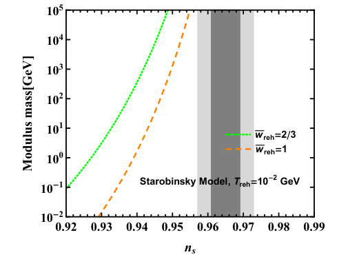
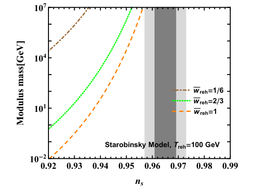
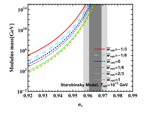
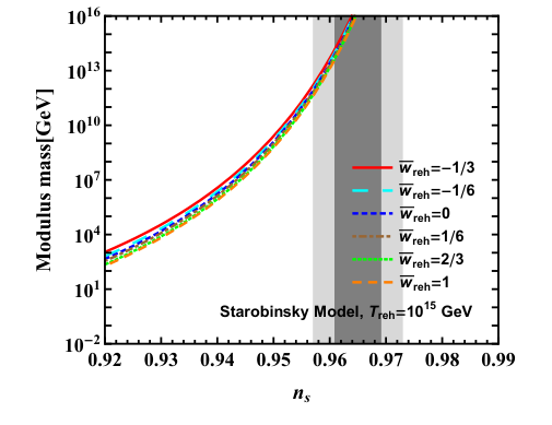
For the Starobinsky model, using Eq. (46), the relation between and for different values of and are shown in figure 4. Similar to the other two models, this starobinsky model also does not predict the value of in the reasonable range for GeV and within Planck’s bounds on . However, with the increase of all corves move towards the central value of , and for GeV all curves predict the value of in the allowed reasonable range within Plancks bounds on .
IV Features in the inflaton potential and constraints on modulus mass
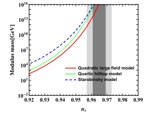
In Ref. Goswami and Yajnik 2018 we showed that the successful explanation of the CMB low multipole anomalies by considering a feature in the inflaton potential the reheating parameters , and can be constrained for the large field, quartic hilltop and Starobinsky models. Using these constraints on the reheating parameters (the upper bounds on ), we plot the modulus mass as a function of the scalar spectral index for different single field inflationary models in Fig. 5. For Planck’s lower limits of , we obtain and GeV respectively for the quadratic large field, quartic hilltop and Starobinsky model. The lower limit of gives GeV, GeV and GeV for the quadratic large field, quartic hilltop and Starobinsky model respectively. The and upper limits of give which rules out late time modulus cosmology.
IV.1 Effects of including in the analysis
As reported by Planck 2018 Akrami et al. 2018, the results for the tensor to scalar ratio are model dependent. The alternative ranges for in conjunction with variation in other parameters are reported in their Table 3. The case that substantially deviates from the others and impacts our results the most corresponds to the inclusion of the effective number of neutrinos, in the analysis. For instance including in the case of Planck TT,TE,EE +lowEB+lensing allows while with error range . The lower limit of this gives GeV, GeV and GeV for the quadratic large field, quartic hilltop and Starobinsky model respectively. Hence this reduces all our answers for by almost orders of magnitude. The central value of this predicts the value of GeV, GeV and GeV for the quadratic large field, quartic hilltop and Starobinsky models respectively.
V Discussion and conclusions
We have obtained a relation among the reheating parameters, the modulus mass and the inflationary observables for single field inflationary models. This is done by tracing the evolution of specific observable scales in CMB from the time of their Hubble crossing during inflation to the present time. This is in principle the same methodology as followed in Dutta and Maharana 2015 which obtained a bound GeV by obtaining a relation between and scalar spectral index . However, by carefully pursuing the analysis and insisting that lies within physically acceptable range and within the phenomenologically constrained range, we obtain a substantially stronger bound. This is shown in Fig.s 2, 3, and 4. Generically our lower bounds on for all models are high, GeV. Conversely, for , the lowest value of reheat temperature we get is GeV obtained by requiring that the modulus mass remains sub-Planckian, . Further, we considered modeling the CMB low multipole anomalies through feature in the inflaton potential. This gives a further handle on the reheat parameters. The simultaneous demand of explaining the CMB anomalies and disappearance of the heavy moduli to accord with observed cosmology requires that GeV depending on the model. An exception to these results arises if, as discussed in Sec. IV.1, one include parameter along with the CDM model in the analysis to determine . This reduces all our bounds on by almost orders of magnitude.
Thus we have leveraged the requirement that the Universe remain Friedmann like, homogeneous and isotropic at all epochs including the reheating phase. This allows us to parameterise the transitory epoch by an effective equation of state parameter for the material content, agnostic of the particle physics details of how this reheating proceeds. The fact that the physically permitted range for this parameter is highly restricted, leads to rather stringent constraints on new physics that may intervene, such as the moduli fields. While a fully detailed model of reheating may provide even more refined information we do have reasonably robust relation of the light moduli mass on other physical parameters. The study may be taken as a demonstration that substantial knowledge about an epoch such as the reheating phase buried deep in the early epochs of the Universe is accessible by CMB observables today.
VI Appendix : Reheating parameters: extension to modulus dominated case
We begin with recapitulating the essentials of the formalism. The inflaton is considering to be governed by a potential undergoing slow-roll evolution with parameters and , resulting in scalar curvature power spectrum and tensor power spectrum as a function of the Fourier transform variable of the argument of the spatial correlation functions, with corresponding indices and . The details of the definitions and notation are standard Liddle and Lyth 1993, and can be found also in the references Riotto 2002; Bassett et al. 2006; Martin et al. 2014. We shall use and , the amplitude of scalar and tensor power spectra at the pivot scale as used by Planck collaboration, . For , these amplitudes are given in terms of as
| (47) |
In terms of the slow-roll parameters and , the tensor to scalar ratio , the scalar spectral index and the tensor spectral index satisfy the relations
| (48) |
The total number of e-foldings, , is defined as the logarithm of the ratio of the scale factor at the final time to it’s value at initial time of the era of inflation.
| (49) |
Where and are the initial and final values of the inflaton field and is the slow-roll parameter defined as . Likewise, given a mode , the number of e-foldings between the time when it crosses the Hubble horizon and the end of inflation is given by
| (50) |
where is the value of the inflaton field at the time of Hubble crossing of the scale k. For the slow-roll approximation i.e., and the Eq. (50) becomes
| (51) |
In the inflationary model of cosmology, at the end of the inflation, the inflaton field decays and reheat the Universe. The energy stored in the inflaton gets converted to radiation. The Hubble parameter and the energy density of the Universe decrease with the expansion of the Universe. When the Hubble parameter’s value becomes equivalent to the mass of a modulus, the modulus field start oscillating in its potential minimum Dutta and Maharana 2015; Das et al. 2015; Coughlan et al. 1983; Banks et al. 1994; de Carlos et al. 1993. The energy density of the modulus field redshifts like matter (which is slower than the redshift rate of radiation); hence, the energy density of the Universe becomes modulus dominated. After this, the modulus decays and reheat the Universe for the second time. During inflation, The equation of motion of a scalar field is given by
| (52) |
Where is the decay width of the scalar field and is the Hubble parameter. If the value of the Hubble parameter is greater than the mass of the scalar, , then the field will freeze at its initial displacement . This initial displacement is of the order of . The quantum fluctuation Goncharov et al. 1984 of the field during inflation or the dependence of the modulus potential on the vacuum expectation value Dine et al. 1984; Coughlan et al. 1984; Dine et al. 1995; Dine et al. 1996; Dutta and Maharana 2015 of the inflaton are the possible reasons for this initial displacement of the scalar field. The modulus starts oscillating around its minimum, and then the energy density of modulus (matter) and radiation becomes equal, and is given by Dutta and Maharana 2015
| (53) |
The energy density of the modulus then dominates, and the modulus decays at energy density
| (54) |
The lifetime of the modulus is expressed as
| (55) |
Using Eqs. (54) and (55) the temperature after the modulus decay can be written in terms of the modulus mass as
| (56) |
The lower bound of the reheat temperature is around a few MeV (the BBN temperature). Hence, using Eq. (56) one obtains the bound on the modulus mass (known as cosmological moduli problem bound) as Coughlan et al. 1983; Banks et al. 1994; de Carlos et al. 1993
| (57) |
References
- Aghanim et al. (2018) N. Aghanim et al. (Planck) (2018), eprint 1807.06209.
- Akrami et al. (2018) Y. Akrami et al. (Planck) (2018), eprint 1807.06211.
- Ade et al. (2016a) P. A. R. Ade et al. (Planck), Astron. Astrophys. 594, A13 (2016a), eprint 1502.01589.
- Ade et al. (2016b) P. A. R. Ade et al. (Planck), Astron. Astrophys. 594, A20 (2016b), eprint 1502.02114.
- Ade et al. (2014a) P. A. R. Ade et al. (Planck), Astron. Astrophys. 571, A22 (2014a), eprint 1303.5082.
- Ade et al. (2014b) P. A. R. Ade et al. (Planck), Astron. Astrophys. 571, A16 (2014b), eprint 1303.5076.
- Dunkley et al. (2009) J. Dunkley et al. (WMAP), Astrophys. J. Suppl. 180, 306 (2009), eprint 0803.0586.
- Komatsu et al. (2009) E. Komatsu et al. (WMAP), Astrophys. J. Suppl. 180, 330 (2009), eprint 0803.0547.
- Komatsu et al. (2011) E. Komatsu, K. M. Smith, J. Dunkley, C. L. Bennett, B. Gold, G. Hinshaw, N. Jarosik, D. Larson, M. R. Nolta, L. Page, et al., The Astrophysical Journal Supplement Series 192, 18 (2011), URL http://stacks.iop.org/0067-0049/192/i=2/a=18.
- Hinshaw et al. (2013) G. Hinshaw, D. Larson, E. Komatsu, D. N. Spergel, C. L. Bennett, J. Dunkley, M. R. Nolta, M. Halpern, R. S. Hill, N. Odegard, et al., The Astrophysical Journal Supplement Series 208, 19 (2013), URL http://stacks.iop.org/0067-0049/208/i=2/a=19.
- Peiris et al. (2003) H. V. Peiris et al. (WMAP), Astrophys. J. Suppl. 148, 213 (2003), eprint astro-ph/0302225.
- Larson et al. (2011) D. Larson, J. Dunkley, G. Hinshaw, E. Komatsu, M. R. Nolta, C. L. Bennett, B. Gold, M. Halpern, R. S. Hill, N. Jarosik, et al., The Astrophysical Journal Supplement Series 192, 16 (2011), URL http://stacks.iop.org/0067-0049/192/i=2/a=16.
- Brown et al. (2009) M. L. Brown, P. Ade, J. Bock, M. Bowden, G. Cahill, P. G. Castro, S. Church, T. Culverhouse, R. B. Friedman, K. Ganga, et al., The Astrophysical Journal 705, 978 (2009), URL http://stacks.iop.org/0004-637X/705/i=1/a=978.
- Reichardt et al. (2009) C. L. Reichardt et al., Astrophys. J. 694, 1200 (2009), eprint 0801.1491.
- Guth and Pi (1982) A. H. Guth and S. Y. Pi, Phys. Rev. Lett. 49, 1110 (1982).
- Starobinsky (1982) A. A. Starobinsky, Phys. Lett. B117, 175 (1982).
- Mukhanov et al. (1992) V. F. Mukhanov, H. A. Feldman, and R. H. Brandenberger, Phys. Rept. 215, 203 (1992).
- Bardeen et al. (1983) J. M. Bardeen, P. J. Steinhardt, and M. S. Turner, Phys. Rev. D28, 679 (1983).
- Riotto (2002) A. Riotto, in Astroparticle physics and cosmology. Proceedings: Summer School, Trieste, Italy, Jun 17-Jul 5 2002 (2002), pp. 317–413, eprint hep-ph/0210162.
- Starobinsky (1980) A. A. Starobinsky, Phys. Lett. 91B, 99 (1980).
- Guth (1981) A. H. Guth, Phys. Rev. D23, 347 (1981).
- Linde (1982) A. D. Linde, Phys. Lett. B108, 389 (1982).
- Hawking (1982) S. W. Hawking, Phys. Lett. 115B, 295 (1982).
- Linde (1983a) A. D. Linde, Phys. Lett. B129, 177 (1983a).
- Linde (2008) A. D. Linde, Lect. Notes Phys. 738, 1 (2008), eprint 0705.0164.
- Martin et al. (2014) J. Martin, C. Ringeval, and V. Vennin, Phys. Dark Univ. 5-6, 75 (2014), eprint 1303.3787.
- Burgess et al. (2013) C. P. Burgess, M. Cicoli, and F. Quevedo, JCAP 1311, 003 (2013), eprint 1306.3512.
- Silverstein (2013) E. Silverstein (2013), eprint 1311.2312.
- Baumann and McAllister (2015) D. Baumann and L. McAllister, Inflation and String Theory, Cambridge Monographs on Mathematical Physics (Cambridge University Press, 2015), ISBN 9781107089693, 9781316237182, eprint 1404.2601, URL http://www.cambridge.org/mw/academic/subjects/physics/theoretical-physics-and-mathematical-physics/inflation-and-string-theory?format=HB.
- Turner (1983) M. S. Turner, Phys. Rev. D28, 1243 (1983).
- Traschen and Brandenberger (1990) J. H. Traschen and R. H. Brandenberger, Phys. Rev. D42, 2491 (1990).
- Albrecht et al. (1982) A. Albrecht, P. J. Steinhardt, M. S. Turner, and F. Wilczek, Phys. Rev. Lett. 48, 1437 (1982).
- Kofman et al. (1994) L. Kofman, A. D. Linde, and A. A. Starobinsky, Phys. Rev. Lett. 73, 3195 (1994), eprint hep-th/9405187.
- Kofman et al. (1997) L. Kofman, A. D. Linde, and A. A. Starobinsky, Phys. Rev. D56, 3258 (1997), eprint hep-ph/9704452.
- Drewes and Kang (2013) M. Drewes and J. U. Kang, Nucl. Phys. B875, 315 (2013), [Erratum: Nucl. Phys.B888,284(2014)], eprint 1305.0267.
- Allahverdi et al. (2010) R. Allahverdi, R. Brandenberger, F.-Y. Cyr-Racine, and A. Mazumdar, Ann. Rev. Nucl. Part. Sci. 60, 27 (2010), eprint 1001.2600.
- Coughlan et al. (1983) G. D. Coughlan, W. Fischler, E. W. Kolb, S. Raby, and G. G. Ross, Phys. Lett. 131B, 59 (1983).
- Banks et al. (1994) T. Banks, D. B. Kaplan, and A. E. Nelson, Phys. Rev. D49, 779 (1994), eprint hep-ph/9308292.
- de Carlos et al. (1993) B. de Carlos, J. A. Casas, F. Quevedo, and E. Roulet, Phys. Lett. B318, 447 (1993), eprint hep-ph/9308325.
- Dutta and Maharana (2015) K. Dutta and A. Maharana, Phys. Rev. D91, 043503 (2015), eprint 1409.7037.
- Goswami and Yajnik (2018) R. Goswami and U. A. Yajnik, JCAP 1810, 018 (2018), eprint 1806.10340.
- Hannestad (2001) S. Hannestad, Phys. Rev. D63, 043009 (2001), eprint astro-ph/0009296.
- Bridle et al. (2003) S. L. Bridle, A. M. Lewis, J. Weller, and G. Efstathiou, Mon. Not. Roy. Astron. Soc. 342, L72 (2003), eprint astro-ph/0302306.
- Mukherjee and Wang (2003) P. Mukherjee and Y. Wang, Astrophys. J. 599, 1 (2003), eprint astro-ph/0303211.
- Hannestad (2004) S. Hannestad, JCAP 0404, 002 (2004), eprint astro-ph/0311491.
- Shafieloo and Souradeep (2004) A. Shafieloo and T. Souradeep, Phys. Rev. D70, 043523 (2004), eprint astro-ph/0312174.
- Shafieloo et al. (2007) A. Shafieloo, T. Souradeep, P. Manimaran, P. K. Panigrahi, and R. Rangarajan, Phys. Rev. D75, 123502 (2007), eprint astro-ph/0611352.
- Shafieloo and Souradeep (2008) A. Shafieloo and T. Souradeep, Phys. Rev. D78, 023511 (2008), eprint 0709.1944.
- Nagata and Yokoyama (2009) R. Nagata and J. Yokoyama, Phys. Rev. D79, 043010 (2009), eprint 0812.4585.
- Nicholson and Contaldi (2009) G. Nicholson and C. R. Contaldi, Journal of Cosmology and Astroparticle Physics 2009, 011 (2009), URL http://stacks.iop.org/1475-7516/2009/i=07/a=011.
- Hazra et al. (2010) D. K. Hazra, M. Aich, R. K. Jain, L. Sriramkumar, and T. Souradeep, JCAP 1010, 008 (2010), eprint 1005.2175.
- Hazra et al. (2016) D. K. Hazra, A. Shafieloo, G. F. Smoot, and A. A. Starobinsky, JCAP 1609, 009 (2016), eprint 1605.02106.
- Hazra et al. (2017) D. K. Hazra, D. Paoletti, M. Ballardini, F. Finelli, A. Shafieloo, G. F. Smoot, and A. A. Starobinsky (2017), eprint 1710.01205.
- Starobinsky (1992) A. A. Starobinsky, JETP Lett. 55, 489 (1992), [Pisma Zh. Eksp. Teor. Fiz.55,477(1992)].
- Dvorkin and Hu (2010) C. Dvorkin and W. Hu, Phys. Rev. D81, 023518 (2010), eprint 0910.2237.
- Adams et al. (2001) J. A. Adams, B. Cresswell, and R. Easther, Phys. Rev. D64, 123514 (2001), eprint astro-ph/0102236.
- Covi et al. (2006) L. Covi, J. Hamann, A. Melchiorri, A. Slosar, and I. Sorbera, Phys. Rev. D74, 083509 (2006), eprint astro-ph/0606452.
- Hamann et al. (2007) J. Hamann, L. Covi, A. Melchiorri, and A. Slosar, Phys. Rev. D76, 023503 (2007), eprint astro-ph/0701380.
- Mortonson et al. (2009) M. J. Mortonson, C. Dvorkin, H. V. Peiris, and W. Hu, Phys. Rev. D79, 103519 (2009), eprint 0903.4920.
- Joy et al. (2008) M. Joy, V. Sahni, and A. A. Starobinsky, Phys. Rev. D77, 023514 (2008), eprint 0711.1585.
- Jain et al. (2009) R. K. Jain, P. Chingangbam, J.-O. Gong, L. Sriramkumar, and T. Souradeep, JCAP 0901, 009 (2009), eprint 0809.3915.
- Jain et al. (2010) R. K. Jain, P. Chingangbam, L. Sriramkumar, and T. Souradeep, Phys. Rev. D82, 023509 (2010), eprint 0904.2518.
- Garg and Yajnik (2018) I. Garg and U. A. Yajnik, Phys. Rev. D98, 063523 (2018), eprint 1802.03915.
- Kane et al. (2015) G. Kane, K. Sinha, and S. Watson, Int. J. Mod. Phys. D24, 1530022 (2015), eprint 1502.07746.
- Das et al. (2015) K. Das, K. Dutta, and A. Maharana, Phys. Lett. B751, 195 (2015), eprint 1506.05745.
- Cicoli et al. (2016) M. Cicoli, K. Dutta, A. Maharana, and F. Quevedo, JCAP 1608, 006 (2016), eprint 1604.08512.
- Bhattacharya et al. (2017) S. Bhattacharya, K. Dutta, and A. Maharana, Phys. Rev. D96, 083522 (2017), [Addendum: Phys. Rev.D96,no.10,109901(2017)], eprint 1707.07924.
- Bhattacharya et al. (2018) S. Bhattacharya, K. Dutta, M. R. Gangopadhyay, and A. Maharana, Phys. Rev. D97, 123533 (2018), eprint 1711.04807.
- Maharana and Zavala (2018) A. Maharana and I. Zavala, Phys. Rev. D97, 123518 (2018), eprint 1712.07071.
- Boyanovsky et al. (1996) D. Boyanovsky, H. J. de Vega, R. Holman, and J. F. J. Salgado, in String theory in curved space times. Proceedings, String Gravity Meeting, Paris, France, June 6-7, 1996 (1996), pp. 260–280, eprint astro-ph/9609007.
- Kofman (1997) L. Kofman, in Particle cosmology. Proceedings, 3rd RESCEU International Symposium, Tokyo, Japan, November 10-13, 1997 (1997), pp. 1–8, eprint hep-ph/9802285.
- Felder et al. (1999) G. N. Felder, L. Kofman, and A. D. Linde, Phys. Rev. D59, 123523 (1999), eprint hep-ph/9812289.
- Giudice et al. (2001) G. F. Giudice, A. Riotto, and I. I. Tkachev, JHEP 06, 020 (2001), eprint hep-ph/0103248.
- Desroche et al. (2005) M. Desroche, G. N. Felder, J. M. Kratochvil, and A. D. Linde, Phys. Rev. D71, 103516 (2005), eprint hep-th/0501080.
- Martin (2004) J. Martin, Braz. J. Phys. 34, 1307 (2004), eprint astro-ph/0312492.
- Martin et al. (2015) J. Martin, C. Ringeval, and V. Vennin, Phys. Rev. Lett. 114, 081303 (2015), eprint 1410.7958.
- Allahverdi et al. (2018) R. Allahverdi, K. Dutta, and A. Maharana, JCAP 10, 038 (2018), eprint 1808.02659.
- Dai et al. (2014) L. Dai, M. Kamionkowski, and J. Wang, Phys. Rev. Lett. 113, 041302 (2014), eprint 1404.6704.
- Linde (1983b) A. D. Linde, JETP Lett. 38, 176 (1983b), [Pisma Zh. Eksp. Teor. Fiz.38,149(1983)].
- Bassett et al. (2006) B. A. Bassett, S. Tsujikawa, and D. Wands, Rev. Mod. Phys. 78, 537 (2006), eprint astro-ph/0507632.
- Kinney and Mahanthappa (1996) W. H. Kinney and K. T. Mahanthappa, Phys. Lett. B383, 24 (1996), eprint hep-ph/9511460.
- Kehagias et al. (2014) A. Kehagias, A. Moradinezhad Dizgah, and A. Riotto, Phys. Rev. D89, 043527 (2014), eprint 1312.1155.
- Cook et al. (2015) J. L. Cook, E. Dimastrogiovanni, D. A. Easson, and L. M. Krauss, JCAP 1504, 047 (2015), eprint 1502.04673.
- Liddle and Lyth (1993) A. R. Liddle and D. H. Lyth, Phys. Rept. 231, 1 (1993), eprint astro-ph/9303019.
- Goncharov et al. (1984) A. S. Goncharov, A. D. Linde, and M. I. Vysotsky, Phys. Lett. 147B, 279 (1984).
- Dine et al. (1984) M. Dine, W. Fischler, and D. Nemeschansky, Phys. Lett. 136B, 169 (1984).
- Coughlan et al. (1984) G. D. Coughlan, R. Holman, P. Ramond, and G. G. Ross, Phys. Lett. 140B, 44 (1984).
- Dine et al. (1995) M. Dine, L. Randall, and S. D. Thomas, Phys. Rev. Lett. 75, 398 (1995), eprint hep-ph/9503303.
- Dine et al. (1996) M. Dine, L. Randall, and S. D. Thomas, Nucl. Phys. B458, 291 (1996), eprint hep-ph/9507453.