09.08.2019
Keywords: Unstable dynamics, divergent trajectories, conditional process, quasi-stationary distribution, Q-process, Doob’s h-transform
Living on the edge of instability
Abstract
Statistical description of stochastic dynamics in highly unstable potentials is strongly affected by properties of divergent trajectories, that quickly leave meta-stable regions of the potential landscape and never return. Using ideas from theory of Q-processes and quasi-stationary distributions, we analyze position statistics of non-diverging trajectories. We discuss two limit distributions which can be considered as (formal) generalizations of the Gibbs canonical distribution to highly unstable systems. Even though the associated effective potentials differ only slightly, properties of the two distributions are fundamentally different for all highly unstable system. The distribution for trajectories conditioned to diverge in an infinitely distant future is localized and light-tailed. The other distribution, describing trajectories surviving in the meta-stable region at the instant of conditioning, is heavy-tailed. The exponent of the corresponding power-law tail is determined by the leading divergent term of the unstable potential. We discuss different equivalent forms of the two distributions and derive properties of the effective statistical force arising in the ensemble of non-diverging trajectories after the Doob h-transform. The obtained explicit results generically apply to non-linear dynamical models with meta-stable states and fast kinetic transitions.
1 Introduction
Unstable stochastic dynamics is ubiquitous in non-linear models. Its characteristic feature is fast divergence of trajectories that have left a meta-stable state. The divergence restricts precision and duration of experiments [1, 2], and limits applicability of the standard statistical analysis based on the averages, because the latter rapidly diverge with time [3, 4, 5].
In recent theoretical and experimental works [5, 2], the standard description based on moments has been replaced by analysis of local characteristics of the system given by the mode and the curvature near the maximum of the probability density function. The second important point was the shift of attention from the complete ensemble of trajectories to the conditional statistics of non-divergent ones. This allowed to obtained a detailed picture of the unstable dynamics. The theory has been applied to the paradigmatic case of the one-dimensional overdamped Brownian motion
| (1) |
in the highly unstable cubic potential
| (2) |
Above, the standard Gaussian white noise satisfies , , and the diffusion coefficient is proportional to the thermal energy in accordance with the Einstein relation , where stands for the friction constant.
The main focus of the aforementioned works has been on the short-time dynamics, zero-noise limit and the so-called quasi-stationary distribution in highly unstable systems. In the present work, we use ideas from the probabilistic theory of conditioned stochastic processes [6, 7] and derive generic behavior of non-diverging trajectories.
First, in Sec. 2, we define precisely what we understand by highly unstable dynamics, demonstrate typical features of trajectories, and emphasize that their divergence is related to the loss of normalization of the propagator. In Sec. 3, we show that highly unstable systems have a discrete spectrum and prove an identity for the generalized partition function. The latter allows us to derive tails of the both discussed limit distributions (Sec. 5.1 and Sec. 6), and the magnitude of an effective statistical force arising in the conditioned ensemble from the Doob h-transform [8] (5.2).
The quasi-stationary distribution (Sec. 6) and the limit distribution of the trajectories that never diverge (Sec. 5) can be regarded as generalizations of the Gibbs canonical distribution to appropriate ensembles of highly unstable systems. Both these distributions reduce to the Gibbs canonical one for stable potentials. Analysis of their properties generic for highly unstable dynamics, particularly based on the notion of effective potentials, are the main topic of the present work.
Alternative methods that can be successfully applied to study highly unstable dynamics include analysis of first-passage times [9, 10, 11, 12, 13, 14, 15, 16, 17, 18, 19, 20, 21, 22, 23, 24, 1], and of the so-called nonlinear relaxation times [25, 26]. The analysis of times yields e.g. transition rates for unstable processes. Our present approach is complementary to these methods in the sense that it provides a detailed picture of the particle position statistics in different naturally arising conditional ensembles.
2 Highly unstable dynamics
By highly unstable dynamics we shall understand an overdamped Brownian motion in a potential decreasing towards for large so fast that the particle reaches (minus) infinity in a finite time. We shall call such potentials as highly unstable. Equivalently, they can be defined as the class of potentials for which the mean first-passage time from any point to is finite [24].
The simplest examples of highly unstable potentials include the cubic, and the inverted quartic potentials. Generally speaking, highly unstable potentials decrease towards minus infinity at least as for large , with . To see that such potentials are highly unstable, we inspect the zero-noise limit of the Langevin equation (1) with when . For the initial condition placed into the unstable region, , we obtain the deterministic solution
| (3) |
This solution reaches minus infinity at the finite time , when the denominator attains zero. Notice that for the inverted parabolic potential (), we get the exponential divergence of . Even though the exponential divergence can be considered as “fast” in some contexts, it is much “slower” than the divergence generated by Eq. (3). Therefore, the inverted parabolic potential is not highly unstable.
Equivalently, one can determine the condition starting from the exact expression for the mean-first passage time to (minus) infinity. The mean time is known analytically in one dimension [27]. For the detailed discussion related to the high instability of the cubic potential see e.g. Ref. [24] and references therein.
Figure 1(b) shows a typical sample of trajectories starting at and diffusing in the highly unstable cubic potential. A trajectory in the sample can consist of three distinct segments. First, on the potential plateau, i.e., in the region near the origin approximately determined by the condition that the cubic potential is weak compared to thermal energy, , the trajectory undergoes the (almost) free diffusion. Second, occasionally, the trajectory is reflected by the strong cubic repulsion and returns quickly to the plateau if it reaches a large positive [upward spikes in Fig. 1(b)]. Third, the last part of the trajectory begins if the particle moves left from the plateau and reaches highly unstable region . There, the decreasing branch of the cubic potential is extremely strong compared to the thermal noise, , and the trajectory is quickly dragged towards minus infinity. The divergence is nearly deterministic, in accord with Eq. (3) for .

A characteristic feature of highly unstable dynamics, which we prove in Sec. 3, is that the Fokker-Planck operator corresponding to the Langevin equation (1),
| (4) |
has a discrete spectrum of eigenvalues
| (5) |
| (6) |
That is, for highly unstable dynamics, there exists an isolated leading decay rate , and the strictly positive gap
| (7) |
between the eigenvalues corresponding to the slowest and the second-slowest decaying modes.
The propagator, or the probability density function (PDF) of the particle position at time , given that initially the particle was at , satisfies the Fokker-Planck equation
| (8) |
The eigenvalues determine decay rates of individual modes with amplitudes given by the eigenfunctions defined in Eq. (6). The propagator can be expressed in terms of the eigenfunctions as [28]
| (9) |
Above, the functions depend on the initial particle position, , and follow from the adjoint eigenvalue problem
| (10) |
with the operator
| (11) |
adjoint to the Fokker-Planck operator . The adjoint operator is called the generator of the Markov process. The two sets of eigenfunctions satisfy the following normalization conditions
| (12) | |||||
| (13) |
We shall refer to and as the right and left eigenfunctions of the Fokker-Planck operator , respectively.
The high instability of dynamics manifests itself through exponential decay of normalization of the propagator (9). The normalization equals to the probability that a trajectory has not diverged up to time and thus we call it as the survival probability [9]. In symbols, we have
| (14) |
Above, stands for the time of divergence of a trajectory. According to Eq. (9), in the long-time limit only the most-slowly decaying term contributes significantly to the sum, i.e.,
| (15) |
which we will simply write as
| (16) |
and
| (17) |
where “” means that the ratio of the two expressions converges to unity with increasing time.
Physical meaning of the exponential decay (17) can be understood based on the illustration in Fig. 1(b). The decay arises from the fast divergence of majority of the trajectories which reach in a finite time. They are not included in the statistics described by the propagator for any finite , , and their weight is given by .
Finally, notice that for a confining potential , the dynamics becomes stable and conservative, and we have , , and , where the equilibrium partition function ensures the normalization condition, . Contrary to this, in the highly unstable non-conservative case, the eigenfunction is no-longer constant. Below, we shall see that the expressions and , which are identical in the stable case, play roles of stationary distributions in proper conditioned ensembles of non-diverging trajectories. The two ensembles, described by these distributions, have fundamentally different statistical properties, cf. Sec. 5.1 and Sec. 6.
3 Schrödinger equation: Normalization of eigenvectors
The eigenproblem for the non-Hermitian Fokker-Planck operator involves distinct left and right eigenfunctions for each eigenvalue . The two sets of eigenfunctions satisfy different boundary conditions and should be normalized properly to form orthogonal spaces, as we have described above in Sec. 2.
The non-Hermitian eigenproblem can be transformed into the regular Hermitian one by a similarity transformation that recasts the Fokker-Planck operator (or equivalently the generator) into the Hermitian Hamiltonian [29, 27, 30]:
| (18a) | |||||
| (18b) | |||||
| (18c) | |||||
where , and the diffusion coefficient, , determines the inverse mass of the representative quantum particle. The transformed potential,
| (18s) |
is confining for all highly unstable potentials . For the cubic potential, is a quartic well [the term proportional to ] with a slight asymmetry and shift of the minimum caused by the linear term arising from , see Fig. 2.
The transformation provides two valuable insights. The first results from the discrete structure of the spectrum of that is equivalent to the discrete well-separated spectrum of . Indeed, the spectrum of is identical to that of up to the sign:
| (18t) |
Because is always confining for highly unstable , the spectrum is always discrete as it is the case for all confining infinite potential wells [31]. Therefore, the inequalities (5) follow directly from the high instability of .
The second insight arises from the transformation between the wave functions and eigenfunctions of . The ground state wave function, associated with the energy , is related to the eigenfunctions and of via
| (18u) | |||
| (18v) |
respectively. The factor is independent of and it plays no role in the construction of the propagator (9) for the diffusion problem. Hence, is usually omitted in standard literature, e.g. [29, 27, 30], when discussing the spectral solution of the Fokker-Planck equation. On the contrary, the factor , to which we shall refer as to the generalized partition function, is fundamental for the understanding of the Q-process.
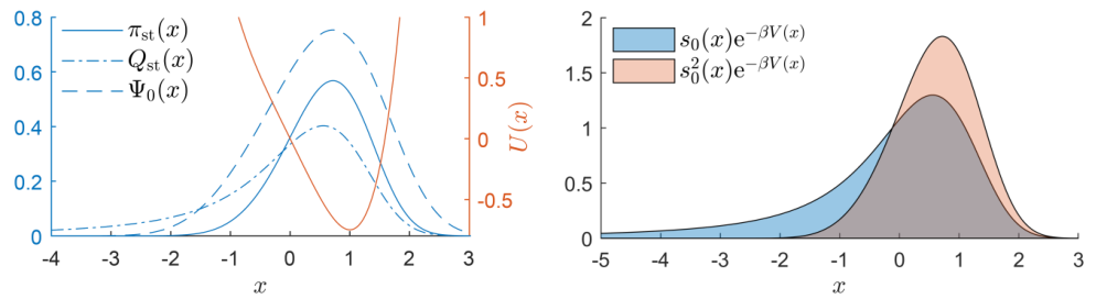
Two equivalent integral representations of the partition function, used below to explore properties of stationary distributions, are
| (18wa) | |||||
| (18wb) | |||||
Hence, we obtain the identity
| (18wx) |
Even though the functions and are strikingly different, they enclose equal areas. Figure 2 shows both the localized function with light tails, and the function possessing a heavy tail for negative .
The identity (18wx) follows from the normalization conditions (12) and (13), which, for the eigenfunctions and , read
| (18wy) | |||||
| (18wz) |
The combination of Eqs. (18u) and (18v) yields
| (18waa) | |||
| (18wab) |
The requirement that right-hand sides of both equations are normalized to unity immediately gives us the identity (18wx). In other words, the constant in Eqs. (18u) and (18v) is crucial for consistency of Eqs. (18waa) and (18wab), relating the eigenfunctions and , with the normalization conditions (18wy) and (18wz).
For the Gibbs canonical equilibrium distribution in a confining potential , the generalized partition function is identical to the equilibrium partition function. In equilibrium, we have , , and the corresponding right eigenfunction of is the Gibbs canonical distribution , with .
4 Q-process: Dynamics
Figure 1(c) shows three distinct dynamical regimes observed on trajectories that do not diverge in a highly unstable potential . In the transient regime I, the relaxation of the initial condition takes place. In the stationary regime II, the initial condition is already forgotten and the ensemble of trajectories resembles sample paths of a stationary conservative process diffusing away from the instability region. Within II, the particle position is described by the time-independent PDF . Finally, in the transient regime III, the distribution departs from and approaches the heavy-tailed quasi-stationary distribution discussed in Sec. 6.
Durations of the transient regimes I and III can be estimated by the inverse difference of decay rates , , that is finite due to high instability of . The finite transient times allow for an exact statistical description of trajectories in the regimes I and II. Formally, this is done by shifting the last transient regime III towards infinite times. This limit has no significant influence on trajectory statistics within regimes I and II. Remarkably, the limit transforms the non-Markovian process, conditioned on a non-local property (non-divergence up to a given time), into a Markovian one, that can be analyzed using standard tools as the Langevin and the Fokker-Planck equation.
Let us choose an “intermediate” time , and the “final” time of conditioning , such that . In Fig. 1(c), we have and . All trajectories of interest are assumed to diverge after time . That is, the time of divergence of any trajectory satisfies . Now, we can formally shift the conditioning time to infinity and define the distribution of trajectories at finite time :
| (18wac) |
The limit means that the process is conditioned to never diverge. In mathematical literature, such a process is commonly denoted as the Q-process [32, 33].
The propagator for the Q-process is derived by a direct evaluation of the above limit. Employing the Markov property, we rewrite the joint probability density in (18wac) as the product of propagators for the intervals and : . Then, for large and fixed , we get
| (18wad) |
The conditioning time cancels out and the integral over equals to one. The limit shifts the time of conditioning and the whole transient region III in Fig. 1(c) towards infinite times and removes information on III from the dynamics of trajectories at any fixed .
The right-hand side of Eq. (18wad) yields explicit form of the propagator for the Q-process:
| (18wae) |
It is straightforward to verify that the Q-process is a conservative Markov process. The normalization condition, , is verified most easily using the eigenfunction expansion of (9) and the orthogonality relation for the eigenfunctions (13). The Chapman-Kolmogorov equation, , follows directly from the Chapmann-Kolmogorov equation for the bare propagator .
The Q-process is the driven diffusion process and, as such, its propagator satisfies the backward equation
| (18waf) |
with the generator
| (18waga) | |||||
| (18wagb) | |||||
The generator (18waga) is obtained directly by taking the time derivative of Eq. (18wae), and using that . The explicit form (18wagb) follows from (18waga) after some algebra. The Fokker-Planck operator adjoint to the generator reads
| (18wagaha) | |||||
| (18wagahb) | |||||
Equivalently, the dynamics of trajectories can be described by the Langevin equation corresponding to the Fokker-Planck operator (18wagahb),
| (18wagahai) |
In mathematics, the similarity transformation (18waga) is known as the Doob h-transform [8]. It leaves intact the diffusion coefficient and introduces an effective drift that keeps the trajectories away from the unstable region of the potential. For a more rigorous discussion of the Q-process, we refer to the extensive mathematical literature on the topic, see e.g. [7] and references therein. Here, our aim was to introduce these concepts heuristically and accessibly for a wide audience of physicists.
In physics, an analogue of the Q-process can be found in theory of large deviations as one of effective processes that can be used to generate ensembles associated with rare values of time-extensive observables [34, 35, 36, 37, 38, 39]. For a comprehensive review of Markov processes conditioned on large deviations see Ref. [6], where also the connection to the original Doob’s conditioning is described in a great detail.
5 Q-process: Limit distribution
For any initial condition, the dynamics of Q-process converges towards the stationary regime II with the relaxation time . The limit distribution of the Q-process can be computed as the long-time limit of its propagator,
| (18wagahaj) |
The first equality shows that any trace of the initial condition is forgotten. The second one emphasizes importance of correct ordering of the two limits and suggests that the limit distribution differs from the quasi-stationary distribution . The latter appears at the final instant of the transient regime III, which we have shifted to infinity before taking the limit , cf. Eq. (18wac) and Eq. (18wagahbe) below.
The limit distribution describes the stationary state of trajectories which will diverge in (an infinitely) distant future. The explicit evaluation of the limit with the aid of the leading asymptotic behavior of the propagator (16) yields
| (18wagahak) |
Hence the limit distribution is given by
| (18wagahal) |
The PDF is the stationary distribution (corresponding to the eigenvalue 0) of the Fokker-Planck operator (18wagahb). The equality can be verified directly by applying the Fokker-Planck operator (18wagaha) on the PDF (18wagahal).
The relations (18u) and (18v), between the eigenfunctions , and the ground state wave function reveal the physical meaning of :
| (18wagaham) |
The equality implies that powerful quantum-mechanical methods for approximating ground state wave functions can be applied to discuss for highly unstable dynamics.
Another expression for follows from the relation (18wab) between the eigenfunctions and established in Sec. 3,
| (18wagahan) |
In this form, resembles the Gibbs canonical distribution with the density of states , and . The divergence of the Boltzmann factor for is compensated by the fast decrease of the squared eigenfunction , accounting for the fact that the non-diverging trajectories do not populate the unstable region , and thus the PDF is normalizable.
Last but not least, it is convenient to reshape Eq. (18wagahan) into the Gibbs canonical form containing an effective potential . The result is
| (18wagahao) |
where
| (18wagahap) |
The minus derivative of gives us the effective force,
| (18wagahaq) |
arising from the tendency of non-diverging trajectories to avoid the highly unstable region . In the Langevin equation (18wagahai) and in the corresponding Fokker-Planck operator (18wagahb), the force (18wagahaq) acts in a superposition with the actual external drift force given by .
Even though the limit distribution of the non-diverging trajectories (18wagahao) and the generalized partition function (18wb) are formally similar to their counterparts in the equilibrium canonical ensemble, there is an important physical difference. In the equilibrium case, both and are determined solely by the temperature and the external potential . On the contrary, and for the Q-process depend also on the friction constant through the eigenfunction .
Hence, and for non-diverging trajectories are kinetic quantities whose values depend on time scales involved in the problem [and not only on the temperature and the external potential ]. Qualitatively similar situation appears in theory of non-equilibrium steady states of processes driven by e.g. couplings to several reservoirs with different chemical potentials and temperatures, or/and by non-conservative external forces. In such steady states, kinetic parameters like friction coefficients (called also non-dissipative or frenetic) often determine the overall shape of the stationary probability distribution and magnitudes of the corresponding currents [40, 41, 42, 43, 44].
Analogous strong dependencies on kinetic parameters can be expected for the limit distribution of non-diverging trajectories in highly unstable dynamics. The two cases exhibit an interesting difference in the mathematical structure of the probability distributions. In the non-equilibrium steady states, we have and both the kinetic and the thermodynamic effects are mixed in a single PDF given by . On the other hand, in the highly unstable dynamics, the two effects are separated and contained within the two contributions to the effective potential (18wagahap). Further investigation in this direction, focusing in particular on higher-dimensional models, may reveal new interesting phenomena for conditioned processes.
5.1 Tails of the limit distribution and effective potential
For large outside the unstable region, the eigenfunction [and the potential ] approaches a constant and the force , repelling non-diverging trajectories from the highly unstable region, vanishes. Hence the right tail of the limit distribution can be approximated by the Boltzmann tail:
| (18wagahar) |
In this sense, the force is short-ranged and has no significant effect on dynamics for , where the effective potential in Eq. (18wagahao) is given by the actual external potential, , for .
The left tail of the limit distribution can be inferred directly from the definition of in Eq. (18wa) and the eigenvalue equation for ,
| (18wagahas) |
We multiply the equation with the Boltzmann factor and integrate over . Equation (18wa) assures that the integral is convergent and appears on the left-hand side. After the integration, we obtain
| (18wagahat) |
Therefore, the controlling asymptotic factor of for is the exponential . It is straightforward to verify that the above limit is satisfied by the function
| (18wagahau) |
The limit distribution thus decays exponentially as
| (18wagahav) |
the exponential decay being modified by a polynomial prefactor determined by the unstable part of , . Note that the constant prefactor in this equation is exact because it follows from the limit on the right-hand side of Eq. (18wagahat).
The result (18wagahav) provides complete information on the asymptotic behavior of the total effective potential in Eq. (18wagahao) and in particular on its part arising due to the conditioning. The latter behaves as
| (18wagahaw) |
The first term on the right-hand side compensates the external unstable potential and contributes by the exponent responsible for the exponential decay in Eq. (18wagahau). The second term creates a logarithmic barrier . Interestingly enough, the barrier is impenetrable for all cases of interest in the present paper where ; for a further discussion see classification of boundary conditions for the Bessel process, e.g. in Refs. [45, 46]. Finally, we emphasize that the relation (18wagahaw) holds only asymptotically, i.e., the effective potential has no singularity around where majority of non-diverging trajectories live.
5.2 Mean squared force
Having understood the asymptotic behaviors of the effective potential , it is interesting to ask, what is an average magnitude of the force and how it depends on the model parameters , , , and . A simple answer is provided in this Section. It is based on the second expression for in Eq. (18wb) and on a scaling analysis.
Intuitively we expect the magnitude of the force to increase with the degree of instability. Indeed, it turns out that the mean squared amplitude of the force is proportional to the decay rate
| (18wagahax) |
The average is taken with respect to . Equation (18wagahax) follows directly from the differential equation (18wagahas) for , and from Eq. (18wa) for the partition function containing the second power of . We multiply both sides of Eq. (18wagahas) by , integrate over , identify on the right-hand side in accordance with Eq. (18wb), and get
| (18wagahay) |
where we have performed the per partes integration on the right-hand side. After dividing Eq. (18wagahay) with and adjusting properly the factor, we get Eq. (18wagahax).
Equation (18wagahax) is valid generally for any potential . Its further explicit analysis is possible for monomial unstable potentials via the scaling analysis. Defining the time and the length scales as [2]
| (18wagahaz) |
respectively, the eigenvalue problem (6) attains the dimensionless form
| (18wagahba) |
where stands for the transformed coordinate variable, and the transformed dimensionless decay rate , depends on the order only. Similar transformation can be applied to the adjoint eigenvalue problem for the left eigenfunctions.
Rescaling the position variable by and the decay rate with , we obtain from the exact equation (18wagahax) the explicit dependence
| (18wagahbb) |
of the force magnitude on the model parameters. Similar dependence holds for the mean value of the force,
| (18wagahbc) |
where the prefactor depends on only.
The effective force always increases with the temperature and with the potential amplitude . The dependence on becomes weaker for larger powers , which suppress the potential magnitude at the plateau around , where majority of non-diverging trajectories live. For large , the temperature dependence in (18wagahbc) becomes linear for the same reason.
6 Quasi-stationary distribution
In this section, we compare the limit distribution of the Q-process and the quasi-stationary distribution . The latter arises at the end of the transient regime III in Fig. 1(c). Specifically, we shall use the derived properties of the effective potential and relations between the eigenvectors to illustrate the most striking difference between the two distributions.
The statistics of trajectories at time that are non-diverging at least up to time is characterized by the conditional PDF
| (18wagahbd) |
where the inequality means that each trajectory in the conditioned ensemble diverges later than at . In contrast to Eq. (18wac), here, the time of conditioning is identical with the time of observation of the process. Existence of the spectral gap implies that the conditioned PDF (18wagahbd) converges exponentially fast to the limit
| (18wagahbe) |
The limit is known as the quasi-stationary distribution in mathematical literature, where it has first been introduced in context of branching processes and absorbed Marov chains [47, 48, 49, 50] and since then has been studied extensively in context of population dynamics with extinction [7]. The extinction event in population dynamics is in our context represented by the trajectory divergence.
Evaluation of the limit (18wagahbe) with the aid of the long-time expressions (16) and (17) for and , respectively, shows that it is equal to the eigenfunction , i.e.,
| (18wagahbf) |
Then, Eq. (18waa) can be used to recast this relation into the form
| (18wagahbg) |
analogous to the one we have examined for , cf. Eq. (18wagahan). The two equations differ just by a power of on their right-hand sides. The generalized partition functions are equal in the both equations because of the identity (18wx), expressing that areas enclosed by nominators in Eqs. (eq:Qsts0) and (18wagahan) are the same even though the two functions are rather different, as illustrated in the right panel of Fig. 2.
To pursue the comparison further, the quasi-stationary distribution (18wagahbg) can be written in the form
| (18wagahbh) |
resembling the canonical-like expression for in Eq. (18wagahao). There is just a minor difference between expressions for the two distributions given by the factor in the above exponent, i.e., . This minor difference has no effect on the right tail of the quasi-stationary distribution. Hence the tail is the same as that of in Eq. (18wagahar),
| (18wagahbi) |
because of converges of to a constant.
Contrary to the similarity of right tails, the factor in Eq. (18wagahbh) strongly influences the asymptotic behavior for . Based on Eq. (18wagahau), the left tail assumes the form
| (18wagahbj) |
Specifically, for the tail decays as the power law
| (18wagahbk) |
Hence, in contrast to in the Q-process limit distribution (18wagahao), the modified effective potential in the present case of the quasi-stationary distribution (18wagahbh), , is not strong enough to confine trajectories to the stable region. The power-law decay (18wagahbk), arising from the asymptotically logarithmic potential in Eq. (18wagahbh),
| (18wagahbl) |
allows trajectories to populate any negative exploring the whole unstable region with a slowly decaying probability.
Note that for the cubic potential, no integer moments of the quasi-stationary distribution exist and hence the standard statistical analysis of particle position based on averages provides no information on the actual particle dynamics. An alternative approach based on local quantities (position of the PDF maximum and curvature near the maximum) has been proposed [3, 5] and its utility verified experimentally in [2] on colloidal particles diffusing in a nonlinear optical trap illustrated in Fig. 1(a).
We also note that it is possible to construct an effective conservative Markov process that converges towards the distribution in the long-time limit [5]. The process is based on an appropriate return (or resetting) of the diverging trajectories. The effective process should not be confused with the Q-process discussed above. The two has different limiting distributions and the Q-process describes faithfully the conditioned dynamics whereas the effective process of Ref. [5] converges towards only asymptotically in the long-time limit and its transient dynamics may differ from the actual one.
7 Conclusions and perspectives
We have discussed properties of the position statistics of non-diverging stochastic trajectories diffusing in highly unstable potentials. Two stationary distributions arising in this case can be formally expressed in the Gibbs canonical form with the effective potentials depending on the left eigenvector of the Fokker-Planck operator.
The limit distribution of the Q-process describes stationary statistics of trajectories conditioned to be non-diverging for an infinitely long time. For all highly unstable systems, the distribution is localized with exponentially decaying tails. The effective force arising from the conditioning keeps trajectories away from the unstable region of the potential and its strength increases with the degree of instability.
On the other hand, the quasi-stationary distribution is heavy-tailed towards the instability and hence it allows trajectories to be located anywhere in the unstable region. The slow power-law decay of the quasi-stationary distribution is determined by the derivative of the external potential, cf. Eq. (18wagahbk). Here, an interesting question arises whether the theory of non-normalizable distributions [51] may contribute to our understanding of unstable dynamics with non-integer exponents smaller than 3.
As shown in Sec. 3, the basic property of highly unstable potentials is that the spectrum of the Fokker-Planck operator is negative and discrete. Other systems satisfying the same property include confined diffusions with absorbing boundaries. At the same time, our results imply that the magnitude of the effective force, which confines conditioned trajectories of the Q-process, decreases with the decreasing instability of the potential, cf. Sec. 5.2. Therefore, it may be interesting to explore the dynamics for other unstable potentials and identify the precise conditions, when the Q-process becomes transient.
Finally, we remark that the similarity of the two distributions with the Gibbs canonical ensemble is purely formal. In general, the distributions for the highly unstable systems, depended on kinetic parameters such as the friction coefficients. This dependence implies a remarkable possibility to control the overall shape of the two distributions by varying the kinetic parameters only. This effect should become more pronounced in higher-dimensional systems and it represents another interesting area for a further investigation.
References
References
- [1] Šiler M, Jákl P, Brzobohatý O, Ryabov A, Filip R and Zemánek P 2017 Sci. Rep. 7 1697 URL https://doi.org/10.1038/s41598-017-01848-4
- [2] Šiler M, Ornigotti L, Brzobohatý O, Jákl P, Ryabov A, Holubec V, Zemánek P and Filip R 2018 Phys. Rev. Lett. 121 230601 URL https://doi.org/10.1103/PhysRevLett.121.230601
- [3] Filip R and Zemánek P 2016 J. Opt. 18 065401 URL https://doi.org/10.1088/2040-8978/18/6/065401
- [4] Zemánek P, Šiler M, Brzobohatý O, Jákl P and Filip R 2016 J. Opt. 18 065402 URL https://doi.org/10.1088/2040-8978/18/6/065402
- [5] Ornigotti L, Ryabov A, Holubec V and Filip R 2018 Phys. Rev. E 97 032127 URL http://doi.org/10.1103/PhysRevE.97.032127
- [6] Chetrite R and Touchette H 2015 Ann. Henri Poincaré 16 2005 URL https://doi.org/10.1007/s00023-014-0375-8
- [7] Collet P, Martínez S and San Martín J 2013 Quasi-Stationary Distributions: Markov Chains, Diffusions and Dynamical Systems (Springer-Verlag Berlin Heidelberg) ISBN 978-3-642-33130-5 URL https://doi.org/10.1007/978-3-642-33131-2
- [8] Doob J L 2001 Classical Potential Theory and Its Probabilistic Counterpart (Springer-Verlag Berlin Heidelberg) ISBN 978-3-540-41206-9 URL https://doi.org/10.1007/978-3-642-56573-1
- [9] Redner S 2001 A Guide to First-Passage Processes (Cambridge University Press) ISBN 9780511606014 URL https://doi.org/10.1017/CBO9780511606014
- [10] Hänggi P, Talkner P and Borkovec M 1990 Rev. Mod. Phys. 62 251–341 URL https://doi.org/10.1103/RevModPhys.62.251
- [11] Arecchi F T, Politi A and Ulivi L 1982 Il Nuovo Cimento B (1971-1996) 71 119–154 URL http://dx.doi.org/10.1007/BF02721698
- [12] Young M R and Singh S 1985 Phys. Rev. A 31(2) 888–891 URL https://doi.org/10.1103/PhysRevA.31.888
- [13] Colet P, San Miguel M, Casademunt J and Sancho J M 1989 Phys. Rev. A 39 149–156 URL https://doi.org/10.1103/PhysRevA.39.149
- [14] Hirsch J E, Huberman B A and Scalapino D J 1982 Phys. Rev. A 25 519–532 URL https://doi.org/10.1103/PhysRevA.25.519
- [15] Sigeti D and Horsthemke W 1989 J. Stat. Phys. 54 1217–1222 URL http://dx.doi.org/10.1007/BF01044713
- [16] Ramírez-Piscina L and Sancho J M 1991 Phys. Rev. A 43 663–668 URL https://doi.org/10.1103/PhysRevA.43.663
- [17] Cáceres M O, Budde C E and Sibona G J 1995 J. Phys. A: Math. Gen. 28 3877 URL https://doi.org/10.1088/0305-4470/28/14/009
- [18] Mantegna R N and Spagnolo B 1996 Phys. Rev. Lett. 76 563–566 URL https://doi.org/10.1103/PhysRevLett.76.563
- [19] Agudov N V 1998 Phys. Rev. E 57 2618–2625 URL https://doi.org/10.1103/PhysRevE.57.2618
- [20] Lindner B, Longtin A and Bulsara A 2003 Neural Comput. 15 1761–1788 URL https://doi.org/10.1162/08997660360675035
- [21] Brunel N and Latham P E 2003 Neural Comput. 15 2281–2306 URL https://doi.org/10.1162/089976603322362365
- [22] Fiasconaro A, Spagnolo B and Boccaletti S 2005 Phys. Rev. E 72 061110 URL https://doi.org/10.1103/PhysRevE.72.061110
- [23] Cáceres M O 2008 J. Stat. Phys. 132 487–500 URL http://dx.doi.org/10.1007/s10955-008-9554-7
- [24] Ryabov A, Zemánek P and Filip R 2016 Phys. Rev. E 94 042108 URL http://doi.org/10.1103/PhysRevE.94.042108
- [25] Agudov N V and Malakhov A N 1999 Phys. Rev. E 60 6333–6342 URL https://doi.org/10.1103/PhysRevE.60.6333
- [26] Dubkov A A, Agudov N V and Spagnolo B 2004 Phys. Rev. E 69 061103
- [27] Gardiner C 2009 Stochastic Methods: A Handbook for the Natural and Social Sciences 4th ed (Springer, Berlin, Heidelberg) ISBN 978-3-540-70712-7 URL http://www.springer.com/978-3-540-70712-7
- [28] Haken H 2004 Synergetics: Introduction and Advanced Topics (Springer, Berlin, Heidelberg) ISBN 978-3-642-07405-9 URL https://doi.org/10.1007/978-3-662-10184-1
- [29] Risken H 1996 The Fokker-Planck Equation: Methods of Solution and Applications 2nd ed (Springer, Berlin, Heidelberg) ISBN 978-3-540-61530-9 URL https://doi.org/10.1007/978-3-642-61544-3
- [30] Van Kampen N G 2007 Stochastic Processes in Physics and Chemistry 3rd ed (North Holland) ISBN 978-0-444-52965-7 URL https://doi.org/10.1016/B978-0-444-52965-7.X5000-4
- [31] Berezin F A and Shubin M 1991 The Schrödinger Equation (Springer Netherlands) ISBN 978-0-7923-1218-5 URL https://doi.org/10.1007/978-94-011-3154-4
- [32] Lambert A 2007 Electron. J. Probab. 12 420 URL https://doi.org/10.1214/EJP.v12-402
- [33] Méléard S and Villemonais D 2012 Probab. Surveys 9 340 URL https://doi.org/10.1214/11-PS191
- [34] Jack R L and Sollich P 2010 Prog. Theor. Phys. Suppl. 184 304 URL https://doi.org/10.1143/PTPS.184.304
- [35] Chetrite R and Touchette H 2013 Phys. Rev. Lett. 111 120601 URL https://doi.org/10.1103/PhysRevLett.111.120601
- [36] Nyawo P T and Touchette H 2016 Phys. Rev. E 94 032101 URL https://doi.org/10.1103/PhysRevE.94.032101
- [37] Nyawo P T and Touchette H 2018 Phys. Rev. E 98 052103 URL https://doi.org/10.1103/PhysRevE.98.052103
- [38] Tizón-Escamilla N, Lecomte V and Bertin E 2019 J. Stat. Mech. 2019 013201 URL https://doi.org/10.1088/1742-5468/aaeda3
- [39] Lazarescu A, Cossetto T, Falasco G and Esposito M 2019 arXiv e-prints arXiv:1902.08416 URL https://arxiv.org/abs/1902.08416
- [40] Basu U, Maes C and Netočný K 2015 Phys. Rev. Lett. 114 250601 URL https://doi.org/10.1103/PhysRevLett.114.250601
- [41] Basu U, Krüger M, Lazarescu A and Maes C 2015 Phys. Chem. Chem. Phys. 17 6653 URL http://dx.doi.org/10.1039/C4CP04977B
- [42] Maes C 2016 Math. Mech. Complex Syst. 4 275 URL http://dx.doi.org/10.2140/memocs.2016.4.275
- [43] Maes C 2018 Non-Dissipative Effects in Nonequilibrium Systems (Springer International Publishing) ISBN 978-3-319-67779-8 URL https://doi.org/10.1007/978-3-319-67780-4
- [44] Roldán É and Vivo P 2019 arXiv e-prints arXiv:1903.08271 URL https://arxiv.org/abs/1903.08271
- [45] Bray A J 2000 Phys. Rev. E 62 103 URL https://doi.org/10.1103/PhysRevE.62.103
- [46] Ryabov A, Berestneva E and Holubec V 2015 J. Chem. Phys. 143 114117 URL https://doi.org/10.1063/1.4931474
- [47] Yaglom A M 1947 Dokl. Acad. Nauk SSSR (in Russian) 56 795
- [48] Mandl P 1961 Czechoslovak Math. J. 11 558 URL http://eudml.org/doc/12097
- [49] Darroch J N and Seneta E 1965 J. Appl. Probab. 2 88 URL https://doi.org/10.2307/3211876
- [50] Seneta E and Vere-Jones D 1966 J. Appl. Probab. 3 403 URL https://doi.org/10.2307/3212128
- [51] Aghion E, Kessler D A and Barkai E 2019 Phys. Rev. Lett. 122 010601 URL https://doi.org/10.1103/PhysRevLett.122.010601