Violation of Leggett-Garg type inequalities in a driven two level atom interacting with a squeezed thermal reservoir

Quantum mechanics is so far the most elegant interpretation of nature whose predictions have been verified in various experiments. Central to quantum mechanics are the notions like coherence and entanglement arising from the superposition principle Schrödinger 1935; Einstein et al. 1935. Various approaches have been developed for quantification of quantumness leading to computable measures of nonclassicality Bell 1964; Horodecki et al. 2009. Another way of assessing the quantum coherent evolution is via inequalities based on the time correlation functions, know as Leggett-Garg inequlities (LGIs).

The LGIs have been developed to test the quantum coherence at macroscopic level Leggett and Garg 1985; Emary et al. 2013. These inequalities are based on the assumptions of macrorealism and noninvasive measurability. The former assigns well defined macroscopically distinct states to an observable irrespective of the observation, while the later ensures that the post measurement dynamics is unaffected by the act of measurement. A quantum mechanical system does not obey these assumptions. The superposition principle violates macrorealism and the collapse postulate nullifies the possibility of a noninvasive measurement.

The verification of LGIs involve a single system being measured at different times unlike Bell inequality which involves multiple parties spatially separated from each other Chakrabarty et al. 2011. The simplest Leggett-Garg inequality is the one corresponding to three time measurements made at times $t_{0}$, $t_{1}$ and $t_{2}$ such that $t_{0}<t_{1}<t_{2}$. For a dichotomic operator $\hat{\mathcal{M}}(t)$, we define the two time correlation function $C(t_{i},t_{j})=\langle\hat{\mathcal{M}}(t_{i})\hat{\mathcal{M}}(t_{j})\rangle=\operatorname{Tr}[\rho\hat{\mathcal{M}}(t_{i})\hat{\mathcal{M}}(t_{j})]$. For the three time measurement case, we define the following combination of the two time correlation functions $K_{3}=C(t_{0},t_{1})+C(t_{1},t_{2})-C(t_{0},t_{2})$, such that the simplest LGI reads

$$-3\leq K_{3}\leq 1.$$

(1)

A violation of either lower or the upper bound is a signature of the “quantumness” of the system. The two time correlation function can be evaluated as follows,

$$C(t_{i},t_{j})=\sum\limits_{m,n=\pm}mn\operatorname{Tr}\Big[\Pi^{m}\mathcal{E}_{t_{j}\leftarrow t_{i}}\big[\Pi^{n}\rho(t_{i})\Pi^{n}\big]\Big].$$

(2)

Here, $\mathcal{E}_{t_{b}\leftarrow t_{a}}$ is the map governing the time evolution of the state, i.e., $\rho(t_{b})=\mathcal{E}_{t_{b}\leftarrow t_{a}}[\rho(t_{a})]$. The LGIs have been part of many theoretic Barbieri 2009; Avis et al. 2010; Lambert et al. 2010; Lambert et al. 2011; Montina 2012; Kofler and Brukner 2013; Budroni et al. 2013; Kumari and Pan 2017; Naikoo et al. 2018a; Naikoo et al. 2019; Naikoo et al. 2018b; Naikoo and Banerjee 2018 and experimental Palacios-Laloy et al. 2010; Groen et al. 2013; Goggin et al. 2011; Dressel et al. 2011; Suzuki et al. 2012; Athalye et al. 2011; Souza et al. 2011; Katiyar et al. 2013 studies.

In this work, we deviate from the original formulation of LGI and study instead a variant form of it, known as Leggett-Garg type inequalities (LGtIs) introduced in Huelga et al. 1995; Huelga et al. 1996; Waldherr et al. 2011 and experimentally verified in Xu et al. 2011; Zhou et al. 2015. These inequalities were derived to avoid the requirement of noninvasive measurements at intermediate times. This feature makes them more suitable for the experimental verification as compared to LGIs. The assumption of NIM is replaced by a weaker condition known as stationarity. This asserts that the conditional probability $p(\phi,t_{j}|\psi,t_{i})$ that the system is found in state $\phi$ at time $t_{j}$ given that it was in state $\psi$ at time $t_{i}$ is a function of the time difference $(t_{j}-t_{i})$. Invoking stationarity leads to the following form of LGtIs

$$K_{\pm}=\pm 2C(t_{0},t)-C(t_{0},2t)\leq 1.$$

(3)

Here, $t=t_{2}-t_{1}=t_{1}-t_{0}$, is the time between two successive measurements. From here on, we will call $K_{\pm}$ as LG parameter. Though the assumption of stationarity helps to put the inequalities into easily testable forms, it reduces the class of macrorealist theories which are put to the test Huelga et al. 1995. The stationarity condition holds provided the system can be prepared in a well-defined state and the system evolves under Markovian dynamics. These conditions are satisfied in the model considered in this work. Therefore, for a suitable experimental setup, inequalities (3) provide a tool to quantitatively probe the coherence effects in this system.

Here we study the violation of LGtIs in a driven two-level atom interacting with a squeezed thermal reservoir. The paper is organized as follows. In Sec. (II), we discuss in detail the model considered. Section (III) is devoted to the description of LGtIs in the context of the model considered. The results and their discussion are given in Sec. (IV). We conclude in Sec. (V).

Here, we sketch the essential details of a driven two-level system in contact with a squeezed thermal bath Srikanth and Banerjee 2008; Banerjee and Srikanth 2008; Breuer et al. 2002; Banerjee 2018; Omkar et al. 2013. The model consists of a two level system whose Hilbert space is spanned by two states, the ground state $\ket{g}$ and the excited state $\ket{e}$, Fig.(1). The description of such a system is analogous to that of a spin -$\frac{1}{2}$ system. The Pauli operators in terms of these basis vectors are $\sigma_{1}=|e\rangle\langle g|+|g\rangle\langle e|$, $\sigma_{2}=-i|e\rangle\langle g|+i|g\rangle\langle e|$ and $\sigma_{3}=|e\rangle\langle e|-|g\rangle\langle g|$, and satisfy the usual commutation $[\sigma_{i},\sigma_{j}]=2i\epsilon_{ijk}\sigma_{k}$ and the anticommutation $\{\sigma_{i},\sigma_{j}\}=2\delta_{ij}$. The raising and lowering operators can be defined as

	$\displaystyle\sigma_{+}$	$\displaystyle=|e\rangle\langle g|=\frac{1}{2}(\sigma_{1}+i\sigma_{2}),$
	$\displaystyle\sigma_{-}$	$\displaystyle=|g\rangle\langle e|=\frac{1}{2}(\sigma_{1}-i\sigma_{2}).$		(4)

With this setting, we can define the system Hamiltonian $H_{S}$ to be diagonal in basis $\{\ket{e},\ket{g}\}$. With $\omega_{0}$ denoting the transition frequency between the two levels (setting $\hbar=1$), we have

$$H_{S}=\frac{1}{2}\omega_{0}\sigma_{3}.$$

(5)

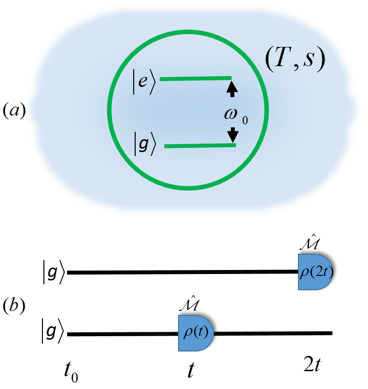
A detailed account of two level systems and their application can be found in Feynman et al. 2011.

We now consider the case when a two level atomic transition $\ket{e}\leftrightarrow\ket{g}$ is driven by an external source. The source is assumed to be a coherent single mode field on resonance. Under dipole approximation, the Hamiltonian (in the interaction picture) is given by $H_{L}=-\vec{E}_{L}(t).\vec{D}(t)$. Here, $\vec{E}_{L}(t)=\vec{\epsilon}e^{-i\omega_{0}t}+\vec{\epsilon}^{*}e^{+i\omega_{0}t}$ is the electric field strength of the driving mode. Also, $\vec{D}(t)=\vec{d}\sigma_{-}e^{-i\omega_{0}t}+\vec{d}^{*}\sigma_{+}e^{+i\omega_{0}t}$ is the atomic dipole operator in the interaction picture and $\vec{d}=\langle g|\vec{D}|e\rangle$ is the transition matrix element of the dipole operator. The atom-field interaction can be written in the rotating wave approximation as follows,

$$H_{L}=-\frac{\Omega}{2}(\sigma_{+}+\sigma_{-}).$$

(6)

Here, $\Omega=2\vec{\epsilon}.\vec{d}^{*}$, is referred to as the Rabi frequency. Now coupling the system to a thermal reservoir leads to the quantum master equation

	$\displaystyle\frac{d\rho(t)}{dt}$	$\displaystyle=\frac{i\Omega}{2}\big[\sigma_{+}+\sigma_{-},\rho(t)\big]$
		$\displaystyle+\gamma_{0}n\bigg(\sigma_{+}\rho(t)\sigma_{-}-\frac{1}{2}\sigma_{-}\sigma_{+}\rho(t)-\frac{1}{2}\rho(t)\sigma_{-}\sigma_{+}\bigg)$
		$\displaystyle+\gamma_{0}(n+1)\bigg(\sigma_{-}\rho(t)\sigma_{+}-\frac{1}{2}\sigma_{+}\sigma_{-}\rho(t)-\frac{1}{2}\rho(t)\sigma_{+}\sigma_{-}\bigg)$
		$\displaystyle-\gamma_{0}M\sigma_{+}\rho(t)\sigma_{+}-\gamma_{0}M^{*}\sigma_{-}\rho(t)\sigma_{-}.$		(7)

Here, $\gamma=\gamma_{0}(2n+1)$ is the total transition rate with $\gamma_{0}$ being the spontaneous emission rate. Further,

	$\displaystyle n$	$\displaystyle=n_{th}(\cosh^{2}(s)+\sinh^{2}(s))+\sinh^{2}(s),$
	$\displaystyle{\rm and}~~M$	$\displaystyle=-\cosh(s)\sinh(s)e^{i\theta}(2n_{th}+1).$		(8)

where $s$ and $\theta$ are the squeezing parameters and $n_{th}=1/(\exp[\beta\omega_{0}]-1)$ is the Plank distribution at transition frequency. In what follows, we will set $\theta=0$ for the purpose of calculations.

In order to solve Eq. (II), we write the density matrix as

$\displaystyle\rho(t)$

$\displaystyle=\frac{1}{2}(\mathbf{I}+\vec{v}(t).\vec{\sigma})=\begin{pmatrix}\frac{1}{2}(1+\langle\sigma_{3}\rangle)&\langle\sigma_{-}\rangle\\ \langle\sigma_{+}\rangle&\frac{1}{2}(1-\langle\sigma_{3}\rangle)\end{pmatrix},$

(9)

with $\vec{v}(t)=\langle\vec{\sigma}(t)\rangle=\operatorname{Tr}[\vec{\sigma}\rho(t)]$, is known as the Bloch vector. With this notation, the master equation, Eq. (II), becomes

$$\frac{d}{dt}\langle\vec{\sigma}(t)\rangle=\mathcal{G}\langle\vec{\sigma}(t)\rangle+\vec{m}.$$

(10)

Here,

$$\mathcal{G}=\begin{pmatrix}-\frac{\gamma}{2}-\gamma_{0}M&0&0\\ \\ 0&-\frac{\gamma}{2}+\gamma_{0}M&\Omega\\ \\ 0&-\Omega&-\gamma\end{pmatrix},$$

(11)

and $\vec{m}=[0~~0~~-\gamma_{0}]^{T}$, $T$ being the transpose operation.

The differential equation (10) has the stationary solution given by

	$\displaystyle\langle\sigma_{3}\rangle_{s}$	$\displaystyle=-\frac{\gamma_{0}(\gamma-2\gamma_{0}M)}{\gamma^{2}-2\gamma\gamma_{0}M+2\Omega^{2}},$
	$\displaystyle\langle\sigma_{+}\rangle_{s}$	$\displaystyle=-\frac{i\gamma_{0}\Omega}{\gamma^{2}-2\gamma\gamma_{0}M+2\Omega^{2}}.$		(12)

Consequently, the stationary population of the excited state $p^{s}_{e}=\frac{1}{2}(1+\langle\sigma_{3}\rangle_{s})=\frac{1}{2}\big[1-\frac{\gamma_{0}(\gamma-2\gamma_{0}M)}{\gamma^{2}-2\gamma\gamma_{0}M+2\Omega^{2}}\big]$.

In the strong driving limit, $\Omega\gg\gamma_{s}$, we have $p_{e}^{s}=1/2$ and $\langle\sigma_{+}\rangle_{s}=-i\gamma_{0}/2\Omega$.

In order to solve the time dependent Bloch equation, Eq. (10), it is convenient to introduce the vector

$$\langle\vec{\Sigma}(t)\rangle=\langle\vec{\sigma}(t)\rangle-\langle\vec{\sigma}\rangle_{s}.$$

(13)

This vector satisfies the homogeneous equation

$$\frac{d}{dt}\langle\vec{\Sigma}(t)\rangle=\mathcal{G}\langle\vec{\Sigma}(t)\rangle.$$

(14)

This equation can be easily solved by diagonalizing $\mathcal{G}$, which has the eigenvalues

	$\displaystyle\lambda_{1}$	$\displaystyle=-\frac{\gamma}{2}-\gamma_{0}M,$
	$\displaystyle\lambda_{2,3}$	$\displaystyle=\frac{\gamma_{0}M}{2}-\frac{3\gamma}{4}\pm i\mu_{s},$		(15)

where,

$$\mu_{s}=\sqrt{\Omega^{2}-\Big(\frac{\gamma_{s}}{4}\Big)^{2}}\quad{\rm with}~~\gamma_{s}=\gamma+2\gamma_{0}M.$$

(16)

Assuming the atom to be initially in the ground state $\rho(0)=\ket{g}\bra{g}$, we have

$$\langle\sigma_{3}(0)\rangle=-1\quad{\rm or}\quad\langle\Sigma_{3}(0)\rangle=-1-\langle\sigma_{3}\rangle_{s},$$

(17)

and

$$\langle\sigma_{\pm}(0)\rangle=0\quad{\rm or}\quad\langle\Sigma_{\pm}(0)\rangle=-\langle\sigma_{\pm}\rangle_{s}.$$

(18)

With these initial conditions, the solution of Eq. (14) is given by

$$\langle\vec{\Sigma}(t)\rangle=\begin{pmatrix}e^{-(\gamma+2\gamma_{0}M)t/2}\langle\Sigma_{1}(0)\rangle\\ \\ e^{(-3\gamma+2\gamma_{0}M)t/4}\Big[\big(\cos(\mu_{s}t)+\frac{\gamma+3\gamma_{0}M}{4\mu_{s}}\sin(\mu_{s}t)\big)\langle\Sigma_{2}(0)\rangle+\frac{\Omega}{\mu_{s}}\sin(\mu_{s}t)\langle\Sigma_{3}(0)\rangle\Big]\\ \\ e^{(-3\gamma+2\gamma_{0}M)t/4}\Big[\big(1-\frac{\gamma_{0}M}{2\mu_{s}}\big)\cos(\mu_{s}t)-\frac{\gamma}{4\mu_{s}}\sin(\mu_{s}t)\Big]\langle\Sigma_{3}(0)\rangle+\frac{i\Omega}{\mu_{s}}e^{(-3\gamma+2\gamma_{0}M)t/4}\sin(\mu_{s}t)\big[\langle\Sigma_{+}(0)\rangle-\langle\Sigma_{-}(0)\rangle\big]\end{pmatrix}.$$

(19)

Having obtained the solution, one can calculate the survival probability of the atom being in the ground state $\ket{g}$, as

$$p_{g}(t)=\frac{1-[\langle\Sigma_{3}(t)\rangle+\langle\sigma_{3}\rangle_{s}]}{2}.$$

(20)

Further, the degree of coherence is proportional to the off-diagonal element

$$\langle\sigma_{+}(t)\rangle=\frac{\langle\sigma_{1}(t)\rangle+i\langle\sigma_{2}(t)\rangle}{2}+\langle\sigma_{+}\rangle_{s}.$$

(21)

The dynamics is underdamped or overdamped depending on whether $\mu_{s}$, defined in Eq. (16), is real or imaginary. As a result, in underdamped regime, the probabilities as well as the coherence exhibit exponentially damped oscillations, while in the over damped case, they monotonically approach to their stationary values, Fig. (2). Throughout this paper, we work in units with $\hbar=k_{B}=1$.

Let $\mathcal{E}_{t_{j}\leftarrow t_{i}}$ be the map corresponding to the evolution given by Eq. (II), such that the system in state $\rho(t_{i})$ at time $t_{i}$ evolves to state $\rho(t_{j})$ at some later time $t_{j}>t_{i}$

$$\rho(t_{j})=\mathcal{E}_{t_{j}\leftarrow t_{i}}[\rho(t_{i})].$$

(22)

Let at time $t_{0}$ the system be in the ground state $\ket{g}$. We define the dichotomic observable $\hat{\mathcal{M}}=|g\rangle\langle g|-|e\rangle\langle e|$. Thus a measurement of this observable leads to $+1$ or $-1$ depending to whether the system is in the ground or excited state, respectively, Fig. (1). We introduce the projectors $\Pi^{+}=|g\rangle\langle g|$ and $\Pi^{-}=|e\rangle\langle e|$, such that $O=\Pi^{+}-\Pi^{-}$. Using Eq. (2), with the notation $t_{1}-t_{0}=t$, the two time correlation $C(t_{0},t_{1})$ is

	$\displaystyle C(t_{0},t_{1})$	$\displaystyle=\operatorname{Tr}[\Pi^{+}\rho(t_{0})]\operatorname{Tr}\Big[\Pi^{+}\mathcal{E}_{t_{1}\leftarrow t_{0}}\big[\frac{\Pi^{+}\rho(t_{0})\Pi^{+}}{\operatorname{Tr}[\Pi^{+}\rho(t_{0})]}\big]\Big]$
		$\displaystyle-\operatorname{Tr}[\Pi^{+}\rho(t_{0})]\operatorname{Tr}\Big[\Pi^{-}\mathcal{E}_{t_{1}\leftarrow t_{0}}\big[\frac{\Pi^{+}\rho(t_{0})\Pi^{+}}{\operatorname{Tr}[\Pi^{+}\rho(t_{0})]}\big]\Big]$
		$\displaystyle-\operatorname{Tr}[\Pi^{-}\rho(t_{0})]\operatorname{Tr}\Big[\Pi^{+}\mathcal{E}_{t_{1}\leftarrow t_{0}}\big[\frac{\Pi^{-}\rho(t_{0})\Pi^{-}}{\operatorname{Tr}[\Pi^{-}\rho(t_{0})]}\big]\Big]$
		$\displaystyle+\operatorname{Tr}[\Pi^{-}\rho(t_{0})]\operatorname{Tr}\Big[\Pi^{-}\mathcal{E}_{t_{1}\leftarrow t_{0}}\big[\frac{\Pi^{-}\rho(t_{0})\Pi^{-}}{\operatorname{Tr}[\Pi^{-}\rho(t_{0})]}\big]\Big],$
		$\displaystyle=p_{g}(t)-p_{e}(t)=2p_{g}(t)-1.$		(23)

Plugging in the expressions of probabilities, we have

$$K_{\pm}=\pm 2\mathcal{F}(t)-\mathcal{F}(2t)\mp 1.$$

(24)

Here,

$$\mathcal{F}(t)=\mathcal{A}\big[\mathcal{B}+\mathcal{C}e^{-(3\gamma-2\gamma_{0}M)t/4}\cos(\mu_{s}t)+\mathcal{D}\sin(\mu_{s}t)\big]-1,$$

(25)

with coefficients given by

	$\displaystyle\mathcal{A}$	$\displaystyle=\big[4\mu_{s}(\gamma^{2}-2\gamma\gamma_{0}M+2\Omega^{2})\big]^{-1},$
	$\displaystyle\mathcal{B}$	$\displaystyle=4(\gamma+\gamma_{0})(\gamma-2\gamma_{0}M)\mu_{s}+8\mu_{s}\Omega^{2},$
	$\displaystyle\mathcal{C}$	$\displaystyle=-2(\gamma_{0}M-2\mu_{s})\big[(\gamma-\gamma_{0})(\gamma-2\gamma_{0}M)+2\Omega^{2}\big],$
	$\displaystyle\mathcal{D}$	$\displaystyle=-\gamma(\gamma-\gamma_{0})(\gamma-2\gamma_{0}M)-2(\gamma-4\gamma_{0})\Omega^{2}.$		(26)

In the strong driving limit, $\Omega\gg\gamma_{s}$, the coefficients can be approximated as $\mathcal{A}\approx\Omega^{-3}$, $\mathcal{B}\approx\mathcal{C}\approx\Omega^{3}$ and $\mathcal{D}\approx\Omega^{2}$, such that in this limit, $\mathcal{F}(t)\propto\cos(\Omega t)$ and therefore

$$K_{\pm}\approx\pm 2\cos(\Omega t)-\cos(2\Omega t).$$

(27)

Effect of weak measurement: The two time correlation function $C(t_{0},t)$, Eq. (III), was obtained by assuming that the measurements are ideal or projective. However, it would be interesting to see how weak measurements affect the behavior of $C(t_{0},t)$ and thereby of the LG parameters $K_{\pm}$. The weak measurements are characterized by invoking a parameter $\xi$ Busch 1986; Saha et al. 2015, such that the ideal projectors $\Pi^{\pm}$ are replaced by the “weak projectors” $W^{\pm}$ defined as

$$W^{\pm}=\Big(\frac{1\pm\xi}{2}\Big)\Pi^{+}+\Big(\frac{1\mp\xi}{2}\Big)\Pi^{-}.$$

(28)

Here, $0<\xi\leq 1$, such that when $\xi=1$, $W^{\pm}$ reduce to the ideal projection operators $\Pi^{\pm}$. Invoking weak projectors leads to the following form of the two time correlation function becomes $C(t_{0},t)|_{weak}=\xi^{2}C(t_{0},t)$, and consequently

$$K_{\pm}|_{weak}=\xi^{2}K_{\pm}.$$

(29)

Therefore, the maximum violation of LGtI occurs for an ideal projective measurement.

The LGtIs given by inequality (3) are studied in the context of a two level atom with the ground and excited states labelled as $\ket{g}$ and $\ket{e}$, respectively. An external field is driving the transition between the two levels. Further, the atom is allowed to interact with a squeezed thermal bath. The inequalities thus obtained are in terms of experimentally relevant parameters. The violation of LGtIs occur predominantly in the underdamped regime which is characterized by the real values of parameter $\mu_{s}$ defined in Eq. (16), such that

	$\displaystyle\Omega$	$\displaystyle>\frac{\gamma_{s}}{4}=\gamma_{0}\frac{(2n+1)+2M}{4}~~~{\rm underdamped},$
	$\displaystyle\Omega$	$\displaystyle<\frac{\gamma_{s}}{4}=\gamma_{0}\frac{(2n+1)+2M}{4}~~~{\rm overdamped}.$		(30)

Figure (3) depicts the behavior of LG parameters $K_{\pm}$ with respect to time $t$, for different values of the ratio $R=\gamma_{0}/\Omega$. The violations of LGtIs are observed mainly in the underdamped regime and fade quickly with the increase in $R$. In other words, strong driving favors the violation of LGtIs to their maximum quantum bound. The right most panel of the figure shows coherence paramter $C$ Alok et al. 2016; Bhattacharya et al. 2018 which is defined as

$$C=\sum\limits_{i\neq j}|\rho_{ij}|.$$

(31)

The extent of violation of LGtIs can be seen as a signature of the degree of coherence in the system.

In the strong driving limit, i.e., $\Omega\gg\gamma_{s}$, the LG parameters are given by Eq. (27) and are plotted in Fig. (4). The parameters $K_{+}$ and $K_{-}$ show complementary behavior in the sense that when one of these parameters does not show a violation, the other does, together covering the entire parameter range.

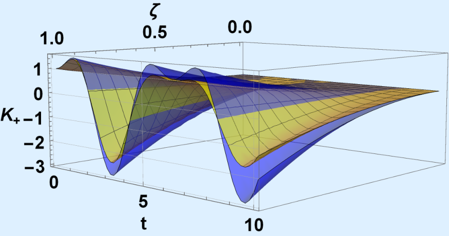
The interaction with the squeezed thermal reservoir leads to enhancement in the transition rate which is given by $\gamma=\gamma_{0}(2n+1)$, where $\gamma_{0}$ is the spontaneous emission rate and $\gamma_{0}n$ is the squeezed thermal induced emission and absorption rate. The interactions with the reservoir are expected to decrease the quantumness in the system. This feature is depicted in Fig. (5), where $K_{+}$ shows enhanced violations for larger values of the parameter $\beta$ i.e, for smaller temperature.

The squeezing parameter as defined in Eq. (II), controls the degree of violation of LGtIs, since it affects the total photon distribution. Figure (6) exhibits the variation of the LG parameter $K_{+}$ for different values of squeezing parameter $s$. The increase in $s$ is found to decrease the extent of violation of LGtI.

The effect of weak measurement on the LG parameters is depicted in Fig. (7). The ideal projective measurements are characterized by $\xi=1$, while $\xi=0$ corresponds to no measurement. It is clear from the figure that the maximum violation occurs for ideal projective measurements.

We studied the violation of Leggett-Garg type inequalities in a driven two level atom interacting with a squeezed thermal bath. The effect of various experimentally relevant parameters on the violation of the inequality were examined carefully. The violations were seen to be prominent in the underdamped case. The increase in temperature was found to decrease the degree of violation as well as the time over which the violation is sustained. Squeezing the thermal state of the reservoir was also found to reduce the violation of LGtIs. Enhanced violations, reaching to the quantum bound, were witnessed in the strong driving limit. Further, we studied the effect of the weak measurements on the extent of violation of LGtI. The weak measurements are characterized by the parameter $\xi$ such that $\xi=0$ ($\xi=1$) corresponds to no measurement (ideal projective measurement). The maximum violation was found to occur for the ideal projective measurements.

AMJ thanks DST India for J C Bose National Fellowship.

References

- Schrödinger (1935) E. Schrödinger, Naturwissenschaften 23, 823 (1935).
- Einstein et al. (1935) A. Einstein, B. Podolsky, and N. Rosen, Phys. Rev. 47, 777 (1935).
- Bell (1964) J. S. Bell, Physics Physique Fizika 1, 195 (1964).
- Horodecki et al. (2009) R. Horodecki, P. Horodecki, M. Horodecki, and K. Horodecki, Reviews of Modern Physics 81, 865 (2009).
- Leggett and Garg (1985) A. J. Leggett and A. Garg, Physical Review Letters 54, 857 (1985).
- Emary et al. (2013) C. Emary, N. Lambert, and F. Nori, Reports on Progress in Physics 77, 016001 (2013).
- Chakrabarty et al. (2011) I. Chakrabarty, S. Banerjee, and N. Siddharth, Quantum Info. Comput. 11, 541 (2011).
- Barbieri (2009) M. Barbieri, Physical Review A 80, 034102 (2009).
- Avis et al. (2010) D. Avis, P. Hayden, and M. M. Wilde, Physical Review A 82, 030102 (2010).
- Lambert et al. (2010) N. Lambert, C. Emary, Y.-N. Chen, and F. Nori, Physical Review Letters 105, 176801 (2010).
- Lambert et al. (2011) N. Lambert, R. Johansson, and F. Nori, Physical Review B 84, 245421 (2011).
- Montina (2012) A. Montina, Physical Review Letters 108, 160501 (2012).
- Kofler and Brukner (2013) J. Kofler and Č. Brukner, Physical Review A 87, 052115 (2013).
- Budroni et al. (2013) C. Budroni, T. Moroder, M. Kleinmann, and O. Gühne, Physical Review Letters 111, 020403 (2013).
- Kumari and Pan (2017) S. Kumari and A. Pan, EPL (Europhysics Letters) 118, 50002 (2017).
- Naikoo et al. (2018a) J. Naikoo, A. K. Alok, and S. Banerjee, Phys. Rev. D 97, 053008 (2018a).
- Naikoo et al. (2019) J. Naikoo, A. K. Alok, S. Banerjee, and S. U. Sankar, Phys. Rev. D 99, 095001 (2019).
- Naikoo et al. (2018b) J. Naikoo, S. Banerjee, and R. Srikanth, arXiv preprint arXiv:1806.00537 (2018b).
- Naikoo and Banerjee (2018) J. Naikoo and S. Banerjee, The European Physical Journal C 78, 602 (2018).
- Palacios-Laloy et al. (2010) A. Palacios-Laloy, F. Mallet, F. Nguyen, P. Bertet, D. Vion, D. Esteve, and A. N. Korotkov, Nature Physics 6, 442 (2010).
- Groen et al. (2013) J. Groen, D. Ristè, L. Tornberg, J. Cramer, P. C. De Groot, T. Picot, G. Johansson, and L. DiCarlo, Physical Review Letters 111, 090506 (2013).
- Goggin et al. (2011) M. Goggin, M. Almeida, M. Barbieri, B. Lanyon, J. O’Brien, A. White, and G. Pryde, Proceedings of the National Academy of Sciences 108, 1256 (2011).
- Dressel et al. (2011) J. Dressel, C. Broadbent, J. Howell, and A. N. Jordan, Physical Review Letters 106, 040402 (2011).
- Suzuki et al. (2012) Y. Suzuki, M. Iinuma, and H. F. Hofmann, New Journal of Physics 14, 103022 (2012).
- Athalye et al. (2011) V. Athalye, S. S. Roy, and T. Mahesh, Physical Review Letters 107, 130402 (2011).
- Souza et al. (2011) A. Souza, I. Oliveira, and R. Sarthour, New Journal of Physics 13, 053023 (2011).
- Katiyar et al. (2013) H. Katiyar, A. Shukla, K. R. K. Rao, and T. Mahesh, Physical Review A 87, 052102 (2013).
- Huelga et al. (1995) S. F. Huelga, T. W. Marshall, and E. Santos, Phys. Rev. A 52, R2497 (1995).
- Huelga et al. (1996) S. F. Huelga, T. W. Marshall, and E. Santos, Phys. Rev. A 54, 1798 (1996).
- Waldherr et al. (2011) G. Waldherr, P. Neumann, S. F. Huelga, F. Jelezko, and J. Wrachtrup, Phys. Rev. Lett. 107, 090401 (2011).
- Xu et al. (2011) J.-S. Xu, C.-F. Li, X.-B. Zou, and G.-C. Guo, Scientific reports 1, 101 (2011).
- Zhou et al. (2015) Z.-Q. Zhou, S. F. Huelga, C.-F. Li, and G.-C. Guo, Phys. Rev. Lett. 115, 113002 (2015).
- Srikanth and Banerjee (2008) R. Srikanth and S. Banerjee, Phys. Rev. A 77, 012318 (2008).
- Banerjee and Srikanth (2008) S. Banerjee and R. Srikanth, The European Physical Journal D 46, 335 (2008).
- Breuer et al. (2002) H.-P. Breuer, F. Petruccione, et al., The theory of open quantum systems (Oxford University Press on Demand, 2002).
- Banerjee (2018) S. Banerjee, Open Quantum Systems: Dynamics of Nonclassical Evolution, Vol. 20 (Springer, 2018).
- Omkar et al. (2013) S. Omkar, R. Srikanth, and S. Banerjee, Quantum Information Processing 12, 3725 (2013).
- Feynman et al. (2011) R. Feynman, R. Leighton, and M. Sands, The Feynman Lectures on Physics, Vol. III: The New Millennium Edition: Quantum Mechanics, The Feynman Lectures on Physics (Basic Books, 2011).
- Busch (1986) P. Busch, Phys. Rev. D 33, 2253 (1986).
- Saha et al. (2015) D. Saha, S. Mal, P. K. Panigrahi, and D. Home, Phys. Rev. A 91, 032117 (2015).
- Alok et al. (2016) A. K. Alok, S. Banerjee, and S. U. Sankar, Nuclear Physics B 909, 65 (2016).
- Bhattacharya et al. (2018) S. Bhattacharya, S. Banerjee, and A. K. Pati, Quantum Information Processing 17, 236 (2018).