跳到论文正文
W Papers独立论文阅读器 arXiv:1908.04050 论文正文 计算阅读时间 · 0%
引用这篇论文根据当前论文元数据生成,正式投稿前建议核对。


License: arXiv.org perpetual non-exclusive license
arXiv:1908.04050v1 [math.AP] 12 Aug 2019

The Bilinear Strategy for Calderón’s Problem

Felipe Ponce-Vanegas Affiliation: BCAM - Basque Center for Applied Mathematics Affiliation: fponce@bcamath.org
Abstract

Electrical Impedance Imaging would suffer a serious obstruction if for two different conductivities the potential and current measured at the boundary were the same. The Calderón’s problem is to decide whether the conductivity is indeed uniquely determined by the data at the boundary. In ℝd\mathbb{R}^{d}, for d=5,6d=5,6, we show that uniqueness holds when the conductivity is in W1+d−52​p+,p​(Ω)W^{1+\frac{d-5}{2p}+,p}(\Omega), for d≤p<∞d\leq p<\infty. This improves on recent results of Haberman, and of Ham, Kwon and Lee. The main novelty of the proof is an extension of Tao’s bilinear Theorem.

1 Introduction

Electrical Impedance Imaging is a technique to reconstruct the inner structure of a body from measurements of potential and current at the boundary. At least since the 30’, geophysicists have used this technique to identify different layers of earth underground [22]. In pioneering work, Calderón [7] posed the problem of deciding whether the conductivity is uniquely determined by measurements at the boundary. Calderón went on to show uniqueness, roughly, when the conductivity is close to one.

The electrical potential uu in a bounded domain Ω⊂ℝd\Omega\subset\mathbb{R}^{d} with Lipschitz boundary satisfies the differential equation

Lγ​u\displaystyle L_{\gamma}u :=div(γ∇u)=0,\displaystyle:=\text{div}\,(\gamma\nabla u)=0, (1)
u|∂Ω\displaystyle u|_{\partial\Omega} =f,\displaystyle=f,

where γ\gamma is the conductivity and ff the potential at the boundary. We assume that γ∈L∞​(Ω)\gamma\in L^{\infty}(\Omega) and that γ≥c>0\gamma\geq c>0. If f∈H1/2​(∂Ω)f\in H^{1/2}(\partial\Omega), then a solution u∈H1​(Ω)u\in H^{1}(\Omega) exists. The electrical current at the boundary is γ​∂νu∣∂Ω\gamma\partial_{\nu}u\mid_{\partial\Omega}, where ν\nu is the outward-pointing normal, and the operator Λγ:u|∂Ω↦γ​∂νu∣∂Ω\Lambda_{\gamma}:u|_{\partial\Omega}\mapsto\gamma\partial_{\nu}u\mid_{\partial\Omega} is called the Dirichlet-to-Neumann map; we can define the map Λγ\Lambda_{\gamma} rigorously as

⟨Λγf,g⟩:=∫Ωγ∇u⋅∇v¯,\langle\Lambda_{\gamma}f,g\rangle:=\int_{\Omega}\gamma\nabla u\cdot\nabla\bar{v}, (2)

where uu solves (1) and v∈H1​(Ω)v\in H^{1}(\Omega) is any extension of g∈H1/2​(∂Ω)g\in H^{1/2}(\partial\Omega); hence Λγ:H1/2(∂Ω)↦H−1/2(∂Ω)\Lambda_{\gamma}:H^{1/2}(\partial\Omega)\mapsto H^{-1/2}(\partial\Omega). If we choose vv such that Lγ​v=0L_{\gamma}v=0, then we see that Λγ\Lambda_{\gamma} is symmetric. Uniqueness fails if two different conductivities γ1\gamma_{1} and γ2\gamma_{2} satisfy Λγ1=Λγ2\Lambda_{\gamma_{1}}=\Lambda_{\gamma_{2}}; this were the case, for every f1,f2∈H12​(∂Ω)f_{1},f_{2}\in H^{\frac{1}{2}}(\partial\Omega) we would have

0=⟨(Λγ1−Λγ2)f1,f2⟩=∫Ω(γ1−γ2)∇u1⋅∇u¯2,0=\langle(\Lambda_{\gamma_{1}}-\Lambda_{\gamma_{2}})f_{1},f_{2}\rangle=\int_{\Omega}(\gamma_{1}-\gamma_{2})\nabla u_{1}\cdot\nabla\overline{u}\,_{2}, (3)

where Lγ1​u1=0L_{\gamma_{1}}u_{1}=0 and Lγ2​u2=0L_{\gamma_{2}}u_{2}=0 are extensions of f1f_{1} and f2f_{2} respectively. Most of the proofs of uniqueness show that the collection of functions {∇u1⋅∇u¯2}\{\nabla u_{1}\cdot\nabla\overline{u}\,_{2}\} is dense, so γ1\gamma_{1} and γ2\gamma_{2} cannot be different.

Kohn and Vogelius [16] showed that for smooth conductivities γ1\gamma_{1} and γ2\gamma_{2}, uniqueness holds at the boundary to all orders, so ∂νNγ1=∂νNγ2\partial_{\nu}^{N}\gamma_{1}=\partial_{\nu}^{N}\gamma_{2} at ∂Ω\partial\Omega for every integer NN. In particular, if the conductivities are analytic, then γ1=γ2\gamma_{1}=\gamma_{2} in Ω\Omega.

In [24], Sylvester and Uhlmann introduced the method that most of the proofs follow nowadays. If uju_{j} solve the equation (1) for γj\gamma_{j}, then the function wj:=γj12​uiw_{j}:=\gamma_{j}^{\frac{1}{2}}u_{i} solves the equation (−Δ+qj)​wj=0(-\Delta+q_{j})w_{j}=0 with qj=γj−12​Δ​γj12q_{j}=\gamma_{j}^{-\frac{1}{2}}\Delta\gamma_{j}^{\frac{1}{2}}, and the relationship (3) is replaced by

∫ℝd(q1−q2)​w1​w2=0;\int_{\mathbb{R}^{d}}(q_{1}-q_{2})w_{1}w_{2}=0; (4)

then, they had to prove that the collection of function {w1​w2}\{w_{1}w_{2}\} is dense. The integral is evaluated over ℝd\mathbb{R}^{d} because the functions γ1\gamma_{1} and γ2\gamma_{2} are extended to the whole space, and are arranged so that γ1=γ2=1\gamma_{1}=\gamma_{2}=1 outside a ball containing Ω\Omega. Since eζ⋅xe^{\zeta\cdot x} is harmonic when ζ∈ℂd\zeta\in\mathbb{C}^{d} satisfies ζ⋅ζ=0\zeta\cdot\zeta=0, then they used the ansatz wj=eζj⋅x​(1+ψj)w_{j}=e^{\zeta_{j}\cdot x}(1+\psi_{j}), expecting that ψj\psi_{j} is somehow negligible for |ζ1|,|ζ2|→∞\lvert\zeta_{1}\rvert,\lvert\zeta_{2}\rvert\to\infty. These solutions wjw_{j} are called Complex Geometrical Optics (CGO) solutions. Sylvester and Uhlmann selected ζ1\zeta_{1} and ζ2\zeta_{2} such that ζ1+ζ2=i​ξ\zeta_{1}+\zeta_{2}=i\xi for ξ∈ℝd\xi\in\mathbb{R}^{d}; then, on the assumed smallness of ψj\psi_{j} for |ζ1|,|ζ2|→∞\lvert\zeta_{1}\rvert,\lvert\zeta_{2}\rvert\to\infty, equation (4) means that q^1=q^2\widehat{q}_{1}=\widehat{q}_{2}, and this implies that γ1=γ2\gamma_{1}=\gamma_{2}. Their argument works well for conductivities in C2​(Ω)C^{2}(\Omega).

In ℝ2\mathbb{R}^{2}, Astala and Päivärinta [1] proved that uniqueness holds in L∞​(Ω)L^{\infty}(\Omega), the best possible result. In higher dimensions, Brown [4] proved uniqueness for conductivities in C32+​(Ω)C^{\frac{3}{2}+}(\Omega), and this was improved to W32,2​d+​(Ω)W^{\frac{3}{2},2d+}(\Omega) by Brown and Torres [6]. By analogy with unique continuation, it is conjectured that the lowest possible regularity is W1,d​(Ω)W^{1,d}(\Omega).

The function ψ\psi in the CGO solution w=eζ⋅x​(1+ψ)w=e^{\zeta\cdot x}(1+\psi) satisfies the equation

Δζ​ψ:=Δ​ψ+2​ζ⋅∇ψ=q⁡(1+ψ).\Delta_{\zeta}\psi:=\Delta\psi+2\zeta\cdot\nabla\psi=q(1+\psi). (5)

Then, it is necessary to prove that a solution exists and is small. In [12], Haberman and Tataru introduced a Bourgain-type space adapted to pζ​(ξ)=−|ξ|2+2​i​ζ⋅ξp_{\zeta}(\xi)=-\lvert\xi\rvert^{2}+2i\zeta\cdot\xi, the symbol of Δζ\Delta_{\zeta}. The space is defined as

X˙ζb:={u∣∥u∥X˙ζb2:=∫ℝd|pζ​(ξ)|2​b​|u^|2​𝑑ξ<∞},\dot{X}^{b}_{\zeta}:=\{u\mid\lVert u\rVert_{\dot{X}^{b}_{\zeta}}^{2}:=\int_{\mathbb{R}^{d}}\lvert p_{\zeta}(\xi)\rvert^{2b}\lvert\widehat{u}\rvert^{2}\,d\xi<\infty\},

and it follows immediately that ∥Δζ−1∥X˙ζ−12→X˙ζ12=1\lVert\Delta_{\zeta}^{-1}\rVert_{\dot{X}^{-\frac{1}{2}}_{\zeta}\to\dot{X}^{\frac{1}{2}}_{\zeta}}=1. The dual of X˙ζb\dot{X}^{b}_{\zeta} is X˙ζ−b\dot{X}^{-b}_{\zeta}. If we define the multiplication operator Mq:u↦q​uM_{q}:u\mapsto qu, then the existence of ψ\psi follows from ∥Δζ−1​Mq∥X˙ζ12→X˙ζ12≤∥Mq∥X˙ζ12→X˙ζ−12≤c<1\lVert\Delta^{-1}_{\zeta}M_{q}\rVert_{\dot{X}^{\frac{1}{2}}_{\zeta}\to\dot{X}^{\frac{1}{2}}_{\zeta}}\leq\lVert M_{q}\rVert_{\dot{X}^{\frac{1}{2}}_{\zeta}\to\dot{X}^{-\frac{1}{2}}_{\zeta}}\leq c<1, and the smallness of ψ\psi follows from the smallness of ∥q∥X˙ζ−12\lVert q\rVert_{\dot{X}^{-\frac{1}{2}}_{\zeta}}. Using these spaces Haberman and Tataru proved uniqueness for Lipschitz conductivities close to one.

Caro and Rogers [8] proved uniqueness for Lipschitz conductivities without further restriction. They used Carleman estimates, in the spirit of [15] and [9].

After an observation in [21], Haberman refined in [11] the method of Bourgain spaces, and proved uniqueness for conductivities in W1,3​(Ω)W^{1,3}(\Omega) for d=3d=3, and W1+d−42​p,p​(Ω)W^{1+\frac{d-4}{2p},p}(\Omega) for p≥dp\geq d and d=4,5,6d=4,5,6. He argued as follows: for γ1\gamma_{1} and γ2\gamma_{2} he wanted to show that ∥Mqj∥X˙ζj12→X˙ζj−12\lVert M_{q_{j}}\rVert_{\dot{X}^{\frac{1}{2}}_{\zeta_{j}}\to\dot{X}^{-\frac{1}{2}}_{\zeta_{j}}} and ∥qj∥X˙ζj−12\lVert q_{j}\rVert_{\dot{X}^{-\frac{1}{2}}_{\zeta_{j}}} are small for some ζ1\zeta_{1} and ζ2\zeta_{2} that satisfy ζ1+ζ2=i​ξ\zeta_{1}+\zeta_{2}=i\xi, so Haberman proved that there exist sequences {ζ1,k}\{\zeta_{1,k}\} and {ζ2,k}\{\zeta_{2,k}\} for which ∥Mqj∥X˙ζj,k12→X˙ζj,k−12\lVert M_{q_{j}}\rVert_{\dot{X}^{\frac{1}{2}}_{\zeta_{j,k}}\to\dot{X}^{-\frac{1}{2}}_{\zeta_{j,k}}} and ∥qj∥X˙ζj,k−12\lVert q_{j}\rVert_{\dot{X}^{-\frac{1}{2}}_{\zeta_{j,k}}} tend to zero as |ζ1,k|,|ζ2,k|→∞\lvert\zeta_{1,k}\rvert,\lvert\zeta_{2,k}\rvert\to\infty. To find the sequences, he proved that the expected value of both norms goes to zero as |ζ1|,|ζ2|→∞\lvert\zeta_{1}\rvert,\lvert\zeta_{2}\rvert\to\infty.

Theorem 1 (Haberman [11]).

Let us write ζ⁡(U,τ):=τ⁡(U​e1−i​U​e2)\zeta(U,\tau):=\tau(Ue_{1}-iUe_{2}) for τ≥1\tau\geq 1 and U∈OdU\in O_{d} a rotation. If ∇log⁡γ1\nabla\log\gamma_{1} and ∇log⁡γ2\nabla\log\gamma_{2} are in Wd−42​p,p​(ℝd)W^{\frac{d-4}{2p},p}(\mathbb{R}^{d}) for d≤p<∞d\leq p<\infty, or in L3​(ℝd)L^{3}(\mathbb{R}^{d}) for d=3d=3, then

1M​∫M2​M∫Od∥Mqj∥X˙ζ⁡(U,τ)12→X˙ζ⁡(U,τ)−12p​𝑑U​𝑑τ​ and ​1M​∫M2​M∫Od∥qj∥X˙ζ⁡(U,τ)−122​𝑑U​𝑑τ→M→∞0.\frac{1}{M}\int\limits_{M}^{2M}\int\limits_{O_{d}}\lVert M_{q_{j}}\rVert_{\dot{X}^{\frac{1}{2}}_{\zeta(U,\tau)}\to\dot{X}^{-\frac{1}{2}}_{\zeta(U,\tau)}}^{p}\,dUd\tau\text{ and }\frac{1}{M}\int\limits_{M}^{2M}\int\limits_{O_{d}}\lVert q_{j}\rVert_{\dot{X}^{-\frac{1}{2}}_{\zeta(U,\tau)}}^{2}\,dUd\tau\xrightarrow{M\to\infty}0.

The idea is that, when |ζj|\lvert\zeta_{j}\rvert is large, the set of bad pairs (ζ1,ζ2)(\zeta_{1},\zeta_{2}) for which ∥Mqj∥X˙ζj,k12→X˙ζj,k−12\lVert M_{q_{j}}\rVert_{\dot{X}^{\frac{1}{2}}_{\zeta_{j,k}}\to\dot{X}^{-\frac{1}{2}}_{\zeta_{j,k}}} or ∥qj∥X˙ζj,k−12\lVert q_{j}\rVert_{\dot{X}^{-\frac{1}{2}}_{\zeta_{j,k}}} is large has measure close to zero, then it is possible to extract sequences such that these norms are small and such that ζ1+ζ2=i​ξ\zeta_{1}+\zeta_{2}=i\xi.

The estimates of Haberman are very good, and most of the argument works well just for γ∈W1,d​(Ω)\gamma\in W^{1,d}(\Omega). The bottle-neck is to get a strong upper bound of ∥M∂if∥X˙ζ⁡(U,τ)12→X˙ζ⁡(U,τ)−12\lVert M_{\partial_{i}f}\rVert_{\dot{X}^{\frac{1}{2}}_{\zeta(U,\tau)}\to\dot{X}^{-\frac{1}{2}}_{\zeta(U,\tau)}}, where f∈Ws,pf\in W^{s,p} for some s≥0s\geq 0.

In Section 2 we proof the next theorem.

Theorem 2 (Vanishing of the Expected Value).

Let us write ζ⁡(U,τ):=τ⁡(U​e1−i​U​e2)\zeta(U,\tau):=\tau(Ue_{1}-iUe_{2}) for τ≥1\tau\geq 1 and U∈OdU\in O_{d} a rotation. Suppose that ff is a function supported in the unit ball. If f∈Wd−52​p+,p​(ℝd)f\in W^{\frac{d-5}{2p}+,p}(\mathbb{R}^{d}) for d≤p<∞d\leq p<\infty, then

1M​∫M2​M∫Od∥M∂if∥X˙ζ⁡(U,τ)12→X˙ζ⁡(U,τ)−12​𝑑U​𝑑τ→M→∞0.\frac{1}{M}\int\limits_{M}^{2M}\int\limits_{O_{d}}\lVert M_{\partial_{i}f}\rVert_{\dot{X}^{\frac{1}{2}}_{\zeta(U,\tau)}\to\dot{X}^{-\frac{1}{2}}_{\zeta(U,\tau)}}\,dUd\tau\xrightarrow{M\to\infty}0. (6)

The main consequence of this theorem is the next improvement on Calderón’s problem.

Theorem 3.

For d=5,6d=5,6 suppose that Ω⊂ℝd\Omega\subset\mathbb{R}^{d} is a bounded domain with Lipschitz boundary. If γ1\gamma_{1} and γ2\gamma_{2} are in W1+d−52​p+,p​(Ω)∩L∞W^{1+\frac{d-5}{2p}+,p}(\Omega)\cap L^{\infty} for d≤p<∞d\leq p<\infty, and if γ1,γ2≥c>0\gamma_{1},\gamma_{2}\geq c>0, then

Λγ1=Λγ2​ implies ​γ1=γ2.\Lambda_{\gamma_{1}}=\Lambda_{\gamma_{2}}\kern 5.0pt\text{ implies }\kern 5.0pt\gamma_{1}=\gamma_{2}.

We write γ∈W1+d−52​p+,p​(Ω)∩L∞\gamma\in W^{1+\frac{d-5}{2p}+,p}(\Omega)\cap L^{\infty} to emphasize that γ∈L∞\gamma\in L^{\infty}, but it follows from Sobolev embedding for domains with Lipschitz boundaries. We note that Theorem 2 holds for d≥3d\geq 3, and the restriction d=5,6d=5,6 in Theorem 3 seems technical; in fact, we can state the following consequence of the vanishing of the expected value.

Theorem 4.

For d≥7d\geq 7 suppose that Ω⊂ℝd\Omega\subset\mathbb{R}^{d} is a bounded domain with Lipschitz boundary. If γ1\gamma_{1} and γ2\gamma_{2} are in W1+d−52​p+,p​(Ω)∩L∞W^{1+\frac{d-5}{2p}+,p}(\Omega)\cap L^{\infty} for d≤p<∞d\leq p<\infty, if ∂νγ1=∂νγ2\partial_{\nu}\gamma_{1}=\partial_{\nu}\gamma_{2} at ∂Ω\partial\Omega, and if γ1,γ2≥c>0\gamma_{1},\gamma_{2}\geq c>0, then

Λγ1=Λγ2​ implies ​γ1=γ2.\Lambda_{\gamma_{1}}=\Lambda_{\gamma_{2}}\kern 5.0pt\text{ implies }\kern 5.0pt\gamma_{1}=\gamma_{2}.

By the trace theorem the normal derivative ∂νγ\partial_{\nu}\gamma is well-defined. The proof of Theorem 3 and Theorem 4 has been already summarized in this introduction, and we provide some more details in Section 2. We refer the reader to the literature to reconstruct the whole argument, in particular to Haberman [11] and to Ham, Kwon and Lee [13].

1.1 Restriction Theory

Ham, Kwon and Lee [13] applied deep estimates from restriction theory to improve on Harberman results, and we will follow most of their arguments. We give here a brief introduction to restriction theory and the way it comes in Calderón’s problem; a detailed exposition of restriction theory can be found in [20, part IV].

We control the norm ∥M∂if∥X˙ζ⁡(U,τ)12→X˙ζ⁡(U,τ)−12\lVert M_{\partial_{i}f}\rVert_{\dot{X}^{\frac{1}{2}}_{\zeta(U,\tau)}\to\dot{X}^{-\frac{1}{2}}_{\zeta(U,\tau)}} by duality, so we need an upper bound of

⟨(∂if)​u,v⟩=∫ℝd(∂if)​u​v¯​𝑑xfor ​u,v∈X˙ζ⁡(U,τ)12.\langle(\partial_{i}f)u,v\rangle=\int_{\mathbb{R}^{d}}(\partial_{i}f)u\overline{v}\,\,dx\quad\text{for }u,v\in\dot{X}^{\frac{1}{2}}_{\zeta(U,\tau)}. (7)

The contribution coming from frequencies close the null set of pζ​(ξ)=−|ξ|2+2​i​ζ⋅ξp_{\zeta}(\xi)=-\lvert\xi\rvert^{2}+2i\zeta\cdot\xi, which we call the characteristic set Σζ\Sigma_{\zeta}, is the hardest part we have to deal with.

The characteristic set Σζ\Sigma_{\zeta} is a (d−2)(d-2)-sphere, and we have to control the duality pairing when the Fourier transform of uu and vv is concentrated close to Σζ\Sigma_{\zeta}. This is just the setting for which restriction theory has been developed; a few classical examples of applications are [10, 14, 2, 3].

In restriction theory, we seek to prove the best possible bounds ∥f^∣S∥p≤C​∥f∥q\lVert\widehat{f}\mid_{S}\rVert_{p}\leq C\lVert f\rVert_{q}, where SS is a manifold or just a set. One of earliest and most important result is due to Tomas [27] and Stein (unpublished); for the proof see e.g. [23, chp. 9].

Theorem 5.

(Tomas-Stein Inequality) Suppose that S⊂ℝnS\subset\mathbb{R}^{n} is a compact surface with non-vanishing curvature. If f∈Lp​(ℝn)f\in L^{p}(\mathbb{R}^{n}) for 1≤p≤2​n+1n+31\leq p\leq 2\frac{n+1}{n+3}, then

∥f^∣S∥2≤C​∥f∥p.\lVert\widehat{f}\mid_{S}\rVert_{2}\leq C\lVert f\rVert_{p}. (8)

The dual operator is called the extension operator, and it is the Fourier transform of a measure f​d​SfdS supported on the set SS. The function (f​d​S)∨(fdS)^{\vee} is the prototype of a function with frequencies highly concentrated close to SS. In the dual side, the Tomas-Stein inequality is

∥(f​d​S)∨∥Lp′​(ℝn)≤C​∥f∥L2​(S)for ​ 2​n+1n−1≤p′≤∞.\lVert(fdS)^{\vee}\rVert_{L^{p^{\prime}}(\mathbb{R}^{n})}\leq C\lVert f\rVert_{L^{2}(S)}\quad\text{for }\,2\frac{n+1}{n-1}\leq p^{\prime}\leq\infty. (9)

Since the earliest days of restriction theory, a kind of stability of bilinear estimates was exploited; for example, the bound ∥(f​d​S)∨∥L4​(ℝ2)≤C​∥f∥2\lVert(fdS)^{\vee}\rVert_{L^{4}(\mathbb{R}^{2})}\leq C\lVert f\rVert_{2} is false, but the bound ∥(f1​d​S1)∨​(f2​d​S2)∨∥L2​(ℝ2)≤C​∥f1∥2​∥f2∥2\lVert(f_{1}dS_{1})^{\vee}(f_{2}dS_{2})^{\vee}\rVert_{L^{2}(\mathbb{R}^{2})}\leq C\lVert f_{1}\rVert_{2}\lVert f_{2}\rVert_{2} is true, whenever the lines S1S_{1} and S2S_{2} are transversal; curvature is not required. This stability of bilinear estimates was clarified and refined by Tao, Vargas and Vega [26].

If we are to expect some improvement of a bilinear estimate, we have to require a separation condition on the surfaces S1S_{1} and S2S_{2} involved. For example, if ∥(f1​d​S1)∨​(f2​d​S2)∨∥L2​(ℝ2)≤C​∥f1∥2​∥f2∥2\lVert(f_{1}dS_{1})^{\vee}(f_{2}dS_{2})^{\vee}\rVert_{L^{2}(\mathbb{R}^{2})}\leq C\lVert f_{1}\rVert_{2}\lVert f_{2}\rVert_{2} were true in any case, then just setting S1=S2S_{1}=S_{2} would provide a linear estimate, a false one in this case. One of the key outcomes of [26] is a general strategy to get linear bounds from bilinear bounds, and we will follow this strategy in Section 3.1.

If we are to use the bilinear strategy, we need strong bilinear upper bounds. For some time, the bilinear analogue of the Tomas-Stein inequality in ℝn\mathbb{R}^{n}, for n≥3n\geq 3, was known as Klainerman-Machedon conjecture. Wolff made the first big progress, proving the conjecture when the surfaces are subsets of the cone [30]. Subsequently, Tao refined the method and proved the conjecture when the surfaces are subsets of a surface with positive curvature [25]. Vargas [29] and Lee [18] proved the conjecture when the surfaces are subsets of the hyperboloid, dealing with unusual obstructions.

Since we are interested in the sphere, we need to prove the bilinear theorem for this case. To avoid antipodal points in the bilinear inequality, we restrict ourselves to the surface

S:={(ξ′,ξn)∣ξn=1−1−|ξ′|2​ and ​|ξ′|<12+110}S:=\{(\xi^{\prime},\xi_{n})\mid\xi_{n}=1-\sqrt{1-\lvert\xi^{\prime}\rvert^{2}}\text{ and }\lvert\xi^{\prime}\rvert<\frac{1}{\sqrt{2}}+\frac{1}{10}\} (10)

Following [26], we define also surfaces of elliptic type.

Definition 6.

(Surfaces of Elliptic Type) A surface SS is of ε\varepsilon-elliptic type if:

  • •

    The surface is the graph of a C∞C^{\infty} function Φ:B1⊂ℝn−1→ℝ\Phi:B_{1}\subset\mathbb{R}^{n-1}\to\mathbb{R}.

  • •

    Φ⁡(0)=0\Phi(0)=0 and ∇Φ​(0)=0\nabla\Phi(0)=0.

  • •

    The eigenvalues of D2​Φ​(x)D^{2}\Phi(x) lie in [1−ε,1+ε][1-\varepsilon,1+\varepsilon] for every x∈B1x\in B_{1}.

For every ε>0\varepsilon>0 and for every point in a surface with positive curvature, we can find a sufficiently small neighborhood UU so that UU is of ε\varepsilon-elliptic type, up to a linear transformation.

We prove in Section 4 the next extension of Tao’s bilinear theorem.

Theorem 7 (Bilinear Theorem).

Suppose that S1,S2⊂ℝnS_{1},S_{2}\subset\mathbb{R}^{n} are two open subsets of a surface of elliptic type or the hemisphere in (10), and suppose that their diameter is ≲1\lesssim 1 and they lie at distance ∼1\sim 1 of each other. If fμf_{\mu} and gνg_{\nu} are functions with Fourier transforms supported in a μ\mu-neighborhood of S1S_{1} and a ν\nu-neighborhood of S2S_{2} respectively, for μ≤ν<μ12<1\mu\leq\nu<\mu^{\frac{1}{2}}<1, then for every δ>0\delta>0 it holds that

∥fμ​gν∥p′≤Cδ​μn2​p−δ​ν1p−δ​∥fμ∥2​∥gν∥2,for ​1≤p′≤nn−1.\lVert f_{\mu}g_{\nu}\rVert_{p^{\prime}}\leq C_{\delta}\mu^{\frac{n}{2p}-\delta}\nu^{\frac{1}{p}-\delta}\lVert f_{\mu}\rVert_{2}\lVert g_{\nu}\rVert_{2},\quad\text{for }1\leq p^{\prime}\leq\frac{n}{n-1}. (11)

For surfaces of ε\varepsilon-elliptic type, the constant CδC_{\delta} may depend on ε\varepsilon and on the semi-norms ∥∂NΦ∥∞\lVert\partial^{N}\Phi\rVert_{\infty}. The inequalities are best possible in μ\mu and ν\nu, up to δ\delta-losses.

Unexpected phenomena appear: when μ\mu is much smaller than ν\nu, i.e. when μ12≤ν\mu^{\frac{1}{2}}\leq\nu, then bilinearity does not play any role; moreover, the curvature of the support of gνg_{\nu} is of no importance, and the bounds that Tomas-Stein yield cannot be improved. If we try to get bilinear bounds for fμf_{\mu} and gνg_{\nu} by averaging over translations of the surface and then applying Tao’s bilinear theorem, we do not reach the optimal result (11), except when μ=ν\mu=\nu.

The reader can consult the symbols and notations we use at the end of the article.

Acknowledgments

I wish to thank Pedro Caro for his continuous support and stimulating conversations. This research is supported by the Basque Government through the BERC 2018-2021 program, and by the Spanish State Research Agency through BCAM Severo Ochoa excellence accreditation SEV-2017-0718 and through projects ERCEA Advanced Grant 2014 669689 - HADE and PGC2018-094528-B-I00.

2 Outline of the Proof

The proof that Theorem 2 implies Theorem 3 is long, and many steps are already well described in the literature. We refer the reader to [11, 13] for details.

First, we extend carefully γ1\gamma_{1} and γ2\gamma_{2} to the whole space. By the definition of Ws,p​(Ω)W^{s,p}(\Omega), we can extend γ1\gamma_{1} to a function in Ws,p​(ℝd)W^{s,p}(\mathbb{R}^{d}). Since γj∈W1+d−52​p+,p​(Ω)\gamma_{j}\in W^{1+\frac{d-5}{2p}+,p}(\Omega), then by a theorem of Brown in [5] we have that γ1=γ2\gamma_{1}=\gamma_{2} at ∂Ω\partial\Omega if Λγ1=Λγ2\Lambda_{\gamma_{1}}=\Lambda_{\gamma_{2}}. Now we define the function

η:={γ2−γ1if ​Ω0if ​Ωc.\eta:=\begin{cases}\gamma_{2}-\gamma_{1}&\text{if }\Omega\\ 0&\text{if }\Omega^{c}.\end{cases}

Since η\eta is zero at ∂Ω\partial\Omega and d−52​p+≤1p\frac{d-5}{2p}+\leq\frac{1}{p}, then η∈W1+d−52​p+,p​(ℝd)\eta\in W^{1+\frac{d-5}{2p}+,p}(\mathbb{R}^{d}) (see [19, Theorem 1]); this explains the condition d≤6d\leq 6 in Theorem 3. We can thus define the extension γ2:=γ1+η∈W1+d−52​p+,p​(ℝd)\gamma_{2}:=\gamma_{1}+\eta\in W^{1+\frac{d-5}{2p}+,p}(\mathbb{R}^{d}). Finally, we arrange the extensions so that γ1=γ2=1\gamma_{1}=\gamma_{2}=1 outside a ball containing Ω\Omega. For d≥7d\geq 7 we are in the case d−52​p+>1p\frac{d-5}{2p}+>\frac{1}{p}, and we need additionally the condition ∂νγ1=∂νγ2\partial_{\nu}\gamma_{1}=\partial_{\nu}\gamma_{2} at ∂Ω\partial\Omega to be able to extend the conductivities. This is the condition that we included in Theorem 4.

For all w1,w2∈Hloc1​(ℝd)w_{1},w_{2}\in H^{1}_{\text{loc}}(\mathbb{R}^{d}) that solve (−Δ+qj)​wj=0(-\Delta+q_{j})w_{j}=0 with qj=γj−12​Δ​γj12q_{j}=\gamma_{j}^{-\frac{1}{2}}\Delta\gamma_{j}^{\frac{1}{2}}, we want to show that the collection of functions {w1​w2}\{w_{1}w_{2}\} is dense, which implies that γ1=γ2\gamma_{1}=\gamma_{2}; see [6] for a rigorous justification. Notice that qjq_{j} is compactly supported.

For ζj⋅ζj=0\zeta_{j}\cdot\zeta_{j}=0, the function wj=eζj⋅x​(1+ψj)w_{j}=e^{\zeta_{j}\cdot x}(1+\psi_{j}) is a CGO solution. The function ψj∈Hloc1​(ℝd)\psi_{j}\in H^{1}_{\text{loc}}(\mathbb{R}^{d}) has to satisfy the equation

(−Δζ+qj)​ψj=−qj.(-\Delta_{\zeta}+q_{j})\psi_{j}=-q_{j}. (12)

If we choose ζ1\zeta_{1} and ζ2\zeta_{2} such that ζ1+ζ2=i​ξ\zeta_{1}+\zeta_{2}=i\xi and replace in (4), then we get

∫ℝd(q1−q2)​ei​ξ⋅x=∫ei​ξ⋅x​ψ2​q2−∫ei​ξ⋅x​ψ1​q1++∫ei​ξ⋅xψ1Δζψ2−∫ei​ξ⋅xψ2Δζψ1.\int_{\mathbb{R}^{d}}(q_{1}-q_{2})e^{i\xi\cdot x}=\int e^{i\xi\cdot x}\psi_{2}q_{2}-\int e^{i\xi\cdot x}\psi_{1}q_{1}+\\ +\int e^{i\xi\cdot x}\psi_{1}\Delta_{\zeta}\psi_{2}-\int e^{i\xi\cdot x}\psi_{2}\Delta_{\zeta}\psi_{1}. (13)

We expect that the functions ψj\psi_{j} are negligible, so if we ignore them, we would get that q^1​(ξ)=q^2​(ξ)\widehat{q}_{1}(\xi)=\widehat{q}_{2}(\xi) for every ξ∈ℝd\xi\in\mathbb{R}^{d}, which implies γ1=γ2\gamma_{1}=\gamma_{2}.

The space Hloc1​(ℝd)H^{1}_{\text{loc}}(\mathbb{R}^{d}) does not seem to be the best suited space to solve (12). Following Haberman and Tataru [12], we use the spaces X˙ζb\dot{X}^{b}_{\zeta} and XζbX^{b}_{\zeta}. Since the inclusion X˙ζ12⊂Hloc1​(ℝd)\dot{X}^{\frac{1}{2}}_{\zeta}\subset H^{1}_{\text{loc}}(\mathbb{R}^{d}) holds true, then we have

(−Δζ+q):X˙ζ12→X˙ζ−12.(-\Delta_{\zeta}+q):\dot{X}^{\frac{1}{2}}_{\zeta}\to\dot{X}^{-\frac{1}{2}}_{\zeta}.

The goal is to find a pair of sequences {ζ1,k}\{\zeta_{1,k}\} and {ζ2,k}\{\zeta_{2,k}\} that satisfy the following conditions:

  • •

    ζ1,k+ζ2,k=i​ξ\zeta_{1,k}+\zeta_{2,k}=i\xi and |ζj,k|→∞\lvert\zeta_{j,k}\rvert\to\infty as k→∞k\to\infty.

  • •

    There exist solutions ψj,k∈X˙ζj,k12\psi_{j,k}\in\dot{X}^{\frac{1}{2}}_{\zeta_{j,k}} of the equation (12).

  • •

    ∥ψj,k∥X˙ζj,k12→0\lVert\psi_{j,k}\rVert_{\dot{X}^{\frac{1}{2}}_{\zeta_{j,k}}}\to 0 as k→∞k\to\infty.

To solve (12) we write (I−Δζ−1​q)​ψ=Δζ−1​q(I-\Delta_{\zeta}^{-1}q)\psi=\Delta_{\zeta}^{-1}q. To invert the operator (I−Δζ−1​Mq)(I-\Delta_{\zeta}^{-1}M_{q}), where Mq:u↦q​uM_{q}:u\mapsto qu, it suffices to prove that ∥Mq∥X˙ζ12→X˙ζ−12≤c<1\lVert M_{q}\rVert_{\dot{X}^{\frac{1}{2}}_{\zeta}\to\dot{X}^{-\frac{1}{2}}_{\zeta}}\leq c<1. We also have the upper bound

∥ψ∥X˙ζ12≤∥(I−Δζ−1​Mq)−1∥X˙ζ12→X˙ζ12​∥q∥X˙ζ−12≤11−c​∥q∥X˙ζ−12.\lVert\psi\rVert_{\dot{X}^{\frac{1}{2}}_{\zeta}}\leq\lVert(I-\Delta_{\zeta}^{-1}M_{q})^{-1}\rVert_{\dot{X}^{\frac{1}{2}}_{\zeta}\to\dot{X}^{\frac{1}{2}}_{\zeta}}\lVert q\rVert_{\dot{X}^{-\frac{1}{2}}_{\zeta}}\leq\frac{1}{1-c}\lVert q\rVert_{\dot{X}^{-\frac{1}{2}}_{\zeta}}.

Then, we can rewrite the goal as: to find a pair of sequences {ζ1,k}\{\zeta_{1,k}\} and {ζ2,k}\{\zeta_{2,k}\} that satisfy the following conditions:

  • •

    ζ1,k+ζ2,k=i​ξ\zeta_{1,k}+\zeta_{2,k}=i\xi and |ζj,k|→∞\lvert\zeta_{j,k}\rvert\to\infty as k→∞k\to\infty.

  • •

    ∥Mqj∥X˙ζj,k12→X˙ζj,k−12≤c<1\lVert M_{q_{j}}\rVert_{\dot{X}^{\frac{1}{2}}_{\zeta_{j,k}}\to\dot{X}^{-\frac{1}{2}}_{\zeta_{j,k}}}\leq c<1 for sufficiently large kk.

  • •

    ∥qj∥X˙ζj,k−12→0\lVert q_{j}\rVert_{\dot{X}^{-\frac{1}{2}}_{\zeta_{j,k}}}\to 0 as k→∞k\to\infty.

To find the sequences {ζ1,k}\{\zeta_{1,k}\} and {ζ2,k}\{\zeta_{2,k}\}, Haberman proved that the expected value of ∥Mqj∥X˙ζ12→X˙ζ−12\lVert M_{q_{j}}\rVert_{\dot{X}^{\frac{1}{2}}_{\zeta}\to\dot{X}^{-\frac{1}{2}}_{\zeta}} and ∥qj∥X˙ζ−12\lVert q_{j}\rVert_{\dot{X}^{-\frac{1}{2}}_{\zeta}} over |ζ|∼M≥1\lvert\zeta\rvert\sim M\geq 1 is small; see Theorem 1. The reader can see in [11, sec. 7] how to find the sequences from the vanishing of the expected value.

To prove the vanishing of the expected value of ∥qj∥X˙ζ−12\lVert q_{j}\rVert_{\dot{X}^{-\frac{1}{2}}_{\zeta}}, it suffices to assume that ∇log⁡γj∈Ld​(ℝd)\nabla\log\gamma_{j}\in L^{d}(\mathbb{R}^{d}), so we will not turn our attention to it.

To control ∥Mqj∥X˙ζ12→X˙ζ−12\lVert M_{q_{j}}\rVert_{\dot{X}^{\frac{1}{2}}_{\zeta}\to\dot{X}^{-\frac{1}{2}}_{\zeta}} we write q=12​Δ​log⁡γ+14​|∇log⁡γ|2=12​div​(𝒇)+12​|𝒇|2q=\frac{1}{2}\Delta\log\gamma+\frac{1}{4}\lvert\nabla\log\gamma\rvert^{2}=\frac{1}{2}\text{div}\,(\boldsymbol{f})+\frac{1}{2}\lvert\boldsymbol{f}\rvert^{2}, where the components of 𝒇=(f1,…,fn)\boldsymbol{f}=(f^{1},\ldots,f^{n}) are in Ws−1,p​(ℝd)W^{s-1,p}(\mathbb{R}^{d}). We can divide MqM_{q} into terms M∂ifM_{\partial_{i}f} and M|f|2M_{\lvert f\rvert^{2}}. Haberman proved that the expected value of ∥M|f|2∥X˙ζ12→X˙ζ−12\lVert M_{\lvert f\rvert^{2}}\rVert_{\dot{X}^{\frac{1}{2}}_{\zeta}\to\dot{X}^{-\frac{1}{2}}_{\zeta}} goes to zero if f∈Ld​(ℝd)f\in L^{d}(\mathbb{R}^{d}), so we are left with ∥M∂if∥X˙ζ12→X˙ζ−12\lVert M_{\partial_{i}f}\rVert_{\dot{X}^{\frac{1}{2}}_{\zeta}\to\dot{X}^{-\frac{1}{2}}_{\zeta}}.

The estimates for ∥M∂if∥X˙ζ12→X˙ζ−12\lVert M_{\partial_{i}f}\rVert_{{\dot{X}^{\frac{1}{2}}_{\zeta}}\to\dot{X}^{-\frac{1}{2}}_{\zeta}} are not strong enough to get the vanishing in the limit for f∈Ldf\in L^{d}. To prove Theorem 2, we assume the following theorem, which we will prove in the next section.

Theorem 8.

Suppose that ff is supported in the unit ball. If f∈Wd−52​p+,p​(ℝd)f\in W^{\frac{d-5}{2p}+,p}(\mathbb{R}^{d}) for d≤p<∞d\leq p<\infty, then

−∫M∫Od∥M∂if∥Xζ⁡(U,τ)12→Xζ⁡(U,τ)−12dUdτ≤C∥f∥d−52​p+,p.\mathchoice{{\vbox{\hbox{$\textstyle-$ }}\kern-7.98003pt}}{{\vbox{\hbox{$\scriptstyle-$ }}\kern-6.26338pt}}{{\vbox{\hbox{$\scriptscriptstyle-$ }}\kern-5.6363pt}}{{\vbox{\hbox{$\scriptscriptstyle-$ }}\kern-5.45924pt}}\!\int_{M}\int_{O_{d}}\lVert M_{\partial_{i}f}\rVert_{X^{\frac{1}{2}}_{\zeta(U,\tau)}\to X^{-\frac{1}{2}}_{\zeta(U,\tau)}}\,dUd\tau\leq C\lVert f\rVert_{\frac{d-5}{2p}+,p}. (14)
Proof of Theorem 2.

Since ff is compactly supported, then ∥M∂if∥X˙ζ12→X˙ζ−12≲∥M∂if∥Xζ12→Xζ−12\lVert M_{\partial_{i}f}\rVert_{\dot{X}^{\frac{1}{2}}_{\zeta}\to\dot{X}^{-\frac{1}{2}}_{\zeta}}\lesssim\lVert M_{\partial_{i}f}\rVert_{X^{\frac{1}{2}}_{\zeta}\to X^{-\frac{1}{2}}_{\zeta}}; see [12, Lemma 2.2(3-4)]. We estimate MgM_{g} by duality as

|⟨g​u,v⟩|≤∥g∥∞​∥u∥2​∥v∥2≤1|ζ|​∥g∥∞​∥u∥Xζ12​∥v∥Xζ12.\lvert\langle gu,v\rangle\rvert\leq\lVert g\rVert_{\infty}\lVert u\rVert_{2}\lVert v\rVert_{2}\leq\frac{1}{\lvert\zeta\rvert}\lVert g\rVert_{\infty}\lVert u\rVert_{X^{\frac{1}{2}}_{\zeta}}\lVert v\rVert_{X^{\frac{1}{2}}_{\zeta}}.

For some A≤1A\leq 1 to be fixed later, we define g=P≤A​∂ifg=P_{\leq A}\partial_{i}f, where P≤AP_{\leq A} is the projection to frequencies ≲A\lesssim A. By Young inequality for convolutions we get

∥Mg∥Xζ12→Xζ−12≤1|ζ|​∥g∥∞≲A2|ζ|​∥f∥d.\lVert M_{g}\rVert_{X^{\frac{1}{2}}_{\zeta}\to X^{-\frac{1}{2}}_{\zeta}}\leq\frac{1}{\lvert\zeta\rvert}\lVert g\rVert_{\infty}\lesssim\frac{A^{2}}{\lvert\zeta\rvert}\lVert f\rVert_{d}.

The expected value is thus bounded as

−∫M∫Od∥M∂if∥Xζ⁡(U,τ)12→Xζ⁡(U,τ)−12dUdτ\displaystyle\mathchoice{{\vbox{\hbox{$\textstyle-$ }}\kern-7.83337pt}}{{\vbox{\hbox{$\scriptstyle-$ }}\kern-6.11674pt}}{{\vbox{\hbox{$\scriptscriptstyle-$ }}\kern-5.48965pt}}{{\vbox{\hbox{$\scriptscriptstyle-$ }}\kern-5.31259pt}}\!\int\limits_{M}\int_{O_{d}}\lVert M_{\partial_{i}f}\rVert_{X^{\frac{1}{2}}_{\zeta(U,\tau)}\to X^{-\frac{1}{2}}_{\zeta(U,\tau)}}\,dUd\tau ≲A2M​∥f∥d+−∫M∫Od∥MP>A​∂if∥Xζ⁡(U,τ)12→Xζ⁡(U,τ)−12​𝑑U​𝑑τ\displaystyle\lesssim\frac{A^{2}}{M}\lVert f\rVert_{d}+\mathchoice{{\vbox{\hbox{$\textstyle-$ }}\kern-7.83337pt}}{{\vbox{\hbox{$\scriptstyle-$ }}\kern-6.11674pt}}{{\vbox{\hbox{$\scriptscriptstyle-$ }}\kern-5.48965pt}}{{\vbox{\hbox{$\scriptscriptstyle-$ }}\kern-5.31259pt}}\!\int\limits_{M}\int_{O_{d}}\lVert M_{P_{>A}\partial_{i}f}\rVert_{X^{\frac{1}{2}}_{\zeta(U,\tau)}\to X^{-\frac{1}{2}}_{\zeta(U,\tau)}}\,dUd\tau
≲A2M​∥f∥d+∥P>A​f∥d−52​p+,p.\displaystyle\lesssim\frac{A^{2}}{M}\lVert f\rVert_{d}+\lVert P_{>A}f\rVert_{\frac{d-5}{2p}+,p}.

If we choose A=M14A=M^{\frac{1}{4}} and let M→∞M\to\infty, then we get the vanishing. ∎

3 Estimates for the Expected Value

In this and the next section, we use duality to get an upper bound of ∥M∂jf∥Xζ⁡(U,τ)12→Xζ⁡(U,τ)−12\lVert M_{\partial_{j}f}\rVert_{X^{\frac{1}{2}}_{\zeta(U,\tau)}\to X^{-\frac{1}{2}}_{\zeta(U,\tau)}} in terms of ff, UU and τ\tau. We want to get an upper bound

|⟨(∂jf)​u,v⟩|=|∫ℝd(∂jf)​u​v¯​𝑑x|≤A⁡(U,τ,f)​∥u∥Xζ⁡(U,τ)12​∥v∥Xζ⁡(U,τ)12,\lvert\langle(\partial_{j}f)u,v\rangle\rvert=\lvert\int_{\mathbb{R}^{d}}(\partial_{j}f)u\bar{v}\,dx\rvert\leq A(U,\tau,f)\lVert u\rVert_{X^{\frac{1}{2}}_{\zeta(U,\tau)}}\lVert v\rVert_{X^{\frac{1}{2}}_{\zeta(U,\tau)}}, (15)

with a constant A⁡(U,τ,f)A(U,\tau,f) depending on some quantity related to ∥f∥Ws,p\lVert f\rVert_{W^{s,p}} for s=d−52​p+s=\frac{d-5}{2p}+ and d≤p<∞d\leq p<\infty.

The characteristic set Σζ\Sigma_{\zeta} of pζ​(ξ)=−|ξ|2+2​i​ζ⋅ξp_{\zeta}(\xi)=-\lvert\xi\rvert^{2}+2i\zeta\cdot\xi, the symbol of Δζ\Delta_{\zeta}, is a (d−2)(d-2)-sphere in the hyperplane {ξ∣⟨U​e1,ξ⟩=0}\{\xi\mid\langle Ue_{1},\xi\rangle=0\}, with center τ​U​e2\tau Ue_{2} and radius τ≥1\tau\geq 1. If d⁡(ξ,Σ)d(\xi,\Sigma) denotes the distance from ξ\xi to Σζ\Sigma_{\zeta}, then

|pζ​(ξ)|∼{τ​d​(ξ,Σζ),for ​d​(ξ,Σζ)≤110​τ,τ2+|ξ|2,for ​d​(ξ,Σζ)>110​τ\lvert p_{\zeta}(\xi)\rvert\sim\begin{cases}\tau d(\xi,\Sigma_{\zeta}),&\text{for }d(\xi,\Sigma_{\zeta})\leq\frac{1}{10}\tau,\\ \tau^{2}+\lvert\xi\rvert^{2},&\text{for }d(\xi,\Sigma_{\zeta})>\frac{1}{10}\tau\end{cases}

We break up the frequencies accordingly into characteristics and non-characteristics, and define the corresponding projections as

(Ql​f)∧​(ξ)\displaystyle(Q_{l}f)^{\wedge}(\xi) :=ζ⁡(τ−1​d​(ξ,Σζ))​f^​(ξ)\displaystyle:=\zeta(\tau^{-1}d(\xi,\Sigma_{\zeta}))\widehat{f}(\xi)
(Qh​f)∧​(ξ)\displaystyle(Q_{h}f)^{\wedge}(\xi) :=(1−ζ⁡(τ−1​d​(ξ,Σζ)))​f^​(ξ),\displaystyle:=(1-\zeta(\tau^{-1}d(\xi,\Sigma_{\zeta})))\widehat{f}(\xi),

where ζ∈Cc∞​(ℝ)\zeta\in C_{c}^{\infty}(\mathbb{R}) is supported inside (−110,110)(-\frac{1}{10},\frac{1}{10}). It follows that

∥Qh​u∥2≤τ−1​∥u∥Xζ⁡(U,τ)12\displaystyle\lVert Q_{h}u\rVert_{2}\leq\tau^{-1}\lVert u\rVert_{X^{\frac{1}{2}}_{\zeta(U,\tau)}} (16)
∥∂jQh​u∥2≤∥u∥Xζ⁡(U,τ)12.\displaystyle\lVert\partial_{j}Q_{h}u\rVert_{2}\leq\lVert u\rVert_{X^{\frac{1}{2}}_{\zeta(U,\tau)}}. (17)

In Lemma 3.3 of [11] Haberman proved, using Tomas-Stein inequality, that

∥u∥2​dd−2≲∥u∥Xζ⁡(U,τ)12.\lVert u\rVert_{\frac{2d}{d-2}}\lesssim\lVert u\rVert_{X^{\frac{1}{2}}_{\zeta(U,\tau)}}. (18)

With the help of inequalities (16), (17) and (18), we can control in (15) all the terms involving non-characteristic frequencies. In fact,

⟨(∂jf)​u,v⟩=⟨(∂jf)​Qh​u,Qh​v⟩+⟨(∂jf)​Qh​u,Ql​v⟩++⟨(∂jf)​Ql​u,Qh​v⟩+⟨(∂jf)​Ql​u,Ql​v⟩.\langle(\partial_{j}f)u,v\rangle=\langle(\partial_{j}f)Q_{h}u,Q_{h}v\rangle+\langle(\partial_{j}f)Q_{h}u,Q_{l}v\rangle+\\ +\langle(\partial_{j}f)Q_{l}u,Q_{h}v\rangle+\langle(\partial_{j}f)Q_{l}u,Q_{l}v\rangle.

For the first term at the right, after integration by parts, we have

|⟨(∂jf)​Qh​u,Qh​v⟩|\displaystyle\lvert\langle(\partial_{j}f)Q_{h}u,Q_{h}v\rangle\rvert ≤∥f∥d​(∥∂jQh​u∥2​∥Qh​v∥2​dd−2+CLOSE\displaystyle\leq\lVert f\rVert_{d}(\lVert\partial_{j}Q_{h}u\rVert_{2}\lVert Q_{h}v\rVert_{\frac{2d}{d-2}}+
OPEN+∥Qh​u∥2​dd−2​∥∂jQh​v∥2)\displaystyle\hskip 113.81102pt+\lVert Q_{h}u\rVert_{\frac{2d}{d-2}}\lVert\partial_{j}Q_{h}v\rVert_{2})
≲∥f∥d​∥u∥Xζ⁡(U,τ)12​∥v∥Xζ⁡(U,τ)12.\displaystyle\lesssim\lVert f\rVert_{d}\lVert u\rVert_{X^{\frac{1}{2}}_{\zeta(U,\tau)}}\lVert v\rVert_{X^{\frac{1}{2}}_{\zeta(U,\tau)}}. (19)

For the mixed terms we have

|⟨(∂jf)​Qh​u,Ql​v⟩|\displaystyle\lvert\langle(\partial_{j}f)Q_{h}u,Q_{l}v\rangle\rvert ≤∥f∥d​(∥∂jQh​u∥2​∥Ql​v∥2​dd−2+CLOSE\displaystyle\leq\lVert f\rVert_{d}(\lVert\partial_{j}Q_{h}u\rVert_{2}\lVert Q_{l}v\rVert_{\frac{2d}{d-2}}+
OPEN+∥Qh​u∥2​∥∂jQl​v∥2​dd−2)\displaystyle\hskip 113.81102pt+\lVert Q_{h}u\rVert_{2}\lVert\partial_{j}Q_{l}v\rVert_{\frac{2d}{d-2}})
≲∥f∥d​∥u∥Xζ⁡(U,τ)12​∥v∥Xζ⁡(U,τ)12,\displaystyle\lesssim\lVert f\rVert_{d}\lVert u\rVert_{X^{\frac{1}{2}}_{\zeta(U,\tau)}}\lVert v\rVert_{X^{\frac{1}{2}}_{\zeta(U,\tau)}}, (20)

where we used the localization of Ql​vQ_{l}v to frequencies ≤5​τ\leq 5\tau, so that ∥∂jQl​v∥2​dd−2≲τ​∥Ql​v∥2​dd−2\lVert\partial_{j}Q_{l}v\rVert_{\frac{2d}{d-2}}\lesssim\tau\lVert Q_{l}v\rVert_{\frac{2d}{d-2}}; this follows from Young inequality. We are left then with the characteristic frequencies.

We assume that the support of the Fourier transform of uu and vv lie in a 110\frac{1}{10}-neighborhood of Σζ\Sigma_{\zeta}. We define the transformation

uτ​U​(x):=τ−d​u​(τ−1​U​x),u_{\tau U}(x):=\tau^{-d}u(\tau^{-1}Ux), (21)

so that the frequencies of uτ​Uu_{\tau U} are supported in a 110\frac{1}{10}-neighborhood of the Sd−2S^{d-2} sphere centered at e2e_{2} in the hyperplane normal to e1e_{1}. The Fourier transform of uτ​Uu_{\tau U} is u^τ​U​(ξ)=u^​(τ​U​ξ)\widehat{u}_{\tau U}(\xi)=\widehat{u}(\tau U\xi), and the Xζ⁡(U,τ)bX^{b}_{\zeta(U,\tau)}-norm scales as

∥u∥Xζ⁡(U,τ)b=τd2+2​b​∥uτ​U∥Xζ⁡(1),1/τb.\lVert u\rVert_{X^{b}_{\zeta(U,\tau)}}=\tau^{\frac{d}{2}+2b}\lVert u_{\tau U}\rVert_{X^{b}_{\zeta(1),1/\tau}}. (22)

We change variables in the pairing (15) to get

⟨(∂jf)​u,v⟩\displaystyle\langle(\partial_{j}f)u,v\rangle =τ−d​∫(∂jf)​(τ−1​U​x)​u​(τ−1​U​x)​v¯​(τ−1​U​x)​𝑑x\displaystyle=\tau^{-d}\int(\partial_{j}f)(\tau^{-1}Ux)u(\tau^{-1}Ux)\bar{v}(\tau^{-1}Ux)\,dx
=τ2​d+1​∫Bτ(∂jfτ​U)​uτ​U​v¯τ​U​𝑑x\displaystyle=\tau^{2d+1}\int_{B_{\tau}}(\partial_{j}f_{\tau U})u_{\tau U}\bar{v}_{\tau U}\,dx
=τ2​d+1​⟨(∂U​ejfτ​U)​uτ​U,vτ​U⟩,\displaystyle=\tau^{2d+1}\langle(\partial_{Ue_{j}}f_{\tau U})u_{\tau U},v_{\tau U}\rangle, (23)

where we used the identity

(∂jf)​(τ−1​U​x)=∫ξj​f^​(ξ)​ei⁡(τ−1​U​x)⋅ξ​𝑑ξ=τd+1​(∂U​ejfτ​U)​(x).(\partial_{j}f)(\tau^{-1}Ux)=\int\xi_{j}\widehat{f}(\xi)e^{i(\tau^{-1}Ux)\cdot\xi}\,d\xi=\tau^{d+1}(\partial_{Ue_{j}}f_{\tau U})(x).

Therefore, we assume that the characteristic sphere Sd−2S^{d-2} lies in the normal plane to e1e_{1}, has radius 1 and is centered at e2e_{2}. We assume also that the function ff is supported in Bτ​(0)B_{\tau}(0).

We apply the Hardy-Littlewood decomposition to f=∑τ−1≤λPλ​ff=\sum_{\tau^{-1}\leq\lambda}P_{\lambda}f, and decompose uu and vv into dyadic projections uμu_{\mu} and vνv_{\nu}, where (uμ)∧=ζ⁡(μ−1​d​(ξ,Σζ))​u^(u_{\mu})^{\wedge}=\zeta(\mu^{-1}d(\xi,\Sigma_{\zeta}))\widehat{u} and ζ∈Cc∞​(ℝ)\zeta\in C_{c}^{\infty}(\mathbb{R}) is supported in (12,2)(\frac{1}{2},2). Then, the pairing (15) gets into

⟨(∂wf)​u,v⟩\displaystyle\langle(\partial_{w}f)u,v\rangle =∑τ−1≤λ,μ,ν≲1⟨(∂wPλ,sup(μ,ν)​f)​uμ,vν⟩\displaystyle=\sum_{\tau^{-1}\leq\lambda,\mu,\nu\lesssim 1}\langle(\partial_{w}P_{\lambda,\sup(\mu,\nu)}f)u_{\mu},v_{\nu}\rangle
=∑τ−1≤λ≲1τ−1≤μ≤ν≲1⟨(∂wPλ,ν​f)​uμ,vν⟩+∑τ−1≤λ≲1τ−1≤μ>ν≲1⋯,\displaystyle=\sum_{\begin{subarray}{c}\tau^{-1}\leq\lambda\lesssim 1\\ \tau^{-1}\leq\mu\leq\nu\lesssim 1\end{subarray}}\langle(\partial_{w}P_{\lambda,\nu}f)u_{\mu},v_{\nu}\rangle+\sum_{\begin{subarray}{c}\tau^{-1}\leq\lambda\lesssim 1\\ \tau^{-1}\leq\mu>\nu\lesssim 1\end{subarray}}\cdots, (24)

where ∂w\partial_{w} is the derivative in some direction ww, and Pλ,sup(μ,ν)P_{\lambda,\sup(\mu,\nu)} is the projection to frequencies |ξ|∼λ|\xi|\sim\lambda and |ξ1|≲sup(μ,ν)|\xi_{1}|\lesssim\sup(\mu,\nu). By symmetry, we can assume that μ≤ν\mu\leq\nu.

We use Toma-Stein to control the low frequency terms, λ≲ν12\lambda\lesssim\nu^{\frac{1}{2}}, and the terms with very different characteristic regions, μ12≤ν\mu^{\frac{1}{2}}\leq\nu.

Theorem 9.

If fμf_{\mu} and gνg_{\nu} are functions in ℝn\mathbb{R}^{n}, and their Fourier transform are supported in a μ\mu- and ν\nu-neighborhood of Sn−1S^{n-1} respectively, where μ≤ν\mu\leq\nu, then

∥fμ​gν∥p′≲μn+12​p​∥fμ∥2​∥gν∥2,for ​1≤p′≤n+1n.\lVert f_{\mu}g_{\nu}\rVert_{p^{\prime}}\lesssim\mu^{\frac{n+1}{2p}}\lVert f_{\mu}\rVert_{2}\lVert g_{\nu}\rVert_{2},\qquad\text{for }1\leq p^{\prime}\leq\frac{n+1}{n}. (25)
Proof.

We use Hölder to get

∥fμ​gν∥p′≤∥fμ∥2​p′/(2−p′)​∥gν∥2.\lVert f_{\mu}g_{\nu}\rVert_{p^{\prime}}\leq\lVert f_{\mu}\rVert_{2p^{\prime}/(2-p^{\prime})}\lVert g_{\nu}\rVert_{2}. (26)

Since 1≤p′≤n+1n1\leq p^{\prime}\leq\frac{n+1}{n} , then 2≤2​p′/(2−p′)≤2​n+1n−12\leq 2p^{\prime}/(2-p^{\prime})\leq 2\frac{n+1}{n-1}, and the latter is the Tomas-Stein exponent. To bound the term ∥fμ∥r\lVert f_{\mu}\rVert_{r}, for r=2​p′2−p′r=\frac{2p^{\prime}}{2-p^{\prime}}, we interpolate between p′=2p^{\prime}=2 and p′=2​n+1n−1p^{\prime}=2\frac{n+1}{n-1}.

The point p′=2p^{\prime}=2 is immediate. For p′=2​n+1n−1p^{\prime}=2\frac{n+1}{n-1}, we write f^μ\widehat{f}_{\mu} as an average over spheres

fμ​(x)=∫rn−1​∫Sn−1f^μ​(r​θ)​e​(⟨r​x,θ⟩)​𝑑θ​𝑑r:=∫rn−1​(fμr​𝑑S)∨​(r​x)​𝑑rf_{\mu}(x)=\int r^{n-1}\int_{S^{n-1}}\widehat{f}_{\mu}(r\theta)e(\langle rx,\theta\rangle)\,d\theta dr:=\int r^{n-1}(f_{\mu}^{r}dS)^{\vee}(rx)\,dr

We apply Minkowski, Tomas-Stein and Cauchy-Schwarz to find ∥fμ∥2​n+1n−1≤C​μ12​∥fμ∥2\lVert f_{\mu}\rVert_{2\frac{n+1}{n-1}}\leq C\mu^{\frac{1}{2}}\lVert f_{\mu}\rVert_{2}; this leads to

∥fμ∥r≲μn+12​(12−1r)​∥fμ∥2,for ​2≤r≤2​n+1n−1.\lVert f_{\mu}\rVert_{r}\lesssim\mu^{\frac{n+1}{2}(\frac{1}{2}-\frac{1}{r})}\lVert f_{\mu}\rVert_{2},\qquad\text{for }2\leq r\leq 2\frac{n+1}{n-1}.

We replace it in (26) to get

∥fμ​gν∥p′≲μn+12​p​∥fμ∥2​∥gν∥2,\lVert f_{\mu}g_{\nu}\rVert_{p^{\prime}}\lesssim\mu^{\frac{n+1}{2p}}\lVert f_{\mu}\rVert_{2}\lVert g_{\nu}\rVert_{2},

which is what we wanted. ∎

By Hölder, we can bound each term in (24) as

|⟨(∂wPλ,ν​f)​uμ,vν⟩|≤λ​∥Pλ,ν​f∥p​∥uμ​vν∥p′.\lvert\langle(\partial_{w}P_{\lambda,\nu}f)u_{\mu},v_{\nu}\rangle\rvert\leq\lambda\lVert P_{\lambda,\nu}f\rVert_{p}\lVert u_{\mu}v_{\nu}\rVert_{p^{\prime}}. (27)

To bound the bilinear term, we begin by writing it as

∫|uμ​vν|p′​𝑑x=∬|uμ​(x1,x~)​vν​(x1,x~)|p′​𝑑x~​d​x1.\int|u_{\mu}v_{\nu}|^{p^{\prime}}\,dx=\iint|u_{\mu}(x_{1},\tilde{x})v_{\nu}(x_{1},\tilde{x})|^{p^{\prime}}\,d\tilde{x}dx_{1}. (28)

We fix x1x_{1} as a parameter and define the function uμx1​(x~)=uμ​(x1,x~)u_{\mu}^{x_{1}}(\tilde{x})=u_{\mu}(x_{1},\tilde{x}); its Fourier transform is the term in parentheses in the formula

uμ​(x1,x~)=∫(u^μ​(x)​ei​x1⋅ξ1)​ei​x~⋅ξ~​𝑑ξ~=∫u^μx1​(ξ~)​ei​x~⋅ξ~​𝑑ξ~.u_{\mu}(x_{1},\tilde{x})=\int\Big(\widehat{u}_{\mu}(x)e^{ix_{1}\cdot\xi_{1}}\Big)e^{i\tilde{x}\cdot\tilde{\xi}}\,d\tilde{\xi}=\int\widehat{u}_{\mu}^{x_{1}}(\tilde{\xi})e^{i\tilde{x}\cdot\tilde{\xi}}\,d\tilde{\xi}.

The support of u^μx1\widehat{u}_{\mu}^{x_{1}} lies in a μ\mu-neighborhood of the sphere Sd−2⊂ℝd−1S^{d-2}\subset\mathbb{R}^{d-1}. Hence, we can apply Theorem 9 with n=d−1n=d-1 to the inner integral at the right of (28) to get

∫|uμ​vν|p′​𝑑x≤μp′​d2​p​∫∥uμ​(x1,⋅)∥2p′​∥vν​(x1,⋅)∥2p′​d​x1.\int|u_{\mu}v_{\nu}|^{p^{\prime}}\,dx\leq\mu^{p^{\prime}\frac{d}{2p}}\int\lVert u_{\mu}(x_{1},\cdot)\rVert_{2}^{p^{\prime}}\lVert v_{\nu}(x_{1},\cdot)\rVert_{2}^{p^{\prime}}\,dx_{1}. (29)

Since u^μ\widehat{u}_{\mu} is supported in the μ\mu-neighborhood of the hyperplane normal to e1e_{1}, then we can use the formula uμ=uμ∗1ϕμu_{\mu}=u_{\mu}*_{1}\phi_{\mu}, where ϕμ​(x)=μ​ϕ​(μ​x)\phi_{\mu}(x)=\mu\phi(\mu x) and ϕ:ℝ↦ℝ+\phi:\mathbb{R}\mapsto\mathbb{R}_{+} is a smooth function whose Fourier transform equals one in a μ\mu-neighborhood of the origin. Hence, by Minkowski we have

∥uμ​(x1,⋅)∥2\displaystyle\lVert u_{\mu}(x_{1},\cdot)\rVert_{2} =(∫|∫uμ​(x1−y1,x~)​ϕμ​(y1)​d​y1|2​𝑑x~)1/2\displaystyle=\Big(\int\Big|\int u_{\mu}(x_{1}-y_{1},\tilde{x})\phi_{\mu}(y_{1})\,dy_{1}\Big|^{2}\,d\tilde{x}\Big)^{1/2}
≤∫∥uμ​(x1−y1,⋅)∥2​ϕμ​(y1)​d​y1\displaystyle\leq\int\lVert u_{\mu}(x_{1}-y_{1},\cdot)\rVert_{2}\phi_{\mu}(y_{1})\,dy_{1}
=(∥uμz1∥Lx~2∗1ϕμ)​(x1).\displaystyle=(\lVert u_{\mu}^{z_{1}}\rVert_{L^{2}_{\tilde{x}}}*_{1}\phi_{\mu})(x_{1}).

This fact and the next lemma allow us to bound the integral at the right of (29).

Lemma 10.

Let aa and bb be two functions in the real line, then

∥(a∗ϕμ)​b∥p′≤C​μ1p​∥a∥2​∥b∥2,for ​1≤p′≤2.\lVert(a*\phi_{\mu})b\rVert_{p^{\prime}}\leq C\mu^{\frac{1}{p}}\lVert a\rVert_{2}\lVert b\rVert_{2},\qquad\text{for }1\leq p^{\prime}\leq 2. (30)

The inequality is best possible in μ\mu.

Proof.

We use Hölder and Young inequalities to get

∥(a∗ϕμ)​b∥p′≤∥a∗ϕμ∥2​p′/(2−p′)​∥b∥2≤∥ϕμ∥p′​∥a∥2​∥b∥2,\lVert(a*\phi_{\mu})b\rVert_{p^{\prime}}\leq\lVert a*\phi_{\mu}\rVert_{2p^{\prime}/(2-p^{\prime})}\lVert b\rVert_{2}\leq\lVert\phi_{\mu}\rVert_{p^{\prime}}\lVert a\rVert_{2}\lVert b\rVert_{2},

where ∥ϕμ∥p′=μ1p​∥ϕ1∥p′\lVert\phi_{\mu}\rVert_{p^{\prime}}=\mu^{\frac{1}{p}}\lVert\phi_{1}\rVert_{p^{\prime}}. The example a=b=𝟙(−μ−1,μ−1)a=b=\mathds{1}_{(-\mu^{-1},\mu^{-1})} shows that the constant μ1p\mu^{\frac{1}{p}} is best possible. ∎

With the aid of Lemma 10 and ∥uμ∥2≲μ−12​∥u∥Xζ⁡(1),1/τ12\lVert u_{\mu}\rVert_{2}\lesssim\mu^{-\frac{1}{2}}\lVert u\rVert_{X^{\frac{1}{2}}_{\zeta(1),1/\tau}}, we continue (29) as

∥uμ​vν∥p′≤μd+22​p​∥uμ∥2​∥vν∥2≲μd+22​p−12​ν−12​∥u∥Xζ⁡(1),1/τ12​∥v∥Xζ⁡(1),1/τ12.\lVert u_{\mu}v_{\nu}\rVert_{p^{\prime}}\leq\mu^{\frac{d+2}{2p}}\lVert u_{\mu}\rVert_{2}\lVert v_{\nu}\rVert_{2}\lesssim\mu^{\frac{d+2}{2p}-\frac{1}{2}}\nu^{-\frac{1}{2}}\lVert u\rVert_{X^{\frac{1}{2}}_{\zeta(1),1/\tau}}\lVert v\rVert_{X^{\frac{1}{2}}_{\zeta(1),1/\tau}}. (31)

Furthermore, when we are restricted to low frequencies λ≲ν12\lambda\lesssim\nu^{\frac{1}{2}}, we can use this bound and (27) in the pairing (24) to get for p=dp=d

|⟨(∂wf)​u,v⟩|\displaystyle\lvert\langle(\partial_{w}f)u,v\rangle\rvert ≲(∑τ−1≤λ≲ν12τ−1≤μ≤ν≲1λ​μ1d​ν−12​∥Pλ​f∥d)​∥u∥Xζ⁡(1),1/τ12​∥v∥Xζ⁡(1),1/τ12+⋯\displaystyle\lesssim\Big(\sum_{\begin{subarray}{c}\tau^{-1}\leq\lambda\lesssim\nu^{\frac{1}{2}}\\ \tau^{-1}\leq\mu\leq\nu\lesssim 1\end{subarray}}\lambda\mu^{\frac{1}{d}}\nu^{-\frac{1}{2}}\lVert P_{\lambda}f\rVert_{d}\Big)\lVert u\rVert_{X^{\frac{1}{2}}_{\zeta(1),1/\tau}}\lVert v\rVert_{X^{\frac{1}{2}}_{\zeta(1),1/\tau}}+\cdots
≲(∑τ−1≤λ≲ν12λ​ν1d−12​∥Pλ​f∥d)​∥u∥Xζ⁡(1),1/τ12​∥v∥Xζ⁡(1),1/τ12\displaystyle\lesssim\Big(\sum_{\tau^{-1}\leq\lambda\lesssim\nu^{\frac{1}{2}}}\lambda\nu^{\frac{1}{d}-\frac{1}{2}}\lVert P_{\lambda}f\rVert_{d}\Big)\lVert u\rVert_{X^{\frac{1}{2}}_{\zeta(1),1/\tau}}\lVert v\rVert_{X^{\frac{1}{2}}_{\zeta(1),1/\tau}}
≲(∑τ−1≤λ≲1λ2d​∥Pλ​f∥d)​∥u∥Xζ⁡(1),1/τ12​∥v∥Xζ⁡(1),1/τ12\displaystyle\lesssim\Big(\sum_{\tau^{-1}\leq\lambda\lesssim 1}\lambda^{\frac{2}{d}}\lVert P_{\lambda}f\rVert_{d}\Big)\lVert u\rVert_{X^{\frac{1}{2}}_{\zeta(1),1/\tau}}\lVert v\rVert_{X^{\frac{1}{2}}_{\zeta(1),1/\tau}}
≲(∑τ−1≤λ≲1∥Pλ​f∥dd)1d​∥u∥Xζ⁡(1),1/τ12​∥v∥Xζ⁡(1),1/τ12\displaystyle\lesssim\Big(\sum_{\tau^{-1}\leq\lambda\lesssim 1}\lVert P_{\lambda}f\rVert_{d}^{d}\Big)^{\frac{1}{d}}\lVert u\rVert_{X^{\frac{1}{2}}_{\zeta(1),1/\tau}}\lVert v\rVert_{X^{\frac{1}{2}}_{\zeta(1),1/\tau}}
≲∥f∥d​∥u∥Xζ⁡(1),1/τ12​∥v∥Xζ⁡(1),1/τ12+⋯.\displaystyle\lesssim\lVert f\rVert_{d}\lVert u\rVert_{X^{\frac{1}{2}}_{\zeta(1),1/\tau}}\lVert v\rVert_{X^{\frac{1}{2}}_{\zeta(1),1/\tau}}+\cdots. (32)

On the other hand, when the characteristic frequencies are very different, i.e. μ12≤ν\mu^{\frac{1}{2}}\leq\nu, again by (31) and (27) in the pairing (24), we get

|⟨(∂wf)​u,v⟩|≤(∑ν12≲λ≲1τ−1≤μ≤ν2≲1λ​μd+22​p−12​ν−12​∥Pλ,ν​f∥p)​∥u∥Xζ⁡(1),1/τ12​∥v∥Xζ⁡(1),1/τ12+⋯.\lvert\langle(\partial_{w}f)u,v\rangle\rvert\leq\Big(\sum_{\begin{subarray}{c}\nu^{\frac{1}{2}}\lesssim\lambda\lesssim 1\\ \tau^{-1}\leq\mu\leq\nu^{2}\lesssim 1\end{subarray}}\lambda\mu^{\frac{d+2}{2p}-\frac{1}{2}}\nu^{-\frac{1}{2}}\lVert P_{\lambda,\nu}f\rVert_{p}\Big)\lVert u\rVert_{X^{\frac{1}{2}}_{\zeta(1),1/\tau}}\lVert v\rVert_{X^{\frac{1}{2}}_{\zeta(1),1/\tau}}+\cdots. (33)

We are left thus with the case of high frequencies λ≳ν12\lambda\gtrsim\nu^{\frac{1}{2}}, and similar characteristic frequencies μ≤ν≤μ12\mu\leq\nu\leq\mu^{\frac{1}{2}}.

3.1 Bilinear Strategy

In this section we assume that μ≤ν<μ12\mu\leq\nu<\mu^{\frac{1}{2}}, so that the bilinear inequality in Theorem 7 give us a small improvement over Tomas-Stein inequality. To pass from bilinear to linear inequalities, we follow the strategy in [26].

We decompose the supports of u^μ\widehat{u}_{\mu} and v^ν\widehat{v}_{\nu} into caps of radius ρ0≪1\rho_{0}\ll 1 and width μ\mu and ν\nu respectively; we number these caps and refer to them by their number kk. If the vectors normal to two caps kk and k′k^{\prime} make an angle ≳ρ0\gtrsim\rho_{0}, then we call them transversal and denote it by k∼k′k\sim k^{\prime}; otherwise the caps are not transversal, k≁k′k\nsim k^{\prime}. For transversal caps we use the bilinear theorem for the sphere. Then, we can write the bilinear term as

uμ​v¯ν=∑k,k′uμ,k​v¯ν,k′=∑k∼k′uμ,k​v¯ν,k′+∑k≁k′uμ,k​v¯ν,k′.u_{\mu}\overline{v}\,_{\nu}=\sum_{k,k^{\prime}}u_{\mu,k}\bar{v}_{\nu,k^{\prime}}=\sum_{k\sim k^{\prime}}u_{\mu,k}\bar{v}_{\nu,k^{\prime}}+\sum_{k\nsim k^{\prime}}u_{\mu,k}\bar{v}_{\nu,k^{\prime}}.

Since we cannot apply the bilinear theorem to non-transversal caps, we decompose them again into caps of radius ρ1=12​ρ0\rho_{1}=\frac{1}{2}\rho_{0}. If the vectors normal to two caps kk and k′k^{\prime} make an angle ∼ρ1\sim\rho_{1}, then we call them transversal and denote it again by k∼k′k\sim k^{\prime}; otherwise the caps are not transversal, k≁k′k\nsim k^{\prime}. For transversal caps we use the bilinear theorem for surfaces of elliptic type, whenever ρ0\rho_{0} is sufficiently small. We continue this process until ρ∼ν12\rho\sim\nu^{\frac{1}{2}}, and write

⟨(∂wf)u,v⟩=∑ν12≲λ≲1μ≤ν<μ12[∑ν1/2<ρ≲1k∼k′⟨(∂wPλ,νf)uμ,kρ,vν,k′ρ⟩++∑k≁k′⟨(∂wPλ,νf)uμ,kρ∗,vν,k′ρ∗⟩],\langle(\partial_{w}f)u,v\rangle=\sum_{\begin{subarray}{c}\nu^{\frac{1}{2}}\lesssim\lambda\lesssim 1\\ \mu\leq\nu<\mu^{\frac{1}{2}}\end{subarray}}\Big[\sum_{\begin{subarray}{c}\nu^{1/2}<\rho\lesssim 1\\ k\sim k^{\prime}\end{subarray}}\langle(\partial_{w}P_{\lambda,\nu}f)u_{\mu,k}^{\rho},v_{\nu,k^{\prime}}^{\rho}\rangle+\\ +\sum_{k\nsim k^{\prime}}\langle(\partial_{w}P_{\lambda,\nu}f)u_{\mu,k}^{\rho^{*}},v_{\nu,k^{\prime}}^{\rho^{*}}\rangle\Big], (34)

where the sum over non-transversal terms is at scale ρ∗∼ν12\rho^{*}\sim\nu^{\frac{1}{2}}.

Refer to caption
Figure 1: The support of two transversal caps is depicted.

The support of the inverse Fourier transform of uμ,kρ​v¯ν,k′ρu_{\mu,k}^{\rho}\overline{v}\,_{\nu,k^{\prime}}^{\rho} has some special properties, and they define when the pairing ⟨(∂wPλ,ν​f)​uμ,kρ,vν,k′ρ⟩\langle(\partial_{w}P_{\lambda,\nu}f)u_{\mu,k}^{\rho},v_{\nu,k^{\prime}}^{\rho}\rangle either vanishes or not. Recall that the support of a convolution uˇμ,kρ∗v^¯ν,k′ρ\widecheck{u}_{\mu,k}^{\rho}*\overline{\widehat{v}}\,_{\nu,k^{\prime}}^{\rho} lies in the Minkowski sum of the sets supp​uˇμ,kρ=−supp​u^μ,kρ\text{supp}\,\widecheck{u}_{\mu,k}^{\rho}=-\text{supp}\,\widehat{u}_{\mu,k}^{\rho} and supp​v^ν,k′ρ\text{supp}\,\widehat{v}_{\nu,k^{\prime}}^{\rho}; see Figure 1. The reader will find easier to evaluate the Minkowski sum of supp​uˇμ,kρ+e2\text{supp}\,\widecheck{u}_{\mu,k}^{\rho}+e_{2} and supp​v^ν,k′ρ−e2\text{supp}\,\widehat{v}_{\nu,k^{\prime}}^{\rho}-e_{2}.

We define the support of the caps as

Uμ,kρ:=supp​u^μ,kρVν,kρ:=supp​v^ν,k′ρ,\begin{split}U_{\mu,k}^{\rho}&:=\text{supp}\,\widehat{u}_{\mu,k}^{\rho}\\ V_{\nu,k}^{\rho}&:=\text{supp}\,\widehat{v}_{\nu,k^{\prime}}^{\rho},\end{split} (35)

These sets lie in the μ\mu- and ν\nu-neighborhood of a (d−2)(d-2)-sphere. When the caps have radius ρ0≪1\rho_{0}\ll 1 and are transversal, then we have that

−Uμ,kρ0+Vν,k′ρ0⊂{(ξ1,ξ~)∣ρ02≤|ξ~|≤2−ρ022,|ξ1|≤2ν};-U_{\mu,k}^{\rho_{0}}+V_{\nu,k^{\prime}}^{\rho_{0}}\subset\{(\xi_{1},\tilde{\xi})\mid\frac{\rho_{0}}{2}\leq\lvert\tilde{\xi}\rvert\leq 2-\frac{\rho_{0}^{2}}{2},\kern 5.0pt\lvert\xi_{1}\rvert\leq 2\nu\};

Hence, all the terms ⟨(∂wPλ,ν​f)​uμ,kρ0,vν,k′ρ0⟩\langle(\partial_{w}P_{\lambda,\nu}f)u_{\mu,k}^{\rho_{0}},v_{\nu,k^{\prime}}^{\rho_{0}}\rangle vanish for λ≤c​ρ0\lambda\leq c\rho_{0}.

When the caps have radius ρ<ρ0\rho<\rho_{0}, we have to distinguish between neighboring and antipodal caps. Neighboring caps lie in the same ball of radius 2​ρ02\rho_{0}, and antipodal caps lies in different balls of radius 2​ρ02\rho_{0}. We refer to neighboring and antipodal, transversal caps as k∼nk′k\sim_{n}k^{\prime} and k∼ak′k\sim_{a}k^{\prime} respectively.

If two caps of radius ν12≤ρ<ρ0≪1\nu^{\frac{1}{2}}\leq\rho<\rho_{0}\ll 1 are neighboring and transversal, then for the Minkwoski sum we get

−Uμ,kρ+Vν,k′ρ⊂{(ξ1,ξ~)∣|ξ~|∼ρ,|ξ1|≤2ν}.-U_{\mu,k}^{\rho}+V_{\nu,k^{\prime}}^{\rho}\subset\{(\xi_{1},\tilde{\xi})\mid\lvert\tilde{\xi}\rvert\sim\rho,\kern 5.0pt\lvert\xi_{1}\rvert\leq 2\nu\}.

Hence, only the terms ⟨(∂wPλ,ν​f)​uμ,kρ,vν,k′ρ⟩\langle(\partial_{w}P_{\lambda,\nu}f)u_{\mu,k}^{\rho},v_{\nu,k^{\prime}}^{\rho}\rangle with λ∼ρ\lambda\sim\rho survive. When the caps are non-transversal, the Minkowski sum lies in {|ξ~|≤cν12}\{\lvert\tilde{\xi}\rvert\leq c\nu^{\frac{1}{2}}\}, but we already considered the low frequency terms λ≲ν12\lambda\lesssim\nu^{\frac{1}{2}} in the previous section, so ⟨(∂wPλ,ν​f)​uμ,kρ∗,vν,k′ρ∗⟩\langle(\partial_{w}P_{\lambda,\nu}f)u_{\mu,k}^{\rho^{*}},v_{\nu,k^{\prime}}^{\rho^{*}}\rangle always vanishes.

Refer to caption
Figure 2: The Minkowski sum of two antipodal caps at scale ρ\rho.

If two caps of radius ν12≤ρ<ρ0≪1\nu^{\frac{1}{2}}\leq\rho<\rho_{0}\ll 1 are antipodal and transversal, then for the Minkwoski sum we get

−Uμ,kρ+Vν,k′ρ⊂{(ξ1,ξ~)∣2−|ξ~|∼ρ2,|ξ1|≤2ν}.-U_{\mu,k}^{\rho}+V_{\nu,k^{\prime}}^{\rho}\subset\{(\xi_{1},\tilde{\xi})\mid 2-\lvert\tilde{\xi}\rvert\sim\rho^{2},\kern 5.0pt\lvert\xi_{1}\rvert\leq 2\nu\}.

But now we need more detailed information about the support; see Figure 2. We can see that −Uμ,kρ+Vν,k′ρ-U_{\mu,k}^{\rho}+V_{\nu,k^{\prime}}^{\rho} is a cap of radius ∼ρ\sim\rho in a ρ2\rho^{2}-neighborhood of the sphere with radius 2−ρ22-\rho^{2} and with center at zero; we call it SρS_{\rho}. Moreover, the caps −Uμ,kρ+Vν,k′ρ-U_{\mu,k}^{\rho}+V_{\nu,k^{\prime}}^{\rho} are almost disjoint. In fact, let xx be a point in SρS_{\rho}, ckc_{k} be the center of Uμ,kρU_{\mu,k}^{\rho} and ck′c_{k^{\prime}} be the center of Vν,k′ρV_{\nu,k^{\prime}}^{\rho}; if xx and −ck+e2-c_{k}+e_{2} make an angle ≳ρ\gtrsim\rho, then the sum −ck+ck′-c_{k}+c_{k}^{\prime} necessarily lies away from xx. For non-transversal caps, −Uμ,kρ∗+Vν,kρ∗-U_{\mu,k}^{\rho^{*}}+V_{\nu,k}^{\rho^{*}} lies in a ν\nu-neighborhood of Sd−2S^{d-2}. The only terms ⟨(∂wPλ,ν​f)​uμ,kρ,vν,k′ρ⟩\langle(\partial_{w}P_{\lambda,\nu}f)u_{\mu,k}^{\rho},v_{\nu,k^{\prime}}^{\rho}\rangle that survive are for λ∼1\lambda\sim 1.

We will follow the same argument as in the previous section to bound the terms ⟨(∂wPλ,ν​f)​uμ,kρ,vν,k′ρ⟩\langle(\partial_{w}P_{\lambda,\nu}f)u_{\mu,k}^{\rho},v_{\nu,k^{\prime}}^{\rho}\rangle; however, the bilinear theorem only holds for well separated caps. To remedy this situation, we use parabolic rescaling.

Theorem 11.

Let fμ,kf_{\mu,k} and gν,k′g_{\nu,k^{\prime}} be two functions with Fourier transform supported in a μ\mu- and ν\nu-neighborhood of Sn−1S^{n-1}. If the caps kk and k′k^{\prime} are transversal at scale ρ\rho, then for 1≤p′≤n+1n1\leq p^{\prime}\leq\frac{n+1}{n} it holds that

∥fμ,k​gν,k′∥p′≤Cε​ρ−1p​μn2​p−ε​ν1p−ε​∥fμ,k∥2​∥gν,k′∥2for ​ρ>ν​μ−12,∥fμ,k​gν,k′∥p′≤C​μn+12​∥fμ,k∥2​∥gν,k′∥2for ​ν12≤ρ≤ν​μ−12.\begin{gathered}\lVert f_{\mu,k}g_{\nu,k^{\prime}}\rVert_{p^{\prime}}\leq C_{\varepsilon}\rho^{-\frac{1}{p}}\mu^{\frac{n}{2p}-\varepsilon}\nu^{\frac{1}{p}-\varepsilon}\lVert f_{\mu,k}\rVert_{2}\lVert g_{\nu,k^{\prime}}\rVert_{2}\quad\text{for }\rho>\nu\mu^{-\frac{1}{2}},\\ \lVert f_{\mu,k}g_{\nu,k^{\prime}}\rVert_{p^{\prime}}\leq C\mu^{\frac{n+1}{2}}\lVert f_{\mu,k}\rVert_{2}\lVert g_{\nu,k^{\prime}}\rVert_{2}\quad\text{for }\nu^{\frac{1}{2}}\leq\rho\leq\nu\mu^{-\frac{1}{2}}.\end{gathered} (36)
Proof.

Without loss of generality, we assume that both caps lie in the hypersurface given by the graph of

φ⁡(ξ′)=1−1−|ξ′|2=12​|ξ′|2+O⁡(|ξ′|4),\varphi(\xi^{\prime})=1-\sqrt{1-|\xi^{\prime}|^{2}}=\frac{1}{2}|\xi^{\prime}|^{2}+O(|\xi^{\prime}|^{4}),

where ξ=(ξ′,ξn)∈ℝn\xi=(\xi^{\prime},\xi_{n})\in\mathbb{R}^{n}; we assume also that the center of the caps are symmetrically placed in the axis ξ1\xi_{1}. Since the caps are at distance ∼ρ\sim\rho of each other, after applying the scaling ξ↦(ρ−1​ξ¯,ρ−2​ξd)\xi\mapsto(\rho^{-1}\bar{\xi},\rho^{-2}\xi_{d}), the support of the new functions F^​(ξ):=f^μ,k​(ρ​ξ′,ρ2​ξn)\widehat{F}(\xi):=\widehat{f}_{\mu,k}(\rho\xi^{\prime},\rho^{2}\xi_{n}) and G^ν,k′:=g^ν,k​(ρ​ξ′,ρ2​ξn)\widehat{G}_{\nu,k^{\prime}}:=\widehat{g}_{\nu,k}(\rho\xi^{\prime},\rho^{2}\xi_{n}) lie at distance ∼1\sim 1 of each other, and the hypersurface transforms accordingly to the graph of

φρ​(ξ′):=ρ−2​φ​(ρ​ξ′)=ρ−2−ρ−4−|ρ−1​ξ¯|2=12​|ξ′|2+O⁡(ρ02​|ξ′|4).\varphi_{\rho}(\xi^{\prime}):=\rho^{-2}\varphi(\rho\xi^{\prime})=\rho^{-2}-\sqrt{\rho^{-4}-|\rho^{-1}\bar{\xi}|^{2}}=\frac{1}{2}|\xi^{\prime}|^{2}+O(\rho^{2}_{0}|\xi^{\prime}|^{4}).

If ρ≤ρ0\rho\leq\rho_{0} is sufficiently small, then the semi-norms ∥∂Nφρ∥∞\lVert\partial^{N}\varphi_{\rho}\rVert_{\infty} are uniformly bounded, and the bilinear theorem holds uniformly. The rescaled functions FF and GG are

F⁡(x)=ρ−n−1​fμ,k​(ρ−1​x′,ρ−2​xn)\displaystyle F(x)=\rho^{-n-1}f_{\mu,k}(\rho^{-1}x^{\prime},\rho^{-2}x_{n})
G⁡(x)=ρ−n−1​gν,k​(ρ−1​x′,ρ−2​xn).\displaystyle G(x)=\rho^{-n-1}g_{\nu,k}(\rho^{-1}x^{\prime},\rho^{-2}x_{n}).

Since the Fourier transforms of FF and GG are supported now in sets of width ρ−2​μ\rho^{-2}\mu and ρ−2​ν\rho^{-2}\nu respectively, then we should apply the bilinear theorem whenever ρ−2​ν<(ρ−2​μ)12\rho^{-2}\nu<(\rho^{-2}\mu)^{\frac{1}{2}}, and Tomas-Stein otherwise.

If ρ>ν​μ−12\rho>\nu\mu^{-\frac{1}{2}}, then we apply the bilinear theorem to FF and GG to find

∥fμ,k​gν,k′∥p′\displaystyle\lVert f_{\mu,k}g_{\nu,k^{\prime}}\rVert_{p^{\prime}} =ρ2​(n+1)−n+1p′​∥F​G∥p′\displaystyle=\rho^{2(n+1)-\frac{n+1}{p^{\prime}}}\lVert FG\rVert_{p^{\prime}}
≤Cε​ρ2​(n+1)−n+1p′−n+2p​μn2​p−ε​ν1p−ε​∥F∥2​∥G∥2\displaystyle\leq C_{\varepsilon}\rho^{2(n+1)-\frac{n+1}{p^{\prime}}-\frac{n+2}{p}}\mu^{\frac{n}{2p}-\varepsilon}\nu^{\frac{1}{p}-\varepsilon}\lVert F\rVert_{2}\lVert G\rVert_{2}
=Cε​ρ−1p​μn2​p−ε​ν1p−ε​∥fμ,k∥2​∥gν,k′∥2;\displaystyle=C_{\varepsilon}\rho^{-\frac{1}{p}}\mu^{\frac{n}{2p}-\varepsilon}\nu^{\frac{1}{p}-\varepsilon}\lVert f_{\mu,k}\rVert_{2}\lVert g_{\nu,k^{\prime}}\rVert_{2};

if we use Tomas-Stein instead, we get the result for ρ≤ν​μ−12\rho\leq\nu\mu^{-\frac{1}{2}} ∎

If we define the quantity

Kμ,νρ​(p′):=sup∥fμ,k∥2=1∥gν,k′∥2=1∥fμ,k​gν,k′∥p′,K^{\rho}_{\mu,\nu}(p^{\prime}):=\sup_{\begin{subarray}{c}\lVert f_{\mu,k}\rVert_{2}=1\\ \lVert g_{\nu,k^{\prime}}\rVert_{2}=1\end{subarray}}\lVert f_{\mu,k}g_{\nu,k^{\prime}}\rVert_{p^{\prime}}, (37)

where the supremum runs over functions fμ,kf_{\mu,k} and gν,k′g_{\nu,k^{\prime}} with Fourier transform supported in caps at scale ρ\rho, then we can restate Theorem 11 as

Kμ,νρ​(p′)≤{Cε​ρ−1p​μn2​p−ε​ν1p−εfor ​ρ>ν​μ−12C​μn+12​pfor ​ν12≤ρ≤ν​μ−12K_{\mu,\nu}^{\rho}(p^{\prime})\leq\begin{cases}C_{\varepsilon}\rho^{-\frac{1}{p}}\mu^{\frac{n}{2p}-\varepsilon}\nu^{\frac{1}{p}-\varepsilon}&\text{for }\rho>\nu\mu^{-\frac{1}{2}}\\ C\mu^{\frac{n+1}{2p}}&\text{for }\nu^{\frac{1}{2}}\leq\rho\leq\nu\mu^{-\frac{1}{2}}\end{cases}

By Lemma 10 and Theorem 11, for n=d−1n=d-1, we get

∑k∼k′∥uμ,kρ​vν,k′ρ∥p′\displaystyle\sum_{k\sim k^{\prime}}\lVert u_{\mu,k}^{\rho}v_{\nu,k^{\prime}}^{\rho}\rVert_{p^{\prime}} ≲μ1p​Kμ,νρ​∑k∼k′∥uμ,k∥2​∥vν,k′∥2\displaystyle\lesssim\mu^{\frac{1}{p}}K_{\mu,\nu}^{\rho}\sum_{k\sim k^{\prime}}\lVert u_{\mu,k}\rVert_{2}\lVert v_{\nu,k^{\prime}}\rVert_{2}
≲μ1p​Kμ,νρ​∥uμ∥2​∥vν∥2\displaystyle\lesssim\mu^{\frac{1}{p}}K_{\mu,\nu}^{\rho}\lVert u_{\mu}\rVert_{2}\lVert v_{\nu}\rVert_{2}
≲μ1p−12​ν−12​Kμ,νρ​∥u∥Xζ⁡(1),1/τ12​∥v∥Xζ⁡(1),1/τ12.\displaystyle\lesssim\mu^{\frac{1}{p}-\frac{1}{2}}\nu^{-\frac{1}{2}}K_{\mu,\nu}^{\rho}\lVert u\rVert_{X^{\frac{1}{2}}_{\zeta(1),1/\tau}}\lVert v\rVert_{X^{\frac{1}{2}}_{\zeta(1),1/\tau}}.

Now, let us consider only neighboring caps at scale ρ0\rho_{0}. By the decomposition in (34) we get

|⟨(∂wf)​u,v⟩|\displaystyle\lvert\langle(\partial_{w}f)u,v\rangle\rvert ≤∑ν12≲λμ≤ν<μ12∑ν1/2≤ρ∼λk∼nk′|⟨(∂wPλ,ν​f)​uμ,kρ,vν,k′ρ⟩|+⋯\displaystyle\leq\sum_{\begin{subarray}{c}\nu^{\frac{1}{2}}\lesssim\lambda\\ \mu\leq\nu<\mu^{\frac{1}{2}}\end{subarray}}\sum_{\begin{subarray}{c}\nu^{1/2}\leq\rho\sim\lambda\\ k\sim_{n}k^{\prime}\end{subarray}}\lvert\langle(\partial_{w}P_{\lambda,\nu}f)u_{\mu,k}^{\rho},v_{\nu,k^{\prime}}^{\rho}\rangle\rvert+\cdots
≲∑ν12≲λμ≤ν<μ12λ​μ1p−12​ν−12​∥Pλ,ν​f∥p​∑ν1/2≤ρ∼λKμ,νρ​∥u∥Xζ⁡(1),1/τ12​∥v∥Xζ⁡(1),1/τ12\displaystyle\lesssim\sum_{\begin{subarray}{c}\nu^{\frac{1}{2}}\lesssim\lambda\\ \mu\leq\nu<\mu^{\frac{1}{2}}\end{subarray}}\lambda\mu^{\frac{1}{p}-\frac{1}{2}}\nu^{-\frac{1}{2}}\lVert P_{\lambda,\nu}f\rVert_{p}\sum_{\nu^{1/2}\leq\rho\sim\lambda}K_{\mu,\nu}^{\rho}\lVert u\rVert_{X^{\frac{1}{2}}_{\zeta(1),1/\tau}}\lVert v\rVert_{X^{\frac{1}{2}}_{\zeta(1),1/\tau}}
≲ε(∑ν12≲λ≤ν​μ−12μ≤ν<μ12λμd+22​p−12ν−12∥Pλ,νf∥p+\displaystyle\lesssim_{\varepsilon}\Big(\sum_{\begin{subarray}{c}\nu^{\frac{1}{2}}\lesssim\lambda\leq\nu\mu^{-\frac{1}{2}}\\ \mu\leq\nu<\mu^{\frac{1}{2}}\end{subarray}}\lambda\mu^{\frac{d+2}{2p}-\frac{1}{2}}\nu^{-\frac{1}{2}}\lVert P_{\lambda,\nu}f\rVert_{p}+
OPEN∑ν​μ−12≤λ≲1μ≤ν<μ12λ1−1p​μd+12​p−12​ν1p−12−ε​∥Pλ,ν​f∥p)​∥u∥Xζ⁡(1),1/τ12​∥v∥Xζ⁡(1),1/τ12.\displaystyle\quad\sum_{\begin{subarray}{c}\nu\mu^{-\frac{1}{2}}\leq\lambda\lesssim 1\\ \mu\leq\nu<\mu^{\frac{1}{2}}\end{subarray}}\lambda^{1-\frac{1}{p}}\mu^{\frac{d+1}{2p}-\frac{1}{2}}\nu^{\frac{1}{p}-\frac{1}{2}-\varepsilon}\lVert P_{\lambda,\nu}f\rVert_{p}\Big)\lVert u\rVert_{X^{\frac{1}{2}}_{\zeta(1),1/\tau}}\lVert v\rVert_{X^{\frac{1}{2}}_{\zeta(1),1/\tau}}. (38)

The operator Pλ,νP_{\lambda,\nu} is the projection to the frequencies |ξ|∼λ|\xi|\sim\lambda and |ξ1|≲ν|\xi_{1}|\lesssim\nu.

When the caps kk and k′k^{\prime} are antipodal, we have to refine the projection Pλ,νP_{\lambda,\nu}, so we project also to the support of uˇμ,kρ∗v^¯ν,k′ρ\widecheck{u}_{\mu,k}^{\rho}*\overline{\widehat{v}}\,_{\nu,k^{\prime}}^{\rho} and denote this projection as Pλ,ν,k,k′P_{\lambda,\nu,k,k^{\prime}}. We argue as above to get

|⟨(∂wf)​u,v⟩|\displaystyle\lvert\langle(\partial_{w}f)u,v\rangle\rvert ≤∑λ∼1μ≤ν<μ12(∑ν1/2<ρk∼ak′|⟨(∂wPλ,ν​f)​uμ,kρ,vν,k′ρ⟩|+|⟨(∂wPλ,ν​f)​uμ,kρ∗,vν,k′ρ∗⟩|)\displaystyle\leq\sum_{\begin{subarray}{c}\lambda\sim 1\\ \mu\leq\nu<\mu^{\frac{1}{2}}\end{subarray}}\Big(\sum_{\begin{subarray}{c}\nu^{1/2}<\rho\\ k\sim_{a}k^{\prime}\end{subarray}}\lvert\langle(\partial_{w}P_{\lambda,\nu}f)u_{\mu,k}^{\rho},v_{\nu,k^{\prime}}^{\rho}\rangle\rvert+\lvert\langle(\partial_{w}P_{\lambda,\nu}f)u_{\mu,k}^{\rho^{*}},v_{\nu,k^{\prime}}^{\rho^{*}}\rangle\rvert\Big)
≲∑λ∼1μ≤ν<μ12λ​μ1p−12​ν−12​∑ν1/2≤ρKμ,νρ​supk,k′∥Pλ,ν,k,k′​f∥p​∥u∥Xζ⁡(1),1/τ12​∥v∥Xζ⁡(1),1/τ12+⋯.\displaystyle\lesssim\sum_{\begin{subarray}{c}\lambda\sim 1\\ \mu\leq\nu<\mu^{\frac{1}{2}}\end{subarray}}\lambda\mu^{\frac{1}{p}-\frac{1}{2}}\nu^{-\frac{1}{2}}\sum_{\nu^{1/2}\leq\rho}K_{\mu,\nu}^{\rho}\sup_{k,k^{\prime}}\lVert P_{\lambda,\nu,k,k^{\prime}}f\rVert_{p}\lVert u\rVert_{X^{\frac{1}{2}}_{\zeta(1),1/\tau}}\lVert v\rVert_{X^{\frac{1}{2}}_{\zeta(1),1/\tau}}+\cdots. (39)

We have already bounded all the contributions, and we can say that for some functional A′​(f)A^{\prime}(f) we got an upper bound

|⟨(∂wf)​u,v⟩|≤(∥f∥d+A′​(f))​∥u∥Xζ⁡(1),1/τ12​∥v∥Xζ⁡(1),1/τ12\lvert\langle(\partial_{w}f)u,v\rangle\rvert\leq(\lVert f\rVert_{d}+A^{\prime}(f))\lVert u\rVert_{X^{\frac{1}{2}}_{\zeta(1),1/\tau}}\lVert v\rVert_{X^{\frac{1}{2}}_{\zeta(1),1/\tau}}

If we return to the original variables, and replace uu and vv by uτ​Uu_{\tau U} and vτ​Uv_{\tau U}, and ww by U​ejUe_{j}, then by (21), (22) and (23) we get

⟨(∂jf)​u,v⟩\displaystyle\langle(\partial_{j}f)u,v\rangle =τ2​d+1​⟨(∂wfτ​U)​uτ​U,vτ​U⟩\displaystyle=\tau^{2d+1}\langle(\partial_{w}f_{\tau U})u_{\tau U},v_{\tau U}\rangle
≲τ2​d+1​(∥fτ​U∥d+A′​(fτ​U))​∥uτ​U∥Xζ⁡(1),1/τ1/2​∥vτ​U∥Xζ⁡(1),1/τ1/2\displaystyle\lesssim\tau^{2d+1}(\lVert f_{\tau U}\rVert_{d}+A^{\prime}(f_{\tau U}))\lVert u_{\tau U}\rVert_{X^{1/2}_{\zeta(1),1/\tau}}\lVert v_{\tau U}\rVert_{X^{1/2}_{\zeta(1),1/\tau}}
=(∥f∥d+τd−1​A′​(fτ​U))​∥u∥X˙ζ⁡(τ,U)1/2​∥v∥X˙ζ⁡(τ,U)1/2.\displaystyle=(\lVert f\rVert_{d}+\tau^{d-1}A^{\prime}(f_{\tau U}))\lVert u\rVert_{\dot{X}^{1/2}_{\zeta(\tau,U)}}\lVert v\rVert_{\dot{X}^{1/2}_{\zeta(\tau,U)}}.

If mλ,ν,k,k′m_{\lambda,\nu,k,k^{\prime}} is the multiplier of Pλ,ν,k,k′P_{\lambda,\nu,k,k^{\prime}}, then

(Pλ,ν,k,k′​fτ​U)​(x)\displaystyle(P_{\lambda,\nu,k,k^{\prime}}f_{\tau U})(x) =(mλ,ν,k,k′(⋅)f^(τU⋅))ˇ(x)\displaystyle=(m_{\lambda,\nu,k,k^{\prime}}(\cdot)\widehat{f}(\tau U\cdot))\,\widecheck{}(x)
=τ−d​(Pτ​λ,τ​ν,k,k′U​f)​(τ−1​U​x),\displaystyle=\tau^{-d}(P^{U}_{\tau\lambda,\tau\nu,k,k^{\prime}}f)(\tau^{-1}Ux),

where the multiplier of PUP^{U} is m⁡(U−1​ξ)m(U^{-1}\xi). Hence,

∥Pλ,ν,k,k′​fτ​U∥p=τ−dp′​∥Pτ​λ,τ​ν,k,k′U​f∥p\lVert P_{\lambda,\nu,k,k^{\prime}}f_{\tau U}\rVert_{p}=\tau^{-\frac{d}{p^{\prime}}}\lVert P_{\tau\lambda,\tau\nu,k,k^{\prime}}^{U}f\rVert_{p}

We collect all the estimates (19), (20), (32), (33), (38) and (39) to conclude this section with the following theorem.

Theorem 12.

For d≤p≤∞d\leq p\leq\infty, the norm of the operator M∂jf:u∈Xζ⁡(U,τ)12↦(∂jf)​u∈Xζ⁡(U,τ)−12M_{\partial_{j}f}:u\in X^{\frac{1}{2}}_{\zeta(U,\tau)}\mapsto(\partial_{j}f)u\in X^{-\frac{1}{2}}_{\zeta(U,\tau)} has the upper bound

∥M∂jf∥X1/2ζ⁡(τ,U)↦X−1/2ζ⁡(τ,U)≲ε∥f∥d+τdp−1A(τ,U,f),\lVert M_{\partial_{j}f}\rVert_{X^{1/2}_{\zeta(\tau,U)}\mapsto X^{-1/2}_{\zeta(\tau,U)}}\lesssim_{\varepsilon}\lVert f\rVert_{d}+\tau^{\frac{d}{p}-1}A(\tau,U,f), (40)

where

A⁡(τ,U,f):=∑ν12≲λ≲1τ−1≤μ≤νQ⁡(λ,μ,ν)​∥Pτ​λ,τ​νU​f∥p++∑λ∼1μ≤ν<μ12λμ1p−12ν−12∑ν1/2≤ρKμ,νρsupk,k′∥Pτ​λ,τ​ν,k,k′Uf∥p.A(\tau,U,f):=\sum_{\begin{subarray}{c}\nu^{\frac{1}{2}}\lesssim\lambda\lesssim 1\\ \tau^{-1}\leq\mu\leq\nu\end{subarray}}Q(\lambda,\mu,\nu)\lVert P_{\tau\lambda,\tau\nu}^{U}f\rVert_{p}+\\ +\sum_{\begin{subarray}{c}\lambda\sim 1\\ \mu\leq\nu<\mu^{\frac{1}{2}}\end{subarray}}\lambda\mu^{\frac{1}{p}-\frac{1}{2}}\nu^{-\frac{1}{2}}\sum_{\nu^{1/2}\leq\rho}K_{\mu,\nu}^{\rho}\sup_{k,k^{\prime}}\lVert P_{\tau\lambda,\tau\nu,k,k^{\prime}}^{U}f\rVert_{p}. (41)

The constant Kμ,νρK_{\mu,\nu}^{\rho} is defined in (37), and

Q⁡(λ,μ,ν):={λ1−1p​μd+12​p−12​ν1p−12−εfor ​λ>ν​μ−12​ and ​ν≤μ12λ​μd+22​p−12​ν−12otherwise.Q(\lambda,\mu,\nu):=\begin{cases}\lambda^{1-\frac{1}{p}}\mu^{\frac{d+1}{2p}-\frac{1}{2}}\nu^{\frac{1}{p}-\frac{1}{2}-\varepsilon}&\text{for }\lambda>\nu\mu^{-\frac{1}{2}}\text{ and }\nu\leq\mu^{\frac{1}{2}}\\ \lambda\mu^{\frac{d+2}{2p}-\frac{1}{2}}\nu^{-\frac{1}{2}}&\text{otherwise}.\end{cases}

3.2 End of the Proof

In this section we average the norm ∥M∂jf∥X˙1/2ζ⁡(τ,U)↦X˙−1/2ζ⁡(τ,U)\lVert M_{\partial_{j}f}\rVert_{\dot{X}^{1/2}_{\zeta(\tau,U)}\mapsto\dot{X}^{-1/2}_{\zeta(\tau,U)}} over τ\tau and UU. We follow the method of Haberman [11] and of Ham, Kwon and Lee [13].

By Theorem 12 we have

−∫M∫Od∥m∂if∥X1/2ζ⁡(τ,U)↦X−1/2ζ⁡(τ,U)dUdτ≲ε∥f∥d++Mdp−1∑ν12≲λ≲1M−1≤μ≤νQ(λ,μ,ν)−∫M∫Od∥Pτ​λ,τ​νUf∥pdUdτ++Mdp−1∑λ∼1μ≤ν<μ12λμ1p−12ν−12∑ν1/2≤ρKμ,νρ−∫M∫Odsupk,k′∥Pτ​λ,τ​ν,k,k′Uf∥pdUdτ.\mathchoice{{\vbox{\hbox{$\textstyle-$ }}\kern-7.83337pt}}{{\vbox{\hbox{$\scriptstyle-$ }}\kern-6.11674pt}}{{\vbox{\hbox{$\scriptscriptstyle-$ }}\kern-5.48965pt}}{{\vbox{\hbox{$\scriptscriptstyle-$ }}\kern-5.31259pt}}\!\int\limits_{M}\int_{O_{d}}\lVert m_{\partial_{i}f}\rVert_{X^{1/2}_{\zeta(\tau,U)}\mapsto X^{-1/2}_{\zeta(\tau,U)}}\,dUd\tau\lesssim_{\varepsilon}\lVert f\rVert_{d}+\\ +M^{\frac{d}{p}-1}\sum_{\begin{subarray}{c}\nu^{\frac{1}{2}}\lesssim\lambda\lesssim 1\\ M^{-1}\leq\mu\leq\nu\end{subarray}}Q(\lambda,\mu,\nu)\mathchoice{{\vbox{\hbox{$\textstyle-$ }}\kern-7.83337pt}}{{\vbox{\hbox{$\scriptstyle-$ }}\kern-6.11674pt}}{{\vbox{\hbox{$\scriptscriptstyle-$ }}\kern-5.48965pt}}{{\vbox{\hbox{$\scriptscriptstyle-$ }}\kern-5.31259pt}}\!\int\limits_{M}\int_{O_{d}}\lVert P_{\tau\lambda,\tau\nu}^{U}f\rVert_{p}\,dUd\tau+\\ +M^{\frac{d}{p}-1}\sum_{\begin{subarray}{c}\lambda\sim 1\\ \mu\leq\nu<\mu^{\frac{1}{2}}\end{subarray}}\lambda\mu^{\frac{1}{p}-\frac{1}{2}}\nu^{-\frac{1}{2}}\sum_{\nu^{1/2}\leq\rho}K_{\mu,\nu}^{\rho}\mathchoice{{\vbox{\hbox{$\textstyle-$ }}\kern-7.83337pt}}{{\vbox{\hbox{$\scriptstyle-$ }}\kern-6.11674pt}}{{\vbox{\hbox{$\scriptscriptstyle-$ }}\kern-5.48965pt}}{{\vbox{\hbox{$\scriptscriptstyle-$ }}\kern-5.31259pt}}\!\int\limits_{M}\int_{O_{d}}\sup_{k,k^{\prime}}\lVert P_{\tau\lambda,\tau\nu,k,k^{\prime}}^{U}f\rVert_{p}\,dUd\tau. (42)

The first average at the right has been already bounded by Haberman.

Lemma 13.

(Haberman, Lemma 5.1 in [11]) Let Pτ​λ,τ​νUP_{\tau\lambda,\tau\nu}^{U} be the projection to frequencies |ξ|∼τ​λ\lvert\xi\rvert\sim\tau\lambda and to frequencies |⟨U​e1,ξ⟩|≤2​τ​ν\lvert\langle Ue_{1},\xi\rangle\rvert\leq 2\tau\nu. If f∈Lp​(ℝd)f\in L^{p}(\mathbb{R}^{d}), then

(∫Od∥Pτ​λ,τ​νU​f∥pp​𝑑U)1p≤C​(νλ)1p​∥f∥pfor ​2≤p≤∞.\Big(\int_{O_{d}}\lVert P_{\tau\lambda,\tau\nu}^{U}f\rVert_{p}^{p}\,dU\Big)^{\frac{1}{p}}\leq C\Big(\frac{\nu}{\lambda}\Big)^{\frac{1}{p}}\lVert f\rVert_{p}\qquad\text{for }2\leq p\leq\infty. (43)

The second average at the right of (42) has been already bounded by Ham, Kwon and Lee.

Lemma 14.

(Ham, Kwon and Lee, Lemma 4.3 in [13]) Let kk and k′k^{\prime} denote all transversal, antipodal caps at scale ρ\rho, or all non-transversal, antipodal caps at scale ∼ν12\sim\nu^{\frac{1}{2}}. If Pτ​λ,τ​ν,k,k′UP_{\tau\lambda,\tau\nu,k,k^{\prime}}^{U} is the projection to frequencies |ξ|∼τ​λ\lvert\xi\rvert\sim\tau\lambda, |⟨U​e1,ξ⟩|≤2​τ​ν\lvert\langle Ue_{1},\xi\rangle\rvert\leq 2\tau\nu and ξ∈supp​uˇμ,kρ∗v^¯ν,k′ρ\xi\in\text{supp}\,\widecheck{u}_{\mu,k}^{\rho}*\overline{\widehat{v}}\,_{\nu,k^{\prime}}^{\rho}, then

(−∫M∫Odsupk,k′∥Pτ​λ,τ​ν,k,k′Uf∥ppdUdτ)1p≤C(νλ)1pρ2p∥f∥pfor 2≤p≤∞.\Big(\mathchoice{{\vbox{\hbox{$\textstyle-$ }}\kern-7.98003pt}}{{\vbox{\hbox{$\scriptstyle-$ }}\kern-6.26338pt}}{{\vbox{\hbox{$\scriptscriptstyle-$ }}\kern-5.6363pt}}{{\vbox{\hbox{$\scriptscriptstyle-$ }}\kern-5.45924pt}}\!\int_{M}\int_{O_{d}}\sup_{k,k^{\prime}}\lVert P_{\tau\lambda,\tau\nu,k,k^{\prime}}^{U}f\rVert_{p}^{p}\,dUd\tau\Big)^{\frac{1}{p}}\leq C\Big(\frac{\nu}{\lambda}\Big)^{\frac{1}{p}}\rho^{\frac{2}{p}}\lVert f\rVert_{p}\qquad\text{for }2\leq p\leq\infty. (44)
Sketch of the proof.

The proof is by interpolation. For the point p=∞p=\infty we get

supk,k′,U,τ∥Pτ​λ,τ​ν,k,k′U​f∥∞≲∥f∥∞.\sup_{k,k^{\prime},U,\tau}\lVert P^{U}_{\tau\lambda,\tau\nu,k,k^{\prime}}f\rVert_{\infty}\lesssim\lVert f\rVert_{\infty}.

For p=2p=2 we get

−∫M∫Od∑k,k′∥mUτ​λ,τ​ν,k,k′f^∥22dUdτ=∫|f^​(ξ)|2−∫M∫Sd−1∑k,k′|mτ​λ,τ​ν,k,k′|2​(|ξ|​ω)​dω​dτ​dξ.\mathchoice{{\vbox{\hbox{$\textstyle-$ }}\kern-7.83337pt}}{{\vbox{\hbox{$\scriptstyle-$ }}\kern-6.11674pt}}{{\vbox{\hbox{$\scriptscriptstyle-$ }}\kern-5.48965pt}}{{\vbox{\hbox{$\scriptscriptstyle-$ }}\kern-5.31259pt}}\!\int_{M}\int_{O_{d}}\sum_{k,k^{\prime}}\lVert m^{U}_{\tau\lambda,\tau\nu,k,k^{\prime}}\hat{f}\rVert_{2}^{2}\,dUd\tau=\\ \int|\hat{f}(\xi)|^{2}\mathchoice{{\vbox{\hbox{$\textstyle-$ }}\kern-7.83337pt}}{{\vbox{\hbox{$\scriptstyle-$ }}\kern-6.11674pt}}{{\vbox{\hbox{$\scriptscriptstyle-$ }}\kern-5.48965pt}}{{\vbox{\hbox{$\scriptscriptstyle-$ }}\kern-5.31259pt}}\!\int_{M}\int_{S^{d-1}}\sum_{k,k^{\prime}}|m_{\tau\lambda,\tau\nu,k,k^{\prime}}|^{2}(|\xi|\omega)\,d\omega d\tau d\xi.

The function ∑k,k′|mτ​λ,τ​ν,k,k′|2\sum_{k,k^{\prime}}|m_{\tau\lambda,\tau\nu,k,k^{\prime}}|^{2} is supported in the intersection of an annulus of radius τ⁡(2−ρ2)\tau(2-\rho^{2}) and width ∼τ​ρ2\sim\tau\rho^{2}, and a hyperplane of width τ​ν\tau\nu normal to U​e1Ue_{1}. Furthermore, since the sets −Uμ,kρ+Vν,k′ρ-U_{\mu,k}^{\rho}+V_{\nu,k^{\prime}}^{\rho} are almost disjoint for different kk and k′k^{\prime}, then ∑k,k′|mτ​λ,τ​ν,k,k′|2≲1\sum_{k,k^{\prime}}|m_{\tau\lambda,\tau\nu,k,k^{\prime}}|^{2}\lesssim 1. Hence, for fixed ξ\xi we get

−∫M∫Sd−1∑k,k′|mτ​λ,τ​ν,k,k′|2(|ξ|ω)dωdτ≲𝟙{|ξ|∼M}νλρ2|ξ|M−1,\mathchoice{{\vbox{\hbox{$\textstyle-$ }}\kern-7.83337pt}}{{\vbox{\hbox{$\scriptstyle-$ }}\kern-6.11674pt}}{{\vbox{\hbox{$\scriptscriptstyle-$ }}\kern-5.48965pt}}{{\vbox{\hbox{$\scriptscriptstyle-$ }}\kern-5.31259pt}}\!\int_{M}\int_{S^{d-1}}\sum_{k,k^{\prime}}|m_{\tau\lambda,\tau\nu,k,k^{\prime}}|^{2}(|\xi|\omega)\,d\omega d\tau\lesssim\mathds{1}_{\{|\xi|\sim M\}}\frac{\nu}{\lambda}\rho^{2}|\xi|M^{-1},

which leads to

−∫M∫Od∑k,k′∥mτ​λ,τ​ν,k,k′Uf^∥22dUdτ\displaystyle\mathchoice{{\vbox{\hbox{$\textstyle-$ }}\kern-7.83337pt}}{{\vbox{\hbox{$\scriptstyle-$ }}\kern-6.11674pt}}{{\vbox{\hbox{$\scriptscriptstyle-$ }}\kern-5.48965pt}}{{\vbox{\hbox{$\scriptscriptstyle-$ }}\kern-5.31259pt}}\!\int_{M}\int_{O_{d}}\sum_{k,k^{\prime}}\lVert m^{U}_{\tau\lambda,\tau\nu,k,k^{\prime}}\hat{f}\rVert_{2}^{2}\,dUd\tau ≲νλρ2∫{|ξ|∼M}|f^|2dξ\displaystyle\lesssim\frac{\nu}{\lambda}\rho^{2}\int_{\{|\xi|\sim M\}}|\hat{f}|^{2}d\xi
≤νλ​ρ2​∥f∥22.\displaystyle\leq\frac{\nu}{\lambda}\rho^{2}\lVert f\rVert_{2}^{2}.

∎

We use Lemma 13, Lemma 14 and Hölder in (42) to get

−∫∫Od∥m|D|​f∥X1/2ζ⁡(τ,U)↦X−1/2ζ⁡(τ,U)dUdτ\displaystyle\mathchoice{{\vbox{\hbox{$\textstyle-$ }}\kern-7.83337pt}}{{\vbox{\hbox{$\scriptstyle-$ }}\kern-6.11674pt}}{{\vbox{\hbox{$\scriptscriptstyle-$ }}\kern-5.48965pt}}{{\vbox{\hbox{$\scriptscriptstyle-$ }}\kern-5.31259pt}}\!\int\int_{O_{d}}\lVert m_{|D|f}\rVert_{X^{1/2}_{\zeta(\tau,U)}\mapsto X^{-1/2}_{\zeta(\tau,U)}}\,dUd\tau ≲ε∥f∥d+\displaystyle\lesssim_{\varepsilon}\lVert f\rVert_{d}+
+Mdp−1∑ν12≲λ≲1M−1≤μ≤νQ(λ,μ,ν)ν1pλ−1p∥PM​λf∥p+\displaystyle\hskip-56.9055pt+M^{\frac{d}{p}-1}\sum_{\begin{subarray}{c}\nu^{\frac{1}{2}}\lesssim\lambda\lesssim 1\\ M^{-1}\leq\mu\leq\nu\end{subarray}}Q(\lambda,\mu,\nu)\nu^{\frac{1}{p}}\lambda^{-\frac{1}{p}}\lVert P_{M\lambda}f\rVert_{p}+
+Mdp−1∑λ∼1μ≤ν<μ12λ1−1pμ1p−12ν1p−12∑ν1/2≤ρKμ,νρρ2p∥PM​λf∥p\displaystyle\hskip-42.67912pt+M^{\frac{d}{p}-1}\sum_{\begin{subarray}{c}\lambda\sim 1\\ \mu\leq\nu<\mu^{\frac{1}{2}}\end{subarray}}\lambda^{1-\frac{1}{p}}\mu^{\frac{1}{p}-\frac{1}{2}}\nu^{\frac{1}{p}-\frac{1}{2}}\sum_{\nu^{1/2}\leq\rho}K_{\mu,\nu}^{\rho}\rho^{\frac{2}{p}}\lVert P_{M\lambda}f\rVert_{p}
=∥f∥d+I+II.\displaystyle=\lVert f\rVert_{d}+\text{I}+\text{II}.

To bound I, we use the definition of QQ in Theorem 12:

Q⁡(λ,μ,ν):={λ1−1p​μd+12​p−12​ν1p−12−εfor ​λ>ν​μ−12​ and ​ν≤μ12λ​μd+22​p−12​ν−12otherwise.Q(\lambda,\mu,\nu):=\begin{cases}\lambda^{1-\frac{1}{p}}\mu^{\frac{d+1}{2p}-\frac{1}{2}}\nu^{\frac{1}{p}-\frac{1}{2}-\varepsilon}&\text{for }\lambda>\nu\mu^{-\frac{1}{2}}\text{ and }\nu\leq\mu^{\frac{1}{2}}\\ \lambda\mu^{\frac{d+2}{2p}-\frac{1}{2}}\nu^{-\frac{1}{2}}&\text{otherwise}.\end{cases}

We fix λ≳M−12\lambda\gtrsim M^{-\frac{1}{2}}, and sum first in ν\nu and then in μ\mu. Since we assume that p≥d≥5p\geq d\geq 5, then we get

I≤c​Md−52​p+ε​∑M−12≲λ≲1λ12​∥PM​λ​f∥p≤c​∥f∥Wd−52​p+ε,pfor ​ε≪1.\text{I}\leq cM^{\frac{d-5}{2p}+\varepsilon}\sum_{M^{-\frac{1}{2}}\lesssim\lambda\lesssim 1}\lambda^{\frac{1}{2}}\lVert P_{M\lambda}f\rVert_{p}\leq c\lVert f\rVert_{W^{\frac{d-5}{2p}+\varepsilon,p}}\qquad\text{for }\varepsilon\ll 1.

To bound II, recall that:

Kμ,νρ​(p′)≤{Cε​ρ−1p​μd−12​p​ν1p−εfor ​ρ>ν​μ−12C​μd2​pfor ​ν12≤ρ≤ν​μ−12,K_{\mu,\nu}^{\rho}(p^{\prime})\leq\begin{cases}C_{\varepsilon}\rho^{-\frac{1}{p}}\mu^{\frac{d-1}{2p}}\nu^{\frac{1}{p}-\varepsilon}&\text{for }\rho>\nu\mu^{-\frac{1}{2}}\\ C\mu^{\frac{d}{2p}}&\text{for }\nu^{\frac{1}{2}}\leq\rho\leq\nu\mu^{-\frac{1}{2}},\end{cases}

We fix λ∼1\lambda\sim 1 and sum in ρ\rho, then in ν\nu and then in μ\mu; the result is

II≤Md−52​p+ε​∑λ∼1∥PM​λ​f∥p≤c​∥f∥Wd−52​p+ε,pfor ​ε≪1.\text{II}\leq M^{\frac{d-5}{2p}+\varepsilon}\sum_{\lambda\sim 1}\lVert P_{M\lambda}f\rVert_{p}\leq c\lVert f\rVert_{W^{\frac{d-5}{2p}+\varepsilon,p}}\qquad\text{for }\varepsilon\ll 1.

This concludes the proof of Theorem 8.

4 The Bilinear Theorem

In this section we prove the bilinear theorem for two open subsets of the paraboloid. The paraboloid is technically simpler, so the exposition runs more smoothly. After concluding the proof, we explain how we should modify the proof to get Theorem 7. The proof follows closely the ideas presented by Tao in [25], and we include here the argument for the sake of completeness.

Theorem 7’.

Suppose that S1S_{1} and S2S_{2} are two open subsets of the paraboloid in ℝn\mathbb{R}^{n} with diameter ≲1\lesssim 1 and at distance ∼1\sim 1 of each other. If fμf_{\mu} and gνg_{\nu} are functions with Fourier transforms supported in a μ\mu-neighborhood of S1S_{1} and a ν\nu-neighborhood of S2S_{2} respectively, for μ≤ν<μ12<1\mu\leq\nu<\mu^{\frac{1}{2}}<1, then for every ε>0\varepsilon>0 it holds that

∥fμ​gν∥p′≤Cε​μn2​p−ε​ν1p−ε​∥fμ∥2​∥gν∥2,for ​1≤p′≤nn−1.\lVert f_{\mu}g_{\nu}\rVert_{p^{\prime}}\leq C_{\varepsilon}\mu^{\frac{n}{2p}-\varepsilon}\nu^{\frac{1}{p}-\varepsilon}\lVert f_{\mu}\rVert_{2}\lVert g_{\nu}\rVert_{2},\quad\text{for }1\leq p^{\prime}\leq\frac{n}{n-1}. (45)

The inequalities are best possible, up to ε\varepsilon-losses, in μ\mu and ν\nu.

We can restate the theorem in terms of the quantity

Kμ,ν​(p′):=sup∥fμ∥2=∥gν∥2=1∥fμ​gν∥p′.K_{\mu,\nu}(p^{\prime}):=\sup_{\lVert f_{\mu}\rVert_{2}=\lVert g_{\nu}\rVert_{2}=1}\lVert f_{\mu}g_{\nu}\rVert_{p^{\prime}}.

We get the upper bound of Kμ,ν​(p′)K_{\mu,\nu}(p^{\prime}) by an argument of induction in scales. With some examples, we show that the upper bound Kμ,ν​(p′)K_{\mu,\nu}(p^{\prime}) is the best possible, up to ε\varepsilon-losses.

When μ12≤ν\mu^{\frac{1}{2}}\leq\nu, the separation between supports does not yield any improvement over Theorem 9, at least in the range 1≤p′≤n+1n1\leq p^{\prime}\leq\frac{n+1}{n}.

Example 15 (Case μ12≤ν\mu^{\frac{1}{2}}\leq\nu).

Let Nμ​(S1)N_{\mu}(S_{1}) and Nν​(S2)N_{\nu}(S_{2}) be neighborhoods of two open subsets of the paraboloid with diameter ∼1\sim 1 and at distance ∼1\sim 1 of each other. In Nμ​(S1)N_{\mu}(S_{1}) let C1C_{1} be a cap of radius μ12\mu^{\frac{1}{2}} and width μ\mu. In Nν​(S2)N_{\nu}(S_{2}) let C2:=C1+a⊂Nν​(S2)C_{2}:=C_{1}+a\subset N_{\nu}(S_{2}) for some vector aa; this is possible owing to the hypothesis μ12≤ν\mu^{\frac{1}{2}}\leq\nu. After replacing for u^μ=𝟙C1\widehat{u}_{\mu}=\mathds{1}_{C_{1}} and v^ν=𝟙C2\widehat{v}_{\nu}=\mathds{1}_{C_{2}} in the bilinear inequality, we get Kμ,ν​(p′)≥c​μn+12​pK_{\mu,\nu}(p^{\prime})\geq c\mu^{\frac{n+1}{2p}}.

Theorem 7 holds in ℝ2\mathbb{R}^{2} without ε\varepsilon-losses. The proof is by averaging over translations of the parabola; see for example Lemma 2.4 in [17].

Example 16 (Case ℝ2\mathbb{R}^{2} and μ≤ν≤μ12\mu\leq\nu\leq\mu^{\frac{1}{2}}).

Let Nμ​(S1)N_{\mu}(S_{1}) and Nν​(S2)N_{\nu}(S_{2}) be separated in the parabola as in Theorem 7’. In Nμ​(S1)N_{\mu}(S_{1}) let C1C_{1} be a cap of diameter ν\nu and width μ\mu. In Nν​(S2)N_{\nu}(S_{2}) let C2:=C1+a⊂Nν​(S2)C_{2}:=C_{1}+a\subset N_{\nu}(S_{2}) for some vector aa. After replacing for u^μ=𝟙C1\widehat{u}_{\mu}=\mathds{1}_{C_{1}} and v^ν=𝟙C2\widehat{v}_{\nu}=\mathds{1}_{C_{2}} in the bilinear inequality, we get Kμ,ν​(p′)≥c​μ1p​ν1pK_{\mu,\nu}(p^{\prime})\geq c\mu^{\frac{1}{p}}\nu^{\frac{1}{p}}.

Refer to caption
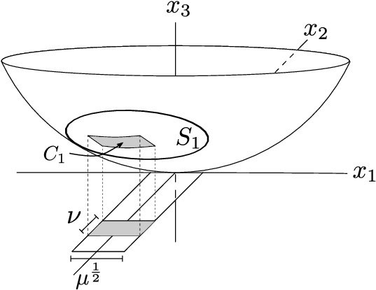
Figure 3: The construction of the cap C1C_{1}.

In higher dimensions we consider as example a modification of the squashed caps in Section 2.7 of [26].

Example 17 (Case n≥3n\geq 3 and μ≤ν≤μ12\mu\leq\nu\leq\mu^{\frac{1}{2}}).

Let Nμ​(S1)N_{\mu}(S_{1}) and Nν​(S2)N_{\nu}(S_{2}) be separated in the paraboloid as in Theorem 7’. Let Lμ⊂ℝn−1L_{\mu}\subset\mathbb{R}^{n-1} be a μ12\mu^{\frac{1}{2}}-neighborhood of the plane {x1=⋯=xn−2=0}\{x_{1}=\cdots=x_{n-2}=0\}. In LμL_{\mu} choose a box C~1\widetilde{C}_{1} of dimensions ν×μ12×⋯×μ12\nu\times\mu^{\frac{1}{2}}\times\cdots\times\mu^{\frac{1}{2}}, so that its lift to the paraboloid lies in S1S_{1}, and thicken it in Nμ​(S1)N_{\mu}(S_{1}) creating so a cap C1C_{1} of dimensions ν×μ12×⋯×μ12×μ\nu\times\mu^{\frac{1}{2}}\times\cdots\times\mu^{\frac{1}{2}}\times\mu; see Figure 3. Now, let C2:=C1+a⊂Nν​(S2)C_{2}:=C_{1}+a\subset N_{\nu}(S_{2}) for some vector aa. After replacing for u^μ=𝟙C1\widehat{u}_{\mu}=\mathds{1}_{C_{1}} and v^ν=𝟙C2\widehat{v}_{\nu}=\mathds{1}_{C_{2}} in the bilinear inequality, we get Kμ,ν​(p′)≥c​μn2​p​ν1pK_{\mu,\nu}(p^{\prime})\geq c\mu^{\frac{n}{2p}}\nu^{\frac{1}{p}}.

The rest of this section is devoted to the proof of the inequality (45) in Theorem 7’. We do first some reductions.

By Galilean and rotational symmetry, we can assume that

S1\displaystyle S_{1} ={(ξ′,12​|ξ′|2)∣|ξ′−c1​e1|≤c2}\displaystyle=\{(\xi^{\prime},\frac{1}{2}\lvert\xi^{\prime}\rvert^{2})\mid\lvert\xi^{\prime}-c_{1}e_{1}\rvert\leq c_{2}\}
S2\displaystyle S_{2} ={(ξ′,12​|ξ′|2)∣|ξ′+c1​e1|≤c2};\displaystyle=\{(\xi^{\prime},\frac{1}{2}\lvert\xi^{\prime}\rvert^{2})\mid\lvert\xi^{\prime}+c_{1}e_{1}\rvert\leq c_{2}\};

the constant CεC_{\varepsilon} in (45) depends on c1c_{1} and c2c_{2}.

It suffices to prove the local inequality

∥fμ​gν∥Lp′​(Bμ−1)≤Cε​μn2​p−ε​ν1p−ε​∥fμ∥2​∥gν∥2.\lVert f_{\mu}g_{\nu}\rVert_{L^{p^{\prime}}(B_{\mu^{-1}})}\leq C_{\varepsilon}\mu^{\frac{n}{2p}-\varepsilon}\nu^{\frac{1}{p}-\varepsilon}\lVert f_{\mu}\rVert_{2}\lVert g_{\nu}\rVert_{2}. (46)

In fact, cover ℝn\mathbb{R}^{n} with balls Bμ−1B_{\mu^{-1}} and choose a bump function ζBμ−1∼1\zeta_{B_{\mu}^{-1}}\sim 1 in Bμ−1B_{\mu^{-1}} so that supp​ζ^Bμ−1⊂Bμ​(0)\text{supp}\,\widehat{\zeta}_{B_{\mu}^{-1}}\subset B_{\mu}(0). Then,

∥fμ​gν∥p′\displaystyle\lVert f_{\mu}g_{\nu}\rVert_{p^{\prime}} ≤∑Bμ−1∥fμ​gν∥Lp′​(Bμ−1)\displaystyle\leq\sum_{B_{\mu^{-1}}}\lVert f_{\mu}g_{\nu}\rVert_{L^{p^{\prime}}(B_{\mu^{-1}})}
≲∑Bμ−1∥(f^μ∗ζ^Bμ−1)∨​(g^ν∗ζ^Bμ−1)∨∥Lp′​(Bμ−1)\displaystyle\lesssim\sum_{B_{\mu^{-1}}}\lVert(\widehat{f}_{\mu}*\widehat{\zeta}_{B_{\mu}^{-1}})^{\vee}(\widehat{g}_{\nu}*\widehat{\zeta}_{B_{\mu}^{-1}})^{\vee}\rVert_{L^{p^{\prime}}(B_{\mu^{-1}})}

The width of the supports of f^μ∗ζ^Bμ−1\widehat{f}_{\mu}*\widehat{\zeta}_{B_{\mu}^{-1}} and g^ν∗ζ^Bμ−1\widehat{g}_{\nu}*\widehat{\zeta}_{B_{\mu}^{-1}} are essentially μ\mu and ν\nu respectively. Hence, we can apply the local bilinear inequality (46) to get

∥fμ​gν∥p′\displaystyle\lVert f_{\mu}g_{\nu}\rVert_{p^{\prime}} ≤Cε​μn2​p−ε​ν1p−ε​∑Bμ−1∥fμ​ζBμ−1∥2​∥gν​ζBμ−1∥2\displaystyle\leq C_{\varepsilon}\mu^{\frac{n}{2p}-\varepsilon}\nu^{\frac{1}{p}-\varepsilon}\sum_{B_{\mu^{-1}}}\lVert f_{\mu}\zeta_{B_{\mu^{-1}}}\rVert_{2}\lVert g_{\nu}\zeta_{B_{\mu^{-1}}}\rVert_{2}
≤Cε​μn2​p−ε​ν1p−ε​(∑Bμ−1∥fμ​ζBμ−1∥22)12​(∑Bμ−1∥gν​ζBμ−1∥22)12\displaystyle\leq C_{\varepsilon}\mu^{\frac{n}{2p}-\varepsilon}\nu^{\frac{1}{p}-\varepsilon}\Big(\sum_{B_{\mu^{-1}}}\lVert f_{\mu}\zeta_{B_{\mu^{-1}}}\rVert_{2}^{2}\Big)^{\frac{1}{2}}\Big(\sum_{B_{\mu^{-1}}}\lVert g_{\nu}\zeta_{B_{\mu^{-1}}}\rVert_{2}^{2}\Big)^{\frac{1}{2}}
≤Cε​μn2​p−ε​ν1p−ε​∥fμ∥2​∥gν∥2,\displaystyle\leq C_{\varepsilon}\mu^{\frac{n}{2p}-\varepsilon}\nu^{\frac{1}{p}-\varepsilon}\lVert f_{\mu}\rVert_{2}\lVert g_{\nu}\rVert_{2},

which is what we wanted to prove.

At scale μ−1\mu^{-1} the function fμf_{\mu} looks like (f​d​S)∨(fdS)^{\vee} for some function ff in the paraboloid, so it suffices to prove the next theorem.

Theorem 18.

Suppose that S1S_{1} and S2S_{2} are two open subsets of the paraboloid in ℝn\mathbb{R}^{n} with diameter ∼1\sim 1 and at distance ∼1\sim 1 of each other. If f​d​SfdS is a measure supported in S1S_{1} and gνg_{\nu} a function with Fourier transform supported in a ν\nu-neighborhood of S2S_{2}, then for 1<R12≤ν−1≤R1<R^{\frac{1}{2}}\leq\nu^{-1}\leq R and for every ε>0\varepsilon>0 it holds

∥(f​d​S)∨​gν∥Lp′​(BR)≤Cε​R12​(1−np)+ε​ν1p−ε​∥f∥L2​(S)​∥gν∥2,\lVert(fdS)^{\vee}g_{\nu}\rVert_{L^{p^{\prime}}(B_{R})}\leq C_{\varepsilon}R^{\frac{1}{2}(1-\frac{n}{p})+\varepsilon}\nu^{\frac{1}{p}-\varepsilon}\lVert f\rVert_{L^{2}(S)}\lVert g_{\nu}\rVert_{2}, (47)

where 1≤p′≤nn−11\leq p^{\prime}\leq\frac{n}{n-1}.

In fact, after a change of variables ξ↦(ξ′,12​|ξ′|2+t)\xi\mapsto(\xi^{\prime},\frac{1}{2}\lvert\xi^{\prime}\rvert^{2}+t) we can write fμf_{\mu} as

fμ​(x)\displaystyle f_{\mu}(x) =∫−μμ(∫f^μ​(ξ′,12​|ξ|2+t)​e​(⟨x′,ξ′⟩+xn​12​|ξ′|2)​𝑑ξ)​e​(xn​t)​𝑑t\displaystyle=\int\limits_{-\mu}^{\mu}\Big(\int\widehat{f}_{\mu}(\xi^{\prime},\frac{1}{2}\lvert\xi\rvert^{2}+t)e(\langle x^{\prime},\xi^{\prime}\rangle+x_{n}\frac{1}{2}\lvert\xi^{\prime}\rvert^{2})\,d\xi\Big)\,e(x_{n}t)\,dt
=∫−μμ(f^μ,t​𝑑S)∨​e​(xn​t)​𝑑t,\displaystyle=\int_{-\mu}^{\mu}(\widehat{f}_{\mu,t}dS)^{\vee}e(x_{n}t)\,dt, (48)

where f^μ,t\widehat{f}_{\mu,t} is a parabolic slice of f^μ\widehat{f}_{\mu}. To bound the local bilinear inequality (46) we use Minkowski to get

∥fμ​gν∥Lp′​(Bμ−1)≤∫−μμ∥(f^μ,t​𝑑S)∨​gν∥Lp′​(Bμ−1)​𝑑t.\lVert f_{\mu}g_{\nu}\rVert_{L^{p^{\prime}}(B_{\mu^{-1}})}\leq\int_{-\mu}^{\mu}\lVert(\widehat{f}_{\mu,t}dS)^{\vee}g_{\nu}\rVert_{L^{p^{\prime}}(B_{\mu^{-1}})}\,dt.

Then, writing μ−1=R\mu^{-1}=R, we can use Theorem 18 and Cauchy-Schwarz inequality to get

∥fμ​gν∥p′\displaystyle\lVert f_{\mu}g_{\nu}\rVert_{p^{\prime}} ≤Cε​μ12​(np−1)−ε​ν1p−ε​∫−μμ∥fμ,t∥2​𝑑t​∥gν∥2\displaystyle\leq C_{\varepsilon}\mu^{\frac{1}{2}(\frac{n}{p}-1)-\varepsilon}\nu^{\frac{1}{p}-\varepsilon}\int_{-\mu}^{\mu}\lVert f_{\mu,t}\rVert_{2}\,dt\;\lVert g_{\nu}\rVert_{2}
≤Cε​μn2​p−ε​ν1p−ε​∥fμ∥2​∥gν∥2.\displaystyle\leq C_{\varepsilon}\mu^{\frac{n}{2p}-\varepsilon}\nu^{\frac{1}{p}-\varepsilon}\lVert f_{\mu}\rVert_{2}\lVert g_{\nu}\rVert_{2}.

Therefore, we must prove now Theorem 18.

The point p′=1p^{\prime}=1 of Theorem 18 can be proven readily. By Cauchy-Schwarz and by the trace inequality ∥(f​d​S)∨∥2≤C​R12​∥f∥L2​(S)\lVert(fdS)^{\vee}\rVert_{2}\leq CR^{\frac{1}{2}}\lVert f\rVert_{L^{2}(S)} we get

∥(f​d​S)∨​gν∥L1​(BR)≤C​R12​∥f∥2​∥gν∥2.\lVert(fdS)^{\vee}g_{\nu}\rVert_{L^{1}(B_{R})}\leq CR^{\frac{1}{2}}\lVert f\rVert_{2}\lVert g_{\nu}\rVert_{2}.

Hence, it suffices to prove the inequality (47) at the point p′=nn−1p^{\prime}=\frac{n}{n-1}.

We begin the proof in the next section with the wave packet decomposition. This decomposition is nowadays a classical change of basis, so we only outline it.

4.1 Wave Packet Decomposition

Let ff be a function in ℝn−1\mathbb{R}^{n-1}, and decompose the space into caps α\alpha of radius R−12R^{-\frac{1}{2}} and center cα∈ℝn−1c_{\alpha}\in\mathbb{R}^{n-1}. Choose a smooth partition of unity {ζα}\{\zeta_{\alpha}\} adapted to the caps α\alpha so that ∑αζα2=1\sum_{\alpha}\zeta_{\alpha}^{2}=1. Use Fourier series adapted to each α\alpha to expand f​ζαf\zeta_{\alpha} into frequencies ω\omega, and develop ff as

f⁡(ξ)=|α|−12​∑α,ωa⁡(α,ω)​ζα​(ξ)​e​(⟨ω,ξ−cα⟩),f(\xi)=\lvert\alpha\rvert^{-\frac{1}{2}}\sum_{\alpha,\omega}a(\alpha,\omega)\zeta_{\alpha}(\xi)e(\langle\omega,\xi-c_{\alpha}\rangle),

where ω=R12​ℤn−1\omega=R^{\frac{1}{2}}\mathbb{Z}^{n-1}. The coefficients aa satisfy the next properties:

a⁡(α,ω)=1|α|12​∫f​ζα​e​(−⟨ω,ξ−cα⟩)​𝑑ξ,\displaystyle a(\alpha,\omega)=\frac{1}{\lvert\alpha\rvert^{\frac{1}{2}}}\int f\zeta_{\alpha}e(-\langle\omega,\xi-c_{\alpha}\rangle)\,d\xi, (49)
∑α,ω|a⁡(α,ω)|2=∥f∥22.\displaystyle\sum_{\alpha,\omega}\lvert a(\alpha,\omega)\rvert^{2}=\lVert f\rVert_{2}^{2}. (50)

By the linearity of the extension operator, we can write (f​d​S)∨(fdS)^{\vee} as

(f​d​S)∨​(x)=∑α,ωa⁡(α,ω)​ϕT⁡(α,ω),(fdS)^{\vee}(x)=\sum_{\alpha,\omega}a(\alpha,\omega)\phi_{T(\alpha,\omega)},

where ϕT\phi_{T} is a function essentially supported in a tube TT of dimensions R12×⋯×R12×RR^{\frac{1}{2}}\times\cdots\times R^{\frac{1}{2}}\times R; the angle and position of TT are determined by α\alpha and ω\omega respectively. Furthermore,

|ϕT​(x)|≤CM​R−n−12​1⟨R−12​(x′+ω+xn​cα)⟩M,for ​|xn|≤R;\lvert\phi_{T}(x)\rvert\leq C_{M}R^{-\frac{n-1}{2}}\frac{1}{\langle R^{-\frac{1}{2}}(x^{\prime}+\omega+x_{n}c_{\alpha})\rangle^{M}},\quad\text{for }\lvert x_{n}\rvert\leq R;

so ϕT\phi_{T} is concentrated in a tube TT of direction (−cα,1)(-c_{\alpha},1) whose main axis passes through (−ω,0)(-\omega,0). We deduce also that for δ>0\delta>0, for x∉Rδ​Tx\notin R^{\delta}T, and for |xn|≤R\lvert x_{n}\rvert\leq R it holds

|ϕT​(x)|≤Cδ​R−100​n,\lvert\phi_{T}(x)\rvert\leq C_{\delta}R^{-100n}, (51)

where possibly Cδ→∞C_{\delta}\to\infty as δ→0\delta\to 0.

The function gνg_{\nu} can be written similarly. We decompose Nν​(S2)N_{\nu}(S_{2}) into rectangles β\beta of dimensions ν×R−12×⋯×R−12\nu\times R^{-\frac{1}{2}}\times\cdots\times R^{-\frac{1}{2}} and center cβ∈ℝnc_{\beta}\in\mathbb{R}^{n}, where cβc_{\beta} is now a point in S2S_{2}. Arguing as before we have

g^ν​(ξ)=|β|−12​∑β,ωb⁡(α,ω)​ζβ​(ξ)​e​(⟨ω,ξ−cβ⟩),\widehat{g}_{\nu}(\xi)=\lvert\beta\rvert^{-\frac{1}{2}}\sum_{\beta,\omega}b(\alpha,\omega)\zeta_{\beta}(\xi)e(\langle\omega,\xi-c_{\beta}\rangle),

where ω\omega belongs to some rotation of the grid ν−1​ℤ×R12​ℤn−1\nu^{-1}\mathbb{Z}\times R^{\frac{1}{2}}\mathbb{Z}^{n-1}. Again, we get

b⁡(β,ω)=1|β|12​∫g^ν​ζβ​e​(−⟨ω,ξ−cβ⟩)​𝑑ξ\displaystyle b(\beta,\omega)=\frac{1}{\lvert\beta\rvert^{\frac{1}{2}}}\int\widehat{g}_{\nu}\zeta_{\beta}e(-\langle\omega,\xi-c_{\beta}\rangle)\,d\xi (52)
∑β,ω|b⁡(β,ω)|2=∥gν∥22.\displaystyle\sum_{\beta,\omega}\lvert b(\beta,\omega)\rvert^{2}=\lVert g_{\nu}\rVert_{2}^{2}. (53)

By the linearity of the Fourier transform, we can write gνg_{\nu} as

gν=∑β,ωb⁡(β,ω)​ϕT⁡(β,ω),g_{\nu}=\sum_{\beta,\omega}b(\beta,\omega)\phi_{T(\beta,\omega)},

where TT are now tubes of dimensions ν−1×R12×⋯×R12\nu^{-1}\times R^{\frac{1}{2}}\times\cdots\times R^{\frac{1}{2}}. Again, we get

|ϕT​(x)|≤CM​ν​R−n−12​1⟨R−12​|x′+ω′+xn​cβ′|+ν​|xn+ωn|⟩M,\displaystyle\lvert\phi_{T}(x)\rvert\leq C_{M}\nu R^{-\frac{n-1}{2}}\frac{1}{\langle R^{-\frac{1}{2}}\lvert x^{\prime}+\omega^{\prime}+x_{n}c_{\beta}^{\prime}\rvert+\nu\lvert x_{n}+\omega_{n}\rvert\rangle^{M}},
|ϕT​(x)|≤Cδ​ν​R−100​n,for ​x∉Rδ​T​ and for ​δ>0.\displaystyle\lvert\phi_{T}(x)\rvert\leq C_{\delta}\nu R^{-100n},\quad\text{for }x\notin R^{\delta}T\text{ and for }\delta>0. (54)

We replace the wave packet decomposition into the bilinear inequality (47), so we must prove that for ∥a∥2=1\lVert a\rVert_{2}=1 and ∥b∥2=1\lVert b\rVert_{2}=1 we have

∥∑T1,T2aT1​bT2​ϕT1​ϕT2∥Lnn−1​(BR)≤Cε​Rε​ν1n−ε.\lVert\sum_{T_{1},T_{2}}a_{T_{1}}b_{T_{2}}\phi_{T_{1}}\phi_{T_{2}}\rVert_{L^{\frac{n}{n-1}}(B_{R})}\leq C_{\varepsilon}R^{\varepsilon}\nu^{\frac{1}{n}-\varepsilon}.

Since |ϕT1|\lvert\phi_{T_{1}}\rvert and |ϕT2|\lvert\phi_{T_{2}}\rvert decay strongly outside the tubes, then we can ignore all the tubes that do not intersect the ball 10​BR10B_{R}, so the number of tubes in each group is ≲RC​n\lesssim R^{Cn}; recall that ν−1≥R12\nu^{-1}\geq R^{\frac{1}{2}}.

Now, for all the terms that satisfy |aT1|\lvert a_{T_{1}}\rvert or |bT2|≲R−Cn\lvert b_{T_{2}}\rvert\lesssim R^{-C_{n}} the contribution to the bilinear inequality is negligible, so we can ignore all these terms and do pigeonholing in |aT1|\lvert a_{T_{1}}\rvert and |bT2|\lvert b_{T_{2}}\rvert; here, we introduce logarithmic losses. Hence, for two collections of tubes 𝕋1\mathbb{T}_{1} and 𝕋2\mathbb{T}_{2} that intersect the ball 10​BR10B_{R} we must prove that

∥∑T1∈𝕋1,T2∈𝕋2ϕT1​ϕT2∥Lnn−1​(BR)≤Cε​Rε​ν1n−ε​|𝕋1|12​|𝕋2|12.\lVert\sum_{T_{1}\in\mathbb{T}_{1},T_{2}\in\mathbb{T}_{2}}\phi_{T_{1}}\phi_{T_{2}}\rVert_{L^{\frac{n}{n-1}}(B_{R})}\leq C_{\varepsilon}R^{\varepsilon}\nu^{\frac{1}{n}-\varepsilon}\lvert\mathbb{T}_{1}\rvert^{\frac{1}{2}}\lvert\mathbb{T}_{2}\rvert^{\frac{1}{2}}. (55)

The proof of this inequality begins with an induction on scales in the next section.

4.2 Induction on Scales

We want to control the quantity

Kν​(R):=sup∥f∥2=∥gν∥2=1∥(f​d​S)∨​gν∥Lp′​(BR).K_{\nu}(R):=\sup_{\lVert f\rVert_{2}=\lVert g_{\nu}\rVert_{2}=1}\lVert(fdS)^{\vee}g_{\nu}\rVert_{L^{p^{\prime}}(B_{R})}.

Rough estimates show that Kμ,ν​(R)K_{\mu,\nu}(R) is finite, thus well defined, and we want to prove that Kμ,ν​(R)≤Cε​Rε​ν1n−εK_{\mu,\nu}(R)\leq C_{\varepsilon}R^{\varepsilon}\nu^{\frac{1}{n}-\varepsilon}.

The induction on scales seeks to control Kμ,ν​(R)K_{\mu,\nu}(R) in terms of Kμ,ν​(R1−δ)K_{\mu,\nu}(R^{1-\delta}) for some δ>0\delta>0, which we keep fixed in what follows, so we lower scales and stop at scale ∼ν−1\sim\nu^{-1}, when Tao’s bilinear theorem provides the best possible upper bound, up to ε\varepsilon-losses. From now on, we write R′R^{\prime} for R1−δR^{1-\delta}.

We begin the induction by breaking up the ball BRB_{R} into balls BR′B_{R^{\prime}}. Now, we define a relationship between balls and tubes, so that a tube is related to a ball if the contribution of ϕT\phi_{T} to the bilinear term is large in that ball. We need first decompose BRB_{R} into balls qq of radius R12R^{\frac{1}{2}}, and now we introduce the following group of definitions for a dyadic number μ2\mu_{2}:

𝕋2​(q):={T2∈𝕋2∣Rδ​T2∩q≠∅}\displaystyle\mathbb{T}_{2}(q):=\{T_{2}\in\mathbb{T}_{2}\mid R^{\delta}T_{2}\cap q\neq\emptyset\} (56)
q⁡(μ2):={q⊂BR∣μ2≤|𝕋2​(q)|<2​μ2}\displaystyle q(\mu_{2}):=\{q\subset B_{R}\mid\mu_{2}\leq\lvert\mathbb{T}_{2}(q)\rvert<2\mu_{2}\} (57)
λ⁡(T1,μ2,BR′):=|{q∈q⁡(μ2)∣q⊂BR′​ and ​Rδ​T1∩q≠∅}|.\displaystyle\lambda(T_{1},\mu_{2},B_{R^{\prime}}):=\lvert\{q\in q(\mu_{2})\mid q\subset B_{R^{\prime}}\text{ and }R^{\delta}T_{1}\cap q\neq\emptyset\}\rvert. (58)
Definition 19 (Relation between tubes and balls).

For every number μ2\mu_{2} and every tube T1∈𝕋1T_{1}\in\mathbb{T}_{1} choose a ball BR′∗​(μ2,T1)B_{R^{\prime}}^{*}(\mu_{2},T_{1}), if it exists, that satisfies

λ⁡(T1,μ2,BR′∗)=maxBR′⁡λ⁡(T1,μ2,BR′)>0.\lambda(T_{1},\mu_{2},B^{*}_{R^{\prime}})=\max_{B_{R^{\prime}}}\lambda(T_{1},\mu_{2},B_{R^{\prime}})>0.

We say that a tube T1∈𝕋1T_{1}\in\mathbb{T}_{1} is related to a ball BR′⊂BRB_{R^{\prime}}\subset B_{R}, or T1∼BR′T_{1}\sim B_{R^{\prime}}, if BR′⊂10​BR′∗​(μ2,T1)B_{R^{\prime}}\subset 10B_{R^{\prime}}^{*}(\mu_{2},T_{1}) for some μ2\mu_{2}. The negation of T1∼BR′T_{1}\sim B_{R^{\prime}} is T1≁BR′T_{1}\nsim B_{R^{\prime}}. Symmetrically, we can define a relation between tubes T2∈𝕋2T_{2}\in\mathbb{T}_{2} and balls BR′B_{R^{\prime}}.

Every tube in 𝕋j\mathbb{T}_{j} intersects a number ≲Rδ\lesssim R^{\delta} of balls BR′⊂BRB_{R^{\prime}}\subset B_{R}, but each tube is related only to ≲log⁡R\lesssim\log R balls. This follows from the condition 1≤μ2≲Rn−12+C​δ1\leq\mu_{2}\lesssim R^{\frac{n-1}{2}+C\delta}.

Now, we bound the bilinear term as

∥∑T1∈𝕋1T2∈𝕋2ϕT1​ϕT2∥Lp′​(BR)\displaystyle\lVert\sum_{\begin{subarray}{c}T_{1}\in\mathbb{T}_{1}\\ T_{2}\in\mathbb{T}_{2}\end{subarray}}\phi_{T_{1}}\phi_{T_{2}}\rVert_{L^{p^{\prime}}(B_{R})} ≤∑BR′⊂BR∥∑T1,T2ϕT1​ϕT2∥Lp′​(BR′)\displaystyle\leq\sum_{B_{R^{\prime}}\subset B_{R}}\lVert\sum_{T_{1},T_{2}}\phi_{T_{1}}\phi_{T_{2}}\rVert_{L^{p^{\prime}}(B_{R^{\prime}})}
≤∑BR′⊂BR(∥∑T1∼BR′,T2∼BR′ϕT1​ϕT2∥Lp′​(BR′)+CLOSE\displaystyle\leq\sum_{B_{R^{\prime}}\subset B_{R}}\Big(\lVert\sum_{T_{1}\sim B_{R^{\prime}},T_{2}\sim B_{R^{\prime}}}\phi_{T_{1}}\phi_{T_{2}}\rVert_{L^{p^{\prime}}(B_{R^{\prime}})}+
OPEN+∥∑T1≁BR′,T2ϕT1​ϕT2∥Lp′​(BR′)+∥∑T1∼BR′,T2≁BR′ϕT1​ϕT2∥Lp′​(BR′)).\displaystyle+\lVert\sum_{T_{1}\nsim B_{R^{\prime}},T_{2}}\phi_{T_{1}}\phi_{T_{2}}\rVert_{L^{p^{\prime}}(B_{R^{\prime}})}+\lVert\sum_{T_{1}\sim B_{R^{\prime}},T_{2}\nsim B_{R^{\prime}}}\phi_{T_{1}}\phi_{T_{2}}\rVert_{L^{p^{\prime}}(B_{R^{\prime}})}\Big).
=I+II+III\displaystyle=\text{I}+\text{II}+\text{III} (59)

For the first term I at the right we use the inductive hypothesis, Cauchy-Schwarz, and the bound |{BR′∣Tj∼BR′}|≲log⁡R\lvert\{B_{R^{\prime}}\mid T_{j}\sim B_{R^{\prime}}\}\rvert\lesssim\log R to get

∑BR′⊂BR∥∑T1∼BR′T2∼BR′ϕT1​ϕT2∥Lp′​(BR′)\displaystyle\sum_{B_{R^{\prime}}\subset B_{R}}\lVert\sum_{\begin{subarray}{c}T_{1}\sim B_{R^{\prime}}\\ T_{2}\sim B_{R^{\prime}}\end{subarray}}\phi_{T_{1}}\phi_{T_{2}}\rVert_{L^{p^{\prime}}(B_{R^{\prime}})} ≤K(R′)∑BR′⊂BR|{T1∼BR′}|12|{T2∼BR′}|12\displaystyle\leq K(R^{\prime})\sum_{{}_{B_{R^{\prime}}}\subset B_{R}}\lvert\{T_{1}\sim B_{R^{\prime}}\}\rvert^{\frac{1}{2}}\lvert\{T_{2}\sim B_{R^{\prime}}\}\rvert^{\frac{1}{2}}
≤K(R′)(∑BR′,T1𝟙{T1∼BR′})12(∑BR′,T2𝟙{T2∼BR′})12\displaystyle\leq K(R^{\prime})\Big(\sum_{B_{R^{\prime}},T_{1}}\mathds{1}_{\{T_{1}\sim B_{R^{\prime}}\}}\Big)^{\frac{1}{2}}\Big(\sum_{B_{R^{\prime}},T_{2}}\mathds{1}_{\{T_{2}\sim B_{R^{\prime}}\}}\Big)^{\frac{1}{2}}
≤C⁡(log⁡R)​K​(R′)​|𝕋1|12​|𝕋2|12.\displaystyle\leq C(\log R)K(R^{\prime})\lvert\mathbb{T}_{1}\rvert^{\frac{1}{2}}\lvert\mathbb{T}_{2}\rvert^{\frac{1}{2}}. (60)

We have bounded so the main contribution with an acceptable logarithmic loss.

We turn now to II in (59); the term III can be similarly controlled, so we will not describe it. We bound the Lnn−1L^{\frac{n}{n-1}}-norm by interpolation between the points p′=1p^{\prime}=1 and p′=2p^{\prime}=2. For p′=1p^{\prime}=1 we use Cauchy-Schwarz and the trace inequality to get

∥∑T1≁BR′,T2ϕT1​ϕT2∥L1​(BR′)≲R12​|𝕋1|12​|𝕋2|12;\lVert\sum_{T_{1}\nsim B_{R^{\prime}},T_{2}}\phi_{T_{1}}\phi_{T_{2}}\rVert_{L^{1}(B_{R^{\prime}})}\lesssim R^{\frac{1}{2}}\lvert\mathbb{T}_{1}\rvert^{\frac{1}{2}}\lvert\mathbb{T}_{2}\rvert^{\frac{1}{2}}; (61)

recall that ∑T1≁BR′ϕT1=(f​d​S)∨\sum_{T_{1}\nsim B_{R^{\prime}}}\phi_{T_{1}}=(fdS)^{\vee} for some function ff in SS, and ∑T2ϕT2=gν\sum_{T_{2}}\phi_{T_{2}}=g_{\nu} for some function gνg_{\nu}, so we only applied the trace theorem to (f​d​S)∨(fdS)^{\vee}, and used (50) and (53). We are left with the point p′=2p^{\prime}=2.

If we are to prove (55) by interpolation, we must get the upper bound

∥∑T1≁BR′,T2ϕT1ϕT2∥L2​(BR′)≲δR12​(1−n2)+C​δν12|𝕋1|12|𝕋2|12.\lVert\sum_{T_{1}\nsim B_{R^{\prime}},T_{2}}\phi_{T_{1}}\phi_{T_{2}}\rVert_{L^{2}(B_{R^{\prime}})}\lesssim_{\delta}R^{\frac{1}{2}(1-\frac{n}{2})+C\delta}\nu^{\frac{1}{2}}\lvert\mathbb{T}_{1}\rvert^{\frac{1}{2}}\lvert\mathbb{T}_{2}\rvert^{\frac{1}{2}}.

This inequality is in general false, if we do not put constrains over the tubes. The simple example f=1f=1 and gν=1g_{\nu}=1 in Nν​(S2)N_{\nu}(S_{2}) is enough, and worst examples can be given. Hence, we have to exploit the special structure of the tubes T1≁BR′T_{1}\nsim B_{R^{\prime}}.

We use the decomposition of BRB_{R} into cubes qq of radius R12R^{\frac{1}{2}} and the definition (57) to write the L2L^{2}-norm as

∥∑T1≁BR′,T2ϕT1​ϕT2∥L2​(BR′)2=∑μ2∑q∈q⁡(μ2)∥∑T1≁BR′,T2ϕT1​ϕT2∥L2​(q)2.\lVert\sum_{T_{1}\nsim B_{R^{\prime}},T_{2}}\phi_{T_{1}}\phi_{T_{2}}\rVert_{L^{2}(B_{R^{\prime}})}^{2}=\sum_{\mu_{2}}\sum_{q\in q(\mu_{2})}\lVert\sum_{T_{1}\nsim B_{R^{\prime}},T_{2}}\phi_{T_{1}}\phi_{T_{2}}\rVert_{L^{2}(q)}^{2}.

By pigeonholing, it suffices to control the norm for a fixed μ2\mu_{2}. We introduce now the definitions

λ⁡(T1,μ2):=|{q∈q⁡(μ2)∣Rδ​T1∩q≠∅}|\displaystyle\lambda(T_{1},\mu_{2}):=\lvert\{q\in q(\mu_{2})\mid R^{\delta}T_{1}\cap q\neq\emptyset\}\rvert (62)
𝕋1​[μ2,λ1]:={T1∈𝕋1∣λ1≤λ⁡(T1,μ2)<2​λ1}.\displaystyle\mathbb{T}_{1}[\mu_{2},\lambda_{1}]:=\{T_{1}\in\mathbb{T}_{1}\mid\lambda_{1}\leq\lambda(T_{1},\mu_{2})<2\lambda_{1}\}. (63)

Since 1≤λ1≲R12+C​δ1\leq\lambda_{1}\lesssim R^{\frac{1}{2}+C\delta}, by pigeonholing again it suffices to prove

∑q∈q⁡(μ2)∥∑T1≁BR′,T1∈𝕋1​[μ2,λ1]T2ϕT1ϕT2∥L2​(q)2≲δR1−n2+C​δν|𝕋1||𝕋2|.\sum_{q\in q(\mu_{2})}\lVert\sum_{\begin{subarray}{c}T_{1}\nsim B_{R^{\prime}},T_{1}\in\mathbb{T}_{1}[\mu_{2},\lambda_{1}]\\ T_{2}\end{subarray}}\phi_{T_{1}}\phi_{T_{2}}\rVert_{L^{2}(q)}^{2}\lesssim_{\delta}R^{1-\frac{n}{2}+C\delta}\nu\lvert\mathbb{T}_{1}\rvert\lvert\mathbb{T}_{2}\rvert. (64)

The case λ⁡(T1,μ2)=0\lambda(T_{1},\mu_{2})=0 is handled with (51). In the next section, we use the special nature of the L2L^{2}-norm to decouple the frequencies.

4.3 Decoupling at Scale R12R^{\frac{1}{2}}

We need first a L2L^{2} upper bound of the bilinear operator. Recall that the extension operator is defined as

(f​𝑑S)∨​(x)=∫ℝn−1f⁡(ξ)​e​(⟨x′,ξ′⟩+xn​φ​(ξ′))​d​ξ′,(fdS)^{\vee}(x)=\int_{\mathbb{R}^{n-1}}f(\xi)e(\langle x^{\prime},\xi^{\prime}\rangle+x_{n}\varphi(\xi^{\prime}))\,d\xi^{\prime},

where φ⁡(ξ′)=12​|ξ′|2\varphi(\xi^{\prime})=\frac{1}{2}\lvert\xi^{\prime}\rvert^{2} and ξ=(ξ′,ξn)\xi=(\xi^{\prime},\xi_{n}). For an open subset S1S_{1} of the paraboloid, we denote by π⁡(S1)\pi(S_{1}) its projection to ℝn−1\mathbb{R}^{n-1}.

We need also the Radon transform of a function, and we define it as

R​f​(ξ′,θ):=∫ℝn−1f⁡(ξ′+η)​δ​(⟨η,θ⟩)​𝑑η;Rf(\xi^{\prime},\theta):=\int_{\mathbb{R}^{n-1}}f(\xi^{\prime}+\eta)\delta\big(\langle\eta,\theta\rangle\big)\,d\eta;

the Radon transform R​f​(ξ′,θ)Rf(\xi^{\prime},\theta) is the integral over the hyperplane with normal θ\theta that passes through ξ′\xi^{\prime}.

Lemma 20.

Let S1S_{1} and S2S_{2} be two open subsets of the paraboloid with radius ∼1\sim 1 and at distance ∼1\sim 1 of each other. Suppose that f​d​SfdS and g​d​SgdS are measures with support in S1S_{1} and S2S_{2} respectively. Then, it holds that

∥(f​d​S)∨​(g​d​S)∨∥22≤C​∥f∥1​supξ′∈π⁡(S1)ξ′′∈π⁡(S2)R​|f|​(ξ′,ξ′−ξ′′|ξ′−ξ′′|)​∥g∥1​∥g∥∞\lVert(fdS)^{\vee}(gdS)^{\vee}\rVert_{2}^{2}\leq C\lVert f\rVert_{1}\sup_{\begin{subarray}{c}\xi^{\prime}\in\pi(S_{1})\\ \xi^{\prime\prime}\in\pi(S_{2})\end{subarray}}R\lvert f\rvert\big(\xi^{\prime},\frac{\xi^{\prime}-\xi^{\prime\prime}}{\lvert\xi^{\prime}-\xi^{\prime\prime}\rvert}\big)\lVert g\rVert_{1}\lVert g\rVert_{\infty} (65)
Proof.

We compute the square of the extension operator as

|(f​d​S)∨​(x)|2\displaystyle\lvert(fdS)^{\vee}(x)\rvert^{2} =∫ℝ2​(n−1)f⁡(ξ1′+ξ2′)​f¯​(ξ2′)\displaystyle=\int_{\mathbb{R}^{2(n-1)}}f(\xi_{1}^{\prime}+\xi_{2}^{\prime})\overline{f}\,(\xi_{2}^{\prime})
e⁡(⟨x′,ξ1′⟩+xn​(φ⁡(ξ1′+ξ2′)−φ⁡(ξ2′)))​d​ξ1′​d​ξ2′\displaystyle\hskip 56.9055pte(\langle x^{\prime},\xi_{1}^{\prime}\rangle+x_{n}(\varphi(\xi_{1}^{\prime}+\xi_{2}^{\prime})-\varphi(\xi_{2}^{\prime})))\,d\xi_{1}^{\prime}d\xi_{2}^{\prime}
=∫(∫f⁡(ξ1′+ξ2′)​f¯​(ξ2′)​δ​(φ⁡(ξ1′+ξ2′)−φ⁡(ξ2′)−t)​d​ξ2′)​e​(⟨x,ξ1⟩)​d​ξ1\displaystyle=\int\Big(\int f(\xi_{1}^{\prime}+\xi_{2}^{\prime})\overline{f}\,(\xi_{2}^{\prime})\delta(\varphi(\xi_{1}^{\prime}+\xi_{2}^{\prime})-\varphi(\xi_{2}^{\prime})-t)\,d\xi_{2}^{\prime}\Big)e(\langle x,\xi_{1}\rangle)\,d\xi_{1}
:=Fˇ​(x),\displaystyle:=\widecheck{F}(x),

where FF is the function in parentheses. Thus, we get

∥(f​𝑑S)∨​(g​𝑑S)∨∥22=∫(F∗G)∨​(x)​𝑑x=(F∗G)∨​(0).\lVert(fdS)^{\vee}(gdS)^{\vee}\rVert_{2}^{2}=\int(F*G)^{\vee}(x)\,dx=(F*G)^{\vee}(0).

We develop the convolution and change variables, so that

∥(f​dS)∨​(g​dS)∨∥22=∫f⁡(ξ2′)​g¯​(ξ2′′)∫f¯​(ξ2′+ξ1′)​g​(ξ2′′+ξ1′)​δ​(φ⁡(ξ2′)−φ⁡(ξ1′+ξ2′)+ξ1,n)​δ​(φ⁡(ξ1′+ξ2′′)−φ⁡(ξ2′′)−ξ1,n)​d​ξ1d​ξ2′​d​ξ2′′.\lVert(fdS)^{\vee}(gdS)^{\vee}\rVert_{2}^{2}=\int f(\xi_{2}^{\prime})\overline{g}\,(\xi_{2}^{\prime\prime})\\ \int\overline{f}\,(\xi_{2}^{\prime}+\xi_{1}^{\prime})g(\xi_{2}^{\prime\prime}+\xi_{1}^{\prime})\delta(\varphi(\xi_{2}^{\prime})-\varphi(\xi_{1}^{\prime}+\xi_{2}^{\prime})+\xi_{1,n})\delta(\varphi(\xi_{1}^{\prime}+\xi_{2}^{\prime\prime})-\varphi(\xi_{2}^{\prime\prime})-\xi_{1,n})\,d\xi_{1}\\ \,d\xi_{2}^{\prime}d\xi_{2}^{\prime\prime}.

We can use Fubini to put inside the integral with respect to ξ1,n\xi_{1,n}, so that after the change of variables ξ1,n↦ξ1,n+φ⁡(ξ1′+ξ2′′)−φ⁡(ξ2′′)\xi_{1,n}\mapsto\xi_{1,n}+\varphi(\xi_{1}^{\prime}+\xi_{2}^{\prime\prime})-\varphi(\xi_{2}^{\prime\prime}) we get

I:=∫δ⁡(φ⁡(ξ2′)−φ⁡(ξ1′+ξ2′)+ξ1,n)​δ​(φ⁡(ξ1′+ξ2′′)−φ⁡(ξ2′′)−ξ1,n)​d​ξ1,n=δ⁡(⟨ξ1′,ξ2′−ξ2′′⟩).\begin{split}I&:=\int\delta(\varphi(\xi_{2}^{\prime})-\varphi(\xi_{1}^{\prime}+\xi_{2}^{\prime})+\xi_{1,n})\delta(\varphi(\xi_{1}^{\prime}+\xi_{2}^{\prime\prime})-\varphi(\xi_{2}^{\prime\prime})-\xi_{1,n})\,d\xi_{1,n}\\ &=\delta(\langle\xi_{1}^{\prime},\xi_{2}^{\prime}-\xi_{2}^{\prime\prime}\rangle).\end{split} (66)

Then, the L2L^{2} norm gets into

∥(f​d​S)∨​(g​d​S)∨∥22\displaystyle\lVert(fdS)^{\vee}(gdS)^{\vee}\rVert_{2}^{2} ≤∫|f|​(ξ2′)​|g|​(ξ2′′)​∫|f|​(ξ2′+ξ1′)​|g|​(ξ2′′+ξ1′)​δ​(⟨ξ1′,ξ2′−ξ2′′⟩)​d​ξ1′​d​ξ2′​d​ξ2′′\displaystyle\leq\int\lvert f\rvert(\xi_{2}^{\prime})\lvert g\rvert(\xi_{2}^{\prime\prime})\int\lvert f\rvert(\xi_{2}^{\prime}+\xi_{1}^{\prime})\lvert g\rvert(\xi_{2}^{\prime\prime}+\xi_{1}^{\prime})\delta(\langle\xi_{1}^{\prime},\xi_{2}^{\prime}-\xi_{2}^{\prime\prime}\rangle)\,d\xi_{1}^{\prime}d\xi_{2}^{\prime}d\xi_{2}^{\prime\prime}
≤∥f∥1​∥g∥1​∥g∥∞​supξ2′,ξ2′′∫|f|​(ξ2′+ξ1′)​δ​(⟨ξ1′,ξ2′−ξ2′′⟩)​d​ξ1′.\displaystyle\leq\lVert f\rVert_{1}\lVert g\rVert_{1}\lVert g\rVert_{\infty}\sup_{\xi_{2}^{\prime},\xi_{2}^{\prime\prime}}\int\lvert f\rvert(\xi_{2}^{\prime}+\xi_{1}^{\prime})\delta(\langle\xi_{1}^{\prime},\xi_{2}^{\prime}-\xi_{2}^{\prime\prime}\rangle)\,d\xi_{1}^{\prime}.

Finally, by the identity δ⁡(a​t)=a−1​δ​(t)\delta(at)=a^{-1}\delta(t), and the condition of separation between S1S_{1} and S2S_{2}, we get

∫|f|​(ξ2′+ξ1′)​δ​(⟨ξ1′,ξ2′−ξ2′′⟩)​d​ξ1′≤C​R​|f|​(ξ2′,ξ2′−ξ2′′|ξ2′−ξ2′′|),\int\lvert f\rvert(\xi_{2}^{\prime}+\xi_{1}^{\prime})\delta(\langle\xi_{1}^{\prime},\xi_{2}^{\prime}-\xi_{2}^{\prime\prime}\rangle)\,d\xi_{1}^{\prime}\leq CR\lvert f\rvert\big(\xi_{2}^{\prime},\frac{\xi_{2}^{\prime}-\xi_{2}^{\prime\prime}}{\lvert\xi_{2}^{\prime}-\xi_{2}^{\prime\prime}\rvert}\big),

which concludes the proof. ∎

We use now Lemma 20 to bound each term at the left side of the inequality (64). To simplify, let us define 𝕋1′:={T1≁BR′}∩𝕋1[μ2,λ1]\mathbb{T}_{1}^{\prime}:=\{T_{1}\nsim B_{R^{\prime}}\}\cap\mathbb{T}_{1}[\mu_{2},\lambda_{1}]. By (49) and (52) we can neglect the contribution from tubes such that Rδ​T∩q=∅R^{\delta}T\cap q=\emptyset. We define so the functions

fq​(ξ)\displaystyle f_{q}(\xi) :=|α|−12​∑T1∈𝕋1′​(q)ζα​(ξ)​e​(⟨ω,ξ−cα⟩)\displaystyle:=\lvert\alpha\rvert^{-\frac{1}{2}}\sum_{T_{1}\in\mathbb{T}_{1}^{\prime}(q)}\zeta_{\alpha}(\xi)e(\langle\omega,\xi-c_{\alpha}\rangle)
g^ν,q​(ξ)\displaystyle\widehat{g}_{\nu,q}(\xi) :=|β|−12​∑T2∈𝕋2​(q)ζβ​(ξ)​e​(⟨ω,ξ−cβ⟩).\displaystyle:=\lvert\beta\rvert^{-\frac{1}{2}}\sum_{T_{2}\in\mathbb{T}_{2}(q)}\zeta_{\beta}(\xi)e(\langle\omega,\xi-c_{\beta}\rangle).

We write gν,qg_{\nu,q} as an average over paraboloids as in (48), and by Minkowski and Cauchy-Schwarz we get

∥∑T1∈𝕋1′​(q),T2∈𝕋2​(q)ϕT1​ϕT2∥L2​(q)2\displaystyle\lVert\sum_{T_{1}\in\mathbb{T}_{1}^{\prime}(q),T_{2}\in\mathbb{T}_{2}(q)}\phi_{T_{1}}\phi_{T_{2}}\rVert_{L^{2}(q)}^{2} ≤∥(fq​d​S)∨​gν,q∥22\displaystyle\leq\lVert(f_{q}dS)^{\vee}g_{\nu,q}\rVert_{2}^{2}
≤∥(fq​𝑑S)∨​∫(g^ν,qt​𝑑S)∨​e​(xn​t)​𝑑t∥22\displaystyle\leq\lVert(f_{q}dS)^{\vee}\int(\widehat{g}_{\nu,q}^{t}dS)^{\vee}e(x_{n}t)\,dt\rVert_{2}^{2}
≤ν​∫∥(fq​𝑑S)∨​(g^ν,qt​𝑑S)∨∥22​𝑑t\displaystyle\leq\nu\int\lVert(f_{q}dS)^{\vee}(\widehat{g}_{\nu,q}^{t}dS)^{\vee}\rVert_{2}^{2}\,dt

We apply Lemma 20 to the integrand, using the inequalities

∥fq∥1≤R−n−14​|𝕋1′​(q)|\displaystyle\lVert f_{q}\rVert_{1}\leq R^{-\frac{n-1}{4}}\lvert\mathbb{T}^{\prime}_{1}(q)\rvert
∥g^ν,qt∥1≤ν−12​R−n−14​|𝕋2​(q)|,∥g^ν,qt∥∞≤ν−12​Rn−14+C​δ,\displaystyle\lVert\widehat{g}_{\nu,q}^{t}\rVert_{1}\leq\nu^{-\frac{1}{2}}R^{-\frac{n-1}{4}}\lvert\mathbb{T}_{2}(q)\rvert,\qquad\lVert\widehat{g}_{\nu,q}^{t}\rVert_{\infty}\leq\nu^{-\frac{1}{2}}R^{\frac{n-1}{4}+C\delta},

to get

∥∑T1∈𝕋1′​(q)T2∈𝕋2​(q)ϕT1​ϕT2∥L2​(q)2≤C​ν​R−n−14+C​δ​|𝕋1′​(q)|​|𝕋2​(q)|​supξ′∈π⁡(S1)ξ′′∈π⁡(S2)R​|fq|​(ξ′,ξ′−ξ′′|ξ′−ξ′′|).\lVert\sum_{\begin{subarray}{c}T_{1}\in\mathbb{T}_{1}^{\prime}(q)\\ T_{2}\in\mathbb{T}_{2}(q)\end{subarray}}\phi_{T_{1}}\phi_{T_{2}}\rVert_{L^{2}(q)}^{2}\leq C\nu R^{-\frac{n-1}{4}+C\delta}\lvert\mathbb{T}^{\prime}_{1}(q)\rvert\lvert\mathbb{T}_{2}(q)\rvert\sup_{\begin{subarray}{c}\xi^{\prime}\in\pi(S_{1})\\ \xi^{\prime\prime}\in\pi(S_{2})\end{subarray}}R\lvert f_{q}\rvert\big(\xi^{\prime},\frac{\xi^{\prime}-\xi^{\prime\prime}}{\lvert\xi^{\prime}-\xi^{\prime\prime}\rvert}\big). (67)

Let 𝕋1′​(q)​(ξ′,ξ′−ξ′′)\mathbb{T}_{1}^{\prime}(q)(\xi^{\prime},\xi^{\prime}-\xi^{\prime\prime}) denote the collection of tubes in 𝕋1′​(q)\mathbb{T}_{1}^{\prime}(q) such that the corresponding cap α\alpha intersects the hyperplane with normal (ξ′−ξ′′)/|ξ′−ξ′′|(\xi^{\prime}-\xi^{\prime\prime})/\lvert\xi^{\prime}-\xi^{\prime\prime}\rvert that passes through ξ′\xi^{\prime}. Then,

supξ′∈π⁡(S1)ξ′′∈π⁡(S2)R​|fq|​(ξ′,ξ′−ξ′′|ξ′−ξ′′|)\displaystyle\sup_{\begin{subarray}{c}\xi^{\prime}\in\pi(S_{1})\\ \xi^{\prime\prime}\in\pi(S_{2})\end{subarray}}R\lvert f_{q}\rvert\big(\xi^{\prime},\frac{\xi^{\prime}-\xi^{\prime\prime}}{\lvert\xi^{\prime}-\xi^{\prime\prime}\rvert}\big) ≤R−n−14+12​supξ′∈π⁡(S1)ξ′′∈π⁡(S2)|𝕋1′​(q)​(ξ′,ξ′−ξ′′)|\displaystyle\leq R^{-\frac{n-1}{4}+\frac{1}{2}}\sup_{\begin{subarray}{c}\xi^{\prime}\in\pi(S_{1})\\ \xi^{\prime\prime}\in\pi(S_{2})\end{subarray}}\lvert\mathbb{T}_{1}^{\prime}(q)(\xi^{\prime},\xi^{\prime}-\xi^{\prime\prime})\rvert
:=R−n−14+12​ν​(q,μ2,λ1);\displaystyle:=R^{-\frac{n-1}{4}+\frac{1}{2}}\nu(q,\mu_{2},\lambda_{1});

we choose the last definition with the same notation as Tao in [25]. We replace in (67) to find

∥∑T1∈𝕋1′​(q),T2∈𝕋2​(q)ϕT1​ϕT2∥L2​(q)2≤C​ν​R1−n2+C​δ​ν​(q,μ2,λ1)​|𝕋1′​(q)|​|𝕋2​(q)|,\lVert\sum_{T_{1}\in\mathbb{T}_{1}^{\prime}(q),T_{2}\in\mathbb{T}_{2}(q)}\phi_{T_{1}}\phi_{T_{2}}\rVert_{L^{2}(q)}^{2}\leq C\nu R^{1-\frac{n}{2}+C\delta}\nu(q,\mu_{2},\lambda_{1})\lvert\mathbb{T}^{\prime}_{1}(q)\rvert\lvert\mathbb{T}_{2}(q)\rvert,

where 𝕋1′:={T1≁BR′}∩𝕋1[μ2,λ1]\mathbb{T}_{1}^{\prime}:=\{T_{1}\nsim B_{R^{\prime}}\}\cap\mathbb{T}_{1}[\mu_{2},\lambda_{1}]. Summing over all the cubes q∈q⁡(μ2)q\in q(\mu_{2}) we get

∑q∈q⁡(μ2)∥∑T1∈𝕋1′​(q),T2∈𝕋2​(q)ϕT1​ϕT2∥L2​(q)2≤C​ν​R1−n2+C​δ​∑q∈q⁡(μ2)ν⁡(q,μ2,λ1)​|𝕋1′​(q)|​|𝕋2​(q)|.\sum_{q\in q(\mu_{2})}\lVert\sum_{T_{1}\in\mathbb{T}_{1}^{\prime}(q),T_{2}\in\mathbb{T}_{2}(q)}\phi_{T_{1}}\phi_{T_{2}}\rVert_{L^{2}(q)}^{2}\leq C\nu R^{1-\frac{n}{2}+C\delta}\sum_{q\in q(\mu_{2})}\nu(q,\mu_{2},\lambda_{1})\lvert\mathbb{T}^{\prime}_{1}(q)\rvert\lvert\mathbb{T}_{2}(q)\rvert. (68)

The term at the right does not involve oscillations, so we achieved a decoupling of the oscillating tubes at the left. To conclude the proof of (64), we must get an upper bound of ν⁡(q,μ2,λ1)\nu(q,\mu_{2},\lambda_{1}), which we do in the next section.

4.4 A Kakeya-type Estimate

In this section we aim to prove the inequality

ν⁡(q0,μ2,λ1)≲RC​δ​|𝕋2|μ2​λ1,\nu(q_{0},\mu_{2},\lambda_{1})\lesssim R^{C\delta}\frac{\lvert\mathbb{T}_{2}\rvert}{\mu_{2}\lambda_{1}}, (69)

for some fixed q0∈q⁡(μ2)q_{0}\in q(\mu_{2}), μ2\mu_{2} and λ1\lambda_{1}. For any ξ′∈π⁡(S1)\xi^{\prime}\in\pi(S_{1}) and ξ′′∈π⁡(S2)\xi^{\prime\prime}\in\pi(S_{2}) we consider then the following bilinear expression

B:=∫q∈q⁡(μ2)BR\10​BR′∑T1∈𝕋1′​(q0)​(ξ′,ξ′−ξ′′)𝟙2​Rδ​T1​∑T2∈𝕋2𝟙2​Rδ​T2.B:=\int\limits_{\begin{subarray}{c}q\in q(\mu_{2})\\ B_{R}\backslash 10B_{R^{\prime}}\end{subarray}}\sum_{T_{1}\in\mathbb{T}^{\prime}_{1}(q_{0})(\xi^{\prime},\xi^{\prime}-\xi^{\prime\prime})}\mathds{1}_{2R^{\delta}T_{1}}\sum_{T_{2}\in\mathbb{T}_{2}}\mathds{1}_{2R^{\delta}T_{2}}.

By the definition of q⁡(μ2)q(\mu_{2}) we get

B≳μ2​∑T1∈𝕋1′​(q0)​(ξ′,ξ′−ξ′′)∫q∈q⁡(μ2)BR\10​BR′𝟙2​Rδ​T1.B\gtrsim\mu_{2}\sum_{T_{1}\in\mathbb{T}^{\prime}_{1}(q_{0})(\xi^{\prime},\xi^{\prime}-\xi^{\prime\prime})}\int_{\begin{subarray}{c}q\in q(\mu_{2})\\ B_{R}\backslash 10B_{R^{\prime}}\end{subarray}}\mathds{1}_{2R^{\delta}T_{1}}.

Since for T1∈{T1≁BR′}∩𝕋1[μ2,λ1]T_{1}\in\{T_{1}\nsim B_{R^{\prime}}\}\cap\mathbb{T}_{1}[\mu_{2},\lambda_{1}] it holds that |{q∈q⁡(μ2)∣Rδ​T1∩q≠∅}|∼λ1\lvert\{q\in q(\mu_{2})\mid R^{\delta}T_{1}\cap q\neq\emptyset\}\rvert\sim\lambda_{1}, we see that

|{q∈q⁡(μ2)∣q⊂BR\10​BR′​ and ​Rδ​T1∩q≠∅}|≳R−δ​λ1.\lvert\{q\in q(\mu_{2})\mid q\subset B_{R}\backslash 10B_{R^{\prime}}\text{ and }R^{\delta}T_{1}\cap q\neq\emptyset\}\rvert\gtrsim R^{-\delta}\lambda_{1}.

Then,

B≳Rn2−C​δ​λ1​μ2​|𝕋1′​(q0)​(ξ′,ξ′−ξ′′)|B\gtrsim R^{\frac{n}{2}-C\delta}\lambda_{1}\mu_{2}\lvert\mathbb{T}^{\prime}_{1}(q_{0})(\xi^{\prime},\xi^{\prime}-\xi^{\prime\prime})\rvert (70)

To get an upper bound of BB, we re-order the summations so that

B≤∑T2∈𝕋2∫BR\10​BR′𝟙2​Rδ​T2​∑T1∈𝕋1′​(q0)​(ξ′,ξ′−ξ′′)𝟙2​Rδ​T1.B\leq\sum_{T_{2}\in\mathbb{T}_{2}}\int_{B_{R}\backslash 10B_{R^{\prime}}}\mathds{1}_{2R^{\delta}T_{2}}\sum_{T_{1}\in\mathbb{T}^{\prime}_{1}(q_{0})(\xi^{\prime},\xi^{\prime}-\xi^{\prime\prime})}\mathds{1}_{2R^{\delta}T_{1}}.

Since all the tubes intersect q0⊂BR′q_{0}\subset B_{R^{\prime}}, we see that

∑T1∈𝕋1′​(q0)​(ξ′,ξ′−ξ′′)𝟙2​Rδ​T1​(x)≲RC​δfor ​x∈BR\10​BR′.\sum_{T_{1}\in\mathbb{T}^{\prime}_{1}(q_{0})(\xi^{\prime},\xi^{\prime}-\xi^{\prime\prime})}\mathds{1}_{2R^{\delta}T_{1}}(x)\lesssim R^{C\delta}\quad\text{for }x\in B_{R}\backslash 10B_{R^{\prime}}.

The tubes in 𝕋1′​(q0)​(ξ′,ξ′−ξ′′)\mathbb{T}^{\prime}_{1}(q_{0})(\xi^{\prime},\xi^{\prime}-\xi^{\prime\prime}) have directions (−cα,1)(-c_{\alpha},1), where cαc_{\alpha} lies at distance <R−12<R^{-\frac{1}{2}} from a hyperplane with normal direction ξ′−ξ′′\xi^{\prime}-\xi^{\prime\prime} that passes through ξ′\xi^{\prime}. Then, the main axis of all the tubes in 𝕋1′​(q0)​(ξ′,ξ′−ξ′′)\mathbb{T}^{\prime}_{1}(q_{0})(\xi^{\prime},\xi^{\prime}-\xi^{\prime\prime}) make an angle <R−12<R^{-\frac{1}{2}} with a hyperplane with normal direction (ξ′−ξ′′,⟨ξ′,ξ′−ξ′′⟩)(\xi^{\prime}-\xi^{\prime\prime},\langle\xi^{\prime},\xi^{\prime}-\xi^{\prime\prime}\rangle) that passes through q0q_{0}. It amounts to saying that the support of ∑T1∈𝕋1′​(q0)​(ξ′,ξ′−ξ′′)𝟙2​Rδ​T1\sum_{T_{1}\in\mathbb{T}^{\prime}_{1}(q_{0})(\xi^{\prime},\xi^{\prime}-\xi^{\prime\prime})}\mathds{1}_{2R^{\delta}T_{1}} lies inside the R12+δR^{\frac{1}{2}+\delta}-neighborhood of a hyperplane that passes through q0q_{0}. Furthermore, every tube from 𝕋2\mathbb{T}_{2} intersects the hyperplane transversally, making an angle >c>c uniformly. Then,

B≲Rn2+C​δ​|𝕋2|.B\lesssim R^{\frac{n}{2}+C\delta}\lvert\mathbb{T}_{2}\rvert. (71)

We use (70) and (71) to conclude that

|𝕋1′​(q0)​(ξ′,ξ′−ξ′′)|≲RC​δ​|𝕋2|λ1​μ2,\lvert\mathbb{T}^{\prime}_{1}(q_{0})(\xi^{\prime},\xi^{\prime}-\xi^{\prime\prime})\rvert\lesssim R^{C\delta}\frac{\lvert\mathbb{T}_{2}\rvert}{\lambda_{1}\mu_{2}},

which is what we wanted to prove.

4.5 End of the Proof

In this section we reap all the bounds we have obtained. We plug (69) into (68) to get

∑q∈q⁡(μ2)∥∑T1∈𝕋1′​(q)T2∈𝕋2​(q)ϕT1​ϕT2∥L2​(q)2\displaystyle\sum_{q\in q(\mu_{2})}\lVert\sum_{\begin{subarray}{c}T_{1}\in\mathbb{T}_{1}^{\prime}(q)\\ T_{2}\in\mathbb{T}_{2}(q)\end{subarray}}\phi_{T_{1}}\phi_{T_{2}}\rVert_{L^{2}(q)}^{2} ≤ν​R1−n2+C​δ​|𝕋2|​∑q∈q⁡(μ2)λ1−1​|𝕋1​[μ2,λ1]​(q)|\displaystyle\leq\nu R^{1-\frac{n}{2}+C\delta}\lvert\mathbb{T}_{2}\rvert\sum_{q\in q(\mu_{2})}\lambda_{1}^{-1}\lvert\mathbb{T}_{1}[\mu_{2},\lambda_{1}](q)\rvert
≲νR1−n2+C​δ|𝕋2|∑T1∈𝕋1​[λ1,μ2]λ1−1∑q∈q⁡(μ2)𝟙{T1∩Rδq≠∅}\displaystyle\lesssim\nu R^{1-\frac{n}{2}+C\delta}\lvert\mathbb{T}_{2}\rvert\sum_{T_{1}\in\mathbb{T}_{1}[\lambda_{1},\mu_{2}]}\lambda_{1}^{-1}\sum_{\begin{subarray}{c}q\in q(\mu_{2})\\ \end{subarray}}\mathds{1}_{\{T_{1}\cap R^{\delta}q\neq\emptyset\}}
≲ν​R1−n2+C​δ​|𝕋1|​|𝕋2|,\displaystyle\lesssim\nu R^{1-\frac{n}{2}+C\delta}\lvert\mathbb{T}_{1}\rvert\lvert\mathbb{T}_{2}\rvert,

This concludes the proof of (64).

We interpolate the bilinear norm between the points p′=1p^{\prime}=1 in (61) and p′=2p^{\prime}=2 in (64) to get

∥∑T1≁BR′,T2ϕT1​ϕT2∥Lnn−1​(BR′)≤Cδ​(log⁡R)C​RC​δ​ν1n​|𝕋1|12​|𝕋2|12.\lVert\sum_{T_{1}\nsim B_{R^{\prime}},T_{2}}\phi_{T_{1}}\phi_{T_{2}}\rVert_{L^{\frac{n}{n-1}}(B_{R^{\prime}})}\leq C_{\delta}(\log R)^{C}R^{C\delta}\nu^{\frac{1}{n}}\lvert\mathbb{T}_{1}\rvert^{\frac{1}{2}}\lvert\mathbb{T}_{2}\rvert^{\frac{1}{2}}.

This bound joins the inequalities (59) and (60) to yield

∥∑T1∈𝕋1T2∈𝕋2ϕT1​ϕT2∥Lnn−1​(BR)≤Cδ​(log⁡R)C​(Kν​(R′)+RC​δ​ν1n)​|𝕋1|12​|𝕋2|12;\lVert\sum_{\begin{subarray}{c}T_{1}\in\mathbb{T}_{1}\\ T_{2}\in\mathbb{T}_{2}\end{subarray}}\phi_{T_{1}}\phi_{T_{2}}\rVert_{L^{\frac{n}{n-1}}(B_{R})}\leq C_{\delta}(\log R)^{C}(K_{\nu}(R^{\prime})+R^{C\delta}\nu^{\frac{1}{n}})\lvert\mathbb{T}_{1}\rvert^{\frac{1}{2}}\lvert\mathbb{T}_{2}\rvert^{\frac{1}{2}};

in other words,

Kν​(R)≤Cδ​(log⁡R)C​(Kν​(R1−δ)+RC​δ​ν1n).K_{\nu}(R)\leq C_{\delta}(\log R)^{C}(K_{\nu}(R^{1-\delta})+R^{C\delta}\nu^{\frac{1}{n}}).

When we iterate, we get at the NN-th step

Kν​(R)≤CδN​(log⁡R)N​C​(Kν​(R(1−δ)N)+N​RC​δ​ν1n).K_{\nu}(R)\leq C_{\delta}^{N}(\log R)^{NC}(K_{\nu}(R^{(1-\delta)^{N}})+NR^{C\delta}\nu^{\frac{1}{n}}).

We stop when R(1−δ)N≤ν−1<R(1−δ)N−1R^{(1-\delta)^{N}}\leq\nu^{-1}<R^{(1-\delta)^{N-1}}; the number of steps is

N≤−1log⁡(1−δ)+1≤2​δ−1.N\leq-\frac{1}{\log(1-\delta)}+1\leq 2\delta^{-1}.

If r≤ν−1r\leq\nu^{-1}, then we can average over translations of the paraboloid and apply Tao’s bilinear to get Kν​(r)≤Cε​r1−n+22​p+ε​ν12K_{\nu}(r)\leq C_{\varepsilon}r^{1-\frac{n+2}{2p}+\varepsilon}\nu^{\frac{1}{2}}. We have thus that

Kν​(R)≤Cδ​RC​δ​(ν−1+n+22​n+12+ν1n)≤Cδ​RC​δ​ν1n.K_{\nu}(R)\leq C_{\delta}R^{C\delta}(\nu^{-1+\frac{n+2}{2n}+\frac{1}{2}}+\nu^{\frac{1}{n}})\leq C_{\delta}R^{C\delta}\nu^{\frac{1}{n}}.

This concludes the proof of Theorem 18, which implies Theorem 7’.

4.5.1 Additional Remarks

We indicate here the changes we need to do for surfaces of elliptic type or the hemisphere. The argument is sufficiently robust to admit perturbations.

For surfaces of ε\varepsilon-elliptic type, the semi-norms ∥∂NΦ∥∞\lVert\partial^{N}\Phi\rVert_{\infty} enter in the constants CδC_{\delta} of (51) and (54). Since the eigenvalues of D2​ΦD^{2}\Phi are close to one, then the tubes have approximately the same length.

The delta function in (66) gets into

δ⁡(Φ⁡(ξ2′)−Φ⁡(ξ1′+ξ2′)+Φ⁡(ξ1′+ξ2′′)−Φ⁡(ξ2′′))=δ⁡(⟨A⁡(ξ2′−ξ2′′),ξ1′⟩)\delta(\Phi(\xi_{2}^{\prime})-\Phi(\xi_{1}^{\prime}+\xi_{2}^{\prime})+\Phi(\xi_{1}^{\prime}+\xi_{2}^{\prime\prime})-\Phi(\xi_{2}^{\prime\prime}))=\delta(\langle A(\xi_{2}^{\prime}-\xi_{2}^{\prime\prime}),\xi_{1}^{\prime}\rangle)

for some matrix AA with eigenvalues in [1−ε,1+ε][1-\varepsilon,1+\varepsilon]. Then |⟨A⁡(ξ2′−ξ2′′),ξ1′⟩−⟨ξ2′−ξ2′′,ξ1′⟩|≤C​ε\lvert\langle A(\xi_{2}^{\prime}-\xi_{2}^{\prime\prime}),\xi_{1}^{\prime}\rangle-\langle\xi_{2}^{\prime}-\xi_{2}^{\prime\prime},\xi_{1}^{\prime}\rangle\rvert\leq C\varepsilon, and instead of an integral over the hyperplane HH with normal direction ξ2′−ξ2′′\xi_{2}^{\prime}-\xi_{2}^{\prime\prime} that passes through ξ2′\xi_{2}^{\prime}, we integrate over a (n−2)(n-2)-surface H~\tilde{H} that lies in a ε\varepsilon-neighborhood of HH and passes through ξ2′\xi_{2}^{\prime}.

A tube associated with a cap with center cαc_{\alpha} has velocity (−∇Φ​(cα),1)(-\nabla\Phi(c_{\alpha}),1). If P~⊂ℝn\tilde{P}\subset\mathbb{R}^{n} is a (n−1)(n-1)-cone with center in a cube qq generated by all the lines with directions (−∇Φ​(η),1)(-\nabla\Phi(\eta),1) for η∈H~\eta\in\tilde{H}, then we must verify that all the tubes coming from the separated set S2S_{2} are transversal to P~\tilde{P}. In fact, notice that for any point ξ2′+ξ1′∈H~\xi_{2}^{\prime}+\xi_{1}^{\prime}\in\tilde{H}, a vector vv tangent to H~\tilde{H} satisfies the equation

⟨∇Φ​(ξ1′+ξ2′′)−∇Φ​(ξ1′+ξ2′),v⟩=0;\langle\nabla\Phi(\xi_{1}^{\prime}+\xi_{2}^{\prime\prime})-\nabla\Phi(\xi_{1}^{\prime}+\xi_{2}^{\prime}),v\rangle=0;

hence, ⟨A⁡(ξ2′′−ξ2′),v⟩=0\langle A(\xi_{2}^{\prime\prime}-\xi_{2}^{\prime}),v\rangle=0 for some matrix AA close to II. Then, the vectors normal to P~\tilde{P} have the form (A⁡(ξ2′′−ξ2′),⟨∇Φ​(ξ2′+ξ1′),A⁡(ξ2′′−ξ2′)⟩)(A(\xi_{2}^{\prime\prime}-\xi_{2}^{\prime}),\langle\nabla\Phi(\xi_{2}^{\prime}+\xi_{1}^{\prime}),A(\xi_{2}^{\prime\prime}-\xi_{2}^{\prime})\rangle). If we take the inner product of these vectors with (−∇Φ​(η2),1)(-\nabla\Phi(\eta_{2}),1) for η2∈π⁡(S2)\eta_{2}\in\pi(S_{2}), then we get

⟨A⁡(ξ2′′−ξ2′),∇Φ​(ξ2′+ξ1′)−∇Φ​(η2)⟩=⟨A⁡(ξ2′′−ξ2′),A′​(ξ2′+ξ1′−η2)⟩;\langle A(\xi_{2}^{\prime\prime}-\xi_{2}^{\prime}),\nabla\Phi(\xi_{2}^{\prime}+\xi_{1}^{\prime})-\nabla\Phi(\eta_{2})\rangle=\langle A(\xi_{2}^{\prime\prime}-\xi_{2}^{\prime}),A^{\prime}(\xi_{2}^{\prime}+\xi_{1}^{\prime}-\eta_{2})\rangle;

hence, the inner product is basically equal to ⟨η1−η2,η1′−η2′⟩\langle\eta_{1}-\eta_{2},\eta_{1}^{\prime}-\eta_{2}^{\prime}\rangle for all the pairs η1,η1′∈π⁡(S1)\eta_{1},\eta_{1}^{\prime}\in\pi(S_{1}) and η2,η2′∈π⁡(S2)\eta_{2},\eta_{2}^{\prime}\in\pi(S_{2}), and |⟨η1−η2,η1′−η2′⟩|≥c>0\lvert\langle\eta_{1}-\eta_{2},\eta_{1}^{\prime}-\eta_{2}^{\prime}\rangle\rvert\geq c>0, then P~\tilde{P} is uniformly transversal to all the tubes coming from S2S_{2}. The estimates hold uniformly in ε≪1\varepsilon\ll 1.

The case of the hemi-sphere is similar. The term (66) is almost as simple as for the paraboloid. By symmetry, we can assume that ξ2′=−a​e1\xi_{2}^{\prime}=-ae_{1} and ξ2′′=a​e1\xi_{2}^{\prime\prime}=ae_{1} for some 0<a≤12+1100<a\leq\frac{1}{\sqrt{2}}+\frac{1}{10}. Then, the (n−2)(n-2)-surface H~\tilde{H} is again a hyperplane HH with normal direction e1e_{1} that passes through ξ2′\xi_{2}^{\prime}. The cone P~\tilde{P} is a translation of a portion of the quadratic cone {ξ∣ξ12=a2​|ξ|2}\{\xi\mid\xi_{1}^{2}=a^{2}\lvert\xi\rvert^{2}\}. It is intuitively clear that the portion of the cone generated by direction from S1S_{1} is uniformly transversal to tubes from S2S_{2}.

Notations

  • •

    Relations: A≲ϵBA\lesssim_{\epsilon}B if A≤Cϵ​BA\leq C_{\epsilon}B; A∼BA\sim B if A≲B≲AA\lesssim B\lesssim A; A≪1A\ll 1 if A≤cA\leq c, where cc is chosen sufficiently small.

  • •

    Various: e⁡(z):=e2​π​i​ze(z):=e^{2\pi iz}, ⟨x⟩=(1+|x|2)12\langle x\rangle=(1+\lvert x\rvert^{2})^{\frac{1}{2}}, Br​(x)B_{r}(x) a ball of radius rr with center at xx. −∫Mdτ:=1M∫M2​Mdτ\mathchoice{{\vbox{\hbox{$\textstyle-$ }}\kern-7.83337pt}}{{\vbox{\hbox{$\scriptstyle-$ }}\kern-6.11674pt}}{{\vbox{\hbox{$\scriptscriptstyle-$ }}\kern-5.48965pt}}{{\vbox{\hbox{$\scriptscriptstyle-$ }}\kern-5.31259pt}}\!\int_{M}\,d\tau:=\frac{1}{M}\int_{M}^{2M}\,d\tau. a+:=a+εa+:=a+\varepsilon for ε≪1\varepsilon\ll 1. |E|\lvert E\rvert is the Lebesgue measure of a set E⊂ℝnE\subset\mathbb{R}^{n}, or the cardinality of a finite set EE. If TT is a tube with main axis ll, then A​TAT is a dilation of TT by a factor A>0A>0 and same main axis ll.

  • •

    Multipliers: m⁡(D)​f=(m​f^)∨m(D)f=(m\widehat{f})^{\vee}, where mm stands for multiplier; P​f=m⁡(D)​fPf=m(D)f, where mm is a smooth cut-off for a set of frequencies where we want to project to.

  • •

    The operator Δζ:=Δ+ζ⋅∇\Delta_{\zeta}:=\Delta+\zeta\cdot\nabla has symbol pζ(ξ):=−|ξ|2+2iζ⋅∇p_{\zeta}(\xi):=-\lvert\xi\rvert^{2}+2i\zeta\cdot\nabla and characteristic Σζ:={ξ∣pζ​(ξ)=0}\Sigma_{\zeta}:=\{\xi\mid p_{\zeta}(\xi)=0\}.

  • •

    ζ⁡(U,τ):=τ⁡(U​e1−i​U​e2)\zeta(U,\tau):=\tau(Ue_{1}-iUe_{2}), where {ei}\{e_{i}\} is the canonical basis, τ≥1\tau\geq 1 and U∈OdU\in O_{d} is a rotation.

  • •

    ∥u∥X˙ζb2:=∫|pζ​(ξ)|2​b​|u^​(ξ)|2​𝑑ξ\lVert u\rVert_{\dot{X}^{b}_{\zeta}}^{2}:=\int\lvert p_{\zeta}(\xi)\rvert^{2b}\lvert\widehat{u}(\xi)\rvert^{2}\,d\xi.

  • •

    ∥u∥Xζ,σb2:=∫(|pζ​(ξ)|+σ)2​b​|u^​(ξ)|2​𝑑ξ\lVert u\rVert_{X^{b}_{\zeta,\sigma}}^{2}:=\int(\lvert p_{\zeta}(\xi)\rvert+\sigma)^{2b}\lvert\widehat{u}(\xi)\rvert^{2}\,d\xi for σ>0\sigma>0; ∥u∥Xζb=∥u∥Xζ,|ζ|b\lVert u\rVert_{X^{b}_{\zeta}}=\lVert u\rVert_{X^{b}_{\zeta,\lvert\zeta\rvert}}.

  • •

    Sobolev-Slobodeckij spaces: For 1≤p<∞1\leq p<\infty, Ws,p​(ℝd)W^{s,p}(\mathbb{R}^{d}) is the space of distributions ff such that

    ∥f∥s,p\displaystyle\lVert f\rVert_{s,p} :=∑|α|≤s∥Dαf∥pfor s integer.\displaystyle:=\sum_{\lvert\alpha\rvert\leq s}\lVert D^{\alpha}f\rVert_{p}\quad\text{for }s\text{ integer.} (72)
    ∥f∥s,p\displaystyle\lVert f\rVert_{s,p} :=∥P≤1​f∥p+(∑k>02s​k​p​∥Pk​f∥pp)1p<∞for ​0<s≠integer.\displaystyle:=\lVert P_{\leq 1}f\rVert_{p}+\Big(\sum_{k>0}2^{skp}\lVert P_{k}f\rVert_{p}^{p}\Big)^{\frac{1}{p}}<\infty\quad\text{for }0<s\neq\text{integer.} (73)

    For a domain Ω⊂ℝd\Omega\subset\mathbb{R}^{d}, we define Ws,p​(Ω):={f|Ω∣f∈Ws,p​(ℝd)}W^{s,p}(\Omega):=\{f|_{\Omega}\mid f\in W^{s,p}(\mathbb{R}^{d})\}. The space W∘s,p​(Ω)\accentset{\circ}{W}^{s,p}(\Omega) is the completion in Ws,p​(ℝd)W^{s,p}(\mathbb{R}^{d}) of test functions D⁡(Ω):={φ∈C∞​(Ω)∣supp​φ⋐Ω}D(\Omega):=\{\varphi\in C^{\infty}(\Omega)\mid\text{supp}\,\varphi\Subset\Omega\}. For further details, see e.g. [28, 19].

  • •

    (f​𝑑S)∨​(x):=∫ℝn−1f⁡(ξ)​e​(⟨x′,ξ⟩+xn​φ​(ξ))​𝑑ξ(fdS)^{\vee}(x):=\int_{\mathbb{R}^{n-1}}f(\xi)e(\langle x^{\prime},\xi\rangle+x_{n}\varphi(\xi))\,d\xi, where SS is the graph of φ\varphi and (x′,xn)∈ℝn(x^{\prime},x_{n})\in\mathbb{R}^{n}.

References

  • [1] K. Astala and L. Päivärinta. Calderón’s inverse conductivity problem in the plane. Ann. of Math. (2), 163(1):265–299, 2006.
  • [2] J. Bourgain. Refinements of Strichartz’ inequality and applications to 22D-NLS with critical nonlinearity. Internat. Math. Res. Notices, (5):253–283, 1998.
  • [3] J. Bourgain, C. Demeter, and L. Guth. Proof of the main conjecture in Vinogradov’s mean value theorem for degrees higher than three. Ann. of Math. (2), 184(2):633–682, 2016.
  • [4] R. Brown. Global uniqueness in the impedance-imaging problem for less regular conductivities. SIAM J. Math. Anal., 27(4):1049–1056, 1996.
  • [5] R. Brown. Recovering the conductivity at the boundary from the Dirichlet to Neumann map: a pointwise result. J. Inverse Ill-Posed Probl., 9(6):567–574, 2001.
  • [6] R. Brown and R. Torres. Uniqueness in the inverse conductivity problem for conductivities with 3/23/2 derivatives in Lp,p>2​nL^{p},\ p>2n. J. Fourier Anal. Appl., 9(6):563–574, 2003.
  • [7] A. Calderón. On an inverse boundary value problem. In Seminar on Numerical Analysis and its Applications to Continuum Physics (Rio de Janeiro, 1980), pages 65–73. Soc. Brasil. Mat., Rio de Janeiro, 1980.
  • [8] P. Caro and K. Rogers. Global uniqueness for the Calderón problem with Lipschitz conductivities. Forum Math. Pi, 4:e2, 28, 2016.
  • [9] D. Dos Santos Ferreira, C. Kenig, M. Salo, and G. Uhlmann. Limiting Carleman weights and anisotropic inverse problems. Invent. Math., 178(1):119–171, 2009.
  • [10] C. Fefferman. A note on spherical summation multipliers. Israel J. Math., 15:44–52, 1973.
  • [11] B. Haberman. Uniqueness in Calderón’s problem for conductivities with unbounded gradient. Comm. Math. Phys., 340(2):639–659, 2015.
  • [12] B. Haberman and D. Tataru. Uniqueness in Calderón’s problem with Lipschitz conductivities. Duke Math. J., 162(3):496–516, 2013.
  • [13] S. Ham, Y. Kwon, and S. Lee. Uniqueness in the calderón problem and bilinear restriction estimates. arXiv:1903.09382v2 [math.AP], 2019.
  • [14] C. Kenig, A. Ruiz, and C. Sogge. Uniform Sobolev inequalities and unique continuation for second order constant coefficient differential operators. Duke Math. J., 55(2):329–347, 1987.
  • [15] C. Kenig, J. Sjöstrand, and G. Uhlmann. The Calderón problem with partial data. Ann. of Math. (2), 165(2):567–591, 2007.
  • [16] R. Kohn and M. Vogelius. Determining conductivity by boundary measurements. Comm. Pure Appl. Math., 37(3):289–298, 1984.
  • [17] S. Lee. Improved bounds for Bochner-Riesz and maximal Bochner-Riesz operators. Duke Math. J., 122(1):205–232, 2004.
  • [18] S. Lee. Bilinear restriction estimates for surfaces with curvatures of different signs. Trans. Amer. Math. Soc., 358(8):3511–3533, 2006.
  • [19] J. Marschall. The trace of Sobolev-Slobodeckij spaces on Lipschitz domains. Manuscripta Math., 58(1-2):47–65, 1987.
  • [20] P. Mattila. Fourier analysis and Hausdorff dimension, volume 150 of Cambridge Studies in Advanced Mathematics. Cambridge University Press, Cambridge, 2015.
  • [21] H. Nguyen and D. Spirn. Recovering a potential from cauchy data via complex geometrical optics solutions. arXiv:1403.2255v2 [math.AP], 2014.
  • [22] A. Seagar, D. Barber, and B. Brown. Electrical impedance imaging. IEE Proceedings, 134(2):201–210, 1987.
  • [23] E. Stein. Harmonic analysis: real-variable methods, orthogonality, and oscillatory integrals, volume 43 of Princeton Mathematical Series. Princeton University Press, Princeton, NJ, 1993. With the assistance of Timothy S. Murphy, Monographs in Harmonic Analysis, III.
  • [24] J. Sylvester and G. Uhlmann. A global uniqueness theorem for an inverse boundary value problem. Ann. of Math. (2), 125(1):153–169, 1987.
  • [25] T. Tao. A sharp bilinear restrictions estimate for paraboloids. Geom. Funct. Anal., 13(6):1359–1384, 2003.
  • [26] T. Tao, A. Vargas, and L. Vega. A bilinear approach to the restriction and Kakeya conjectures. J. Amer. Math. Soc., 11(4):967–1000, 1998.
  • [27] P. Tomas. A restriction theorem for the Fourier transform. Bull. Amer. Math. Soc., 81:477–478, 1975.
  • [28] H. Triebel. Theory of function spaces, volume 78 of Monographs in Mathematics. Birkhäuser Verlag, Basel, 1983.
  • [29] A. Vargas. Restriction theorems for a surface with negative curvature. Math. Z., 249(1):97–111, 2005.
  • [30] T. Wolff. A sharp bilinear cone restriction estimate. Ann. of Math. (2), 153(3):661–698, 2001.