LU TP 19-39

Employing flavor symmetries to understand the apparent arbitrariness of the quark masses and mixings in the Standard Model (SM) is an exercise continuing for decades. The Yukawa Lagrangian of the SM also contains many redundant parameters, which is not a very attractive feature of the model. Therefore, theoretical constructions beyond the SM (BSM) that attempt to address these issues in a minimalistic manner should deserve some attention. To this end, we notice that the quark masses and mixings adhere to the following approximate pattern,

$\displaystyle m_{u}\approx 0\,,\quad m_{d}\approx 0\,,\quad V_{\rm CKM}=\begin{pmatrix}\cos\theta_{C}&\sin\theta_{C}&0\\ -\sin\theta_{C}&\cos\theta_{C}&0\\ 0&0&1\end{pmatrix},$

(1)

where $V_{\rm CKM}$ stands for the Cabibbo–Kobayashi–Maskawa (CKM) matrix with only the Cabibbo block retained. The quantity $\sin\theta_{C}\approx 0.22$ appearing in Eq. (1) denote the Cabibbo mixing parameter. In this approximate scenario, we note that there are only five nonzero parameters in the quark sector, namely, four quark masses ($m_{c}$, $m_{s}$, $m_{t}$, $m_{b}$) and the Cabibbo parameter itself. Thus, a flavor-model that contains five or fewer parameters in its quark Yukawa Lagrangian, might have a better aesthetic appeal than the SM in the sense that many of the redundant parameters have been erased by the flavor symmetry leaving behind only the relevant ones. The model can be even more attractive, if the zeros in Eq. (1) emerge naturally as a consequence of the Yukawa textures imposed by the flavor symmetry. As we will demonstrate, these objectives can be achieved in the simple framework of a two Higgs-doublet model (2HDM)[1, 2] with a $D_{4}$ flavor symmetry.

The discrete symmetry group $D_{4}$ has five irreducible representations: $\mathbf{1}_{++}$, $\mathbf{1}_{+-}$, $\mathbf{1}_{-+}$, $\mathbf{1}_{--}$ and $\mathbf{2}$[3, 4]. We pick a basis such that the generators in the $\mathbf{2}$ representation are given by

$\displaystyle a=\begin{bmatrix}0&-1\\ 1&0\end{bmatrix}\,,\qquad b=\begin{bmatrix}1&0\\ 0&-1\end{bmatrix}\,.$

(2)

Note that $a$ is of order 4, whereas $b$ is of order 2. The rest of the elements can be obtained by taking products of powers of these two elements. In this basis, the relevant tensor products are obtained as

	$\displaystyle\begin{bmatrix}x_{1}\\ x_{2}\end{bmatrix}_{\mathbf{2}}\otimes\begin{bmatrix}y_{1}\\ y_{2}\end{bmatrix}_{\mathbf{2}}$	$\displaystyle=$	$\displaystyle[x_{1}y_{1}+x_{2}y_{2}]_{\mathbf{1}_{++}}\oplus[x_{1}y_{2}-x_{2}y_{1}]_{\mathbf{1}_{--}}$		(3a)
			$\displaystyle\oplus\,[x_{1}y_{2}+x_{2}y_{1}]_{\mathbf{1}_{-+}}\oplus[x_{1}y_{1}-x_{2}y_{2}]_{\mathbf{1}_{+-}}\,,$
	$\displaystyle\mathbf{1}_{rs}\otimes\mathbf{1}_{r^{\prime}s^{\prime}}$	$\displaystyle=$	$\displaystyle\mathbf{1}_{r{{}^{\prime\prime}}s{{}^{\prime\prime}}}\,,$		(3b)

where $r{{}^{\prime\prime}}=r\cdot r^{\prime}$ and $s{{}^{\prime\prime}}=s\cdot s^{\prime}$. The quark fields are assumed to transform under $D_{4}$ in the following way:

	$\displaystyle{\bf 2}\,\,:\,\,\begin{bmatrix}Q_{1}\\ Q_{2}\end{bmatrix},\;\begin{bmatrix}p_{1R}\\ p_{2R}\end{bmatrix},\;\begin{bmatrix}n_{1R}\\ n_{2R}\end{bmatrix}\,,$		(4a)
	$\displaystyle\mathbf{1}_{++}\,\,:\,\,Q_{3}\,,\qquad\mathbf{1}_{--}\,\,:\,\,p_{3R}\,,\qquad\mathbf{1}_{-+}\,\,:\,\,n_{3R}\,,$		(4b)

where the $Q_{A}$’s ($A=1,2,3$) are the usual left-handed $\rm SU(2)$ quark doublets, whereas the $p_{AR}$’s and $n_{AR}$’s are the right-handed up-type and down-type quark fields respectively, which are singlets of the $\rm SU(2)$ part of the gauge symmetry. Note that the square brackets in Eqs. (2), (3) and (4) as well as in the subsequent text, denote the representations of $D_{4}$ and has nothing to do with the representation of the enclosed fields under $\rm SU(2)$. In the Higgs sector there are two $\rm SU(2)$ doublets $\phi_{k}$ ($k=1,2)$ and their transformation under the $D_{4}$ symmetry is as follows:

$\displaystyle\mathbf{2}$

$\displaystyle:$

$\displaystyle\begin{bmatrix}\phi_{1}\\ \phi_{2}\end{bmatrix}\,.$

(5)

The most general Yukawa Lagrangian for the quarks that is consistent with the gauge and $D_{4}$ symmetries can be written as

	$\displaystyle-{\mathscr{L}}_{Y}$	$\displaystyle=$	$\displaystyle\hbox{}A_{u}\Big(\overline{Q}_{1}\widetilde{\phi}_{2}-\overline{Q}_{2}\widetilde{\phi}_{1}\Big)p_{3R}+B_{u}\,\overline{Q}_{3}\Big(\widetilde{\phi}_{1}p_{1R}+\widetilde{\phi}_{2}p_{2R}\Big)$		(6)
			$\displaystyle+A_{d}\Big(\overline{Q}_{1}\phi_{2}+\overline{Q}_{2}\phi_{1}\Big)n_{3R}+B_{d}\,\overline{Q}_{3}\Big(\phi_{1}n_{1R}+\phi_{2}n_{2R}\Big)+{\rm h.c.}\,,$

where, we have used the standard abbreviation $\widetilde{\phi}_{k}=i\sigma_{2}\phi_{k}^{*}$. The complex phases of the Yukawa couplings can be absorbed in the quark field redefinitions. Thus, the $D_{4}$ symmetry reduces the number of Yukawa couplings drastically to the extent that we are left with only five unknown parameters in Eq. (6), namely, four Yukawa couplings and the ratio of the two vacuum expectation values (VEVs), $\tan\beta\equiv v_{2}/v_{1}$. Quite remarkably, these are just enough to reproduce the five nonzero parameters in the quark sector when Eq. (1) holds. Therefore, at this leading order, using a $D_{4}$ flavor symmetry we have successfully removed all the unnecessary parameters from the quark Yukawa Lagrangian. The mass matrices that follow from Eq. (6) are given by

$\displaystyle M_{u}=\frac{1}{\sqrt{2}}\begin{pmatrix}0&0&A_{u}v_{2}\\ 0&0&-A_{u}v_{1}\\ B_{u}v_{1}&B_{u}v_{2}&0\end{pmatrix},\qquad M_{d}=\frac{1}{\sqrt{2}}\begin{pmatrix}0&0&A_{d}v_{2}\\ 0&0&A_{d}v_{1}\\ B_{d}v_{1}&B_{d}v_{2}&0\end{pmatrix},$

(7)

where $\braket{\phi_{k}}=v_{k}/\sqrt{2}$ represents the VEV of $\phi_{k}$. The diagonal mass matrices can be obtained via the following biunitary transformations:

	$\displaystyle D_{u}=V_{L}\cdot M_{u}\cdot V_{R}^{\dagger}={\rm diag}(m_{u},m_{c},m_{t})\,,$		(8a)
	$\displaystyle D_{d}=U_{L}\cdot M_{d}\cdot U_{R}^{\dagger}={\rm diag}(m_{d},m_{s},m_{b})\,.$		(8b)

The matrices, $V$ and $U$ relate the quark fields in the gauge basis to those in the mass basis as follows:

	$\displaystyle u_{L}=V_{L}\,p_{L}\,,$		$\displaystyle u_{R}=V_{R}\,p_{R}\,,$		(9a)
	$\displaystyle d_{L}=U_{L}\,n_{L}\,,$		$\displaystyle d_{R}=U_{R}\,n_{R}\,,$		(9b)

where, $u$ and $d$ denote the physical up and down type quarks respectively. The CKM matrix is then given by

$\displaystyle V_{\rm CKM}=V_{L}\cdot U_{L}^{\dagger}\,.$

(10)

The matrices, $V_{L}$ and $U_{L}$ can be obtained by diagonalizing $M_{u}M_{u}^{\dagger}$ and $M_{d}M_{d}^{\dagger}$ respectively, which can be calculated from Eq. (7) as follows:

$\displaystyle M_{u}M_{u}^{\dagger}=\frac{1}{2}\begin{pmatrix}A_{u}^{2}v_{2}^{2}&-A_{u}^{2}v_{1}v_{2}&0\\ -A_{u}^{2}v_{1}v_{2}&A_{u}^{2}v_{1}^{2}&0\\ 0&0&B_{u}^{2}v^{2}\end{pmatrix},\qquad M_{d}M_{d}^{\dagger}=\frac{1}{2}\begin{pmatrix}A_{d}^{2}v_{2}^{2}&A_{d}^{2}v_{1}v_{2}&0\\ A_{d}^{2}v_{1}v_{2}&A_{d}^{2}v_{1}^{2}&0\\ 0&0&B_{d}^{2}v^{2}\end{pmatrix},$

(11)

where, $v=\sqrt{v_{1}^{2}+v_{2}^{2}}$ is the total electroweak VEV. To diagonalize the above matrices, we introduce the matrix,

$\displaystyle U_{\beta}=\begin{pmatrix}\cos\beta&\sin\beta&0\\ -\sin\beta&\cos\beta&0\\ 0&0&1\end{pmatrix}.$

(12)

One can easily check that

	$\displaystyle D_{u}^{2}=U_{\beta}\cdot(M_{u}M_{u}^{\dagger})\cdot U_{\beta}^{\dagger}={\rm diag}\left(0,A_{u}^{2}v^{2}/2,B_{u}^{2}v^{2}/2\right)\,,$		(13a)
	$\displaystyle D_{d}^{2}=U_{\beta}^{\dagger}\cdot(M_{d}M_{d}^{\dagger})\cdot U_{\beta}={\rm diag}\left(0,A_{d}^{2}v^{2}/2,B_{d}^{2}v^{2}/2\right)\,.$		(13b)

Thus, we can identify the masses of the physical quarks as

$\displaystyle m_{u,d}^{2}=0\,,\qquad m_{c,s}^{2}=\frac{1}{2}A_{u,d}^{2}v^{2}\,,\qquad m_{t,b}^{2}=\frac{1}{2}B_{u,d}^{2}v^{2}\,.$

(14)

Also, comparing with the definitions in Eq. (8), we can conclude

$\displaystyle V_{L}=U_{\beta}\,,\qquad U_{L}=U_{\beta}^{\dagger}\,.$

(15)

Using Eq. (10) we can now easily calculate the CKM matrix as follows:

$\displaystyle V_{\rm CKM}=U_{\beta}\cdot U_{\beta}=\begin{pmatrix}\cos 2\beta&\sin 2\beta&0\\ -\sin 2\beta&\cos 2\beta&0\\ 0&0&1\end{pmatrix}.$

(16)

Therefore, comparing with Eq. (1), one can identify the Cabibbo mixing angle as

$\displaystyle\sin\theta_{C}=\sin 2\beta\approx 0.22\,.$

(17)

This relation between the Cabibbo parameter and $\tan\beta$ is the key result of our analysis. Note that the relation of Eq. (17) is purely a consequence of the Yukawa textures in Eq. (7) which are dictated by the $D_{4}$ symmetry. Therefore, this relation should be stable under quantum corrections.

At this stage, it is reasonable to ask whether such a value of $\tan\beta$ will be allowed from the scalar sector. As we will see, the value of $\tan\beta$ can be quite arbitrary if we allow for terms that softly break the $D_{4}$ symmetry in the scalar sector. Keeping these in mind, we write the scalar potential as

	$\displaystyle V$	$\displaystyle=$	$\displaystyle-\mu_{1}^{2}\left(\phi_{1}^{\dagger}\phi_{1}\right)-\mu_{2}^{2}\left(\phi_{2}^{\dagger}\phi_{2}\right)-\mu_{12}^{2}\left(\phi_{1}^{\dagger}\phi_{2}+\phi_{2}^{\dagger}\phi_{1}\right)+\lambda_{1}\left(\phi_{1}^{\dagger}\phi_{1}+\phi_{2}^{\dagger}\phi_{2}\right)^{2}$		(18)
			$\displaystyle+\lambda_{2}\left(\phi_{1}^{\dagger}\phi_{2}-\phi_{2}^{\dagger}\phi_{1}\right)^{2}+\lambda_{3}\left(\phi_{1}^{\dagger}\phi_{2}+\phi_{2}^{\dagger}\phi_{1}\right)^{2}+\lambda_{4}\left(\phi_{1}^{\dagger}\phi_{1}-\phi_{2}^{\dagger}\phi_{2}\right)^{2}\,.$

Note that, in the limit $\mu_{1}^{2}=\mu_{2}^{2}$, $\mu_{12}^{2}=0$ the $D_{4}$ symmetry will be exact in the scalar potential. However, in this case one can easily verify that the minimization conditions will enforce $v_{1}=v_{2}$, i.e., $\tan\beta=1$ which will be incompatible with Eq. (17). Therefore, we decide to proceed with the potential of Eq. (18) containing the most general bilinear terms. The minimization conditions, in this case, can be used to solve for the bilinear parameters $\mu_{1}^{2}$ and $\mu_{2}^{2}$ as follows:

	$\displaystyle\mu_{1}^{2}$	$\displaystyle=$	$\displaystyle(\lambda_{1}+2\lambda_{3}-\lambda_{4})v_{2}^{2}+(\lambda_{1}+\lambda_{4})v_{1}^{2}+\mu_{12}^{2}\frac{v_{2}}{v_{1}}\,,$		(19a)
	$\displaystyle\mu_{2}^{2}$	$\displaystyle=$	$\displaystyle(\lambda_{1}+2\lambda_{3}-\lambda_{4})v_{1}^{2}+(\lambda_{1}+\lambda_{4})v_{2}^{2}+\mu_{12}^{2}\frac{v_{1}}{v_{2}}\,.$		(19b)

After the spontaneous symmetry breaking, we expand the scalar doublets as

$\displaystyle\phi_{k}=\frac{1}{\sqrt{2}}\begin{pmatrix}\sqrt{2}w_{k}^{+}\\ v_{k}+h_{k}+iz_{k}\end{pmatrix}\qquad(k=1,2)\,.$

(20)

The massless unphysical scalars $\omega^{\pm}$ and $\zeta$ in the charged and the pseudoscalar sectors respectively, can be extracted using the following rotation:

$\displaystyle\begin{pmatrix}\omega^{\pm}\\ H^{\pm}\end{pmatrix}=\begin{pmatrix}\cos\beta&\sin\beta\\ -\sin\beta&\cos\beta\end{pmatrix}\begin{pmatrix}w_{1}^{\pm}\\ w_{2}^{\pm}\end{pmatrix},\qquad\begin{pmatrix}\zeta\\ A\end{pmatrix}=\begin{pmatrix}\cos\beta&\sin\beta\\ -\sin\beta&\cos\beta\end{pmatrix}\begin{pmatrix}z_{1}\\ z_{2}\end{pmatrix}.$

(21)

In the above equation, $H^{\pm}$ and $A$ stand for physical charged scalar and pseudoscalar respectively, whose masses can be calculated as

	$\displaystyle m_{+}^{2}$	$\displaystyle=$	$\displaystyle\frac{2\mu_{12}^{2}}{\sin 2\beta}-2\lambda_{3}v^{2}\,,$		(22a)
	$\displaystyle m_{A}^{2}$	$\displaystyle=$	$\displaystyle\frac{2\mu_{12}^{2}}{\sin 2\beta}-2(\lambda_{2}+\lambda_{3})v^{2}\,.$		(22b)

The mass squared matrix in the scalar sector is given by

			$\displaystyle V_{S}^{\rm mass}=\begin{pmatrix}h_{1}&h_{2}\end{pmatrix}\frac{{\cal M}_{S}^{2}}{2}\begin{pmatrix}h_{1}\\ h_{2}\end{pmatrix},$		(23a)
	$\displaystyle{\rm with,}$		$\displaystyle{\cal M}_{S}^{2}=\begin{pmatrix}2(\lambda_{1}+\lambda_{4})v_{1}^{2}+\mu_{12}^{2}\frac{v_{2}}{v_{1}}&2(\lambda_{1}+2\lambda_{3}-\lambda_{4})v_{1}v_{2}-\mu_{12}^{2}\\ 2(\lambda_{1}+2\lambda_{3}-\lambda_{4})v_{1}v_{2}-\mu_{12}^{2}&2(\lambda_{1}+\lambda_{4})v_{2}^{2}+\mu_{12}^{2}\frac{v_{1}}{v_{2}}\end{pmatrix}.$		(23b)

The diagonalization of ${\cal M}_{S}^{2}$ will lead to two physical $CP$-even scalars $H$ and $h$ which are obtained via the following rotation

$\displaystyle\begin{pmatrix}H\\ h\end{pmatrix}=\begin{pmatrix}\cos\alpha&\sin\alpha\\ -\sin\alpha&\cos\alpha\end{pmatrix}\begin{pmatrix}h_{1}\\ h_{2}\end{pmatrix}.$

(24)

This diagonalization will then entail the following relations:

	$\displaystyle m_{H}^{2}\cos^{2}\alpha+m_{h}^{2}\sin^{2}\alpha$	$\displaystyle=$	$\displaystyle 2(\lambda_{1}+\lambda_{4})v_{1}^{2}+\mu_{12}^{2}\frac{v_{2}}{v_{1}}\,,$		(25a)
	$\displaystyle m_{H}^{2}\sin^{2}\alpha+m_{h}^{2}\cos^{2}\alpha$	$\displaystyle=$	$\displaystyle 2(\lambda_{1}+\lambda_{4})v_{2}^{2}+\mu_{12}^{2}\frac{v_{1}}{v_{2}}\,,$		(25b)
	$\displaystyle(m_{H}^{2}-m_{h}^{2})\sin\alpha\cos\alpha$	$\displaystyle=$	$\displaystyle 2(\lambda_{1}+2\lambda_{3}-\lambda_{4})v_{1}v_{2}-\mu_{12}^{2}\,.$		(25c)

We note that the potential of Eq. (18) contains seven parameters among which two of the bilinear parameters, $\mu_{1}^{2}$ and $\mu_{2}^{2}$, have been traded in favor of $v_{1}$ and $v_{2}$ (or equivalently $v$ and $\tan\beta$) using Eq. (19). The remaining five parameters (four lambdas and $\mu_{12}^{2}$) can then be exchanged for four physical masses ($m_{+}$, $m_{A}$, $m_{H}$ and $m_{h}$) and the mixing angle, $\alpha$ using Eqs. (22) and (25). On top of this, putting $\alpha=\beta-\pi/2$[5] will ensure that $h$ possesses exact SM-like couplings at the tree-level, so that it can be identified with the $125$ GeV scalar discovered at the LHC. In this alignment limit[6, 7], Eq. (25) can be rearranged to obtain simpler expressions for $m_{h}$ and $m_{H}$ as follows:

	$\displaystyle m_{h}^{2}$	$\displaystyle=$	$\displaystyle 2(\lambda_{1}+\lambda_{3})v^{2}\,,$		(26a)
	$\displaystyle m_{H}^{2}$	$\displaystyle=$	$\displaystyle\frac{2\mu_{12}^{2}}{\sin 2\beta}+2(\lambda_{4}-\lambda_{3})v^{2}\,.$		(26b)

From Eqs. (22) and (26) we can see that, in the limit $\mu_{12}^{2}\gg v^{2}$, only the SM-like Higgs scalar, $h$, remains at the EW scale while the other nonstandard scalars are quasidegenerate and super heavy. Considering the absence of any convincing hints of new physics at the collider experiments, such a spectrum of the scalar masses might be desirable. Moreover, in the limit $m_{+}\approx m_{H}\approx m_{A}\gg m_{h}$, the bound from the electroweak $T$-parameter can be easily avoided[8, 9].

For the sake of completeness we now discuss the scalar mediated flavor changing neutral currents (FCNCs) in our model. Comparing Eq. (6) with the general 2HDM Yukawa Lagrangian

$\displaystyle{\mathscr{L}}_{Y}=-\sum_{k=1}^{2}\left[\overline{Q}\,\Gamma_{k}\,\phi_{k}\,n_{R}+\overline{Q}\,\Delta_{k}\,\widetilde{\phi_{k}}\,p_{R}\right]+{\rm h.c.}\,,$

(27)

we can write,

$\displaystyle\Delta_{1}=\begin{pmatrix}0&0&0\\ 0&0&-A_{u}\\ B_{u}&0&0\end{pmatrix},\quad\Delta_{2}=\begin{pmatrix}0&0&A_{u}\\ 0&0&0\\ 0&B_{u}&0\end{pmatrix},\quad\Gamma_{1}=\begin{pmatrix}0&0&0\\ 0&0&A_{d}\\ B_{d}&0&0\end{pmatrix},\quad\Gamma_{2}=\begin{pmatrix}0&0&A_{d}\\ 0&0&0\\ 0&B_{d}&0\end{pmatrix}.$

(28)

Note that in writing Eq. (27), we have suppressed the generation indices. The matrices, $N_{u}$ and $N_{d}$, which control the FCNC couplings in the up and down sectors respectively, are given by[1]

	$\displaystyle N_{u}$	$\displaystyle=$	$\displaystyle\frac{1}{\sqrt{2}}V_{L}\left(\Delta_{1}v_{2}-\Delta_{2}v_{1}\right)V_{R}^{\dagger}\,,$		(29a)
	$\displaystyle N_{d}$	$\displaystyle=$	$\displaystyle\frac{1}{\sqrt{2}}U_{L}\left(\Gamma_{1}v_{2}-\Gamma_{2}v_{1}\right)U_{R}^{\dagger}\,.$		(29b)

As an explicit example, $N_{u}$ and $N_{d}$ will get involved in the FCNC couplings in the physical $CP$-even sector as follows

$\displaystyle{\mathscr{L}}_{Y}^{\rm CP~even}=-\frac{h}{v}\left(\overline{u}\,D_{u}\,u+\overline{d}\,D_{d}\,d\right)-\frac{H}{v}\left[\overline{u}\left(N_{u}P_{R}+N_{u}^{\dagger}P_{L}\right)u+\overline{d}\left(N_{d}P_{R}+N_{d}^{\dagger}P_{L}\right)d\right]\,,$

(30)

where, we have suppressed again the generation indices and imposed the alignment limit. To calculate the expressions for $N_{u}$ and $N_{d}$ using Eq. (29), we need to know $V_{R}$ and $U_{R}$ which can be obtained by diagonalizing $M_{u}^{\dagger}M_{u}$ and $M_{d}^{\dagger}M_{d}$ respectively. In this way, we find

$\displaystyle V_{R}=U_{R}=\begin{pmatrix}-\sin\beta&\cos\beta&0\\ 0&0&1\\ \cos\beta&\sin\beta&0\end{pmatrix}\,.$

(31)

Now we can easily compute $N_{u}$ and $N_{d}$ as follows:

$\displaystyle N_{u}=-\begin{pmatrix}0&m_{c}&0\\ 0&0&0\\ m_{t}&0&0\end{pmatrix},\quad N_{d}=-\begin{pmatrix}0&m_{s}&0\\ 0&0&0\\ m_{b}&0&0\end{pmatrix}.$

(32)

Clearly, due to small number of parameters in the Yukawa sector, the FCNC couplings are completely determined in terms of the known physical parameters. One should keep in mind that Eq. (32) represents the FCNC couplings at the leading order, i.e., when the CKM matrix is block-diagonal and the first generation quark masses are zero. In a more complete theory, these FCNC couplings are expected to receive small corrections. But it is still encouraging to note that already at this leading order, the FCNCs in the down sector are suppressed at least by $m_{b}/v$, which means they are quite small in this model. Consequently, the lower limits on the nonstandard scalar masses are brought down to about 3 TeV as opposed to about 100 TeV for ${\mathcal{O}}\left(1\right)$ FCNC couplings[10, 1]. This makes our model testable at the collider experiments.

A more interesting scenario arises if one considers slight departure from the exact alignment limit by turning on small values of $\cos(\beta-\alpha)$. But one should keep in mind that FCNC couplings mediated by the SM-like Higgs boson, $h$, will start to seep in via such a misalignment. However, as mentioned earlier, since the FCNC couplings are already suppressed, $|\cos(\beta-\alpha)|\lesssim 3\%$ will still be consistent with the flavor data. Such a deviation from the alignment limit can, in principle, be sensed as tiny deficits in the Higgs signal strengths because the tree-level couplings of $h$ are suppressed by $\sin(\beta-\alpha)$. Now, we combine this with the measurement of the trilinear Higgs coupling via Higgs pair production which probes the following quantity,

$\displaystyle\kappa_{\lambda}=\frac{\lambda_{hhh}}{(\lambda_{hhh})^{\rm SM}}=\frac{\sin(\beta-\alpha)}{2m_{h}^{2}\sin 4\beta}\left[(m_{H}^{2}-m_{h}^{2})\sin 4\alpha+(m_{H}^{2}+m_{h}^{2})\sin 4\beta+2(m_{H}^{2}-m_{h}^{2})\sin 2(\alpha+\beta)\right]\,.$

(33)

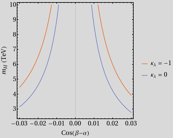
One can easily check that $\kappa_{\lambda}=1$, as expected in the limit $\alpha=\beta-\pi/2$. Currently the bound on $\kappa_{\lambda}$ is quite weak[11, 12]. Note that, the values of $m_{h}$ and $\beta$, appearing on the right hand side of Eq. (33), are known in our model. Therefore, assuming that $\cos(\beta-\alpha)$ and $\kappa_{\lambda}$ settle for some nonstandard values, we can predict the value of $m_{H}$. This feature has been illustrated in Fig. 1, where we can see that if, for example, the values of $\cos(\beta-\alpha)$ and $\kappa_{\lambda}$ are found to be $0.025$ and $-1$ respectively, then we can conclude that there should be a heavy neutral scalar appearing at around $5$ TeV. Although probing such a tiny value of $\cos(\beta-\alpha)$ might be an ambitious task for the near future, our model, nevertheless, exemplifies how the Higgs precision measurements can play a crucial role in pinning down the scale of new physics.

To summarize, in this article we have pointed out an intriguing possibility that there might be a connection between the Cabibbo angle and $\tan\beta$ in a 2HDM. To our knowledge, such a possibility has not been emphasized earlier in the context of 2HDMs. We accomplish this in a 2HDM with a $D_{4}$ symmetry which is only softly broken in the scalar potential. Because of the small number of Yukawa parameters, all the FCNC couplings are completely determined in our model. Additionally, the FCNC couplings are sufficiently small so that relatively light scalars accessible at the colliders can successfully negotiate the flavor constraints. Although the complete CKM matrix and the exact nonzero masses of the first generation of quarks have not been reproduced in our minimalistic scenario, we believe that the interesting features of this model outweigh the dissatisfaction with the small parameters in the quark sector. Perhaps the present framework can be taken as the first step towards a more complete theoretical construction which can address the full structure of the quark masses and mixings. Finally, it should be noted that, although there are quite a few previous examples of the use of $D_{4}$ symmetry to understand the leptonic sector[13, 14, 15, 16, 17, 18], instances where $D_{4}$ symmetry has been employed to explain the quark masses and mixings are rare[16, 19] and use four Higgs-doublets. Therefore, the current paper should be considered as a simpler alternative and an interesting addition to the existing literature on model building using $D_{4}$ flavor symmetry.

References

- [1] G. C. Branco, P. M. Ferreira, L. Lavoura, M. N. Rebelo, M. Sher, and J. P. Silva, Theory and phenomenology of two-Higgs-doublet models, Phys. Rept. 516 (2012) 1–102, [arXiv:1106.0034].
- [2] G. Bhattacharyya and D. Das, Scalar sector of two-Higgs-doublet models: A minireview, Pramana 87 (2016), no. 3 40, [arXiv:1507.06424].
- [3] H. Ishimori, T. Kobayashi, H. Ohki, Y. Shimizu, H. Okada, and M. Tanimoto, Non-Abelian Discrete Symmetries in Particle Physics, Prog. Theor. Phys. Suppl. 183 (2010) 1–163, [arXiv:1003.3552].
- [4] P. B. Pal, Symmetries of Regular Geometrical Objects, p. 281–310. Cambridge University Press, 2019.
- [5] J. F. Gunion and H. E. Haber, The CP conserving two Higgs doublet model: The Approach to the decoupling limit, Phys. Rev. D67 (2003) 075019, [hep-ph/0207010].
- [6] D. Das and I. Saha, Search for a stable alignment limit in two-Higgs-doublet models, Phys. Rev. D91 (2015), no. 9 095024, [arXiv:1503.02135].
- [7] P. S. Bhupal Dev and A. Pilaftsis, Maximally Symmetric Two Higgs Doublet Model with Natural Standard Model Alignment, JHEP 12 (2014) 024, [arXiv:1408.3405]. [Erratum: JHEP11,147(2015)].
- [8] W. Grimus, L. Lavoura, O. M. Ogreid, and P. Osland, A Precision constraint on multi-Higgs-doublet models, J. Phys. G35 (2008) 075001, [arXiv:0711.4022].
- [9] G. Bhattacharyya, D. Das, P. B. Pal, and M. N. Rebelo, Scalar sector properties of two-Higgs-doublet models with a global U(1) symmetry, JHEP 10 (2013) 081, [arXiv:1308.4297].
- [10] O. U. Shanker, Flavor Violation, Scalar Particles and Leptoquarks, Nucl. Phys. B206 (1982) 253–272.
- [11] CMS Collaboration, A. M. Sirunyan et al., Combination of searches for Higgs boson pair production in proton-proton collisions at 13 TeV, Phys. Rev. Lett. 122 (2019), no. 12 121803, [arXiv:1811.09689].
- [12] ATLAS Collaboration, Combination of searches for Higgs boson pairs in collisions at 13 TeV with the ATLAS experiment., Tech. Rep. ATLAS-CONF-2018-043, CERN, Geneva, Sep, 2018.
- [13] A. Adulpravitchai, A. Blum, and C. Hagedorn, A Supersymmetric D4 Model for mu-tau Symmetry, JHEP 03 (2009) 046, [arXiv:0812.3799].
- [14] H. Ishimori, T. Kobayashi, H. Ohki, Y. Omura, R. Takahashi, and M. Tanimoto, D(4) Flavor Symmetry for Neutrino Masses and Mixing, Phys. Lett. B662 (2008) 178–184, [arXiv:0802.2310].
- [15] C. Hagedorn and R. Ziegler, Symmetry and Charged Lepton Mass Hierarchy in a Supersymmetric Model, Phys. Rev. D82 (2010) 053011, [arXiv:1007.1888].
- [16] D. Meloni, S. Morisi, and E. Peinado, Stability of dark matter from the D4xZ2 flavor group, Phys. Lett. B703 (2011) 281–287, [arXiv:1104.0178].
- [17] V. V. Vien, Neutrino mass and mixing in the 3-3-1 model with neutral leptons based on D4 flavor symmetry, Mod. Phys. Lett. A29 (2014) 1450122.
- [18] V. V. Vien and H. N. Long, The flavor symmery in 3-3-1 model with neutral leptons, Int. J. Mod. Phys. A28 (2013) 1350159, [arXiv:1312.5034].
- [19] V. V. Vien and H. N. Long, Quark Masses and Mixings in an Extension of the Standard Model with D4 Flavor Symmetry, Phys. Atom. Nucl. 81 (2018), no. 6 750–757.