跳到论文正文
W Papers独立论文阅读器 arXiv:1908.03853 论文正文 计算阅读时间 · 0%
引用这篇论文根据当前论文元数据生成,正式投稿前建议核对。


License: arXiv.org perpetual non-exclusive license
arXiv:1908.03853v1 [math.AP] 11 Aug 2019

AN ASYMPTOTICALLY COMPATIBLE APPROACH FOR NEUMANN-TYPE BOUNDARY CONDITION ON NONLOCAL PROBLEMS

Abstract

In this paper we consider 2D nonlocal diffusion models with a finite nonlocal horizon parameter δ\delta characterizing the range of nonlocal interactions, and consider the treatment of Neumann-like boundary conditions that have proven challenging for discretizations of nonlocal models. While existing 2D nonlocal flux boundary conditions have been shown to exhibit at most first order convergence to the local counter part as δ→0\delta\rightarrow 0, we present a new generalization of classical local Neumann conditions that recovers the local case as O⁡(δ2)O(\delta^{2}) in the L∞​(Ω)L^{\infty}(\Omega) norm. This convergence rate is optimal considering the O⁡(δ2)O(\delta^{2}) convergence of the nonlocal equation to its local limit away from the boundary. We analyze the application of this new boundary treatment to the nonlocal diffusion problem, and present conditions under which the solution of the nonlocal boundary value problem converges to the solution of the corresponding local Neumann problem as the horizon is reduced. To demonstrate the applicability of this nonlocal flux boundary condition to more complicated scenarios, we extend the approach to less regular domains, numerically verifying that we preserve second-order convergence for domains with corners. Based on the new formulation for nonlocal boundary condition, we develop an asymptotically compatible meshfree discretization, obtaining a solution to the nonlocal diffusion equation with mixed boundary conditions that converges with O⁡(δ2)O(\delta^{2}) convergence.

Huaiqian You, Department of Mathematics, Lehigh University, Bethlehem, PA, USA
Xin Yang Lu, Department of Mathematical Sciences, Lakehead University, Thunder Bay, ON, Canada
Nathaniel Trask, Center for Computing Research, Sandia National Laboratories, Albuquerque, NM, USA
Yue Yu, Department of Mathematics, Lehigh University, Bethlehem, PA, USA, yuy214@lehigh.edu

Keywords. Integro-Differential Equations; Nonlocal Diffusion; Neumann-type Boundary Condition; Meshless; Asymptotic Compatibility.

AMS subject classifications. 45K05, 76R50, 65R20, 65G99.

1 Background

In recent years, there has been great interest in using nonlocal integro-differential equations (IDEs) as a means to describe physical systems, due to their natural ability to describe physical phenomena at small scales and their reduced regularity requirements which lead to greater flexibility [54, 8, 64, 29, 30, 63, 27, 25, 49, 42, 41, 13, 22, 18, 37, 24, 3, 17, 52, 14, 31]. In particular, nonlocal problems with Neumann-type boundary constraints have received particular attention [15, 16, 20, 34, 47, 7, 21, 23, 26, 55, 51, 1, 46, 63] due to their prevalence in describing problems related to: interfaces [2], free boundaries, and multiscale/multiphysics coupling problems [38, 53, 62, 5, 6]. Unlike classical PDE models, in the nonlocal IDEs the boundary conditions must be defined on a region with non-zero volume outside the surface [16, 21, 55], in contrast to more traditional engineering scenarios where boundary conditions are typically imposed on a sharp co-dimension one surface. Therefore, theoretical and numerical challenges arise from how to mathematically impose inhomogeneous Neumann-type boundary conditions properly in the nonlocal model. For instance, in the peridynamic theory of solid mechanics [54, 33, 19, 4, 61, 59, 32, 39, 28, 36, 40, 56], the classical description of material deformation locally via a deformation gradient is replaced by a nonlocal interaction described with integral operators. In these models, it has been shown that the careless imposition of traction conditions on the nonlocal boundary induces an unphysical strain energy concentration, leading in turn to the material being softer near the boundary. Such artificial phenomena are referred to in the literature as a "surface" or "skin" effect[35, 10].

A key feature in the discretization of nonlocal models has been the concept of asymptotic compatibility, originally introduced by Tian and Du [57], which describes the ability of a nonlocal discretization to recover a corresponding local model as both δ\delta and a characteristic discretization lengthscale are reduced at the same rate. We advocate the development of both nonlocal boundary treatment and discretization with the objective of preserving this limit. In so doing, we ensure that nonlocal models recover a well-understood classical limit, avoiding phenomena such as the surface effect. To this end, we introduce here a non-local boundary treatment that is designed to recover the classical theory. After rigorously proving that this nonlocal boundary value problem recovers the desired local Neumann problem as δ→0\delta\rightarrow 0, we have a firm mathematical foundation upon which to demonstrate asymptotic compatibility, where we will develop an asymptotically compatible numerical method and demonstrate its high-order convergence and a lack of artificial surface phenomena.

In this paper we study compactly supported nonlocal integro-differential equations (IDEs) with radial kernels. For concreteness, we focus on the nonlocal diffusion equation

Lδuδ:=−2∫B⁡(𝐱,δ)Jδ(|𝐱−𝐲|)(uδ(𝐲)−uδ(𝐱))d𝐲=f(𝐱),𝐱∈Ω⊂ℝN,L_{\delta}u_{\delta}:=-2\int_{B(\mathbf{x},\delta)}J_{\delta}(|\mathbf{x}-\mathbf{y}|)(u_{\delta}(\mathbf{y})-u_{\delta}(\mathbf{x}))d\mathbf{y}=f(\mathbf{x}),\quad\mathbf{x}\in\Omega\subset\mathbb{R}^{N}, (1.1)

although the proposed technique is applicable to more general problems. Here B⁡(𝐱,δ)B(\mathbf{x},\delta) is the ball centered at 𝐱\mathbf{x} with radius δ\delta, uδ​(𝐱)u_{\delta}(\mathbf{x}) is the solution, Ω\Omega is a bounded and connected domain in ℝN\mathbb{R}^{N} (N=2N=2), f⁡(𝐱)f(\mathbf{x}) is given data, and the kernel function Jδ:ℝ→ℝJ_{\delta}:\mathbb{R}\rightarrow\mathbb{R} is parameterized by a positive horizon parameter δ\delta which measures the extent of nonlocal interaction. We further take a popular choice of JδJ_{\delta} as a rescaled kernel given by

Jδ​(|𝝃|)=cδN+2​J​(|𝝃|δ),J_{\delta}(|\bm{\xi}|)=\dfrac{c}{\delta^{N+2}}J\left(\dfrac{|\bm{\xi}|}{\delta}\right), (1.2)

where J:[0,∞)→ℝJ:[0,\infty)\rightarrow\mathbb{R} is a nonnegative and continuous function with ∫ℝNJ⁡(|𝐳|)​|𝐳|2​𝑑𝐳=N\int_{\mathbb{R}^{N}}J(|\mathbf{z}|)|\mathbf{z}|^{2}d\mathbf{z}=N, ∫ℝNJ⁡(|𝐳|)​|𝐳|k​𝑑𝐳=o⁡(1)\int_{\mathbb{R}^{N}}J(|\mathbf{z}|)|\mathbf{z}|^{k}d\mathbf{z}=o(1) for all k≥3k\geq 3. Similar as in [55], we also assume that J⁡(r)J(r) is nonincreasing in rr, strictly positive in r∈[0,1]r\in[0,1] and vanishes when r>1r>1. In this work we aim to design a new formulation of Neumann-type constraint for the nonlocal problem (1.1) with mixed boundary conditions of Dirichlet, Neumann and mixed type, and present a numerical discretization of the resulting problem.

We pose three requirements for this formulation:

  1. 1.

    The constraint should be a proper nonlocal analogue to the local Neumann-type boundary conditions, so the formulation provides an approximation of physical boundary conditions on a sharp surface.

  2. 2.

    A boundary value problem given by the nonlocal Neumann-type constraint with the nonlocal diffusion equation (1.1) should be well-posed. Rigorous mathematical analysis on the existence, uniqueness and continuous dependence on data should be addressed for the associated variational problem.

  3. 3.

    The nonlocal Neumann-type boundary value problem should recover the classical Neumann problem as δ→0\delta\rightarrow 0, preferably with an optimal convergence rate of O​(δ2)\textit{O}(\delta^{2}) in the L∞L^{\infty} norm.

In the first part of the paper, we provide analysis of the boundary value problem (BVP) to establish the consistency and well-posedness of the boundary value problem. We establish here second-order convergence on non-trivial geometry, improving upon the first-order, one-dimensional analysis found in the literature.[16, 23, 55]. In the second part of this paper, we will present a new asymptotically compatible meshfree discretization of the proposed nonlocal BVP [9, 48, 58]. We pursue an extension of previous work by Trask et al. [58] utilizing an optimization-based approach to meshfree quadrature. This framework is attractive due to its demonstrated ability to achieve high-order asymptotically compatible solutions on unstructured data, which is complementary to the objective of developing boundary conditions consistent for irregular geometries. By introducing the new boundary treatment we will demonstrate improved second-order convergence over the previously demonstrated first order-convergence shown for Neumann problems [58].

The paper is organized as follows. We first present in Section 2 a definition of the nonlocal Neumann-type boundary condition and the corresponding nonlocal variational problem, together with the associated nonlocal operator and natural energy space. In Section 3, we study the well-posedness of the nonlocal variational problem for convex and sufficiently regular domains. We provide a consistency result for the nonlocal BVP by showing that the weak solution of the proposed nonlocal Neumann-type constrained value problem (denoted as uδu_{\delta}) converges to the solution of the corresponding classical diffusion problem (denoted as u0u_{0}) as the interaction horizon δ→0\delta\rightarrow 0 in the L2​(Ω)L^{2}(\Omega) norm. Although the main proof in this section has assumed homogeneous Neumann boundary conditions, a discussion on the extension to inhomogeneous Neumann-type boundary condition is also provided. Furthermore, in Section 4 we prove the O⁡(δ2)O(\delta^{2}) convergence rate of the continuous nonlocal solution uδu_{\delta} to u0u_{0} in the L∞​(Ω)L^{\infty}(\Omega) norm without extra regularity assumptions on uδu_{\delta}. Numerical results utilizing a meshfree quadrature rule are presented in Section 5. To verify the asymptotic compatibility of the combined boundary treatment and the meshfree numerical scheme, in Section 6 we use manufactured solutions to demonstrate the convergence of the discrete model to the local solution as both the discretization length scale hh and the nonlocal interaction length scale δ→0\delta\rightarrow 0. Furthermore, in Section 7 we extend the approach to domains with corners which indicate that the conclusions of the model problem and the convergence rates extrapolate to nontrivial problems of interest to the broader engineering community. Section 8 summarizes our findings and discusses future research. The appendices include additional technical details on the theoretical analysis.

2 A Nonlocal Flux Condition for 2D Diffusion Problem

Refer to caption
Refer to caption
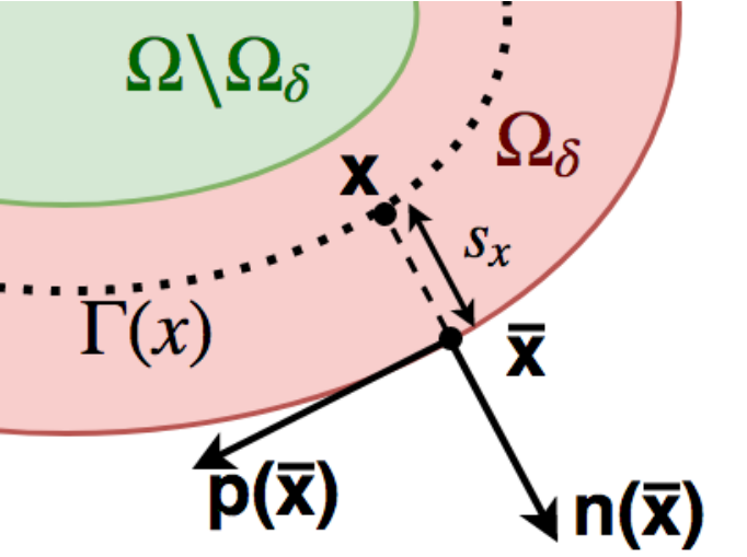
Figure 1: Left: Notations for the domain, where Ω\Omega is represented by the green and red regions together, and the nonlocal Neumann boundary condition is applied on the red region Ωδ\Omega_{\delta}. Right: Notations for the projection of point 𝐱∈Ωδ\mathbf{x}\in\Omega_{\delta}, the corresponding unit tangential vector 𝐩⁡(𝐱¯)\mathbf{p}(\overline{\mathbf{x}}) and the unit normal vector 𝐧⁡(𝐱¯)\mathbf{n}(\overline{\mathbf{x}}).

In this section, we first introduce a nonlocal flux boundary condition, and then provide a corresponding nonlocal variational problem along with the associated energy space for the purpose of analysis. Given that Ω∈ℝN\Omega\in\mathbb{R}^{N} (N=2)(N=2) is a bounded, convex, connected and C3C^{3} domain, we seek a nonlocal analogue to the local Neumann boundary condition ∂u∂𝐧=g⁡(𝐱)\dfrac{\partial u}{\partial\mathbf{n}}=g(\mathbf{x}), 𝐱∈∂Ω\mathbf{x}\in\partial\Omega in the following classical problem

{L0​u0:=−△​u0=f⁡(𝐱), in ​Ω∂u0∂𝐧=g⁡(𝐱), on ​∂Ω∫Ωu0​(𝐱)​d𝐱=0.\left\{\begin{array}[]{cl}L_{0}u_{0}:=-\triangle u_{0}=f(\mathbf{x}),&\text{ in }\Omega\\ \dfrac{\partial u_{0}}{\partial\mathbf{n}}=g(\mathbf{x}),&\text{ on }\partial\Omega\\ \\ \int_{\Omega}u_{0}(\mathbf{x})d\mathbf{x}=0.\\ \end{array}\right. (2.1)

Here 𝐧⁡(𝐱)\mathbf{n}({\mathbf{x}}) is the unit exterior normal to Ω\Omega at 𝐱{\mathbf{x}}. Moreover, we will use 𝐩⁡(𝐱)\mathbf{p}({\mathbf{x}}) to represent the unit tangential vector with orientation clockwise to 𝐧⁡(𝐱)\mathbf{n}({\mathbf{x}}). Before introducing our nonlocal formulation, we denote the following notation (see Figure 1 for illustration)

Ωδ:={𝐱∈Ω|dist​(𝐱,∂Ω)<δ},(ℝN\Ω)δ:={𝐱∈ℝN\Ω|dist​(𝐱,∂Ω)<δ}.\displaystyle\Omega_{\delta}:=\{\mathbf{x}\in\Omega|\text{dist}(\mathbf{x},\partial\Omega)<\delta\},\quad(\mathbb{R}^{N}\backslash\Omega)_{\delta}:=\{\mathbf{x}\in\mathbb{R}^{N}\backslash\Omega|\text{dist}(\mathbf{x},\partial\Omega)<\delta\}.

We further assume sufficient regularity in the boundary that we may take δ\delta sufficiently small so that for any 𝐱∈Ωδ\mathbf{x}\in\Omega_{\delta}, there exists a unique orthogonal projection of 𝐱\mathbf{x} onto ∂Ω\partial\Omega. We denote this projection as 𝐱¯\overline{\mathbf{x}}. Therefore, one has 𝐱¯−𝐱=sx​𝐧​(𝐱¯)\overline{\mathbf{x}}-\mathbf{x}=s_{x}\mathbf{n}(\overline{\mathbf{x}}) for 𝐱∈Ωδ\mathbf{x}\in\Omega_{\delta}, where 0<sx<δ0<s_{x}<\delta. We also assume that for 𝐱∈Ωδ\mathbf{x}\in\Omega_{\delta}, we can find a contour Γ⁡(𝐱)\Gamma(\mathbf{x}) which is parallel to ∂Ω\partial\Omega. In the following contents, we denote 𝐱l\mathbf{x}_{l} as the point with distance ll to 𝐱\mathbf{x} along Γ⁡(𝐱)\Gamma(\mathbf{x}) following the 𝐩⁡(𝐱¯)\mathbf{p}(\overline{\mathbf{x}}) direction, and 𝐱−l\mathbf{x}_{-l} as the point with distance ll to 𝐱\mathbf{x} in the opposite direction. Moreover, we employ the following notations for the directional components of the Hessian matrix of a scalar function vv:

[v⁡(𝐱)]p​p:=𝐩T​(𝐱¯)​∇2v​(𝐱)​𝐩​(𝐱¯),[v⁡(𝐱)]n​n:=𝐧T​(𝐱¯)​∇2v​(𝐱)​𝐧​(𝐱¯),[v⁡(𝐱)]p​n:=𝐩T​(𝐱¯)​∇2v​(𝐱)​𝐧​(𝐱¯),\displaystyle[v({{\mathbf{x}}})]_{pp}:=\mathbf{p}^{T}(\overline{\mathbf{x}})\nabla^{2}v({{\mathbf{x}}})\mathbf{p}(\overline{\mathbf{x}}),\quad[v({{\mathbf{x}}})]_{nn}:=\mathbf{n}^{T}(\overline{\mathbf{x}})\nabla^{2}v({{\mathbf{x}}})\mathbf{n}(\overline{\mathbf{x}}),\quad[v({{\mathbf{x}}})]_{pn}:=\mathbf{p}^{T}(\overline{\mathbf{x}})\nabla^{2}v({{\mathbf{x}}})\mathbf{n}(\overline{\mathbf{x}}),

and the higher order derivative components are similarly defined.

Since B⁡(𝐱,δ)∩(ℝN\Ω)δ≠∅B(\mathbf{x},\delta)\cap(\mathbb{R}^{N}\backslash\Omega)_{\delta}\neq\emptyset for 𝐱∈Ωδ\mathbf{x}\in\Omega_{\delta}, from (1.1) we have

Lδ​uδ=\displaystyle L_{\delta}u_{\delta}= −2∫B⁡(𝐱,δ)Jδ(|𝐱−𝐲|)(uδ(𝐲)−uδ(𝐱))d𝐲\displaystyle-2\int_{B(\mathbf{x},\delta)}J_{\delta}(|\mathbf{x}-\mathbf{y}|)(u_{\delta}(\mathbf{y})-u_{\delta}(\mathbf{x}))d\mathbf{y}
=\displaystyle= −2∫B⁡(𝐱,δ)∩ΩJδ(|𝐱−𝐲|)(uδ(𝐲)−uδ(𝐱))d𝐲−2∫B⁡(𝐱,δ)∩(ℝN\Ω)δJδ(|𝐱−𝐲|)(uδ(𝐲)−uδ(𝐱))d𝐲,\displaystyle-2\int_{B(\mathbf{x},\delta)\cap\Omega}J_{\delta}(|\mathbf{x}-\mathbf{y}|)(u_{\delta}(\mathbf{y})-u_{\delta}(\mathbf{x}))d\mathbf{y}-2\int_{B(\mathbf{x},\delta)\cap(\mathbb{R}^{N}\backslash\Omega)_{\delta}}J_{\delta}(|\mathbf{x}-\mathbf{y}|)(u_{\delta}(\mathbf{y})-u_{\delta}(\mathbf{x}))d\mathbf{y},

hence we need to approximate the integral in B⁡(𝐱,δ)∩(ℝN\Ω)δB(\mathbf{x},\delta)\cap(\mathbb{R}^{N}\backslash\Omega)_{\delta} and obtain a formulation with correction terms. Specifically, we propose the following flux boundary condition for (1.1): for 𝐱∈Ωδ\mathbf{x}\in\Omega_{\delta}

−2∫ΩJδ(|𝐱−𝐲|)(uδ(𝐲)−uδ(𝐱))d𝐲−∫ℝN\ΩJδ(|𝐱−𝐲|)(𝐲−𝐱)⋅𝐧(𝐱¯)(g(𝐱)+g(𝐲))d𝐲\displaystyle-2\int_{\Omega}J_{\delta}(|\mathbf{x}-\mathbf{y}|)(u_{\delta}(\mathbf{y})-u_{\delta}(\mathbf{x}))d\mathbf{y}-\int_{\mathbb{R}^{N}\backslash\Omega}J_{\delta}(|\mathbf{x}-\mathbf{y}|)(\mathbf{y}-\mathbf{x})\cdot\mathbf{n}(\overline{\mathbf{x}})(g({\mathbf{x}})+g({\mathbf{y}}))d\mathbf{y}
−∫ℝN\ΩJδ(|𝐱−𝐲|)|(𝐲−𝐱)⋅𝐩(𝐱¯)|2d𝐲[uδ(𝐱)]p​p=f(𝐱),\displaystyle-\int_{\mathbb{R}^{N}\backslash\Omega}J_{\delta}(|\mathbf{x}-\mathbf{y}|)|(\mathbf{y}-\mathbf{x})\cdot\mathbf{p}(\overline{\mathbf{x}})|^{2}d\mathbf{y}[u_{\delta}({{\mathbf{x}}})]_{pp}=f(\mathbf{x}), (2.2)

where the second and third terms aim to provide an approximation for

−2∫ℝN\ΩJδ(|𝐱−𝐲|)(uδ(𝐲)−uδ(𝐱))d𝐲.-2\int_{\mathbb{R}^{N}\backslash\Omega}J_{\delta}(|\mathbf{x}-\mathbf{y}|)(u_{\delta}(\mathbf{y})-u_{\delta}(\mathbf{x}))d\mathbf{y}.

Since the boundary condition g⁡(𝐱)g(\mathbf{x}) is defined only on ∂Ω\partial\Omega, the g⁡(𝐱)g(\mathbf{x}) and g⁡(𝐲)g(\mathbf{y}) terms in (2.2) will be approximated with the following (local) extensions

g⁡(𝐱)≈g⁡(𝐱¯)−(𝐱−𝐱¯)⋅𝐧⁡(𝐱¯)​f​(𝐱)−(𝐱−𝐱¯)⋅𝐧⁡(𝐱¯)​[uδ​(𝐱)]p​p,\displaystyle g(\mathbf{x})\approx g(\overline{\mathbf{x}})-(\mathbf{x}-\overline{\mathbf{x}})\cdot\mathbf{n}(\overline{\mathbf{x}})f({{\mathbf{x}}})-(\mathbf{x}-\overline{\mathbf{x}})\cdot\mathbf{n}(\overline{\mathbf{x}})[u_{\delta}({{\mathbf{x}}})]_{pp},
g⁡(𝐲)≈g⁡(𝐱¯)−(𝐲−𝐱¯)⋅𝐧⁡(𝐱¯)​f​(𝐱)−(𝐲−𝐱¯)⋅𝐧⁡(𝐱¯)​[uδ​(𝐱)]p​p.\displaystyle g(\mathbf{y})\approx g(\overline{\mathbf{x}})-(\mathbf{y}-\overline{\mathbf{x}})\cdot\mathbf{n}(\overline{\mathbf{x}})f({{\mathbf{x}}})-(\mathbf{y}-\overline{\mathbf{x}})\cdot\mathbf{n}(\overline{\mathbf{x}})[u_{\delta}({{\mathbf{x}}})]_{pp}.

Furthermore, we replace [uδ​(𝐱)]p​p[u_{\delta}({{\mathbf{x}}})]_{pp} with its approximation 2​∫−δδHδ​(|l|)​(uδ​(𝐱l)−uδ​(𝐱))​d​𝐱l−κ⁡(𝐱¯)​g​(𝐱¯)2\int_{-\delta}^{\delta}H_{\delta}(|l|)(u_{\delta}(\mathbf{x}_{l})-u_{\delta}(\mathbf{x}))d\mathbf{x}_{l}-\kappa(\overline{\mathbf{x}})g(\overline{\mathbf{x}}), where d​𝐱ld\mathbf{x}_{l} is the line integral along the contour Γ⁡(𝐱)\Gamma(\mathbf{x}), κ⁡(𝐱¯)\kappa(\overline{\mathbf{x}}) is the curvature of ∂Ω\partial\Omega at 𝐱¯\overline{\mathbf{x}}, and Hδ​(|r|)=cδ3​H​(|r|δ)H_{\delta}(|r|)=\dfrac{c}{\delta^{3}}H\left(\dfrac{|r|}{\delta}\right) is the kernel for 1D nonlocal diffusion model. Similar to the requirements for JJ, we assume here H:[0,∞)→ℝH:[0,\infty)\rightarrow\mathbb{R} to be a nonnegative and continuous function with ∫ℝH⁡(|z|)​|z|2​𝑑z=1\int_{\mathbb{R}}H(|z|)|z|^{2}dz=1, ∫ℝH⁡(|z|)​|z|k​𝑑z=o⁡(1)\int_{\mathbb{R}}H(|z|)|z|^{k}dz=o(1) for all k≥3k\geq 3. H⁡(r)H(r) is nonincreasing in rr, strictly positive in [0,1][0,1] and vanishes for |z|>1|z|>1. Moreover, we add a further requirement on HH that ∫ℝH⁡(z)​𝑑z:=CH<∞\int_{\mathbb{R}}H(z)dz:=C_{H}<\infty. Here we note that 2​∫−δδHδ​(|l|)​(uδ​(𝐱l)−uδ​(𝐱))​d​𝐱l2\int_{-\delta}^{\delta}H_{\delta}(|l|)(u_{\delta}(\mathbf{x}_{l})-u_{\delta}(\mathbf{x}))d\mathbf{x}_{l} is a nonlocal version of the Laplace-Beltrami operator defined on Γ⁡(𝐱)\Gamma(\mathbf{x}). Substituting the above two approximations into (2.2), we obtain the following model

−2∫ΩJδ(|𝐱−𝐲|)(uδ(𝐲)−uδ(𝐱))d𝐲−2Mδ(𝐱)∫−δδHδ(|l|)(uδ(𝐱l)−uδ(𝐱))d𝐱l\displaystyle-2\int_{\Omega}J_{\delta}(|\mathbf{x}-\mathbf{y}|)(u_{\delta}(\mathbf{y})-u_{\delta}(\mathbf{x}))d\mathbf{y}-2M_{\delta}(\mathbf{x})\int_{-\delta}^{\delta}H_{\delta}(|l|)(u_{\delta}(\mathbf{x}_{l})-u_{\delta}(\mathbf{x}))d\mathbf{x}_{l}
=\displaystyle= f⁡(𝐱)−∫ℝN\ΩJδ​(|𝐱−𝐲|)​[|(𝐲−𝐱¯)⋅𝐧⁡(𝐱¯)|2−|(𝐱−𝐱¯)⋅𝐧⁡(𝐱¯)|2]​𝑑𝐲​f​(𝐱)\displaystyle f({{\mathbf{x}}})-\int_{\mathbb{R}^{N}\backslash\Omega}J_{\delta}(|\mathbf{x}-\mathbf{y}|)\left[|(\mathbf{y}-\overline{\mathbf{x}})\cdot\mathbf{n}(\overline{\mathbf{x}})|^{2}-|(\mathbf{x}-\overline{\mathbf{x}})\cdot\mathbf{n}(\overline{\mathbf{x}})|^{2}\right]d\mathbf{y}f({{\mathbf{x}}})
+(2​∫ℝN\ΩJδ​(|𝐱−𝐲|)​(𝐲−𝐱)⋅𝐧⁡(𝐱¯)​𝑑𝐲−Mδ​(𝐱)​κ​(𝐱¯))​g​(𝐱¯).\displaystyle+\left(2\int_{\mathbb{R}^{N}\backslash\Omega}J_{\delta}(|\mathbf{x}-\mathbf{y}|)(\mathbf{y}-\mathbf{x})\cdot\mathbf{n}(\overline{\mathbf{x}})d\mathbf{y}-M_{\delta}(\mathbf{x})\kappa(\overline{\mathbf{x}})\right)g(\overline{\mathbf{x}}). (2.3)

where

Mδ​(𝐱):=∫ℝN\ΩJδ​(|𝐱−𝐲|)​[|(𝐲−𝐱)⋅𝐩⁡(𝐱¯)|2−|(𝐲−𝐱¯)⋅𝐧⁡(𝐱¯)|2+|(𝐱−𝐱¯)⋅𝐧⁡(𝐱¯)|2]​𝑑𝐲.M_{\delta}(\mathbf{x}):=\int_{\mathbb{R}^{N}\backslash\Omega}J_{\delta}(|\mathbf{x}-\mathbf{y}|)\left[|(\mathbf{y}-\mathbf{x})\cdot\mathbf{p}(\overline{\mathbf{x}})|^{2}-|(\mathbf{y}-\overline{\mathbf{x}})\cdot\mathbf{n}(\overline{\mathbf{x}})|^{2}+|(\mathbf{x}-\overline{\mathbf{x}})\cdot\mathbf{n}(\overline{\mathbf{x}})|^{2}\right]d\mathbf{y}.

Thus, by defining the nonlocal operator

LN​δ​u:=\displaystyle L_{N\delta}u:= −2∫ΩJδ(|𝐱−𝐲|)(u(𝐲)−u(𝐱))d𝐲−2Mδ(𝐱)∫−δδHδ(|l|)(u(𝐱l)−u(𝐱))d𝐱l\displaystyle-2\int_{\Omega}J_{\delta}(|\mathbf{x}-\mathbf{y}|)(u(\mathbf{y})-u(\mathbf{x}))d\mathbf{y}-2M_{\delta}(\mathbf{x}){\int_{-\delta}^{\delta}H_{\delta}(|l|)(u(\mathbf{x}_{l})-u(\mathbf{x}))d\mathbf{x}_{l}}

and

fδ​(𝐱):=\displaystyle{f}_{\delta}(\mathbf{x}):= f⁡(𝐱)−∫ℝN\ΩJδ​(|𝐱−𝐲|)​[|(𝐲−𝐱¯)⋅𝐧⁡(𝐱¯)|2−|(𝐱−𝐱¯)⋅𝐧⁡(𝐱¯)|2]​𝑑𝐲​f​(𝐱)\displaystyle f({{\mathbf{x}}})-\int_{\mathbb{R}^{N}\backslash\Omega}J_{\delta}(|\mathbf{x}-\mathbf{y}|)\left[|(\mathbf{y}-\overline{\mathbf{x}})\cdot\mathbf{n}(\overline{\mathbf{x}})|^{2}-|(\mathbf{x}-\overline{\mathbf{x}})\cdot\mathbf{n}(\overline{\mathbf{x}})|^{2}\right]d\mathbf{y}f({{\mathbf{x}}})
+(2​∫ℝN\ΩJδ​(|𝐱−𝐲|)​(𝐲−𝐱)⋅𝐧⁡(𝐱¯)​𝑑𝐲−Mδ​(𝐱)​κ​(𝐱¯))​g​(𝐱¯),\displaystyle+\left(2\int_{\mathbb{R}^{N}\backslash\Omega}J_{\delta}(|\mathbf{x}-\mathbf{y}|)(\mathbf{y}-\mathbf{x})\cdot\mathbf{n}(\overline{\mathbf{x}})d\mathbf{y}-M_{\delta}(\mathbf{x})\kappa(\overline{\mathbf{x}})\right)g(\overline{\mathbf{x}}), (2.4)

the proposed algorithm is equivalent to the following nonlocal integral equation

{LN​δ​uδ=fδ, in ​Ω∫Ωuδ​d𝐱=0.\left\{\begin{array}[]{cl}L_{N\delta}u_{\delta}=f_{\delta},&\text{ in }\Omega\\ \int_{\Omega}u_{\delta}d\mathbf{x}=0.&\\ \end{array}\right. (2.5)

The corresponding nonlocal weak formulation can then be introduced

Bδ​(uδ,v)=(fδ,v)L2​(Ω),B_{\delta}(u_{\delta},v)=({f}_{\delta},v)_{L^{2}(\Omega)}, (2.6)

where Bδ​(u,v)B_{\delta}(u,v) denotes a nonsymmetric bilinear form Bδ​(u,v):=(Lδ​u,v)B_{\delta}(u,v):=(L_{\delta}u,v). We note that

−2∫Ω∫ΩJδ(|𝐱−𝐲|)(u(𝐲)−u(𝐱))d𝐲v(𝐱)d𝐱\displaystyle-2\int_{\Omega}\int_{\Omega}J_{\delta}(|\mathbf{x}-\mathbf{y}|)(u(\mathbf{y})-u(\mathbf{x}))d\mathbf{y}v(\mathbf{x})d\mathbf{x}
=\displaystyle= −∫Ω∫ΩJδ(|𝐱−𝐲|)(u(𝐲)−u(𝐱))v(𝐱)d𝐲d𝐱−∫Ω∫ΩJδ(|𝐲−𝐱|)(u(𝐱)−u(𝐲))v(𝐲)d𝐲d𝐱\displaystyle-\int_{\Omega}\int_{\Omega}J_{\delta}(|\mathbf{x}-\mathbf{y}|)(u(\mathbf{y})-u(\mathbf{x}))v(\mathbf{x})d\mathbf{y}d\mathbf{x}-\int_{\Omega}\int_{\Omega}J_{\delta}(|\mathbf{y}-\mathbf{x}|)(u(\mathbf{x})-u(\mathbf{y}))v(\mathbf{y})d\mathbf{y}d\mathbf{x}
=\displaystyle= ∫Ω∫ΩJδ​(|𝐱−𝐲|)​[u⁡(𝐲)−u⁡(𝐱)]​[v⁡(𝐲)−v⁡(𝐱)]​𝑑𝐲​𝑑𝐱\displaystyle\int_{\Omega}\int_{\Omega}J_{\delta}(|\mathbf{x}-\mathbf{y}|)[u(\mathbf{y})-u(\mathbf{x})][v(\mathbf{y})-v(\mathbf{x})]d\mathbf{y}d\mathbf{x}

and

−2∫ΩMδ(𝐱)∫−δδHδ(|l|)(u(𝐱l)−u(𝐱))d𝐱lv(𝐱)d𝐱\displaystyle-2\int_{\Omega}M_{\delta}(\mathbf{x}){\int_{-\delta}^{\delta}H_{\delta}(|l|)(u(\mathbf{x}_{l})-u(\mathbf{x}))d\mathbf{x}_{l}}v(\mathbf{x})d\mathbf{x}
=\displaystyle= −2∫Ω∫ΩMδ(𝐱)Hδ(|l|)D(𝐱,𝐲)(u(𝐲)−u(𝐱))v(𝐱)d𝐲d𝐱\displaystyle-2\int_{\Omega}\int_{\Omega}M_{\delta}(\mathbf{x})H_{\delta}(|l|)D(\mathbf{x},\mathbf{y})(u(\mathbf{y})-u(\mathbf{x}))v(\mathbf{x})d\mathbf{y}d\mathbf{x}
=\displaystyle= ∫Ω∫ΩMδ​(𝐱)​Hδ​(|l|)​D​(𝐱,𝐲)​(u⁡(𝐲)−u⁡(𝐱))​[v⁡(𝐲)−v⁡(𝐱)]​𝑑𝐲​𝑑𝐱\displaystyle\int_{\Omega}\int_{\Omega}M_{\delta}(\mathbf{x})H_{\delta}(|l|)D(\mathbf{x},\mathbf{y})(u(\mathbf{y})-u(\mathbf{x}))[v(\mathbf{y})-v(\mathbf{x})]d\mathbf{y}d\mathbf{x}
−∫Ω∫ΩMδ(𝐲)Hδ(|l|)D(𝐲,𝐱)(u(𝐱)−u(𝐲))v(𝐱)d𝐱d𝐲\displaystyle-\int_{\Omega}\int_{\Omega}M_{\delta}(\mathbf{y})H_{\delta}(|l|)D(\mathbf{y},\mathbf{x})(u(\mathbf{x})-u(\mathbf{y}))v(\mathbf{x})d\mathbf{x}d\mathbf{y}
−∫Ω∫ΩMδ(𝐱)Hδ(|l|)D(𝐱,𝐲)(u(𝐲)−u(𝐱))v(𝐱)d𝐲d𝐱\displaystyle-\int_{\Omega}\int_{\Omega}M_{\delta}(\mathbf{x})H_{\delta}(|l|)D(\mathbf{x},\mathbf{y})(u(\mathbf{y})-u(\mathbf{x}))v(\mathbf{x})d\mathbf{y}d\mathbf{x}
=\displaystyle= ∫Ω∫ΩMδ​(𝐱)​Hδ​(|l|)​D​(𝐱,𝐲)​[u⁡(𝐲)−u⁡(𝐱)]​[v⁡(𝐲)−v⁡(𝐱)]​|𝐫′​(𝐲)|​𝑑𝐲​𝑑𝐱\displaystyle\int_{\Omega}\int_{\Omega}M_{\delta}(\mathbf{x})H_{\delta}(|l|)D(\mathbf{x},\mathbf{y})[u(\mathbf{y})-u(\mathbf{x})][v(\mathbf{y})-v(\mathbf{x})]|\mathbf{r}^{\prime}(\mathbf{y})|d\mathbf{y}d\mathbf{x}
+∫Ω∫Ω[Mδ(𝐲)|𝐫′​(𝐱)||𝐫′​(𝐲)|−Mδ(𝐱)]Hδ(|l|)D(𝐱,𝐲)(u(𝐲)−u(𝐱))v(𝐱)|𝐫′(𝐲)|d𝐲d𝐱\displaystyle+\int_{\Omega}\int_{\Omega}\left[M_{\delta}(\mathbf{y})\dfrac{|\mathbf{r}^{\prime}(\mathbf{x})|}{|\mathbf{r}^{\prime}(\mathbf{y})|}-M_{\delta}(\mathbf{x})\right]H_{\delta}(|l|)D(\mathbf{x},\mathbf{y})(u(\mathbf{y})-u(\mathbf{x}))v(\mathbf{x})|\mathbf{r}^{\prime}(\mathbf{y})|d\mathbf{y}d\mathbf{x}
=\displaystyle= ∫ΩδMδ​(𝐱)​∫−δδHδ​(|l|)​[u⁡(𝐱l)−u⁡(𝐱)]​[v⁡(𝐱l)−v⁡(𝐱)]​d​𝐱l​𝑑𝐱\displaystyle\int_{\Omega_{\delta}}M_{\delta}(\mathbf{x})\int_{-\delta}^{\delta}H_{\delta}(|l|)[u(\mathbf{x}_{l})-u(\mathbf{x})][v(\mathbf{x}_{l})-v(\mathbf{x})]d\mathbf{x}_{l}d\mathbf{x}
+∫Ωδ∫−δδ[Mδ(𝐱l)|𝐫′​(𝐱)||𝐫′​(𝐱l)|−Mδ(𝐱)]Hδ(|l|)[u(𝐱l)−u(𝐱)]d𝐱lv(𝐱)d𝐱,\displaystyle+\int_{\Omega_{\delta}}\int_{-\delta}^{\delta}\left[M_{\delta}(\mathbf{x}_{l})\dfrac{|\mathbf{r}^{\prime}(\mathbf{x})|}{|\mathbf{r}^{\prime}(\mathbf{x}_{l})|}-M_{\delta}(\mathbf{x})\right]H_{\delta}(|l|)[u(\mathbf{x}_{l})-u(\mathbf{x})]d\mathbf{x}_{l}v(\mathbf{x})d\mathbf{x},

where 𝐫\mathbf{r} is the bijective parametrization of Γ⁡(𝐱)\Gamma(\mathbf{x}), |𝐫′​(𝐱)||\mathbf{r}^{\prime}(\mathbf{x})| is the Jacobian of 𝐫\mathbf{r}, and D⁡(𝐱,𝐲)D(\mathbf{x},\mathbf{y}) denotes a Dirac-Delta function:

D⁡(𝐱,𝐲):=limϵ→0ϵ−1​ψ​(dist​(𝐲,Γ⁡(𝐱))/ϵ),where ​ψ​ is a mollifier function on ​ℝ.D(\mathbf{x},\mathbf{y}):=\lim_{\epsilon\rightarrow 0}\epsilon^{-1}\psi(\text{dist}(\mathbf{y},\Gamma(\mathbf{x}))/\epsilon),\;\text{where }\psi\text{ is a mollifier function on }\mathbb{R}.

Therefore

Bδ​(u,v)=\displaystyle B_{\delta}(u,v)= ∫Ω∫ΩJδ​(|𝐱−𝐲|)​[u⁡(𝐲)−u⁡(𝐱)]​[v⁡(𝐲)−v⁡(𝐱)]​𝑑𝐲​𝑑𝐱\displaystyle\int_{\Omega}\int_{\Omega}J_{\delta}(|\mathbf{x}-\mathbf{y}|)[u(\mathbf{y})-u(\mathbf{x})][v(\mathbf{y})-v(\mathbf{x})]d\mathbf{y}d\mathbf{x}
+∫ΩδMδ(𝐱)∫−δδHδ(|l|)[u(𝐱l)−u(𝐱)][v(𝐱l)−v(𝐱)]d𝐱ld𝐱\displaystyle+\int_{\Omega_{\delta}}M_{\delta}(\mathbf{x})\int_{-\delta}^{\delta}H_{\delta}(|l|)[u(\mathbf{x}_{l})-u(\mathbf{x})][v(\mathbf{x}_{l})-v(\mathbf{x})]d\mathbf{x}_{l}d\mathbf{x}
+∫Ωδ∫−δδ[Mδ(𝐱l)|𝐫′​(𝐱)||𝐫′​(𝐱l)|−Mδ(𝐱)]Hδ(|l|)[u(𝐱l)−u(𝐱)]d𝐱lv(𝐱)d𝐱.\displaystyle+\int_{\Omega_{\delta}}\int_{-\delta}^{\delta}\left[M_{\delta}(\mathbf{x}_{l})\dfrac{|\mathbf{r}^{\prime}(\mathbf{x})|}{|\mathbf{r}^{\prime}(\mathbf{x}_{l})|}-M_{\delta}(\mathbf{x})\right]H_{\delta}(|l|)[u(\mathbf{x}_{l})-u(\mathbf{x})]d\mathbf{x}_{l}v(\mathbf{x})d\mathbf{x}. (2.7)

We then consider the nonlocal energy seminorm ||⋅||Sδ||\cdot||_{S_{\delta}} as

‖u‖Sδ2=\displaystyle||u||^{2}_{S_{\delta}}= ∫Ω∫ΩJδ​(|𝐱−𝐲|)​[u⁡(𝐲)−u⁡(𝐱)]2​𝑑𝐲​𝑑𝐱+∫ΩδMδ​(𝐱)​∫−δδHδ​(|l|)​[u⁡(𝐱l)−u⁡(𝐱)]2​d​𝐱l​𝑑𝐱,\displaystyle\int_{\Omega}\int_{\Omega}J_{\delta}(|\mathbf{x}-\mathbf{y}|)[u(\mathbf{y})-u(\mathbf{x})]^{2}d\mathbf{y}d\mathbf{x}+\int_{\Omega_{\delta}}M_{\delta}(\mathbf{x})\int_{-\delta}^{\delta}H_{\delta}(|l|)[u(\mathbf{x}_{l})-u(\mathbf{x})]^{2}d\mathbf{x}_{l}d\mathbf{x},

with corresponding constrained energy space given by

Sδ(Ω)={u∈L2(Ω):||u||Sδ<∞,∫Ωud𝐱=0}.S_{\delta}(\Omega)=\left\{u\in L^{2}(\Omega):||u||_{S_{\delta}}<\infty,\,\int_{\Omega}ud\mathbf{x}=0\right\}.

Given the nonlocal Poincare inequality which will be addressed in the next section, we will see that ||⋅||Sδ||\cdot||_{S_{\delta}} is actually a full norm. Similar to [44], one can show that the constrained energy space Sδ​(Ω)S_{\delta}(\Omega) is a Hilbert space under the given assumptions for the kernels JJ and HH.

Remark 2.1.

A similar form of the flux condition (2.2) has been proposed in the previous literature, e.g., [16, 55]. By comparing the second term of (2.2) with the first case in [16], one can see that the second term of (2.2) can be obtained by taking G=G1G=G_{1} in [16] and modifying the correction term ∫ℝN\ΩGδ​(𝐱,𝐱−𝐲)​g​(𝐲)​𝑑𝐲\int_{\mathbb{R}^{N}\backslash\Omega}G_{\delta}(\mathbf{x},\mathbf{x}-\mathbf{y})g({\mathbf{y}})d\mathbf{y} as ∫ℝN\ΩGδ​(𝐱,𝐱−𝐲)​12​(g⁡(𝐱)+g⁡(𝐲))​𝑑𝐲\int_{\mathbb{R}^{N}\backslash\Omega}G_{\delta}(\mathbf{x},\mathbf{x}-\mathbf{y})\dfrac{1}{2}(g({\mathbf{x}})+g({\mathbf{y}}))d\mathbf{y}. Actually, this modification is sufficient to provide a nonlocal Neumann-type condition with second order accuracy in the 1D case, as shown in [55]. However, in higher dimensional cases we need to add the third term of (2.2) to achieve second order accuracy.

Remark 2.2.

Note that in the current paper we focus on the 2​D2D nonlocal diffusion problem, while the idea can be further extended to the 3​D3D cases and to more general nonlocal IDEs, which will be addressed in future work.

3 Well-Posedness and Asymptotic Property

In this section, we first address the well-posedness of the proposed nonlocal Neumann volume-constrained problem by providing a nonlocal Poincaré-type inequality based on the estimates for boundary curvature κ⁡(𝐱)\kappa(\mathbf{x}) and its derivative κ′​(𝐱)\kappa^{\prime}(\mathbf{x}). The coercivity and boundedness of the nonsymmetric bilinear operator Bδ​(⋅,⋅)B_{\delta}(\cdot,\cdot) defined in (2.7) follow, which yield the well-posedness of the variational problem. Furthermore, we study the consistency of the nonlocal problem with the classical local model. Specifically, following the framework introduced in [57] we prove the uniform embedding property and the precompact property of the proposed norm SδS_{\delta}, and then show the asymptotic property of the solution of (2.5) as δ→0\delta\rightarrow 0, i.e., the solution uδu_{\delta} converges to the solution u0u_{0} from the limiting local model (2.1). Here for simplicity we consider the case when g⁡(𝐱)=0g(\mathbf{x})=0, and defer discussion of inhomogeneous boundary conditions until Remark 3.11. For the limiting local model one can define the corresponding inner product ‖u‖S0=‖∇u‖L2​(Ω)||u||_{S_{0}}=||\nabla u||_{L^{2}(\Omega)}, the bilinear form B0​(u,v)=(∇u,∇v)B_{0}(u,v)=(\nabla u,\nabla v) and the constrained energy space S0={u∈H1​(Ω):∫Ωu​𝑑𝐱=0}S_{0}=\left\{u\in H^{1}(\Omega):\int_{\Omega}ud\mathbf{x}=0\right\}. Throughout this section, we consider the symbol “CC” to indicate a generic constant that is independent of δ\delta, but may have different numerical values in different situations. Moreover, we introduce the following notation for simplicity:

bδ​(u,v)\displaystyle b_{\delta}(u,v) :=∫Ω∫ΩJδ​(|𝐱−𝐲|)​(u⁡(𝐲)−u⁡(𝐱))​(v⁡(𝐲)−v⁡(𝐱))​𝑑𝐲​𝑑𝐱,\displaystyle:=\int_{\Omega}\int_{\Omega}J_{\delta}(|\mathbf{x}-\mathbf{y}|)(u(\mathbf{y})-u(\mathbf{x}))(v(\mathbf{y})-v(\mathbf{x}))d\mathbf{y}d\mathbf{x},
hδ​(u,v)\displaystyle h_{\delta}(u,v) :=∫ΩδMδ​(𝐱)​∫−δδHδ​(|l|)​[u⁡(𝐱l)−u⁡(𝐱)]​[v⁡(𝐱l)−v⁡(𝐱)]​d​𝐱l​𝑑𝐱,\displaystyle:={\int_{\Omega_{\delta}}M_{\delta}(\mathbf{x})\int_{-\delta}^{\delta}H_{\delta}(|l|)[u(\mathbf{x}_{l})-u(\mathbf{x})][v(\mathbf{x}_{l})-v(\mathbf{x})]d\mathbf{x}_{l}d\mathbf{x}},
Iδ​(𝐱,𝐲)\displaystyle I_{\delta}(\mathbf{x},\mathbf{y}) :=|(𝐲−𝐱)⋅𝐩⁡(𝐱¯)|2−|(𝐲−𝐱¯)⋅𝐧⁡(𝐱¯)|2+|(𝐱−𝐱¯)⋅𝐧⁡(𝐱¯)|2.\displaystyle:=|(\mathbf{y}-\mathbf{x})\cdot\mathbf{p}(\overline{\mathbf{x}})|^{2}-|(\mathbf{y}-\overline{\mathbf{x}})\cdot\mathbf{n}(\overline{\mathbf{x}})|^{2}+|(\mathbf{x}-\overline{\mathbf{x}})\cdot\mathbf{n}(\overline{\mathbf{x}})|^{2}.

We first have the following estimates of the function Mδ​(𝐱)M_{\delta}(\mathbf{x}) for each 𝐱∈Ωδ\mathbf{x}\in\Omega_{\delta}:

Lemma 3.1.

For l∈[−δ,δ]l\in[-\delta,\delta], and assuming that there exist constants d,D>0d,D>0 such that |κ′​(𝐳)|≤D|\kappa^{\prime}(\mathbf{z})|\leq D, |κ⁡(𝐳)|≤D|\kappa(\mathbf{z})|\leq D and sup|ξ|≤d|κ′​(𝐳ξ)κ⁡(𝐳)|≤D\sup_{|\xi|\leq d}\left|\dfrac{\kappa^{\prime}(\mathbf{z}_{\xi})}{\kappa(\mathbf{z})}\right|\leq D for almost every 𝐳∈∂Ω\mathbf{z}\in\partial\Omega, there exists a 0<δ¯≤d0<\overline{\delta}\leq d such that for δ≤δ¯\delta\leq\overline{\delta} for almost every 𝐱∈∂Ω\mathbf{x}\in\partial\Omega we have 0≤Mδ​(𝐱)≤C0\leq M_{\delta}(\mathbf{x})\leq C and

|Mδ​(𝐱)−Mδ​(𝐱l)​|𝐫′​(𝐱)||𝐫′​(𝐱l)||≤CM​δ2,\left|M_{\delta}(\mathbf{x})-M_{\delta}(\mathbf{x}_{l})\dfrac{|\mathbf{r}^{\prime}(\mathbf{x})|}{|\mathbf{r}^{\prime}(\mathbf{x}_{l})|}\right|\leq C_{M}\delta^{2}, (3.1)
|Mδ​(𝐱)​|𝐫′​(𝐱l)|−Mδ​(𝐱l)​|𝐫′​(𝐱)|Mδ​(𝐱)​|𝐫′​(𝐱l)||≤CN​δ,\bigg|\frac{M_{\delta}(\mathbf{x})|\mathbf{r}^{\prime}(\mathbf{x}_{l})|-M_{\delta}(\mathbf{x}_{l})|\mathbf{r}^{\prime}(\mathbf{x})|}{M_{\delta}(\mathbf{x})|\mathbf{r}^{\prime}(\mathbf{x}_{l})|}\bigg|\leq C_{N}\delta, (3.2)

where CMC_{M}, CNC_{N} are constants independent of δ\delta.

Proof.

Figure 2: Notation for the geometric estimates in Lemma 3.1. Left: illustration of regions DδD_{\delta} and AδA_{\delta}. Green represents DδD_{\delta}, the region in B⁡(𝐱,δ)B(\mathbf{x},\delta) which lies on the other side of the tangential line at 𝐱¯\overline{\mathbf{x}} with respect to Ω\Omega. Cyan represents AδA_{\delta}, the region in B⁡(𝐱,δ)B(\mathbf{x},\delta) which lies between ∂Ω\partial\Omega and the tangential line. Right: Representation of the Cartesian coordinate system locally near 𝐱¯\overline{\mathbf{x}}. Here the region AδA_{\delta} lies below the red curve y=f⁡(x)y=f(x).

We show now that 0≤Mδ​(𝐱)≤C0\leq M_{\delta}(\mathbf{x})\leq C. Note that

Mδ​(𝐱)=∫(ℝN\Ω)δJδ​(|𝐱−𝐲|)​Iδ​𝑑𝐲=∫DδJδ​(|𝐱−𝐲|)​Iδ​𝑑𝐲+∫AδJδ​(|𝐱−𝐲|)​Iδ​𝑑𝐲.M_{\delta}(\mathbf{x})=\int_{(\mathbb{R}^{N}\backslash\Omega)_{\delta}}J_{\delta}(|\mathbf{x}-\mathbf{y}|)I_{\delta}d\mathbf{y}=\int_{D_{\delta}}J_{\delta}(|\mathbf{x}-\mathbf{y}|)I_{\delta}d\mathbf{y}+\int_{A_{\delta}}J_{\delta}(|\mathbf{x}-\mathbf{y}|)I_{\delta}d\mathbf{y}.

With τ⁡(𝐱¯)\tau(\overline{\mathbf{x}}) representing the tangent line to ∂Ω\partial\Omega at 𝐱¯\overline{\mathbf{x}}, here DδD_{\delta} is the region of B⁡(𝐱,δ)B(\mathbf{x},\delta) on the side of τ⁡(𝐱¯)\tau(\overline{\mathbf{x}}) not containing Ω\Omega (as shown in the green region in the left plot of Figure 2), and Aδ:=B⁡(𝐱,δ)\(Dδ∪Ω)A_{\delta}:=B(\mathbf{x},\delta)\backslash(D_{\delta}\cup\Omega) (as shown in the cyan region in the left plot of Figure 2). We consider first the DδD_{\delta} part. One can rewrite 𝐲∈Dδ\mathbf{y}\in D_{\delta} as 𝐱+(r​cos⁡(θ),r​sin⁡(θ))\mathbf{x}+(r\cos(\theta),r\sin(\theta)) with sx<r<δs_{x}<r<\delta and −π/2<−arccos(sx/r)≤θ≤arccos(sx/r)≤π/2-\pi/2<-\arccos(s_{x}/r)\leq\theta\leq\arccos(s_{x}/r)\leq\pi/2, which yields

∫DδJδ​(|𝐱−𝐲|)​Iδ​𝑑𝐲\displaystyle\int_{D_{\delta}}J_{\delta}(|\mathbf{x}-\mathbf{y}|)I_{\delta}d\mathbf{y} =∫sxδJδ​(r)​∫−arccos⁡(sx/r)arccos⁡(sx/r)Iδ​(𝐱,𝐲)​r​𝑑θ​𝑑r\displaystyle=\int_{s_{x}}^{\delta}J_{\delta}(r)\int_{-\arccos(s_{x}/r)}^{\arccos(s_{x}/r)}I_{\delta}(\mathbf{x},\mathbf{y})rd\theta dr
=2​∫sxδJδ​(r)​r2​1−(sx/r)2​sx​𝑑r.\displaystyle=2\int_{s_{x}}^{\delta}J_{\delta}(r)r^{2}\sqrt{1-(s_{x}/r)^{2}}s_{x}dr. (3.3)

From (3.3) we can see that ∫DδJδ​(|𝐱−𝐲|)​Iδ​𝑑𝐲≥0\int_{D_{\delta}}J_{\delta}(|\mathbf{x}-\mathbf{y}|)I_{\delta}d\mathbf{y}\geq 0 and

Mδ​(𝐱)\displaystyle M_{\delta}(\mathbf{x}) ≥∫AδJδ​(|𝐱−𝐲|)​[|(𝐲−𝐱¯)⋅𝐩⁡(𝐱¯)|2−|(𝐲−𝐱¯)⋅𝐧⁡(𝐱¯)|2]​𝑑𝐲.\displaystyle\geq\int_{A_{\delta}}J_{\delta}(|\mathbf{x}-\mathbf{y}|)[|(\mathbf{y}-\overline{\mathbf{x}})\cdot\mathbf{p}(\overline{\mathbf{x}})|^{2}-|(\mathbf{y}-\overline{\mathbf{x}})\cdot\mathbf{n}(\overline{\mathbf{x}})|^{2}]d\mathbf{y}. (3.4)

Therefore it suffices to show now that

|(𝐲−𝐱¯)⋅𝐩⁡(𝐱¯)|≥|(𝐲−𝐱¯)⋅𝐧⁡(𝐱¯)|∀𝐲∈Aδ.|(\mathbf{y}-\overline{\mathbf{x}})\cdot\mathbf{p}(\overline{\mathbf{x}})|\geq|(\mathbf{y}-\overline{\mathbf{x}})\cdot\mathbf{n}(\overline{\mathbf{x}})|\qquad\forall\mathbf{y}\in A_{\delta}. (3.5)

We adopt a Cartesian coordinate system as shown in the right plot of Figure 2, assuming that 𝐱¯\overline{\mathbf{x}} coincides with the origin, 𝐩⁡(𝐱¯)\mathbf{p}(\overline{\mathbf{x}}) is oriented along the positive direction of the xx-axis while 𝐧⁡(𝐱¯)\mathbf{n}(\overline{\mathbf{x}}) coincides with the negative direction of the yy-axis. We then have 𝐱¯=(0,0)\overline{\mathbf{x}}=(0,0), τ(𝐱¯)={y=0}\tau(\overline{\mathbf{x}})=\{y=0\}, Ω⊆{y≥0}\Omega\subseteq\{y\geq 0\}, and let y=f⁡(x)y=f(x) be the curve describing ∂Ω\partial\Omega. We note that any point 𝐲\mathbf{y} lying below y=|x|y=|x| satisfies (3.5). Assuming that there exists a point 𝐳∈∂Ω\mathbf{z}\in\partial\Omega lying above y=|x|y=|x|, there exists x0≠0x_{0}\neq 0 such that f⁡(x0)=|x0|f(x_{0})=|x_{0}| and (x0,f⁡(x0))∈∂Ω(x_{0},f(x_{0}))\in\partial\Omega. For simplicity we consider the case where x0>0x_{0}>0 since the case where x0<0x_{0}<0 is analogous. Since f′​(0)=0f^{\prime}(0)=0, by continuity there exists at least one point x1∈(0,x0)x_{1}\in(0,x_{0}) such that f′​(x1)≥1f^{\prime}(x_{1})\geq 1. Let x2:=inf{t>0:f′​(t)≥1}≤x1≤x0x_{2}:=\inf\{t>0:f^{\prime}(t)\geq 1\}\leq x_{1}\leq x_{0}, then by the regularity of ff we have x2>0x_{2}>0. Thus f′​(x2)−f′​(0)=1=∫0x2f′′​(s)​𝑑sf^{\prime}(x_{2})-f^{\prime}(0)=1=\int_{0}^{x_{2}}f^{\prime\prime}(s)ds. Moreover, the unsigned curvature of the graph of ff can be given by |f′′(x)|(1+f′(x)2)−3/2|f^{\prime\prime}(x)|(1+f^{\prime}(x)^{2})^{-3/2}. Due to the finiteness of the curvature of ∂Ω\partial\Omega, and the fact that f′​(x)2≤1f^{\prime}(x)^{2}\leq 1 for all x∈[0,x2]x\in[0,x_{2}], we obtain D≥|f′′(x)|(1+f′(x)2)−3/2D\geq|f^{\prime\prime}(x)|(1+f^{\prime}(x)^{2})^{-3/2} and therefore

|f′′​(x)|≤D​(1+f′​(x)2)3/2≤2​2​D,∀x∈[0,x2].\displaystyle|f^{\prime\prime}(x)|\leq D(1+f^{\prime}(x)^{2})^{3/2}\leq 2\sqrt{2}D,\qquad\forall x\in[0,x_{2}].

Hence

1\displaystyle 1 =∫0x2f′′​(s)​𝑑s≤∫0x2|f′′​(s)|​𝑑s≤2​2​x2​D⇒x2≥12​2​D.\displaystyle=\int_{0}^{x_{2}}f^{\prime\prime}(s)ds\leq\int_{0}^{x_{2}}|f^{\prime\prime}(s)|ds\leq 2\sqrt{2}x_{2}D\Rightarrow x_{2}\geq\frac{1}{2\sqrt{2}D}.

But since x2≤x0x_{2}\leq x_{0}, this means that the first intersection point between y=f⁡(x)y=f(x) and y=|x|y=|x| (which we denote as 𝐰=(x0,|x0|)\mathbf{w}=(x_{0},|x_{0}|)) has distance at least x2x_{2} from 𝐱¯=(0,0)\overline{\mathbf{x}}=(0,0). Thus, for sufficiently small δ≤14​2​D=:δ1\delta\leq\frac{1}{4\sqrt{2}D}=:\delta_{1}, we get

|𝐰−𝐱¯|\displaystyle|\mathbf{w}-\overline{\mathbf{x}}| ≥x2≥12​2​D≥2​δ=supp,q∈B⁡(𝐱,δ)|p−q|.\displaystyle\geq x_{2}\geq\frac{1}{2\sqrt{2}D}\geq 2\delta=\sup_{p,q\in B(\mathbf{x},\delta)}|p-q|.

Therefore, 𝐰∉B⁡(𝐱,δ)\mathbf{w}\notin B(\mathbf{x},\delta), and the entire region AδA_{\delta} lies below y=|x|y=|x|. Consequently, any 𝐲∈Aδ\mathbf{y}\in A_{\delta} satisfies |(𝐲−𝐱¯)⋅𝐩⁡(𝐱¯)|≥|(𝐲−𝐱¯)⋅𝐧⁡(𝐱¯)||(\mathbf{y}-\overline{\mathbf{x}})\cdot\mathbf{p}(\overline{\mathbf{x}})|\geq|(\mathbf{y}-\overline{\mathbf{x}})\cdot\mathbf{n}(\overline{\mathbf{x}})| and in turn Mδ≥0M_{\delta}\geq 0. On the other hand, with the C3C^{3} regularity of Ω\Omega and by Taylor expansion B⁡(𝐱,δ)∩∂ΩB(\mathbf{x},\delta)\cap\partial\Omega is the graph of a function of the form y=f⁡(x)=κ⁡(𝐱¯)2​x2+O⁡(x3)y=f(x)=\frac{\kappa(\overline{\mathbf{x}})}{2}x^{2}+O(x^{3}). Therefore, the area |Aδ|≤C​|κ⁡(𝐱¯)|​(δ2−sx2)3/2≤C​D​δ3|A_{\delta}|\leq C|\kappa(\overline{\mathbf{x}})|(\delta^{2}-s_{x}^{2})^{3/2}\leq CD\delta^{3}. Hence

Mδ​(𝐱)≤\displaystyle M_{\delta}(\mathbf{x})\leq |∫DδJδ​(|𝐱−𝐲|)​Iδ​𝑑𝐲|+|∫AδJδ​(|𝐱−𝐲|)​Iδ​𝑑𝐲|\displaystyle\left|\int_{D_{\delta}}J_{\delta}(|\mathbf{x}-\mathbf{y}|)I_{\delta}d\mathbf{y}\right|+\left|\int_{A_{\delta}}J_{\delta}(|\mathbf{x}-\mathbf{y}|)I_{\delta}d\mathbf{y}\right|
≤\displaystyle\leq C​suprJ⁡(|r|)​(δ−4​sx​(δ2−sx2)3/2+D​δ)≤C.\displaystyle C\sup_{r}J(|r|)(\delta^{-4}s_{x}(\delta^{2}-s_{x}^{2})^{3/2}+D\delta)\leq C.

To show (3.1), denoting by Dδ,𝐱l,Aδ,𝐱lD_{\delta,\mathbf{x}_{l}},A_{\delta,\mathbf{x}_{l}} the analogous sets of Dδ,AδD_{\delta},A_{\delta} at 𝐱l\mathbf{x}_{l} instead of 𝐱\mathbf{x}, we then have

Mδ​(𝐱)−Mδ​(𝐱l)​|𝐫′​(𝐱)||𝐫′​(𝐱l)|=\displaystyle M_{\delta}(\mathbf{x})-M_{\delta}(\mathbf{x}_{l})\dfrac{|\mathbf{r}^{\prime}(\mathbf{x})|}{|\mathbf{r}^{\prime}(\mathbf{x}_{l})|}= ∫DδJδ​(|𝐱−𝐲|)​Iδ​(𝐱,𝐲)​𝑑𝐲−|𝐫′​(𝐱)||𝐫′​(𝐱l)|​∫Dδ,𝐱lJδ​(|𝐱l−𝐲|)​Iδ​(𝐱l,𝐲)​𝑑𝐲\displaystyle\int_{D_{\delta}}J_{\delta}(|\mathbf{x}-\mathbf{y}|)I_{\delta}(\mathbf{x},\mathbf{y})d\mathbf{y}-\dfrac{|\mathbf{r}^{\prime}(\mathbf{x})|}{|\mathbf{r}^{\prime}(\mathbf{x}_{l})|}\int_{D_{\delta,\mathbf{x}_{l}}}J_{\delta}(|\mathbf{x}_{l}-\mathbf{y}|)I_{\delta}(\mathbf{x}_{l},\mathbf{y})d\mathbf{y}
+∫AδJδ(|𝐱−𝐲|)Iδ(𝐱,𝐲)d𝐲−|𝐫′​(𝐱)||𝐫′​(𝐱l)|∫Aδ,𝐱lJδ(|𝐱l−𝐲|)Iδ(𝐱l,𝐲)d𝐲.\displaystyle+\int_{A_{\delta}}J_{\delta}(|\mathbf{x}-\mathbf{y}|)I_{\delta}(\mathbf{x},\mathbf{y})d\mathbf{y}-\dfrac{|\mathbf{r}^{\prime}(\mathbf{x})|}{|\mathbf{r}^{\prime}(\mathbf{x}_{l})|}\int_{A_{\delta,\mathbf{x}_{l}}}J_{\delta}(|\mathbf{x}_{l}-\mathbf{y}|)I_{\delta}(\mathbf{x}_{l},\mathbf{y})d\mathbf{y}.

With the definition of 𝐱l\mathbf{x}_{l} and the regularity assumptions on Ω\Omega, it holds s𝐱l:=dist​(𝐱l,∂Ω)=dist​(𝐱,∂Ω)s_{\mathbf{x}_{l}}:=\text{dist}(\mathbf{x}_{l},\partial\Omega)=\text{dist}(\mathbf{x},\partial\Omega). We obtain

∫Dδ,𝐱lJδ​(|𝐱l−𝐲|)​Iδ​(𝐱l,𝐲)​𝑑𝐲=∫DδJδ​(|𝐱−𝐲|)​Iδ​(𝐱,𝐲)​𝑑𝐲.\int_{D_{\delta,\mathbf{x}_{l}}}J_{\delta}(|\mathbf{x}_{l}-\mathbf{y}|)I_{\delta}(\mathbf{x}_{l},\mathbf{y})d\mathbf{y}=\int_{D_{\delta}}J_{\delta}(|\mathbf{x}-\mathbf{y}|)I_{\delta}(\mathbf{x},\mathbf{y})d\mathbf{y}.

Moreover, with the coordinate system as shown in the right plot of Figure 2, we have |𝐫′​(𝐱)|=1|\mathbf{r}^{\prime}(\mathbf{x})|=1 and |𝐫′​(𝐱l)|=1+(f′​(x))2|\mathbf{r}^{\prime}(\mathbf{x}_{l})|=\sqrt{1+(f^{\prime}(x))^{2}}. Since for any point 𝐱l=(xl,f⁡(xl))\mathbf{x}_{l}=(x_{l},f(x_{l})) in B⁡(𝐱,δ)B(\mathbf{x},\delta), |f′​(xl)|=|xl​f′′​(ξ)|≤C​δ|f^{\prime}(x_{l})|=|x_{l}f^{\prime\prime}(\xi)|\leq C\delta for some ξ∈[0,xl]\xi\in[0,x_{l}], therefore

||𝐫′​(𝐱)||𝐫′​(𝐱l)|−1|=|11+(f′​(xl))2−1|=12​(f′​(xl))2+O⁡(δ4)≤C​δ2\left|\dfrac{|\mathbf{r}^{\prime}(\mathbf{x})|}{|\mathbf{r}^{\prime}(\mathbf{x}_{l})|}-1\right|=\left|\dfrac{1}{\sqrt{1+(f^{\prime}(x_{l}))^{2}}}-1\right|=\dfrac{1}{2}(f^{\prime}(x_{l}))^{2}+O(\delta^{4})\leq C\delta^{2} (3.6)

and hence together with (3.3) we obtain

∫DδJδ​(|𝐱−𝐲|)​Iδ​(𝐱,𝐲)​𝑑𝐲−|𝐫′​(𝐱)||𝐫′​(𝐱l)|​∫Dδ,𝐱lJδ​(|𝐱l−𝐲|)​Iδ​(𝐱l,𝐲)​𝑑𝐲≤C​δ2.\int_{D_{\delta}}J_{\delta}(|\mathbf{x}-\mathbf{y}|)I_{\delta}(\mathbf{x},\mathbf{y})d\mathbf{y}-\dfrac{|\mathbf{r}^{\prime}(\mathbf{x})|}{|\mathbf{r}^{\prime}(\mathbf{x}_{l})|}\int_{D_{\delta,\mathbf{x}_{l}}}J_{\delta}(|\mathbf{x}_{l}-\mathbf{y}|)I_{\delta}(\mathbf{x}_{l},\mathbf{y})d\mathbf{y}\leq C\delta^{2}.

To estimate ∫AδJδ​(|𝐱−𝐲|)​Iδ​(𝐱,𝐲)​𝑑𝐲−∫Aδ,𝐱lJδ​(|𝐱l−𝐲|)​Iδ​(𝐱l,𝐲)​𝑑𝐲\int_{A_{\delta}}J_{\delta}(|\mathbf{x}-\mathbf{y}|)I_{\delta}(\mathbf{x},\mathbf{y})d\mathbf{y}-\int_{A_{\delta,\mathbf{x}_{l}}}J_{\delta}(|\mathbf{x}_{l}-\mathbf{y}|)I_{\delta}(\mathbf{x}_{l},\mathbf{y})d\mathbf{y}, let RR be the rototranslation mapping such that

R⁡(𝐱¯l)=𝐱¯,R⁡(𝐩⁡(𝐱¯l))=𝐩⁡(𝐱¯),R⁡(𝐧⁡(𝐱¯l))=𝐧⁡(𝐱¯).R(\overline{\mathbf{x}}_{l})=\overline{\mathbf{x}},\quad R(\mathbf{p}(\overline{\mathbf{x}}_{l}))=\mathbf{p}(\overline{\mathbf{x}}),\quad R(\mathbf{n}(\overline{\mathbf{x}}_{l}))=\mathbf{n}(\overline{\mathbf{x}}).

With such construction we note that the curves R⁡(B⁡(𝐱l,δ)∩∂Ω)R(B({\mathbf{x}}_{l},\delta)\cap\partial\Omega) and B⁡(𝐱,δ)∩∂ΩB({\mathbf{x}},\delta)\cap\partial\Omega share the same tangential lines at 𝐱¯\overline{\mathbf{x}}. Meanwhile, B⁡(𝐱,δ)∩∂ΩB({\mathbf{x}},\delta)\cap\partial\Omega and R⁡(B⁡(𝐱l,δ)∩∂Ω)R(B({\mathbf{x}}_{l},\delta)\cap\partial\Omega) have different curvatures κ⁡(𝐱¯)\kappa(\overline{\mathbf{x}}) and κ⁡(𝐱¯l)\kappa(\overline{\mathbf{x}}_{l}), respectively. When δ≪1/D\delta\ll 1/D, we have the arc lengths of R⁡(B⁡(𝐱l,δ)∩∂Ω)R(B({\mathbf{x}}_{l},\delta)\cap\partial\Omega) and B⁡(𝐱,δ)∩∂ΩB({\mathbf{x}},\delta)\cap\partial\Omega satisfying |R⁡(B⁡(𝐱l,δ)∩∂Ω)|≤2​δ2−sx2+C​κ​(𝐱¯l)​(δ2−sx2)|R(B({\mathbf{x}}_{l},\delta)\cap\partial\Omega)|\leq 2\sqrt{\delta^{2}-s_{x}^{2}}+C\kappa(\overline{\mathbf{x}}_{l})(\delta^{2}-s_{x}^{2}) and |B⁡(𝐱,δ)∩∂Ω|≤2​δ2−sx2+C​κ​(𝐱¯)​(δ2−sx2)|B({\mathbf{x}},\delta)\cap\partial\Omega|\leq 2\sqrt{\delta^{2}-s_{x}^{2}}+C\kappa(\overline{\mathbf{x}})(\delta^{2}-s_{x}^{2}). Moreover, the spread dℋ​(B⁡(𝐱,δ)∩∂Ω,R⁡(B⁡(𝐱l,δ)∩∂Ω))d_{\mathcal{H}}(B({\mathbf{x}},\delta)\cap\partial\Omega,R(B({\mathbf{x}}_{l},\delta)\cap\partial\Omega)) is bounded by

dℋ​(B⁡(𝐱,δ)∩∂Ω,R⁡(B⁡(𝐱l,δ)∩∂Ω))\displaystyle d_{\mathcal{H}}(B({\mathbf{x}},\delta)\cap\partial\Omega,R(B({\mathbf{x}}_{l},\delta)\cap\partial\Omega))
=\displaystyle= max⁡{supz∈B⁡(𝐱,δ)∩∂Ωdist​(z,R⁡(B⁡(𝐱l,δ)∩∂Ω)),supz∈R⁡(B⁡(𝐱l,δ)∩∂Ω)dist​(z,B⁡(𝐱,δ)∩∂Ω)}\displaystyle\max\Big\{\sup_{z\in B({\mathbf{x}},\delta)\cap\partial\Omega}\text{dist}(z,R(B({\mathbf{x}}_{l},\delta)\cap\partial\Omega)),\sup_{z\in R(B({\mathbf{x}}_{l},\delta)\cap\partial\Omega)}\text{dist}(z,B({\mathbf{x}},\delta)\cap\partial\Omega)\Big\}
≤\displaystyle\leq C​|κ⁡(𝐱¯l)−κ⁡(𝐱¯)|​(δ2−sx2).\displaystyle C|\kappa(\overline{\mathbf{x}}_{l})-\kappa(\overline{\mathbf{x}})|(\delta^{2}-s_{x}^{2}).

Therefore, noting that the quantities JδJ_{\delta}, IδI_{\delta} and d​𝐲d\mathbf{y} are invariant under RR, and |Iδ​(𝐱l,𝐲)||I_{\delta}(\mathbf{x}_{l},\mathbf{y})|, |Iδ​(𝐱,𝐲)|≤3​δ2|I_{\delta}(\mathbf{x},\mathbf{y})|\leq 3\delta^{2}, one has

|∫Aδ,𝐱lJδ​(|𝐱l−𝐲|)​Iδ​(𝐱l,𝐲)​𝑑𝐲−∫AδJδ​(|𝐱−𝐲|)​Iδ​(𝐱,𝐲)​𝑑𝐲|\displaystyle\bigg|\int_{A_{\delta,\mathbf{x}_{l}}}J_{\delta}(|\mathbf{x}_{l}-\mathbf{y}|)I_{\delta}(\mathbf{x}_{l},\mathbf{y})d\mathbf{y}-\int_{A_{\delta}}J_{\delta}(|\mathbf{x}-\mathbf{y}|)I_{\delta}(\mathbf{x},\mathbf{y})d\mathbf{y}\bigg|
=\displaystyle= |∫R⁡(Aδ,𝐱l)Jδ​(|𝐱−𝐲|)​Iδ​(𝐱,𝐲)​𝑑𝐲−∫AδJδ​(|𝐱−𝐲|)​Iδ​(𝐱,𝐲)​𝑑𝐲|\displaystyle\bigg|\int_{R(A_{\delta,\mathbf{x}_{l}})}J_{\delta}(|\mathbf{x}-\mathbf{y}|)I_{\delta}(\mathbf{x},\mathbf{y})d\mathbf{y}-\int_{A_{\delta}}J_{\delta}(|\mathbf{x}-\mathbf{y}|)I_{\delta}(\mathbf{x},\mathbf{y})d\mathbf{y}\bigg|
≤\displaystyle\leq C​∫Aδ​Δ​R​(Aδ,𝐱l)Jδ​(|𝐱−𝐲|)​δ2​𝑑𝐲≤C​|κ⁡(𝐱¯l)−κ⁡(𝐱¯)|​δ−2​(δ2−sx2)3/2\displaystyle C\int_{A_{\delta}\Delta R(A_{\delta,\mathbf{x}_{l}})}J_{\delta}(|\mathbf{x}-\mathbf{y}|)\delta^{2}d\mathbf{y}\leq C|\kappa(\overline{\mathbf{x}}_{l})-\kappa(\overline{\mathbf{x}})|\delta^{-2}(\delta^{2}-s_{x}^{2})^{3/2}
≤\displaystyle\leq C​sup|ξ|≤|l||κ′​(𝐱¯ξ)|​δ−1​(δ2−sx2)3/2≤C​δ−1​(δ2−sx2)3/2,\displaystyle C\sup_{|\xi|\leq|l|}|\kappa^{\prime}(\overline{\mathbf{x}}_{\xi})|\delta^{-1}(\delta^{2}-s_{x}^{2})^{3/2}\leq C\delta^{-1}(\delta^{2}-s_{x}^{2})^{3/2}, (3.7)

where the constant CC depends on suprJ⁡(|r|)\sup_{r}J(|r|) and is independent of δ\delta. Moreover, with (3.6) and |∫AδJδ​(|𝐱−𝐲|)​Iδ​𝑑𝐲|≤C​suprJ⁡(|r|​δCLOSE\left|\int_{A_{\delta}}J_{\delta}(|\mathbf{x}-\mathbf{y}|)I_{\delta}d\mathbf{y}\right|\leq C\sup_{r}J(|r|\delta we have

|(1−|𝐫′​(𝐱)||𝐫′​(𝐱l)|)​∫Aδ,𝐱lJδ​(|𝐱l−𝐲|)​Iδ​(𝐱l,𝐲)​𝑑𝐲|≤C​δ3.\left|\left(1-\dfrac{|\mathbf{r}^{\prime}(\mathbf{x})|}{|\mathbf{r}^{\prime}(\mathbf{x}_{l})|}\right)\int_{A_{\delta,\mathbf{x}_{l}}}J_{\delta}(|\mathbf{x}_{l}-\mathbf{y}|)I_{\delta}(\mathbf{x}_{l},\mathbf{y})d\mathbf{y}\right|\leq C\delta^{3}.

Thus, we obtain the bound in (3.1).

We now work on the proof of (3.2) by combining (3.7) and establishing a lower bound for MδM_{\delta}. We firstly prove that

|Mδ​(𝐱)−Mδ​(𝐱l)Mδ​(𝐱)|≤C​δ.\bigg|\frac{M_{\delta}(\mathbf{x})-M_{\delta}(\mathbf{x}_{l})}{M_{\delta}(\mathbf{x})}\bigg|\leq C\delta. (3.8)

With the previous calculation, we have

∫DδJδ​(𝐱−𝐲)​Iδ​𝑑𝐲=2​∫sxδJδ​(r)​r2​1−(sx/r)2​sx​𝑑r≥C​δ−4​sx​(δ2−sx2)3/2\displaystyle\int_{D_{\delta}}J_{\delta}(\mathbf{x}-\mathbf{y})I_{\delta}d\mathbf{y}=2\int_{s_{x}}^{\delta}J_{\delta}(r)r^{2}\sqrt{1-(s_{x}/r)^{2}}s_{x}dr\geq C\delta^{-4}s_{x}(\delta^{2}-s_{x}^{2})^{3/2}
≥\displaystyle\geq CD|κ⁡(𝐱¯)|δ−4​sx​(δ2−sx2)3/2=C​|κ⁡(𝐱¯)|​δ−4​sx​(δ2−sx2)3/2\displaystyle\dfrac{C}{D}|\kappa(\overline{\mathbf{x}})|\delta^{-4}s_{x}(\delta^{2}-s_{x}^{2})^{3/2}=C|\kappa(\overline{\mathbf{x}})|\delta^{-4}s_{x}(\delta^{2}-s_{x}^{2})^{3/2}

and ∫AδJδ​(𝐱−𝐲)​Iδ​𝑑𝐲≥0\int_{A_{\delta}}J_{\delta}(\mathbf{x}-\mathbf{y})I_{\delta}d\mathbf{y}\geq 0. When sx2≥δ2/2s^{2}_{x}\geq\delta^{2}/2 one has

|Mδ​(𝐱)−Mδ​(𝐱l)Mδ​(𝐱)|≤\displaystyle\bigg|\frac{M_{\delta}(\mathbf{x})-M_{\delta}(\mathbf{x}_{l})}{M_{\delta}(\mathbf{x})}\bigg|\leq C​|κ⁡(𝐱¯l)−κ⁡(𝐱¯)|​δ−2​(δ2−sx2)3/2|κ⁡(𝐱¯)|​δ−4​sx​(δ2−sx2)3/2=C​δ3sx​sup|ξ|≤d|κ′​(𝐱¯ξ)κ⁡(𝐱¯)|≤C​δ​sup|ξ|≤d|κ′​(𝐱¯ξ)κ⁡(𝐱¯)|\displaystyle C\dfrac{|\kappa(\overline{\mathbf{x}}_{l})-\kappa(\overline{\mathbf{x}})|\delta^{-2}(\delta^{2}-s_{x}^{2})^{3/2}}{|\kappa(\overline{\mathbf{x}})|\delta^{-4}s_{x}(\delta^{2}-s_{x}^{2})^{3/2}}=C\dfrac{\delta^{3}}{s_{x}}\sup_{|\xi|\leq d}\left|\dfrac{\kappa^{\prime}(\overline{\mathbf{x}}_{\xi})}{\kappa(\overline{\mathbf{x}})}\right|\leq C\delta\sup_{|\xi|\leq d}\left|\dfrac{\kappa^{\prime}(\overline{\mathbf{x}}_{\xi})}{\kappa(\overline{\mathbf{x}})}\right|

and therefore (3.8) holds true. For sx2<δ2/2s^{2}_{x}<\delta^{2}/2, we just need to bound ∫AδJδ​(𝐱−𝐲)​Iδ​𝑑𝐲\int_{A_{\delta}}J_{\delta}(\mathbf{x}-\mathbf{y})I_{\delta}d\mathbf{y} from below. For notational simplicity, we assume here the Cartesian coordinate system shown in the right plot of Figure 2. The following properties hold:

(𝐲−𝐱¯)⋅𝐩⁡(𝐱¯)=x​ coordinate of ​𝐲,\displaystyle(\mathbf{y}-\overline{\mathbf{x}})\cdot\mathbf{p}(\overline{\mathbf{x}})=x\text{ coordinate of }\mathbf{y}, (3.9)
(𝐲−𝐱¯)⋅𝐧⁡(𝐱¯)=−(y​ coordinate of ​𝐲).\displaystyle\quad(\mathbf{y}-\overline{\mathbf{x}})\cdot\mathbf{n}(\overline{\mathbf{x}})=-(y\text{ coordinate of }\mathbf{y}). (3.10)

We first assume that |κ⁡(𝐱¯)|>0|\kappa(\overline{\mathbf{x}})|>0. By Taylor approximation, B⁡(𝐱,δ)∩∂ΩB(\mathbf{x},\delta)\cap\partial\Omega is the graph of a function of the form y=f⁡(x)=κ⁡(𝐱¯)2​x2+O⁡(x3)y=f(x)=\frac{\kappa(\overline{\mathbf{x}})}{2}x^{2}+O(x^{3}). Integrating it yields that the area |Aδ|=C|κ⁡(𝐱¯)|(δ2−sx2)3/2=C​|κ⁡(𝐱¯)|​δ3|A_{\delta}|=C|\kappa(\overline{\mathbf{x}})|(\delta^{2}-s_{x}^{2})^{3/2}=C|\kappa(\overline{\mathbf{x}})|\delta^{3}. Let h∈(0,1)h\in(0,1) be a point where the area of Aδ∩{x≥hδ}A_{\delta}\cap\{x\geq h\delta\} is C​|κ⁡(𝐱¯)|​δ3/2C|\kappa(\overline{\mathbf{x}})|\delta^{3}/2. With the convexity assumption of ∂Ω\partial\Omega, one has h>1/2h>1/2. When δ≤δ1<12​D\delta\leq\delta_{1}<\frac{1}{2D}, the slope of ff (i.e. the slope of the tangent derivative of B⁡(𝐱,δ)∩∂ΩB(\mathbf{x},\delta)\cap\partial\Omega) can reach at most δ​D<1/2\delta D<1/2. Thus the graph of ff lies below the line y=x/2y=x/2 and (3.10) gives

Iδ≥\displaystyle I_{\delta}\geq |(𝐲−𝐱)⋅𝐩⁡(𝐱¯)|2−|(𝐲−𝐱¯)⋅𝐧⁡(𝐱¯)|2≥|(𝐲−𝐱¯)⋅𝐩⁡(𝐱¯)|2−|(𝐲−𝐱¯)⋅𝐧⁡(𝐱¯)|2\displaystyle|(\mathbf{y}-\mathbf{x})\cdot\mathbf{p}(\overline{\mathbf{x}})|^{2}-|(\mathbf{y}-\overline{\mathbf{x}})\cdot\mathbf{n}(\overline{\mathbf{x}})|^{2}\geq|(\mathbf{y}-\overline{\mathbf{x}})\cdot\mathbf{p}(\overline{\mathbf{x}})|^{2}-|(\mathbf{y}-\overline{\mathbf{x}})\cdot\mathbf{n}(\overline{\mathbf{x}})|^{2}
≥\displaystyle\geq 34​|(𝐲−𝐱¯)⋅𝐩⁡(𝐱¯)|2≥34​h2​δ2≥316​δ2\displaystyle\frac{3}{4}|(\mathbf{y}-\overline{\mathbf{x}})\cdot\mathbf{p}(\overline{\mathbf{x}})|^{2}\geq\frac{3}{4}h^{2}\delta^{2}\geq\dfrac{3}{16}\delta^{2}

for all 𝐲∈Aδ∩{x≥hδ}\mathbf{y}\in A_{\delta}\cap\{x\geq h\delta\}. Recalling that J⁡(r)J(r) is strictly positive for 0≤r≤10\leq r\leq 1 and therefore minr≤1⁡J⁡(|r|)>0\min_{r\leq 1}J(|r|)>0, we infer

Mδ≥\displaystyle M_{\delta}\geq ∫Aδ∩{x≥h}minr≤1J(|r|)δ−4(|(𝐲−𝐱¯)⋅𝐩(𝐱¯)|2−|(𝐲−𝐱¯)⋅𝐧(𝐱¯)|2)d𝐲\displaystyle\int_{A_{\delta}\cap\{x\geq h\}}\min_{r\leq 1}J(|r|)\delta^{-4}(|(\mathbf{y}-\overline{\mathbf{x}})\cdot\mathbf{p}(\overline{\mathbf{x}})|^{2}-|(\mathbf{y}-\overline{\mathbf{x}})\cdot\mathbf{n}(\overline{\mathbf{x}})|^{2})d\mathbf{y}
≥\displaystyle\geq 3​C32|κ⁡(𝐱¯)|δ≥C​|κ⁡(𝐱¯)|​δ.\displaystyle\frac{3C}{32}|\kappa(\overline{\mathbf{x}})|\delta\geq C|\kappa(\overline{\mathbf{x}})|\delta. (3.11)

Combining with (3.7), we thus obtain the bound (3.8).

For |κ⁡(𝐱¯)|=0|\kappa(\overline{\mathbf{x}})|=0, with domain C3C^{3} regularity assumption and sup|ξ|≤d|κ′​(𝐱¯ξ)κ⁡(𝐱¯)|≤D\sup_{|\xi|\leq d}\left|\dfrac{\kappa^{\prime}(\overline{\mathbf{x}}_{\xi})}{\kappa(\overline{\mathbf{x}})}\right|\leq D a.e., we have κ⁡(𝐱¯ξ)≡0\kappa(\overline{\mathbf{x}}_{\xi})\equiv 0 for |ξ|≤d|\xi|\leq d almost everywhere and therefore Mδ​(𝐱¯l)=Mδ​(𝐱¯)M_{\delta}(\overline{\mathbf{x}}_{l})=M_{\delta}(\overline{\mathbf{x}}) for |l|≤δ|l|\leq\delta and δ≤d/2\delta\leq d/2. (3.8) can then be trivially proved.

We can now prove (3.2):

|Mδ​(𝐱)​|𝐫′​(𝐱l)|−Mδ​(𝐱l)​|𝐫′​(𝐱)|Mδ​(𝐱)​|𝐫′​(𝐱l)||≤\displaystyle\bigg|\frac{M_{\delta}(\mathbf{x})|\mathbf{r}^{\prime}(\mathbf{x}_{l})|-M_{\delta}(\mathbf{x}_{l})|\mathbf{r}^{\prime}(\mathbf{x})|}{M_{\delta}(\mathbf{x})|\mathbf{r}^{\prime}(\mathbf{x}_{l})|}\bigg|\leq |𝐫′​(𝐱)||𝐫′​(𝐱l)|​|Mδ​(𝐱)−Mδ​(𝐱l)Mδ​(𝐱)|+||𝐫′​(𝐱)||𝐫′​(𝐱l)|−1|≤C​δ.\displaystyle\dfrac{|\mathbf{r}^{\prime}(\mathbf{x})|}{|\mathbf{r}^{\prime}(\mathbf{x}_{l})|}\bigg|\frac{M_{\delta}(\mathbf{x})-M_{\delta}(\mathbf{x}_{l})}{M_{\delta}(\mathbf{x})}\bigg|+\left|\dfrac{|\mathbf{r}^{\prime}(\mathbf{x})|}{|\mathbf{r}^{\prime}(\mathbf{x}_{l})|}-1\right|\leq C\delta.

∎

Remark 3.2.

Note that in the previous proof we assumed J⁡(r)J(r) is strictly positive in [0,1][0,1] such that J⁡(|r|)≥C1>0J(|r|)\geq C_{1}>0. However, the proof can be extended for a more general positive JJ whose support is the entire ball B⁡(0,1)B(0,1). It suffices to note:

  • •

    It easily follows from the previous proof that the set

    A~δ:={𝐳∈Aδ:|𝐳−𝐱|∈[δ/3,δ/2]}\tilde{A}_{\delta}:=\{\mathbf{z}\in A_{\delta}:|\mathbf{z}-\mathbf{x}|\in[\delta/3,\delta/2]\}

    has area C​|Aδ|C|A_{\delta}| for some constant C∈(0,1)C\in(0,1), and on A~δ\tilde{A}_{\delta} it holds Iδ≥C1​δ2I_{\delta}\geq C_{1}\delta^{2}, again for some constant C1∈(0,1)C_{1}\in(0,1).

  • •

    Since J⁡(r)J(r) is nonincreasing on rr and its support is the entire ball B⁡(0,1)B(0,1) there exists another constant C2>0C_{2}>0 such that J⁡(r)≥C2J(r)\geq C_{2} for r∈[1/3,1/2]r\in[1/3,1/2].

Combining the above two facts, we obtain

Mδ\displaystyle M_{\delta} ≥∫AδJδ​(|𝐱−𝐲|)​Iδ​𝑑𝐲≥∫A~δminδ/3≤r≤δ/2⁡Jδ​(r)​Iδ​𝑑𝐲≥C​|κ⁡(𝐱¯)|​δ.\displaystyle\geq\int_{A_{\delta}}J_{\delta}(|\mathbf{x}-\mathbf{y}|)I_{\delta}d\mathbf{y}\geq\int_{\tilde{A}_{\delta}}\min_{\delta/3\leq r\leq\delta/2}J_{\delta}(r)I_{\delta}d\mathbf{y}\geq C|\kappa(\overline{\mathbf{x}})|\delta.
Remark 3.3.

When u∈C∞​(Ω)u\in C^{\infty}(\Omega), the above bounds of Mδ​(𝐱)M_{\delta}(\mathbf{x}) yield

0≤hδ​(u,u)=\displaystyle 0\leq h_{\delta}(u,u)= ∫ΩδMδ​(𝐱)​∫−δδHδ​(|l|)​[u⁡(𝐱l)−u⁡(𝐱)]2​d​𝐱l​𝑑𝐱\displaystyle{\int_{\Omega_{\delta}}M_{\delta}(\mathbf{x})\int_{-\delta}^{\delta}H_{\delta}(|l|)[u(\mathbf{x}_{l})-u(\mathbf{x})]^{2}d\mathbf{x}_{l}d\mathbf{x}}
≤\displaystyle\leq ∫ΩδMδ​(𝐱)​∫−δδHδ​(|l|)​[|∂u⁡(𝐱)∂𝐩|2​|l|2+C​|l|3]​d​𝐱l​𝑑𝐱\displaystyle{\int_{\Omega_{\delta}}M_{\delta}(\mathbf{x})\int_{-\delta}^{\delta}H_{\delta}(|l|)\left[\left|\dfrac{\partial u(\mathbf{x})}{\partial\mathbf{p}}\right|^{2}|l|^{2}+C|l|^{3}\right]d\mathbf{x}_{l}d\mathbf{x}}
≤\displaystyle\leq ∫ΩδMδ​(𝐱)​|∂u⁡(𝐱)∂𝐩|2​𝑑𝐱+C​|Ωδ|​δ≤C​|Ωδ|​(|∂u⁡(𝐱)∂𝐩|2+δ).\displaystyle\int_{\Omega_{\delta}}M_{\delta}(\mathbf{x})\left|\dfrac{\partial u(\mathbf{x})}{\partial\mathbf{p}}\right|^{2}d\mathbf{x}+C|\Omega_{\delta}|\delta\leq C|\Omega_{\delta}|\left(\left|\dfrac{\partial u(\mathbf{x})}{\partial\mathbf{p}}\right|^{2}+\delta\right).

Combining with the results in [57], we have limδ→0‖u‖Sδ=‖u‖S0\lim_{\delta\rightarrow 0}||u||_{S_{\delta}}=||u||_{S_{0}}.

We will now show a nonlocal Poincare-type inequality:

Lemma 3.4.

There exists a 0<δ~≤10<\tilde{\delta}\leq 1 such that

‖u‖L2​(Ω)2≤C​Bδ​(u,u)||u||_{L^{2}(\Omega)}^{2}\leq CB_{\delta}(u,u) (3.12)

for all u∈Sδu\in S_{\delta} and δ≤δ~\delta\leq\tilde{\delta}. Note that here δ~\tilde{\delta} depends on both uu and Ω\Omega.

Proof.

With [45, Proposition 2] we have the bound for the first term in (2.7): there exist δ0\delta_{0} such that for all δ<δ0\delta<\delta_{0},

‖u‖L2​(Ω)2≤C∗​bδ​(u,u),||u||_{L^{2}(\Omega)}^{2}\leq C^{*}b_{\delta}(u,u), (3.13)

and here we assume C∗>0C^{*}>0 without loss of generality. To estimate the remaining two terms, we first work on the case where δ​Ω\delta\Omega is a straight line. For 𝐱∈Ωδ\mathbf{x}\in\Omega_{\delta} we have Mδ​(𝐱l)​|𝐫′​(𝐱)||𝐫′​(𝐱l)|=Mδ​(𝐱)M_{\delta}(\mathbf{x}_{l})\dfrac{|\mathbf{r}^{\prime}(\mathbf{x})|}{|\mathbf{r}^{\prime}(\mathbf{x}_{l})|}=M_{\delta}(\mathbf{x}), and therefore the last term of Bδ​(u,u)B_{\delta}(u,u) vanishes. For the second term of Bδ​(u,u)B_{\delta}(u,u), with Lemma 3.1 we have Mδ​(𝐱)≥0M_{\delta}(\mathbf{x})\geq 0, and therefore hδ​(u,u)=∫ΩδMδ​(𝐱)​∫−δδHδ​(|l|)​[u⁡(𝐱l)−u⁡(𝐱)]2​d​𝐱l​𝑑𝐱≥0h_{\delta}(u,u)=\int_{\Omega_{\delta}}M_{\delta}(\mathbf{x})\int_{-\delta}^{\delta}H_{\delta}(|l|)[u(\mathbf{x}_{l})-u(\mathbf{x})]^{2}d\mathbf{x}_{l}d\mathbf{x}\geq 0. We then have the Poincare-type inequality: there exists constants CC and δ0\delta_{0} such that for all u∈Sδu\in S_{\delta} and δ≤δ0\delta\leq\delta_{0}:

‖u‖L2​(Ω)2≤C∗​bδ​(u,u)≤C∗​(bδ​(u,u)+hδ​(u,u))=C∗​Bδ​(u,u).||u||_{L^{2}(\Omega)}^{2}\leq C^{*}b_{\delta}(u,u)\leq C^{*}(b_{\delta}(u,u)+h_{\delta}(u,u))=C^{*}B_{\delta}(u,u).

We now proceed to finish the proof. Here we assume that ‖u‖L2​(Ω)>0\|u\|_{L^{2}(\Omega)}>0, otherwise the result is trivial. For simplicity, we now denote δ1\delta_{1} as min⁡(δ0,δ¯)\min(\delta_{0},\overline{\delta}) where δ¯\overline{\delta} is defined in Lemma 3.1 and δ0\delta_{0} as in (3.13). With (3.13) and Lemma 3.1 we still have ‖u‖L2​(Ω)2≤C∗​bδ​(u,u)||u||_{L^{2}(\Omega)}^{2}\leq C^{*}b_{\delta}(u,u) and hδ​(u,u)≥0h_{\delta}(u,u)\geq 0. We now proceed to estimate the last term in Bδ​(u,u)B_{\delta}(u,u):

∫Ωδ∫−δδ[Mδ​(𝐱l)​|𝐫′​(𝐱)||𝐫′​(𝐱l)|−Mδ​(𝐱)]​Hδ​(|l|)​[u⁡(𝐱l)−u⁡(𝐱)]​d​𝐱l​u​(𝐱)​𝑑𝐱\displaystyle\int_{\Omega_{\delta}}\int_{-\delta}^{\delta}\left[M_{\delta}(\mathbf{x}_{l})\dfrac{|\mathbf{r}^{\prime}(\mathbf{x})|}{|\mathbf{r}^{\prime}(\mathbf{x}_{l})|}-M_{\delta}(\mathbf{x})\right]H_{\delta}(|l|)[u(\mathbf{x}_{l})-u(\mathbf{x})]d\mathbf{x}_{l}u(\mathbf{x})d\mathbf{x}
≥\displaystyle\geq −12∫ΩδMδ(𝐱)∫−δδHδ(|l|)[u(𝐱l)−u(𝐱)]2d𝐱ld𝐱\displaystyle-\dfrac{1}{2}\int_{\Omega_{\delta}}M_{\delta}(\mathbf{x})\int_{-\delta}^{\delta}H_{\delta}(|l|)[u(\mathbf{x}_{l})-u(\mathbf{x})]^{2}d\mathbf{x}_{l}d\mathbf{x}
−12∫Ωδ∫−δδHδ(|l|)|Mδ​(𝐱)−Mδ​(𝐱l)​|𝐫′​(𝐱)|/|𝐫′​(𝐱l)||2|Mδ​(𝐱)|d𝐱l|u(𝐱)|2d𝐱\displaystyle-\dfrac{1}{2}\int_{\Omega_{\delta}}\int_{-\delta}^{\delta}H_{\delta}(|l|)\dfrac{|M_{\delta}(\mathbf{x})-M_{\delta}(\mathbf{x}_{l})|\mathbf{r}^{\prime}(\mathbf{x})|/|\mathbf{r}^{\prime}(\mathbf{x}_{l})||^{2}}{|M_{\delta}(\mathbf{x})|}d\mathbf{x}_{l}|u(\mathbf{x})|^{2}d\mathbf{x}
≥\displaystyle\geq −12​hδ​(u,u)−CN​CM2​∫Ωδ∫−δδHδ​(|l|)​δ3​d​𝐱l​|u⁡(𝐱)|2​𝑑𝐱\displaystyle-\dfrac{1}{2}h_{\delta}(u,u)-\dfrac{C_{N}C_{M}}{2}\int_{\Omega_{\delta}}\int_{-\delta}^{\delta}H_{\delta}(|l|)\delta^{3}d\mathbf{x}_{l}|u(\mathbf{x})|^{2}d\mathbf{x}
≥\displaystyle\geq −12​hδ​(u,u)−CN​CM​CH​δ2​‖u‖L2​(Ω)2.\displaystyle-\dfrac{1}{2}h_{\delta}(u,u)-\dfrac{C_{N}C_{M}C_{H}\delta}{2}\|u\|_{L^{2}(\Omega)}^{2}. (3.14)

Hence, when

δ<min⁡{δ1,1C∗​CN​CM​CH}=:δ~\delta<\min\left\{\delta_{1},\frac{1}{C^{*}C_{N}C_{M}C_{H}}\right\}=:\tilde{\delta} (3.15)

we have

Bδ​(u,u)\displaystyle B_{\delta}(u,u) ≥(1C∗−CN​CM​CH​δ2)​‖u‖L2​(Ω)2+12​hδ​(u,u)≥12​C∗​‖u‖L2​(Ω)2.\displaystyle\geq\left(\dfrac{1}{C^{*}}-\dfrac{C_{N}C_{M}C_{H}\delta}{2}\right)\|u\|_{L^{2}(\Omega)}^{2}+\dfrac{1}{2}h_{\delta}(u,u)\geq\dfrac{1}{2C^{*}}\|u\|_{L^{2}(\Omega)}^{2}.

∎

The uniform boundedness of Lδ−1L_{\delta}^{-1} then follows

Lemma 3.5.

Assuming that Ω\Omega and δ~\tilde{\delta} satisfy the conditions in Lemma 3.4, there exists a constant CC such that

‖Lδ−1‖L2​(Ω)≤C.||L_{\delta}^{-1}||_{L^{2}(\Omega)}\leq C. (3.16)

Moreover, with the definition of ||⋅||Sδ||\cdot||_{S_{\delta}}, we can show the boundedness and coercivity of the nonsymmetric bilinear operator Bδ​(⋅,⋅)B_{\delta}(\cdot,\cdot):

Lemma 3.6.

There exists a 0<δ~≤10<\tilde{\delta}\leq 1 such that for all δ<δ~\delta<\tilde{\delta} the following inequalities hold

∀u,v∈Sδ,Bδ​(u,v)≤C1​‖u‖Sδ​‖v‖Sδ,\forall u,v\in S_{\delta},\;B_{\delta}(u,v)\leq C_{1}||u||_{S_{\delta}}||v||_{S_{\delta}}, (3.17)
∀u∈Sδ,Bδ​(u,u)≥C2​‖u‖Sδ2,\forall u\in S_{\delta},\;B_{\delta}(u,u)\geq C_{2}||u||^{2}_{S_{\delta}}, (3.18)

for two constants C1,C2>0C_{1},C_{2}>0.

Proof.

We first show (3.17). For the first two terms in Bδ​(u,v)B_{\delta}(u,v), with the Cauchy-Schwarz inequality one may obtain bδ​(u,v)≤C​bδ​(u,u)​bδ​(v,v)b_{\delta}(u,v)\leq C\sqrt{b_{\delta}(u,u)b_{\delta}(v,v)} and hδ​(u,v)≤C​hδ​(u,u)​hδ​(v,v)h_{\delta}(u,v)\leq C\sqrt{h_{\delta}(u,u)h_{\delta}(v,v)}. Moreover, with Lemma 3.1, similar as in (3.14) we can show that

∫Ωδ∫−δδ[Mδ​(𝐱l)​|𝐫′​(𝐱)||𝐫′​(𝐱l)|−Mδ​(𝐱)]​Hδ​(|l|)​[u⁡(𝐱l)−u⁡(𝐱)]​d​𝐱l​v​(𝐱)​𝑑𝐱\displaystyle\int_{\Omega_{\delta}}\int_{-\delta}^{\delta}\left[M_{\delta}(\mathbf{x}_{l})\frac{|\mathbf{r}^{\prime}(\mathbf{x})|}{|\mathbf{r}^{\prime}(\mathbf{x}_{l})|}-M_{\delta}(\mathbf{x})\right]H_{\delta}(|l|)[u(\mathbf{x}_{l})-u(\mathbf{x})]d\mathbf{x}_{l}v(\mathbf{x})d\mathbf{x}
≤\displaystyle\leq C​hδ​(u,u)​(CN​CM​CH​δ​‖v‖L2​(Ω)2)≤C​hδ​(u,u)​bδ​(v,v).\displaystyle C\sqrt{h_{\delta}(u,u)\left(C_{N}C_{M}C_{H}\delta\|v\|_{L^{2}(\Omega)}^{2}\right)}\leq C\sqrt{h_{\delta}(u,u)b_{\delta}(v,v)}. (3.19)

Therefore

Bδ​(u,v)2\displaystyle B_{\delta}(u,v)^{2} ≤C⁡(bδ​(u,u)​bδ​(v,v)+hδ​(u,u)​bδ​(v,v)+hδ​(u,u)​hδ​(v,v))≤C​‖u‖Sδ2​‖v‖Sδ2.\displaystyle\leq C(b_{\delta}(u,u)b_{\delta}(v,v)+h_{\delta}(u,u)b_{\delta}(v,v)+h_{\delta}(u,u)h_{\delta}(v,v))\leq C||u||^{2}_{S_{\delta}}||v||^{2}_{S_{\delta}}.

On the other hand, (3.18) can be obtained when δ~\tilde{\delta} is taken as in (3.15) and follow a similar proof as in Lemma (3.4). ∎

With the above properties, we can see that there exists a unique solution uδ∈Sδu_{\delta}\in S_{\delta} solving (2.6) (cf, [12, Theorem 2.5.6]). The well-posedness of the proposed variational problem is therefore obtained. To further show the asymptotic property of solution when δ→0\delta\rightarrow 0, we need the following embedding property:

Lemma 3.7.

For all u∈S0u\in S_{0} there exists a constant CC such that

Bδ​(u,u)≤C​‖∇u‖L2​(Ω)2B_{\delta}(u,u)\leq C||\nabla u||_{L^{2}(\Omega)}^{2} (3.20)

for any δ\delta satisfying the condition in Lemma 3.6.

Proof.

Given u∈S0u\in S_{0}, from [11, Theorem 1] we have that

bδ​(u,u)≤C​‖u‖H1​(Ω)2≤C​‖∇u‖L2​(Ω)2.b_{\delta}(u,u)\leq C\|u\|_{H^{1}(\Omega)}^{2}\leq C\|\nabla u\|_{L^{2}(\Omega)}^{2}.

To bound the second and the third terms of Bδ​(u,u)B_{\delta}(u,u), we start with the case of boundary curvature≡0\equiv 0, where we only need to show that hδ​(u,u)=∫ΩδMδ​(𝐱)​∫−δδHδ​(|l|)​[u⁡(𝐱l)−u⁡(𝐱)]2​d​𝐱l​𝑑𝐱≤C​‖∇u‖L2​(Ω)2h_{\delta}(u,u)=\int_{\Omega_{\delta}}M_{\delta}(\mathbf{x})\int_{-\delta}^{\delta}H_{\delta}(|l|)[u(\mathbf{x}_{l})-u(\mathbf{x})]^{2}d\mathbf{x}_{l}d\mathbf{x}\leq C||\nabla u||_{L^{2}(\Omega)}^{2}. Since Mδ​(𝐱)≤CM_{\delta}(\mathbf{x})\leq C, it suffices to estimate ∫Ωδ∫−δδHδ​(|l|)​[u⁡(𝐱l)−u⁡(𝐱)]2​d​𝐱l​𝑑𝐱\int_{\Omega_{\delta}}\int_{-\delta}^{\delta}H_{\delta}(|l|)[u(\mathbf{x}_{l})-u(\mathbf{x})]^{2}d\mathbf{x}_{l}d\mathbf{x}. With the Hölder inequality and the fact that ∫Ωδ|∇u​(𝐱t)|2​𝑑𝐱=∫Ωδ|∇u​(𝐱)|2​𝑑𝐱\int_{\Omega_{\delta}}|\nabla u(\mathbf{x}_{t})|^{2}d\mathbf{x}=\int_{\Omega_{\delta}}|\nabla u(\mathbf{x})|^{2}d\mathbf{x} for all |t|≤δ|t|\leq\delta, we have

∫Ωδ∫−δδHδ​(|l|)​[u⁡(𝐱l)−u⁡(𝐱)]2​d​𝐱l​𝑑𝐱\displaystyle\int_{\Omega_{\delta}}\int_{-\delta}^{\delta}H_{\delta}(|l|)[u(\mathbf{x}_{l})-u(\mathbf{x})]^{2}d\mathbf{x}_{l}d\mathbf{x}
≤\displaystyle\leq supr≤1H⁡(|r|)​1δ3​∫Ωδ∫−δδ[u⁡(𝐱l)−u⁡(𝐱)]2​d​𝐱l​𝑑𝐱≤Cδ2​∫Ωδ∫−δδ∫0l|∇u​(𝐱t)|2​𝑑t​d​𝐱l​𝑑𝐱\displaystyle\sup_{r\leq 1}H(|r|)\dfrac{1}{\delta^{3}}\int_{\Omega_{\delta}}\int_{-\delta}^{\delta}[u(\mathbf{x}_{l})-u(\mathbf{x})]^{2}d\mathbf{x}_{l}d\mathbf{x}\leq\dfrac{C}{\delta^{2}}\int_{\Omega_{\delta}}\int_{-\delta}^{\delta}\int_{0}^{l}|\nabla u(\mathbf{x}_{t})|^{2}dtd\mathbf{x}_{l}d\mathbf{x}
≤\displaystyle\leq Cδ2​∫Ωδ∫−δδ∫0δ|∇u​(𝐱t)|2​𝑑t​d​𝐱l​𝑑𝐱=Cδ​∫Ωδ∫0δ|∇u​(𝐱t)|2​𝑑t​𝑑𝐱\displaystyle\dfrac{C}{\delta^{2}}\int_{\Omega_{\delta}}\int_{-\delta}^{\delta}\int_{0}^{\delta}|\nabla u(\mathbf{x}_{t})|^{2}dtd\mathbf{x}_{l}d\mathbf{x}=\dfrac{C}{\delta}\int_{\Omega_{\delta}}\int_{0}^{\delta}|\nabla u(\mathbf{x}_{t})|^{2}dtd\mathbf{x}
=\displaystyle= Cδ​∫0δ∫Ωδ|∇u​(𝐱t)|2​𝑑𝐱​𝑑t=C​∫Ωδ|∇u​(𝐱)|2​𝑑𝐱≤C​‖∇u‖L2​(Ω)2.\displaystyle\dfrac{C}{\delta}\int_{0}^{\delta}\int_{\Omega_{\delta}}|\nabla u(\mathbf{x}_{t})|^{2}d\mathbf{x}dt=C\int_{\Omega_{\delta}}|\nabla u(\mathbf{x})|^{2}d\mathbf{x}\leq C||\nabla u||_{L^{2}(\Omega)}^{2}.

Therefore, the Lemma holds true when the boundary curvature κ⁡(𝐱)≡0\kappa(\mathbf{x})\equiv 0, a.e.. We now work on the case of nonzero curvature. Similar as in the curvature≡0\equiv 0 case we can obtain hδ​(u,u)≤C​‖∇u‖L2​(Ω)2h_{\delta}(u,u)\leq C\|\nabla u\|_{L^{2}(\Omega)}^{2}. For the last term of Bδ​(u,u)B_{\delta}(u,u), with (3.19) we have

∫Ωδ∫−δδ[Mδ​(𝐱l)​|𝐫′​(𝐱)||𝐫′​(𝐱l)|−Mδ​(𝐱)]​Hδ​(|l|)​[u⁡(𝐱l)−u⁡(𝐱)]​d​𝐱l​u​(𝐱)​𝑑𝐱\displaystyle\int_{\Omega_{\delta}}\int_{-\delta}^{\delta}\left[M_{\delta}(\mathbf{x}_{l})\dfrac{|\mathbf{r}^{\prime}(\mathbf{x})|}{|\mathbf{r}^{\prime}(\mathbf{x}_{l})|}-M_{\delta}(\mathbf{x})\right]H_{\delta}(|l|)[u(\mathbf{x}_{l})-u(\mathbf{x})]d\mathbf{x}_{l}u(\mathbf{x})d\mathbf{x}
≤\displaystyle\leq C​hδ​(u,u)​bδ​(u,u)≤C​‖∇u‖L2​(Ω)2.\displaystyle C\sqrt{h_{\delta}(u,u)b_{\delta}(u,u)}\leq C\|\nabla u\|_{L^{2}(\Omega)}^{2}.

∎

Before studying the limiting behavior of the nonlocal operator, we need a compactness property:

Lemma 3.8.

Suppose un∈Sδnu_{n}\in S_{\delta_{n}} and δn→0\delta_{n}\rightarrow 0, then given supnBδn​(un,un)≤∞\sup_{n}B_{\delta_{n}}(u_{n},u_{n})\leq\infty, unu_{n} is precompact in L2​(Ω)L^{2}(\Omega). Moreover, any limit point u∈S0u\in S_{0}.

Proof.

Since Sδn⊆L2​(Ω)S_{\delta_{n}}\subseteq L^{2}(\Omega) and hδ​(un,un)≥0h_{\delta}(u_{n},u_{n})\geq 0, similar to (3.14) we have,

Bδ​(u,u)≥\displaystyle B_{\delta}(u,u)\geq 12​∫Ω∫ΩJδn​(𝐱−𝐲)​(un​(𝐲)−un​(𝐱))2​𝑑𝐲​𝑑𝐱+(12​C∗−CN​CM​CH​δ2)​‖u‖L2​(Ω)2\displaystyle\dfrac{1}{2}\int_{\Omega}\int_{\Omega}J_{\delta_{n}}(\mathbf{x}-\mathbf{y})(u_{n}(\mathbf{y})-u_{n}(\mathbf{x}))^{2}d\mathbf{y}d\mathbf{x}+\left(\dfrac{1}{2C^{*}}-\dfrac{C_{N}C_{M}C_{H}\delta}{2}\right)\|u\|_{L^{2}(\Omega)}^{2}

where C∗C^{*} denotes the constant in (3.13). Therefore, when δ~\tilde{\delta} is taken as in (3.15), then for all δ<δ~\delta<\tilde{\delta}

Bδn​(un,un)≥12​∫Ω∫ΩJδn​(𝐱−𝐲)​(un​(𝐲)−un​(𝐱))2​𝑑𝐲​𝑑𝐱.B_{\delta_{n}}(u_{n},u_{n})\geq\dfrac{1}{2}\int_{\Omega}\int_{\Omega}J_{\delta_{n}}(\mathbf{x}-\mathbf{y})(u_{n}(\mathbf{y})-u_{n}(\mathbf{x}))^{2}d\mathbf{y}d\mathbf{x}.

We have un∈L2​(Ω)u_{n}\in L^{2}(\Omega) and

∫Ω∫ΩJδn​(𝐱−𝐲)​(un​(𝐲)−un​(𝐱))2​𝑑𝐲​𝑑𝐱≤∞.\int_{\Omega}\int_{\Omega}J_{\delta_{n}}(\mathbf{x}-\mathbf{y})(u_{n}(\mathbf{y})-u_{n}(\mathbf{x}))^{2}d\mathbf{y}d\mathbf{x}\leq\infty.

From [50, Theorem 1.2], any limit of {un}\{u_{n}\} is in L2​(Ω){L^{2}(\Omega)}, or equivalently, unu_{n} is precompact, and any limit point u∈S0u\in S_{0}.∎

With the above lemmas, we obtain the following L2L^{2} convergence result for an intermediate solution as δ→0\delta\rightarrow 0:

Lemma 3.9.

Suppose u~δ\tilde{u}_{\delta} is the weak solution of

{LN​δ​u~δ=f, in ​Ω∫Ωu~δ​d𝐱=0,\left\{\begin{array}[]{cl}L_{N\delta}\tilde{u}_{\delta}=f,&\text{ in }\Omega\\ \int_{\Omega}\tilde{u}_{\delta}d\mathbf{x}=0,&\\ \end{array}\right. (3.21)

and u0u_{0} is the weak solution of (2.1), then

limδ→0‖u~δ−u0‖L2​(Ω)=0.\lim_{\delta\rightarrow 0}||\tilde{u}_{\delta}-u_{0}||_{L^{2}(\Omega)}=0. (3.22)
Proof.

The proof follows a similar strategy as in [57, 55]. A detailed derivation is provided in Appendix 9.1. ∎

We now have the main theorem of this section for f∈C⁡(Ω¯)f\in C(\overline{\Omega}):

Theorem 3.10.

Suppose uδu_{\delta} is the weak solution of (2.5) and u0u_{0} is the weak solution of (2.1), then

limδ→0‖uδ−u0‖L2​(Ω)=0.\lim_{\delta\rightarrow 0}||{u}_{\delta}-u_{0}||_{L^{2}(\Omega)}=0. (3.23)
Proof.

With the results in Lemma 3.9, we only need to show that limδ→0‖uδ−u~δ‖L2​(Ω)=0\lim_{\delta\rightarrow 0}||{u}_{\delta}-\tilde{u}_{\delta}||_{L^{2}(\Omega)}=0. Since Lδ​(uδ−u~δ)=fδ−fL_{\delta}({u}_{\delta}-\tilde{u}_{\delta})=f_{\delta}-f, with Lemma 3.5 we can see that it suffices to show

limδ→0‖fδ−f‖L2​(Ω)=0,\lim_{\delta\rightarrow 0}||f_{\delta}-f||_{L^{2}(\Omega)}=0, (3.24)

or equivalently

limδ→0∫Ωδ(∫(ℝN\Ω)δJδ​(|𝐱−𝐲|)​(|(𝐲−𝐱¯)⋅𝐧⁡(𝐱¯)|2−|(𝐱−𝐱¯)⋅𝐧⁡(𝐱¯)|2)​𝑑𝐲​f​(𝐱))2​𝑑𝐱=0.\lim_{\delta\rightarrow 0}\int_{\Omega_{\delta}}\left(\int_{(\mathbb{R}^{N}\backslash\Omega)_{\delta}}J_{\delta}(|\mathbf{x}-\mathbf{y}|)(|(\mathbf{y}-\overline{\mathbf{x}})\cdot\mathbf{n}(\overline{\mathbf{x}})|^{2}-|(\mathbf{x}-\overline{\mathbf{x}})\cdot\mathbf{n}(\overline{\mathbf{x}})|^{2})d\mathbf{y}f(\mathbf{x})\right)^{2}d\mathbf{x}=0.

Since

|∫(ℝN\Ω)δJδ​(|𝐱−𝐲|)​(|(𝐲−𝐱¯)⋅𝐧⁡(𝐱¯)|2−|(𝐱−𝐱¯)⋅𝐧⁡(𝐱¯)|2)​𝑑𝐲|\displaystyle\left|\int_{(\mathbb{R}^{N}\backslash\Omega)_{\delta}}J_{\delta}(|\mathbf{x}-\mathbf{y}|)(|(\mathbf{y}-\overline{\mathbf{x}})\cdot\mathbf{n}(\overline{\mathbf{x}})|^{2}-|(\mathbf{x}-\overline{\mathbf{x}})\cdot\mathbf{n}(\overline{\mathbf{x}})|^{2})d\mathbf{y}\right|
≤\displaystyle\leq C​∫(ℝN\Ω)δJδ​(|𝐱−𝐲|)​|(𝐲−𝐱)⋅𝐧⁡(𝐱¯)|2​𝑑𝐲≤C,\displaystyle C\int_{(\mathbb{R}^{N}\backslash\Omega)_{\delta}}J_{\delta}(|\mathbf{x}-\mathbf{y}|)|(\mathbf{y}-\mathbf{x})\cdot\mathbf{n}(\overline{\mathbf{x}})|^{2}d\mathbf{y}\leq C,

we have

∫Ωδ(∫(ℝN\Ω)δJδ​(|𝐱−𝐲|)​(((𝐲−𝐱¯)⋅𝐧⁡(𝐱¯))2−((𝐱−𝐱¯)⋅𝐧⁡(𝐱¯))2)​𝑑𝐲​f​(𝐱))2​𝑑𝐱≤C​∫Ωδ|f⁡(𝐱)|2​𝑑𝐱\displaystyle\int_{\Omega_{\delta}}\left(\int_{(\mathbb{R}^{N}\backslash\Omega)_{\delta}}J_{\delta}(|\mathbf{x}-\mathbf{y}|)(((\mathbf{y}-\overline{\mathbf{x}})\cdot\mathbf{n}(\overline{\mathbf{x}}))^{2}-((\mathbf{x}-\overline{\mathbf{x}})\cdot\mathbf{n}(\overline{\mathbf{x}}))^{2})d\mathbf{y}f(\mathbf{x})\right)^{2}d\mathbf{x}\leq C\int_{\Omega_{\delta}}|f(\mathbf{x})|^{2}d\mathbf{x}

which vanishes as δ→0\delta\rightarrow 0. ∎

Remark 3.11.

For the analysis in this paper we focus on the homogeneous Neumann-type boundary condition g⁡(𝐱)=0g(\mathbf{x})=0, while we note that the proposed nonlocal variational formulation can be applied to inhomogeneous boundary conditions. Here we take Jδ​(r)=4π​δ4J_{\delta}(r)=\dfrac{4}{\pi\delta^{4}} for simplicity. When f⁡(𝐱)=0f(\mathbf{x})=0 and g⁡(𝐱)≠0g(\mathbf{x})\neq 0, applying a test function v⁡(𝐱)∈C∞​(Ω)v(\mathbf{x})\in C^{\infty}(\Omega) to 2.4 yields

(fδ,v)L2​(Ω)=\displaystyle(f_{\delta},v)_{L^{2}(\Omega)}= ∫Ω(2​∫ℝN\ΩJδ​(|𝐱−𝐲|)​(𝐲−𝐱)⋅𝐧⁡(𝐱¯)​𝑑𝐲−Mδ​(𝐱)​κ​(𝐱¯))​g​(𝐱¯)​v​(𝐱)​𝑑𝐱\displaystyle\int_{\Omega}\left(2\int_{\mathbb{R}^{N}\backslash\Omega}J_{\delta}(|\mathbf{x}-\mathbf{y}|)(\mathbf{y}-\mathbf{x})\cdot\mathbf{n}(\overline{\mathbf{x}})d\mathbf{y}-M_{\delta}(\mathbf{x})\kappa(\overline{\mathbf{x}})\right)g(\overline{\mathbf{x}})v(\mathbf{x})d\mathbf{x}
=\displaystyle= 2​∫Ωδ∫ℝN\ΩJδ​(|𝐱−𝐲|)​(𝐲−𝐱)⋅𝐧⁡(𝐱¯)​𝑑𝐲​g​(𝐱¯)​v​(𝐱)​𝑑𝐱−∫ΩδMδ​(𝐱)​κ​(𝐱¯)​g​(𝐱¯)​v​(𝐱)​𝑑𝐱.\displaystyle 2\int_{\Omega_{\delta}}\int_{\mathbb{R}^{N}\backslash\Omega}J_{\delta}(|\mathbf{x}-\mathbf{y}|)(\mathbf{y}-\mathbf{x})\cdot\mathbf{n}(\overline{\mathbf{x}})d\mathbf{y}g(\overline{\mathbf{x}})v(\mathbf{x})d\mathbf{x}-\int_{\Omega_{\delta}}M_{\delta}(\mathbf{x})\kappa(\overline{\mathbf{x}})g(\overline{\mathbf{x}})v(\mathbf{x})d\mathbf{x}.

For the second part, with the Hölder inequality we have

|∫ΩδMδ​(𝐱)​κ​(𝐱¯)​g​(𝐱¯)​v​(𝐱)​𝑑𝐱|≤C​∫Ωδg2​(𝐱¯)​𝑑𝐱​∫Ωδv2​(𝐱)​𝑑𝐱≤C​δ​‖g‖L2​(∂Ω)​‖v‖L2​(Ω).\displaystyle\left|\int_{\Omega_{\delta}}M_{\delta}(\mathbf{x})\kappa(\overline{\mathbf{x}})g(\overline{\mathbf{x}})v(\mathbf{x})d\mathbf{x}\right|\leq C\sqrt{\int_{\Omega_{\delta}}g^{2}(\overline{\mathbf{x}})d\mathbf{x}\int_{\Omega_{\delta}}v^{2}(\mathbf{x})d\mathbf{x}}\leq C\sqrt{\delta||g||_{L^{2}(\partial\Omega)}||v||_{L^{2}(\Omega)}}.

Therefore, |∫ΩδMδ​(𝐱)​κ​(𝐱¯)​g​(𝐱¯)​v​(𝐱)​𝑑𝐱|→0\left|\int_{\Omega_{\delta}}M_{\delta}(\mathbf{x})\kappa(\overline{\mathbf{x}})g(\overline{\mathbf{x}})v(\mathbf{x})d\mathbf{x}\right|\rightarrow 0 as δ→0\delta\rightarrow 0. To show the asymptotic limit for the first part as δ→0\delta\rightarrow 0, for each 𝐱∈Ωδ\mathbf{x}\in\Omega_{\delta} we have

∫ℝN\ΩJδ​(|𝐱−𝐲|)​(𝐲−𝐱)⋅𝐧⁡(𝐱¯)​𝑑𝐲=\displaystyle\int_{\mathbb{R}^{N}\backslash\Omega}J_{\delta}(|\mathbf{x}-\mathbf{y}|)(\mathbf{y}-\mathbf{x})\cdot\mathbf{n}(\overline{\mathbf{x}})d\mathbf{y}= ∫DδJδ​(|𝐱−𝐲|)​(𝐲−𝐱)⋅𝐧⁡(𝐱¯)​𝑑𝐲+∫AδJδ​(|𝐱−𝐲|)​(𝐲−𝐱)⋅𝐧⁡(𝐱¯)​𝑑𝐲.\displaystyle\int_{D_{\delta}}J_{\delta}(|\mathbf{x}-\mathbf{y}|)(\mathbf{y}-\mathbf{x})\cdot\mathbf{n}(\overline{\mathbf{x}})d\mathbf{y}+\int_{A_{\delta}}J_{\delta}(|\mathbf{x}-\mathbf{y}|)(\mathbf{y}-\mathbf{x})\cdot\mathbf{n}(\overline{\mathbf{x}})d\mathbf{y}.

For the first part

∫DδJδ​(|𝐱−𝐲|)​(𝐲−𝐱)⋅𝐧⁡(𝐱¯)​𝑑𝐲=4π​δ4​∫sxδ2​r​δ2−r2​𝑑r=83​π​δ4​(δ2−sx2)3/2\int_{D_{\delta}}J_{\delta}(|\mathbf{x}-\mathbf{y}|)(\mathbf{y}-\mathbf{x})\cdot\mathbf{n}(\overline{\mathbf{x}})d\mathbf{y}=\dfrac{4}{\pi\delta^{4}}\int_{s_{x}}^{\delta}2r\sqrt{\delta^{2}-r^{2}}dr=\dfrac{8}{3\pi\delta^{4}}(\delta^{2}-s_{x}^{2})^{3/2}

and

2​∫Ωδ∫DδJδ​(|𝐱−𝐲|)​(𝐲−𝐱)⋅𝐧⁡(𝐱¯)​𝑑𝐲​g​(𝐱¯)​v​(𝐱)​𝑑𝐱\displaystyle 2\int_{\Omega_{\delta}}\int_{D_{\delta}}J_{\delta}(|\mathbf{x}-\mathbf{y}|)(\mathbf{y}-\mathbf{x})\cdot\mathbf{n}(\overline{\mathbf{x}})d\mathbf{y}g(\overline{\mathbf{x}})v(\mathbf{x})d\mathbf{x}
=\displaystyle= 163​π​δ4​∫Ωδ(δ2−sx2)3/2​g​(𝐱¯)​v​(𝐱)​𝑑𝐱=163​π​δ4​∫∂Ω∫0δ(δ2−r2)3/2​𝑑r​g​(𝐱¯)​v​(𝐱¯)​𝑑𝐱¯+O​(δ)\displaystyle\dfrac{16}{3\pi\delta^{4}}\int_{\Omega_{\delta}}(\delta^{2}-s_{x}^{2})^{3/2}g(\overline{\mathbf{x}})v(\mathbf{x})d\mathbf{x}=\dfrac{16}{3\pi\delta^{4}}\int_{\partial\Omega}\int_{0}^{\delta}(\delta^{2}-r^{2})^{3/2}drg(\overline{\mathbf{x}})v(\overline{\mathbf{x}})d\overline{\mathbf{x}}+\text{O}(\delta)
=\displaystyle= ∫∂Ωg⁡(𝐱¯)​v​(𝐱¯)​𝑑𝐱¯+O​(δ).\displaystyle\int_{\partial\Omega}g(\overline{\mathbf{x}})v(\overline{\mathbf{x}})d\overline{\mathbf{x}}+\text{O}(\delta). (3.25)

For the second part, since the area of AδA_{\delta} is bounded by C​δ3C\delta^{3}, we have

|∫AδJδ​(|𝐱−𝐲|)​(𝐲−𝐱)⋅𝐧⁡(𝐱¯)​𝑑𝐲|≤C​δ.\left|\int_{A_{\delta}}J_{\delta}(|\mathbf{x}-\mathbf{y}|)(\mathbf{y}-\mathbf{x})\cdot\mathbf{n}(\overline{\mathbf{x}})d\mathbf{y}\right|\leq C\delta. (3.26)

Combining (3.25) and (3.26) yields

limδ→0(fδ,v)L2​(Ω)=\displaystyle\lim_{\delta\rightarrow 0}(f_{\delta},v)_{L^{2}(\Omega)}= limδ→02​∫Ωδ∫ℝN\ΩJδ​(|𝐱−𝐲|)​(𝐲−𝐱)⋅𝐧⁡(𝐱¯)​𝑑𝐲​g​(𝐱¯)​v​(𝐱)​𝑑𝐱=∫∂Ωg⁡(𝐱¯)​v​(𝐱¯)​𝑑𝐱¯.\displaystyle\lim_{\delta\rightarrow 0}2\int_{\Omega_{\delta}}\int_{\mathbb{R}^{N}\backslash\Omega}J_{\delta}(|\mathbf{x}-\mathbf{y}|)(\mathbf{y}-\mathbf{x})\cdot\mathbf{n}(\overline{\mathbf{x}})d\mathbf{y}g(\overline{\mathbf{x}})v(\mathbf{x})d\mathbf{x}=\int_{\partial\Omega}g(\overline{\mathbf{x}})v(\overline{\mathbf{x}})d\overline{\mathbf{x}}.

Therefore, the right hand side converges to the inhomogeneous flux condition as δ→0\delta\rightarrow 0 in the variational formulation. In fact, the asymptotic convergence property in Theorem 3.10 can be shown for the nonlocal diffusion problem with inhomogeneous flux conditions given the corresponding nonlocal trace theorem, which will be addressed in the future work.

4 Convergence rate in the L∞​(Ω)L^{\infty}(\Omega) norm

In this section we will estimate the order of convergence rate by considering a problem with the more general setting: ∂Ω=∂ΩD​⋃∂ΩN\partial\Omega=\partial\Omega_{D}\bigcup\partial\Omega_{N} and (∂ΩD)o​⋂(∂ΩN)o=∅(\partial\Omega_{D})^{o}\bigcap(\partial\Omega_{N})^{o}=\emptyset. Here ∂ΩD\partial\Omega_{D} and ∂ΩN\partial\Omega_{N} are both 1D curves. To define a Dirichlet-type constraint on ∂ΩD\partial\Omega_{D}, we denote ΩD​δ={𝐱∈Ωδ:𝐱¯∈∂ΩD}\Omega_{D\delta}=\{\mathbf{x}\in\Omega_{\delta}:\overline{\mathbf{x}}\in\partial\Omega_{D}\} where 𝐱¯\overline{\mathbf{x}} is the orthogonal projection of 𝐱\mathbf{x} on ∂Ω\partial\Omega. Moreover, we denote ∂ΩD​δ={𝐱∈ℝN\Ω:dist​(𝐱,ΩD​δ)≤δ}\partial\Omega_{D\delta}=\{\mathbf{x}\in{\mathbb{R}^{N}\backslash\Omega}:\text{dist}(\mathbf{x},\Omega_{D\delta})\leq\delta\} and assume that the value of uu is given on it. To be specific, here we assume u⁡(𝐱)=0u(\mathbf{x})=0 on ∂ΩD​δ\partial\Omega_{D\delta} without loss of generality. Similarly, to apply the Neumann-type constraint on ∂ΩN\partial\Omega_{N}, we denote ΩN​δ={𝐱∈Ωδ:𝐱¯∈∂ΩN}\Omega_{N\delta}=\{\mathbf{x}\in\Omega_{\delta}:\overline{\mathbf{x}}\in\partial\Omega_{N}\} and ∂ΩN​δ={𝐱∈ℝN\Ω:dist​(𝐱,ΩN​δ)≤δ}\partial\Omega_{N\delta}=\{\mathbf{x}\in{\mathbb{R}^{N}\backslash\Omega}:\text{dist}(\mathbf{x},\Omega_{N\delta})\leq\delta\}. We consider a Neumann-type constraint as an extension of ∂u∂𝐧=g⁡(𝐱)\dfrac{\partial u}{\partial\mathbf{n}}=g(\mathbf{x}) on ∂ΩN\partial\Omega_{N}, by modifying the nonlocal problem discussed in the last section as follows: for 𝐱∈Ω\ΩN​δ\mathbf{x}\in\Omega\backslash\Omega_{N\delta}:

−2∫Ω∪∂ΩD​δJδ(|𝐱−𝐲|)(uδ(𝐲)−uδ(𝐱))d𝐲=f(𝐱),\displaystyle-2\int_{\Omega\cup\partial\Omega_{D\delta}}J_{\delta}(|\mathbf{x}-\mathbf{y}|)(u_{\delta}(\mathbf{y})-u_{\delta}(\mathbf{x}))d\mathbf{y}=f(\mathbf{x}),

and for 𝐱∈ΩN​δ\mathbf{x}\in\Omega_{N\delta}:

−2∫ΩJδ(|𝐱−𝐲|)(uδ(𝐲)−uδ(𝐱))d𝐲−2Mδ(𝐱)∫−δδHδ(|l|)(uδ(𝐱l)−uδ(𝐱))d𝐱l\displaystyle-2\int_{\Omega}J_{\delta}(|\mathbf{x}-\mathbf{y}|)(u_{\delta}(\mathbf{y})-u_{\delta}(\mathbf{x}))d\mathbf{y}-2M_{\delta}(\mathbf{x})\int_{-\delta}^{\delta}H_{\delta}(|l|)(u_{\delta}(\mathbf{x}_{l})-u_{\delta}(\mathbf{x}))d\mathbf{x}_{l}
=\displaystyle= f⁡(𝐱)−∫∂ΩN​δJδ​(|𝐱−𝐲|)​[|(𝐲−𝐱¯)⋅𝐧⁡(𝐱¯)|2−|(𝐱−𝐱¯)⋅𝐧⁡(𝐱¯)|2]​𝑑𝐲​f​(𝐱)\displaystyle f(\mathbf{x})-\int_{\partial\Omega_{N\delta}}J_{\delta}(|\mathbf{x}-\mathbf{y}|)\left[|(\mathbf{y}-\overline{\mathbf{x}})\cdot\mathbf{n}(\overline{\mathbf{x}})|^{2}-|(\mathbf{x}-\overline{\mathbf{x}})\cdot\mathbf{n}(\overline{\mathbf{x}})|^{2}\right]d\mathbf{y}f({{\mathbf{x}}})
+(2​∫∂ΩN​δJδ​(|𝐱−𝐲|)​(𝐲−𝐱)⋅𝐧⁡(𝐱¯)​𝑑𝐲−Mδ​(𝐱)​κ​(𝐱¯))​g​(𝐱¯),\displaystyle+\left(2\int_{\partial\Omega_{N\delta}}J_{\delta}(|\mathbf{x}-\mathbf{y}|)(\mathbf{y}-\mathbf{x})\cdot\mathbf{n}(\overline{\mathbf{x}})d\mathbf{y}-M_{\delta}(\mathbf{x})\kappa(\overline{\mathbf{x}})\right)g(\overline{\mathbf{x}}), (4.1)

where

Mδ​(𝐱):=∫∂ΩN​δJδ​(|𝐱−𝐲|)​[|(𝐲−𝐱)⋅𝐩⁡(𝐱¯)|2−|(𝐲−𝐱¯)⋅𝐧⁡(𝐱¯)|2+|(𝐱−𝐱¯)⋅𝐧⁡(𝐱¯)|2]​𝑑𝐲M_{\delta}(\mathbf{x}):=\int_{\partial\Omega_{N\delta}}J_{\delta}(|\mathbf{x}-\mathbf{y}|)\left[|(\mathbf{y}-\mathbf{x})\cdot\mathbf{p}(\overline{\mathbf{x}})|^{2}-|(\mathbf{y}-\overline{\mathbf{x}})\cdot\mathbf{n}(\overline{\mathbf{x}})|^{2}+|(\mathbf{x}-\overline{\mathbf{x}})\cdot\mathbf{n}(\overline{\mathbf{x}})|^{2}\right]d\mathbf{y}

Here we note that it is possible that ΩD​δ​⋂ΩN​δ≠∅\Omega_{D\delta}\bigcap\Omega_{N\delta}\neq\emptyset. We can then rewrite the nonlocal equation to be solved as

{Lδ​u=f, on ​Ω\ΩN​δLN​δ​u=fδ, on ​ΩN​δu=0, on ​∂ΩD​δ.\left\{\begin{array}[]{cl}L_{\delta}u=f,&\text{ on }\Omega\backslash\Omega_{N\delta}\\ L_{N\delta}u=f_{\delta},&\text{ on }\Omega_{N\delta}\\ u=0,&\text{ on }\partial\Omega_{D\delta}.\end{array}\right. (4.2)

The corresponding limiting local model is given by

{−△​u=f, on ​Ω∂u∂𝐧=g, on ​∂ΩNu=0, on ​∂ΩD.\left\{\begin{array}[]{cl}-\triangle u=f,&\text{ on }\Omega\\ \dfrac{\partial u}{\partial\mathbf{n}}=g,&\text{ on }\partial\Omega_{N}\\ u=0,&\text{ on }\partial\Omega_{D}.\end{array}\right. (4.3)

In this section we focus on the case with homogeneous Neumann-type constraints, i.e., g⁡(𝐱)=0g(\mathbf{x})=0.

For the above problem with mixed constraints, we have the nonlocal maximum principle stated below

Lemma 4.1.

For u∈C⁡(Ω¯)∩C⁡(∂ΩD​δ\∂ΩD)u\in C(\overline{\Omega})\cap C(\partial\Omega_{D\delta}\backslash\partial\Omega_{D}) and uu bounded on ∂ΩD​δ\partial\Omega_{D\delta}, assuming that uu satisfies Lδ​u≤0L_{\delta}u\leq 0 for all x∈Ω\ΩN​δx\in\Omega\backslash\Omega_{N\delta} and LN​δ​u≤0L_{N\delta}u\leq 0 for all x∈ΩN​δx\in\Omega_{N\delta}, we have

sup𝐱∈Ω¯∪∂ΩD​δu⁡(𝐱)≤sup𝐱∈∂ΩD​δu⁡(𝐱).\sup_{\mathbf{x}\in\overline{\Omega}\cup\partial\Omega_{D\delta}}u(\mathbf{x})\leq\sup_{\mathbf{x}\in\partial\Omega_{D\delta}}u(\mathbf{x}). (4.4)
Proof.

Assuming that sup𝐱∈Ω¯∪∂ΩD​δu⁡(𝐱)>sup𝐱∈∂ΩD​δu⁡(𝐱)\sup_{\mathbf{x}\in\overline{\Omega}\cup\partial\Omega_{D\delta}}u(\mathbf{x})>\sup_{\mathbf{x}\in\partial\Omega_{D\delta}}u(\mathbf{x}), since u∈C⁡(Ω¯)u\in C(\overline{\Omega}) there exists 𝐱∗∈(Ω∪∂ΩN)\mathbf{x}^{*}\in(\Omega\cup\partial\Omega_{N}) such that u⁡(𝐱∗)=sup𝐱∈(Ω¯∪∂ΩD​δ)u⁡(𝐱)u(\mathbf{x}^{*})=\sup_{\mathbf{x}\in(\overline{\Omega}\cup\partial\Omega_{D\delta})}u(\mathbf{x}).

Case 1: 𝐱∗∈Ω∖ΩN​δ\mathbf{x}^{*}\in\Omega\setminus\Omega_{N\delta}. Then Lδu(𝐱∗)=−2∫Ω∪∂ΩD​δJδ(|𝐱∗−𝐲|)(u(𝐲)−u(𝐱∗))d𝐲≥0L_{\delta}u(\mathbf{x}^{*})=-2\int_{\Omega\cup\partial\Omega_{D\delta}}J_{\delta}(|\mathbf{x}^{*}-\mathbf{y}|)(u(\mathbf{y})-u(\mathbf{x}^{*}))d\mathbf{y}\geq 0. Therefore Lδ​u​(𝐱∗)=0L_{\delta}u(\mathbf{x}^{*})=0 and

u⁡(𝐲)=u⁡(𝐱∗)=sup𝐱∈Ω¯∪∂ΩD​δu⁡(𝐱),∀𝐲∈(Ω¯∪∂ΩD​δ)∩B⁡(𝐱∗,δ).u(\mathbf{y})=u(\mathbf{x}^{*})=\sup_{\mathbf{x}\in\overline{\Omega}\cup\partial\Omega_{D\delta}}u(\mathbf{x}),\qquad\forall\mathbf{y}\in(\overline{\Omega}\cup\partial\Omega_{D\delta})\cap B(\mathbf{x}^{*},\delta). (4.5)

Case 2: 𝐱∗∈ΩN​δ\mathbf{x}^{*}\in\Omega_{N\delta}. Then

LN​δ​u​(𝐱∗)=\displaystyle L_{N\delta}u(\mathbf{x}^{*})= −2∫ΩJδ(|𝐱∗−𝐲|)(u(𝐲)−u(𝐱∗))d𝐲−2Mδ(𝐱∗)∫−δδH(|l|)[u(𝐱l∗)−u(𝐱∗)]d𝐱l∗≥0.\displaystyle-2\int_{\Omega}J_{\delta}(|\mathbf{x}^{*}-\mathbf{y}|)(u(\mathbf{y})-u(\mathbf{x}^{*}))d\mathbf{y}-2M_{\delta}(\mathbf{x}^{*}){\int_{-\delta}^{\delta}H(|l|)[u(\mathbf{x}^{*}_{l})-u(\mathbf{x}^{*})]d\mathbf{x}^{*}_{l}}\geq 0.

Note that in Lemma 3.1 we have proven Mδ​(𝐱∗)≥0M_{\delta}(\mathbf{x}^{*})\geq 0. Again, this is possible only when

u⁡(𝐲)=u⁡(𝐱∗)=sup𝐱∈Ω¯∪∂ΩD​δu⁡(𝐱),∀𝐲∈Ω¯∩B⁡(𝐱∗,δ).u(\mathbf{y})=u(\mathbf{x}^{*})=\sup_{\mathbf{x}\in\overline{\Omega}\cup\partial\Omega_{D\delta}}u(\mathbf{x}),\qquad\forall\mathbf{y}\in\overline{\Omega}\cap B(\mathbf{x}^{*},\delta). (4.6)

Summing up the two cases, in view of (4.5) and (4.6), we have

𝐱∗∈Ω∖ΩN​δ\displaystyle\mathbf{x}^{*}\in\Omega\setminus\Omega_{N\delta} ⇒u⁡(𝐲)=u⁡(𝐱∗)=supΩ¯∪∂ΩD​δu,∀𝐲∈(Ω¯∪∂ΩD​δ)∩B⁡(𝐱∗,δ),\displaystyle\Rightarrow u(\mathbf{y})=u(\mathbf{x}^{*})=\sup_{\overline{\Omega}\cup\partial\Omega_{D\delta}}u,\;\forall\mathbf{y}\in(\overline{\Omega}\cup\partial\Omega_{D\delta})\cap B(\mathbf{x}^{*},\delta), (4.7)
𝐱∗∈ΩN​δ\displaystyle\mathbf{x}^{*}\in\Omega_{N\delta} ⇒u⁡(𝐲)=u⁡(𝐱∗)=supΩ¯∪∂ΩD​δu,∀𝐲∈Ω¯∩B⁡(𝐱∗,δ).\displaystyle\Rightarrow u(\mathbf{y})=u(\mathbf{x}^{*})=\sup_{\overline{\Omega}\cup\partial\Omega_{D\delta}}u,\;\forall\mathbf{y}\in\overline{\Omega}\cap B(\mathbf{x}^{*},\delta). (4.8)

Now fixing 𝐲∗∈((Ω∪∂ΩN)∩B⁡(𝐱∗,δ))\mathbf{y}^{*}\in((\Omega\cup\partial\Omega_{N})\cap B(\mathbf{x}^{*},\delta)), we can apply the same arguments with 𝐲∗\mathbf{y}^{*} in place of 𝐱∗\mathbf{x}^{*}, and get (4.7) and (4.8) with 𝐲∗\mathbf{y}^{*} in the role of 𝐱∗\mathbf{x}^{*}. This process can be repeated for all points 𝐲∗∈((Ω∪∂ΩN)∩B⁡(𝐱∗,δ))\mathbf{y}^{*}\in((\Omega\cup\partial\Omega_{N})\cap B(\mathbf{x}^{*},\delta)), and together with the continuity assumption of uu we obtain:

u⁡(𝐲)=u⁡(𝐱∗)=supΩ¯∪∂ΩD​δu,∀𝐲∈(Ω¯∪∂ΩD​δ)∩[B⁡(𝐱∗,δ)∪(⋃𝐲∗∈(Ω∪∂ΩN)∩B⁡(𝐱∗,δ)B⁡(𝐲∗,δ))].\displaystyle u(\mathbf{y})=u(\mathbf{x}^{*})=\sup_{\overline{\Omega}\cup\partial\Omega_{D\delta}}u,\quad\forall\mathbf{y}\in(\overline{\Omega}\cup\partial\Omega_{D\delta})\cap\left[B(\mathbf{x}^{*},\delta)\cup\left(\bigcup_{\mathbf{y}^{*}\in(\Omega\cup\partial\Omega_{N})\cap B(\mathbf{x}^{*},\delta)}B(\mathbf{y}^{*},\delta)\right)\right].

Geometrically, note that

(Ω¯∪∂ΩD​δ)∩[B⁡(𝐱∗,δ)∪(⋃𝐲∗∈(Ω∪∂ΩN)∩B⁡(𝐱∗,δ)B⁡(𝐲∗,δ))]\displaystyle(\overline{\Omega}\cup\partial\Omega_{D\delta})\cap\left[B(\mathbf{x}^{*},\delta)\cup\left(\bigcup_{\mathbf{y}^{*}\in(\Omega\cup\partial\Omega_{N})\cap B(\mathbf{x}^{*},\delta)}B(\mathbf{y}^{*},\delta)\right)\right]
=\displaystyle= {z∈Ω¯∪∂ΩD​δ:dist​(z,(Ω∪∂ΩN)∩B⁡(𝐱∗,δ))≤δ}.\displaystyle\{z\in\overline{\Omega}\cup\partial\Omega_{D\delta}:\text{dist}(z,(\Omega\cup\partial\Omega_{N})\cap B(\mathbf{x}^{*},\delta))\leq\delta\}.

In other words, with this argument we expanded the region where u⁡(𝐳)=supΩ¯∪∂ΩD​δuu(\mathbf{z})=\sup_{\overline{\Omega}\cup\partial\Omega_{D\delta}}u from 𝐳∈(Ω∪∂ΩN)∩B⁡(𝐱∗,δ)\mathbf{z}\in(\Omega\cup\partial\Omega_{N})\cap B(\mathbf{x}^{*},\delta) to its entire δ\delta-neighborhood lying in Ω¯∪∂ΩD​δ\overline{\Omega}\cup\partial\Omega_{D\delta}. We then apply this argument recursively, so that the region where u⁡(𝐳)=supΩ¯∪∂ΩD​δuu(\mathbf{z})=\sup_{\overline{\Omega}\cup\partial\Omega_{D\delta}}u will get expanded to the entire domain of Ω¯∪∂ΩD​δ\overline{\Omega}\cup\partial\Omega_{D\delta}. In other words, to have a global maximum inside Ω\Omega, the only possibility is for uu to be constant on Ω¯∪∂ΩD​δ\overline{\Omega}\cup\partial\Omega_{D\delta}, which contradicts with the assumption that sup𝐱∈Ω¯∪∂ΩD​δu⁡(𝐱)>sup𝐱∈∂ΩD​δu⁡(𝐱)\sup_{\mathbf{x}\in\overline{\Omega}\cup\partial\Omega_{D\delta}}u(\mathbf{x})>\sup_{\mathbf{x}\in\partial\Omega_{D\delta}}u(\mathbf{x}).

∎

We now assume that uδu_{\delta} is the solution of (4.2) and u0u_{0} is the solution of (4.3). Denote eδ​(𝐱):=uδ​(𝐱)−u0​(𝐱)e_{\delta}(\mathbf{x}):={u}_{\delta}(\mathbf{x})-u_{0}(\mathbf{x}), Tδ​(𝐱):=(L0​u0​(𝐱)−Lδ​u0​(𝐱))+(fδ​(𝐱)−f⁡(𝐱))T_{\delta}(\mathbf{x}):=(L_{0}u_{0}(\mathbf{x})-L_{\delta}u_{0}(\mathbf{x}))+(f_{\delta}(\mathbf{x})-f(\mathbf{x})) for 𝐱∈Ω\ΩN​δ\mathbf{x}\in\Omega\backslash\Omega_{N\delta} and Tδ​(𝐱):=(L0​u0​(𝐱)−LN​δ​u0​(𝐱))+(fδ​(𝐱)−f⁡(𝐱))T_{\delta}(\mathbf{x}):=(L_{0}u_{0}(\mathbf{x})-L_{N\delta}u_{0}(\mathbf{x}))+(f_{\delta}(\mathbf{x})-f(\mathbf{x})) for 𝐱∈ΩN​δ\mathbf{x}\in\Omega_{N\delta}, then for 𝐱∈Ω\ΩN​δ\mathbf{x}\in\Omega\backslash\Omega_{N\delta},

Lδ​eδ=Lδ​uδ−Lδ​u0=L0​u0−Lδ​u0=Tδ,L_{\delta}e_{\delta}=L_{\delta}{u}_{\delta}-L_{\delta}u_{0}=L_{0}u_{0}-L_{\delta}u_{0}=T_{\delta}, (4.9)

and similarly for 𝐱∈ΩN​δ\mathbf{x}\in\Omega_{N\delta},

Lδ​eδ=LN​δ​uδ−LN​δ​u0=fδ−f+L0​u0−LN​δ​u0=Tδ.L_{\delta}e_{\delta}=L_{N\delta}{u}_{\delta}-L_{N\delta}u_{0}=f_{\delta}-f+L_{0}u_{0}-L_{N\delta}u_{0}=T_{\delta}. (4.10)

We then obtain the following truncation estimate for TδT_{\delta}:

Lemma 4.2.

Suppose u0u_{0} is the solution to local problem (4.3), then

Tδ​(𝐱)=O​(δ2)T_{\delta}(\mathbf{x})=\textit{O}(\delta^{2}) (4.11)

for 𝐱∈Ω\ΩN​δ\mathbf{x}\in\Omega\backslash\Omega_{N\delta}, and

Tδ​(𝐱)=\displaystyle T_{\delta}(\mathbf{x})= 2​∫EδJδ​(|𝐱−𝐲|)​∂u0​(𝐱)∂𝐩​((𝐱−𝐲)⋅𝐩⁡(𝐱¯))​𝑑𝐲\displaystyle 2\int_{E_{\delta}}J_{\delta}(|\mathbf{x}-\mathbf{y}|)\dfrac{\partial u_{0}({\mathbf{x}})}{\partial\mathbf{p}}((\mathbf{x}-\mathbf{y})\cdot\mathbf{p}(\overline{\mathbf{x}}))d\mathbf{y}
+∫ΩJδ(|𝐱−𝐲|)[u0(𝐱)]n​n​n((𝐱−𝐲)⋅𝐧(𝐱¯))(−|𝐱¯−𝐱|2+13|(𝐱−𝐲)⋅𝐧(𝐱¯)|2)d𝐲\displaystyle+\int_{\Omega}J_{\delta}(|\mathbf{x}-\mathbf{y}|)[u_{0}(\mathbf{x})]_{nnn}((\mathbf{x}-\mathbf{y})\cdot\mathbf{n}(\overline{\mathbf{x}}))(-|\overline{\mathbf{x}}-\mathbf{x}|^{2}+\dfrac{1}{3}|(\mathbf{x}-\mathbf{y})\cdot\mathbf{n}(\overline{\mathbf{x}})|^{2})d\mathbf{y}
+∫ΩJδ(|𝐱−𝐲|)[u0(𝐱)]n​p​p((𝐱−𝐲)⋅𝐧(𝐱¯))|(𝐱−𝐲)⋅𝐩(𝐱¯)|2d𝐲\displaystyle+\int_{\Omega}J_{\delta}(|\mathbf{x}-\mathbf{y}|)[u_{0}(\mathbf{x})]_{npp}((\mathbf{x}-\mathbf{y})\cdot\mathbf{n}(\overline{\mathbf{x}}))|(\mathbf{x}-\mathbf{y})\cdot\mathbf{p}(\overline{\mathbf{x}})|^{2}d\mathbf{y}
+κ⁡(𝐱¯)​Mδ​(𝐱)​[u0​(𝐱)]n​n​((𝐱−𝐱¯)⋅𝐧⁡(𝐱¯))+O⁡(δ2)\displaystyle+{\kappa(\overline{\mathbf{x}})M_{\delta}({\mathbf{x}})[u_{0}(\mathbf{x})]_{nn}((\mathbf{x}-\overline{\mathbf{x}})\cdot\mathbf{n}(\mathbf{\overline{x}}))}+O(\delta^{2}) (4.12)

for 𝐱∈ΩN​δ\mathbf{x}\in\Omega_{N\delta}. Here EδE_{\delta} denotes the region in AδA_{\delta} which is asymmetric with respect to the yy axis (see the right plot of Figure 2).

Proof.

The proof is based on the Taylor expansion of u0u_{0} and an estimate for the asymmetric part in AδA_{\delta}. The detailed derivations can be found in Appendix 9.2. ∎

Furthermore, with the maximum principle, when f∈C⁡(Ω¯)f\in C(\overline{\Omega}) and uδ=u0u_{\delta}=u_{0} continuous in ∂ΩD​δ\partial\Omega_{D\delta}, we have the following lemma

Lemma 4.3.

Suppose that a nonnegative continuous function ϕ⁡(𝐱)\phi(\mathbf{x}) is defined on Ω¯∪∂ΩD​δ\overline{\Omega}\cup\partial\Omega_{D\delta}, and −Lδ​ϕ≥G⁡(𝐱)>0-L_{\delta}\phi\geq G(\mathbf{x})>0 for 𝐱∈Ω\ΩN​δ\mathbf{x}\in\Omega\backslash\Omega_{N\delta}, −LN​δ​ϕ≥G⁡(𝐱)>0-L_{N\delta}\phi\geq G(\mathbf{x})>0 for 𝐱∈ΩN​δ\mathbf{x}\in\Omega_{N\delta}. Then

sup𝐱∈Ω∪∂ΩN|eδ​(𝐱)|≤sup𝐱∈∂ΩD​δϕ⁡(𝐱)​sup𝐱∈Ω∪∂ΩN|Tδ​(𝐱)|G⁡(𝐱).\sup_{\mathbf{x}\in\Omega\cup\partial\Omega_{N}}|e_{\delta}(\mathbf{x})|\leq\sup_{\mathbf{x}\in\partial\Omega_{D\delta}}\phi(\mathbf{x})\sup_{\mathbf{x}\in\Omega\cup\partial\Omega_{N}}\dfrac{|T_{\delta}(\mathbf{x})|}{G(\mathbf{x})}. (4.13)
Proof.

Let Kδ=sup𝐱∈Ω∪∂ΩN|Tδ​(𝐱)|G⁡(𝐱)K_{\delta}=\sup_{\mathbf{x}\in\Omega\cup\partial\Omega_{N}}\dfrac{|T_{\delta}(\mathbf{x})|}{G(\mathbf{x})}, then for Kδ​ϕ​(𝐱)+eδ​(𝐱)K_{\delta}\phi(\mathbf{x})+e_{\delta}(\mathbf{x}) we have: For 𝐱∈Ω\ΩN​δ\mathbf{x}\in\Omega\backslash\Omega_{N\delta}

Lδ​(Kδ​ϕ​(𝐱)+eδ​(𝐱))=\displaystyle L_{\delta}(K_{\delta}\phi(\mathbf{x})+e_{\delta}(\mathbf{x}))= sup𝐱∈Ω∪∂ΩN|Tδ​(𝐱)|G⁡(𝐱)​Lδ​ϕ​(𝐱)+Lδ​eδ​(𝐱)=sup𝐱∈Ω∪∂ΩN|Tδ​(𝐱)|G⁡(𝐱)​Lδ​ϕ​(𝐱)+Tδ≤0,\displaystyle\sup_{\mathbf{x}\in\Omega\cup\partial\Omega_{N}}\dfrac{|T_{\delta}(\mathbf{x})|}{G(\mathbf{x})}L_{\delta}\phi(\mathbf{x})+L_{\delta}e_{\delta}(\mathbf{x})=\sup_{\mathbf{x}\in\Omega\cup\partial\Omega_{N}}\dfrac{|T_{\delta}(\mathbf{x})|}{G(\mathbf{x})}L_{\delta}\phi(\mathbf{x})+T_{\delta}\leq 0,

and a similar argument holds for 𝐱∈ΩN​δ\mathbf{x}\in\Omega_{N\delta}. With the maximum principle in Lemma 4.1 we have

sup𝐱∈Ω∪∂ΩNeδ​(𝐱)≤\displaystyle\sup_{\mathbf{x}\in\Omega\cup\partial\Omega_{N}}e_{\delta}(\mathbf{x})\leq sup𝐱∈Ω∪∂ΩN(Kδ​ϕ​(𝐱)+eδ​(𝐱))≤sup𝐱∈∂ΩD​δ(Kδ​ϕ​(𝐱)+eδ​(𝐱))=Kδ​sup𝐱∈∂ΩD​δϕ⁡(𝐱).\displaystyle\sup_{\mathbf{x}\in\Omega\cup\partial\Omega_{N}}(K_{\delta}\phi(\mathbf{x})+e_{\delta}(\mathbf{x}))\leq\sup_{\mathbf{x}\in\partial\Omega_{D\delta}}(K_{\delta}\phi(\mathbf{x})+e_{\delta}(\mathbf{x}))=K_{\delta}\sup_{\mathbf{x}\in\partial\Omega_{D\delta}}\phi(\mathbf{x}).

Similarly, we have Lδ​(Kδ​ϕ​(𝐱)−eδ​(𝐱))≤0L_{\delta}(K_{\delta}\phi(\mathbf{x})-e_{\delta}(\mathbf{x}))\leq 0 for 𝐱∈Ω\ΩN​δ\mathbf{x}\in\Omega\backslash\Omega_{N\delta} and LN​δ​(Kδ​ϕ​(𝐱)−eδ​(𝐱))≤0L_{N\delta}(K_{\delta}\phi(\mathbf{x})-e_{\delta}(\mathbf{x}))\leq 0 for 𝐱∈ΩN​δ\mathbf{x}\in\Omega_{N\delta}, hence

sup𝐱∈Ω∪∂ΩN(−eδ​(𝐱))≤\displaystyle\sup_{\mathbf{x}\in\Omega\cup\partial\Omega_{N}}(-e_{\delta}(\mathbf{x}))\leq sup𝐱∈Ω∪∂ΩN(Kδ​ϕ​(𝐱)−eδ​(𝐱))≤sup𝐱∈∂ΩD​δ(Kδ​ϕ​(𝐱)−eδ​(𝐱))=Kδ​sup𝐱∈∂ΩD​δϕ⁡(𝐱).\displaystyle\sup_{\mathbf{x}\in\Omega\cup\partial\Omega_{N}}(K_{\delta}\phi(\mathbf{x})-e_{\delta}(\mathbf{x}))\leq\sup_{\mathbf{x}\in\partial\Omega_{D\delta}}(K_{\delta}\phi(\mathbf{x})-e_{\delta}(\mathbf{x}))=K_{\delta}\sup_{\mathbf{x}\in\partial\Omega_{D\delta}}\phi(\mathbf{x}).

∎

Figure 3: Illustration of the geometric assumption and notation for the barrier function ϕ⁡(𝐱)\phi(\mathbf{x}) definition.

We now define a nonnegative continuous function ϕ\phi satisfying the conditions given in Lemma 4.3. In the following we take a specific kernel Jδ​(𝐬)=4π​δ4J_{\delta}(\mathbf{s})=\dfrac{4}{\pi\delta^{4}} for |𝐬|≤δ|\mathbf{s}|\leq\delta for simplicity. As shown in Figure 3, let {𝐳1,𝐳2}:=∂ΩD∩∂ΩN\{\mathbf{z}_{1},\mathbf{z}_{2}\}:=\partial\Omega_{D}\cap\partial\Omega_{N} and π∂Ω\pi_{\partial\Omega} be the projection operator onto ∂Ω\partial\Omega. Due to the convexity of Ω\Omega, the map π∂Ω​(𝐱)\pi_{\partial\Omega}(\mathbf{x}) is always well defined and single-valued for any point 𝐱∉Ω\mathbf{x}\notin\Omega. For 𝐱∈Ω\mathbf{x}\in\Omega, the set where π∂Ω​(𝐱)\pi_{\partial\Omega}(\mathbf{x}) is not single-valued (i.e. the “ridge” of ∂Ω\partial\Omega) is L2L^{2}-negligible [43]. We then make the following crucial geometric assumption: Let τ⁡(𝐳1)\tau(\mathbf{z}_{1}) (resp. τ⁡(𝐳2)\tau(\mathbf{z}_{2})) be the tangent line to ∂Ω\partial\Omega at 𝐳1\mathbf{z}_{1} (resp. 𝐳2\mathbf{z}_{2}), then the intersecting point 𝐳~:=τ⁡(𝐳1)∩τ⁡(𝐳2)\tilde{\mathbf{z}}:=\tau(\mathbf{z}_{1})\cap\tau(\mathbf{z}_{2}) satisfies

π∂Ω​(𝐳~)∈∂ΩN.\pi_{\partial\Omega}(\tilde{\mathbf{z}})\in\partial\Omega_{N}. (4.14)

Let 𝐳3∈∂Ω\mathbf{z}_{3}\in\partial\Omega be a point such that τ⁡(𝐳3)\tau(\mathbf{z}_{3}) is orthogonal to the bisector of the angle ∠​𝐳2​𝐳~​𝐳1\angle\mathbf{z}_{2}\tilde{\mathbf{z}}\mathbf{z}_{1}. Set the barrier function as

ϕ⁡(𝐱):=|dist​(𝐱,τ⁡(𝐳3))+1|2.\phi(\mathbf{x}):=|\text{dist}(\mathbf{x},\tau(\mathbf{z}_{3}))+1|^{2}. (4.15)

For any point 𝐱¯∈∂ΩN\overline{\mathbf{x}}\in\partial\Omega_{N}, in the following we denote the angle between 𝐩⁡(𝐱¯)\mathbf{p}(\overline{\mathbf{x}}) and 𝐧⁡(𝐳3)\mathbf{n}(\mathbf{z}_{3}) as α⁡(𝐱¯)\alpha(\overline{\mathbf{x}}). Note that with the crucial geometric assumption and the fact the Ω\Omega is convex, there exists 0<α~<π/20<\tilde{\alpha}<\pi/2 such that α~≤α⁡(𝐱¯)≤π−α~\tilde{\alpha}\leq\alpha(\overline{\mathbf{x}})\leq\pi-\tilde{\alpha}, ∀𝐱¯∈∂ΩN\forall\overline{\mathbf{x}}\in\partial\Omega_{N}. Let Π\Pi be the half-plane delimited by τ⁡(𝐳3)\tau(\mathbf{z}_{3}) and containing Ω\Omega, we now check the conditions in Lemma 4.3 with the following 3 steps:

Step 1. Convexity of ϕ\phi. To check that ϕ\phi is convex on Π\Pi, consider arbitrary points 𝐱,𝐲∈Π\mathbf{x},\mathbf{y}\in\Pi, and t∈(0,1)t\in(0,1). We need to check

ϕ⁡((1−t)​𝐱+t​𝐲)≤(1−t)​ϕ​(𝐱)+t​ϕ​(𝐲).\phi((1-t)\mathbf{x}+t\mathbf{y})\leq(1-t)\phi(\mathbf{x})+t\phi(\mathbf{y}). (4.16)

By construction, ϕ\phi is invariant in the direction of τ⁡(𝐳3)\tau(\mathbf{z}_{3}). Letting Σ\Sigma be an arbitrary line orthogonal to τ⁡(𝐳3)\tau(\mathbf{z}_{3}) and 𝐱∗\mathbf{x}^{*} (resp. 𝐲∗\mathbf{y}^{*}) be the projections of 𝐱\mathbf{x} (resp. 𝐲\mathbf{y}) on Σ\Sigma for the projection of (1−t)​𝐱+t​𝐲(1-t)\mathbf{x}+t\mathbf{y} on Σ\Sigma, we get

[(1−t)​𝐱+t​𝐲]∗=(1−t)​𝐱∗+t​𝐲∗.[(1-t)\mathbf{x}+t\mathbf{y}]^{*}=(1-t)\mathbf{x}^{*}+t\mathbf{y}^{*}.

Since ϕ\phi is invariant in the direction of τ⁡(𝐳3)\tau(\mathbf{z}_{3}), we get

ϕ⁡((1−t)​𝐱+t​𝐲)=ϕ⁡((1−t)​𝐱∗+t​𝐲∗),ϕ⁡(𝐱)=ϕ⁡(𝐱∗),ϕ⁡(𝐲)=ϕ⁡(𝐲∗),\phi((1-t)\mathbf{x}+t\mathbf{y})=\phi((1-t)\mathbf{x}^{*}+t\mathbf{y}^{*}),\quad\phi(\mathbf{x})=\phi(\mathbf{x}^{*}),\quad\phi(\mathbf{y})=\phi(\mathbf{y}^{*}),

and (4.16) is equivalent to

ϕ⁡((1−t)​𝐱∗+t​𝐲∗)≤(1−t)​ϕ​(𝐱∗)+t​ϕ​(𝐲∗).\phi((1-t)\mathbf{x}^{*}+t\mathbf{y}^{*})\leq(1-t)\phi(\mathbf{x}^{*})+t\phi(\mathbf{y}^{*}). (4.17)

Note that (4.17) holds true due to the convexity of ϕ\phi along the direction 𝐧⁡(𝐳3)|Σ\mathbf{n}(\mathbf{z}_{3})\parallel\Sigma. The convexity of ϕ\phi gives [ϕ]v​v≥0[\phi]_{vv}\geq 0 for any (nonzero) vector 𝐯\mathbf{v}. Combining with the facts 0≤Mδ​(𝐱)≤C0\leq M_{\delta}(\mathbf{x})\leq C as shown in Lemma 3.1 and ∫−δδH⁡(|l|)​[ϕ⁡(𝐱l)−ϕ⁡(𝐱)]​d​𝐱l=12​[ϕ]p​p+κ2​[ϕ]n​n​(𝐱−𝐱¯)⋅𝐱\int_{-\delta}^{\delta}H(|l|)[\phi(\mathbf{x}_{l})-\phi(\mathbf{x})]d\mathbf{x}_{l}=\dfrac{1}{2}[\phi]_{pp}+\dfrac{\kappa}{2}[\phi]_{nn}(\mathbf{x}-\overline{\mathbf{x}})\cdot\mathbf{x} as shown in (9.7), we infer directly that

Mδ​(𝐱)​∫−δδH⁡(|l|)​[ϕ⁡(𝐱l)−ϕ⁡(𝐱)]​d​𝐱l≥0.M_{\delta}(\mathbf{x})\int_{-\delta}^{\delta}H(|l|)[\phi(\mathbf{x}_{l})-\phi(\mathbf{x})]d\mathbf{x}_{l}\geq 0. (4.18)

It remains to show the bounds for

∫(Ω∪∂ΩD​δ)∩B⁡(𝐱,δ)(ϕ⁡(𝐲)−ϕ⁡(𝐱))​𝑑𝐲\displaystyle\int_{(\Omega\cup\partial\Omega_{D\delta})\cap B(\mathbf{x},\delta)}(\phi(\mathbf{y})-\phi(\mathbf{x}))d\mathbf{y} ,∀𝐱∈Ω∖ΩN​δ,\displaystyle,\qquad\forall\mathbf{x}\in\Omega\setminus\Omega_{N\delta}, (4.19)
∫Ω∩B⁡(𝐱,δ)(ϕ⁡(𝐲)−ϕ⁡(𝐱))​𝑑𝐲\displaystyle\int_{\Omega\cap B(\mathbf{x},\delta)}(\phi(\mathbf{y})-\phi(\mathbf{x}))d\mathbf{y} ,∀𝐱∈ΩN​δ.\displaystyle,\qquad\forall\mathbf{x}\in\Omega_{N\delta}. (4.20)

Step 2: bound for (4.19). Note that in this case B⁡(𝐱,δ)⊂Ω∪∂ΩD​δB(\mathbf{x},\delta)\subset\Omega\cup\partial\Omega_{D\delta}. Let ℓ⁡(𝐱)\ell(\mathbf{x}) be the line through 𝐱\mathbf{x} and parallel to ℓ:=τ⁡(𝐳3)\ell:=\tau(\mathbf{z}_{3}). Noting that B⁡(𝐱,δ)B(\mathbf{x},\delta) is symmetric with respect to ℓ⁡(𝐱)\ell(\mathbf{x}), for any 𝐲∈B⁡(𝐱,δ)\mathbf{y}\in B(\mathbf{x},\delta) we denote by 𝐲∗\mathbf{y}^{*} the reflection of 𝐲\mathbf{y} across ℓ⁡(𝐱)\ell(\mathbf{x}). Let B+​(𝐱,δ)B^{+}(\mathbf{x},\delta) (resp. B−​(𝐱,δ)B^{-}(\mathbf{x},\delta)) be the “upper” (resp. “lower”) half ball, then

∫(Ω∪∂ΩD​δ)∩B⁡(𝐱,δ)(ϕ⁡(𝐲)−ϕ⁡(𝐱))​𝑑𝐲=∫B+​(𝐱,δ)(ϕ⁡(𝐲)−ϕ⁡(𝐱))+(ϕ⁡(𝐲∗)−ϕ⁡(𝐱))​𝑑𝐲\displaystyle\int_{(\Omega\cup\partial\Omega_{D\delta})\cap B(\mathbf{x},\delta)}(\phi(\mathbf{y})-\phi(\mathbf{x}))d\mathbf{y}=\int_{B^{+}(\mathbf{x},\delta)}(\phi(\mathbf{y})-\phi(\mathbf{x}))+(\phi(\mathbf{y}^{*})-\phi(\mathbf{x}))d\mathbf{y}
=\displaystyle= ∫0δ[(ϕ⁡(𝐱)+ρ)2+(ϕ⁡(𝐱)−ρ)2−2ϕ(𝐱))]2δ2−ρ2dρ=4∫0δρ2δ2−ρ2dρ\displaystyle\int_{0}^{\delta}[(\sqrt{\phi(\mathbf{x})}+\rho)^{2}+(\sqrt{\phi(\mathbf{x})}-\rho)^{2}-2\phi(\mathbf{x}))]2\sqrt{\delta^{2}-\rho^{2}}d\rho=4\int_{0}^{\delta}\rho^{2}\sqrt{\delta^{2}-\rho^{2}}d\rho
≥\displaystyle\geq 4​∫0δ/2ρ2​δ2−δ2/4​𝑑ρ=δ44​3.\displaystyle 4\int_{0}^{\delta/2}\rho^{2}\sqrt{\delta^{2}-\delta^{2}/4}d\rho=\frac{\delta^{4}}{4\sqrt{3}}.

Recalling Jδ=4π​δ4J_{\delta}=\dfrac{4}{\pi\delta^{4}} on its support, we obtained −Lδ​ϕ​(𝐱)≥2π​3-L_{\delta}\phi(\mathbf{x})\geq\dfrac{2}{\pi\sqrt{3}}, ∀𝐱∈Ω∖ΩN​δ\forall\mathbf{x}\in\Omega\setminus\Omega_{N\delta}.

Figure 4: Notation for estimating the bound of ∫Ω∩B⁡(𝐱,δ)(ϕ⁡(𝐲)−ϕ⁡(𝐱))​𝑑𝐲\int_{\Omega\cap B(\mathbf{x},\delta)}(\phi(\mathbf{y})-\phi(\mathbf{x}))d\mathbf{y} when 𝐱∈ΩN​δ\mathbf{x}\in\Omega_{N\delta}. Here green denotes the region of B−​(𝐱,δ)∩ΩB^{-}(\mathbf{x},\delta)\cap\Omega, cyan denotes [B−​(𝐱,δ)∩Ω]∗[B^{-}(\mathbf{x},\delta)\cap\Omega]^{*}, and yellow denotes [Ω∩B+​(𝐱,δ)]∖[B−​(𝐱,δ)∩Ω]∗[\Omega\cap B^{+}(\mathbf{x},\delta)]\setminus[B^{-}(\mathbf{x},\delta)\cap\Omega]^{*}. [∂Ω]∗[\partial\Omega]^{*} is the reflection of ∂Ω\partial\Omega across ℓ⁡(𝐱)\ell(\mathbf{x}).
Refer to caption

ABCDE

Refer to caption

ABCD

Figure 5: Notation for estimating the bound of ∫Ω∩B⁡(𝐱,δ)(ϕ⁡(𝐲)−ϕ⁡(𝐱))​𝑑𝐲\int_{\Omega\cap B(\mathbf{x},\delta)}(\phi(\mathbf{y})-\phi(\mathbf{x}))d\mathbf{y} when 𝐱∈ΩN​δ\mathbf{x}\in\Omega_{N\delta}, where the green and cyan regions denote B−​(𝐱,δ)∩ΩB^{-}(\mathbf{x},\delta)\cap\Omega and [B−​(𝐱,δ)∩Ω]∗[B^{-}(\mathbf{x},\delta)\cap\Omega]^{*}, respectively. The union of yellow and purple regions represent [Ω∩B+​(𝐱,δ)]∖[B−​(𝐱,δ)∩Ω]∗[\Omega\cap B^{+}(\mathbf{x},\delta)]\setminus[B^{-}(\mathbf{x},\delta)\cap\Omega]^{*}. Left: notation when dist​(𝐱,∂Ω)>δ/2\text{dist}(\mathbf{x},\partial\Omega)>\delta/2, where the purple region is chosen such that 𝐩⁡(𝐲B)⊥x​B\mathbf{p}(\mathbf{y}_{B})\bot xB, 𝐧⁡(𝐲B)|C​E\mathbf{n}(\mathbf{y}_{B})\parallel CE and |B​C|=|B​D||BC|=|BD|. Right: notation when dist​(𝐱,∂Ω)≤δ/2\text{dist}(\mathbf{x},\partial\Omega)\leq\delta/2, where the purple region is chosen such that 𝐩⁡(𝐲B)⊥x​B\mathbf{p}(\mathbf{y}_{B})\bot xB and the distance from CC to l⁡(𝐱)l(\mathbf{x}) is δ/2\delta/2.

Step 3: bound of (4.20). For 𝐱∈ΩN​δ\mathbf{x}\in\Omega_{N\delta}, we will show that

∫Ω∩B⁡(𝐱,δ)(ϕ⁡(𝐲)−ϕ⁡(𝐱))​𝑑𝐲≥{C​δ3, When ​sx≤δ/2,C​δ4+C​(δ−sx)3/2​δ3/2, When ​sx>δ/2.\int_{\Omega\cap B(\mathbf{x},\delta)}(\phi(\mathbf{y})-\phi(\mathbf{x}))d\mathbf{y}\geq\left\{\begin{array}[]{cl}C\delta^{3},&\text{ When }s_{x}\leq\delta/2,\\ C\delta^{4}+C(\delta-s_{x})^{3/2}\delta^{3/2},&\text{ When }s_{x}>\delta/2.\\ \end{array}\right.

Let [B−​(𝐱,δ)∩Ω]∗[B^{-}(\mathbf{x},\delta)\cap\Omega]^{*} be the reflection of B−​(𝐱,δ)∩ΩB^{-}(\mathbf{x},\delta)\cap\Omega across ℓ⁡(𝐱)\ell(\mathbf{x}), as shown in Figure 4. Note the crucial geometric condition ensures that [B−​(𝐱,δ)∩Ω]∗⊆B+​(𝐱,δ)∩Ω[B^{-}(\mathbf{x},\delta)\cap\Omega]^{*}\subseteq B^{+}(\mathbf{x},\delta)\cap\Omega. Since

(ϕ⁡(𝐲)−ϕ⁡(𝐱))+(ϕ⁡(𝐲∗)−ϕ⁡(𝐱))=2​dist​(𝐲,ℓ⁡(𝐱))2,(\phi(\mathbf{y})-\phi(\mathbf{x}))+(\phi(\mathbf{y}^{*})-\phi(\mathbf{x}))=2\text{dist}(\mathbf{y},\ell(\mathbf{x}))^{2}, (4.21)

we have

∫Ω∩B⁡(𝐱,δ)\displaystyle\int_{\Omega\cap B(\mathbf{x},\delta)} (ϕ⁡(𝐲)−ϕ⁡(𝐱))​𝑑𝐲=∫[Ω∩B+​(𝐱,δ)]∖[B−​(𝐱,δ)∩Ω]∗(ϕ⁡(𝐲)−ϕ⁡(𝐱))​𝑑𝐲\displaystyle(\phi(\mathbf{y})-\phi(\mathbf{x}))d\mathbf{y}=\int_{[\Omega\cap B^{+}(\mathbf{x},\delta)]\setminus[B^{-}(\mathbf{x},\delta)\cap\Omega]^{*}}(\phi(\mathbf{y})-\phi(\mathbf{x}))d\mathbf{y}
+∫[B−​(𝐱,δ)∩Ω]∗(ϕ(𝐲)−ϕ(𝐱))d𝐲+∫[B−​(𝐱,δ)∩Ω]∗(ϕ(𝐲∗)−ϕ(𝐱))d𝐲\displaystyle+\int_{[B^{-}(\mathbf{x},\delta)\cap\Omega]^{*}}(\phi(\mathbf{y})-\phi(\mathbf{x}))d\mathbf{y}+\int_{[B^{-}(\mathbf{x},\delta)\cap\Omega]^{*}}(\phi(\mathbf{y}^{*})-\phi(\mathbf{x}))d\mathbf{y}
≥∫[B−​(𝐱,δ)∩Ω]∗[(ϕ⁡(𝐲)−ϕ⁡(𝐱))+(ϕ⁡(𝐲∗)−ϕ⁡(𝐱))]​𝑑𝐲≥0.\displaystyle\geq\int_{[B^{-}(\mathbf{x},\delta)\cap\Omega]^{*}}[(\phi(\mathbf{y})-\phi(\mathbf{x}))+(\phi(\mathbf{y}^{*})-\phi(\mathbf{x}))]d\mathbf{y}\geq 0.

Since 𝐱∈Ω\mathbf{x}\in\Omega, one has |B−​(𝐱,δ)∩Ω|>0|B^{-}(\mathbf{x},\delta)\cap\Omega|>0 unless 𝐱∈∂Ω\mathbf{x}\in\partial\Omega and (∂Ω∩B−​(𝐱,δ))⊂(ℓ⁡(𝐱)∩B−​(𝐱,δ))(\partial\Omega\cap B^{-}(\mathbf{x},\delta))\subset(\ell(\mathbf{x})\cap B^{-}(\mathbf{x},\delta)). Therefore, using (4.21), when sx>δ/2s_{x}>\delta/2 and δ≤D/5≤(5​sup𝐳∈∂Ω|κ⁡(𝐳)|)−1\delta\leq D/5\leq(5\sup_{\mathbf{z}\in\partial\Omega}|\kappa(\mathbf{z})|)^{-1}, a direct computation gives

∫[B−​(𝐱,δ)∩Ω]∗(ϕ⁡(𝐲)−ϕ⁡(𝐱))​𝑑𝐲+∫[B−​(𝐱,δ)∩Ω]∗(ϕ⁡(𝐲∗)−ϕ⁡(𝐱))​𝑑𝐲\displaystyle\int_{[B^{-}(\mathbf{x},\delta)\cap\Omega]^{*}}(\phi(\mathbf{y})-\phi(\mathbf{x}))d\mathbf{y}+\int_{[B^{-}(\mathbf{x},\delta)\cap\Omega]^{*}}(\phi(\mathbf{y}^{*})-\phi(\mathbf{x}))d\mathbf{y}
≥\displaystyle\geq ∫0δ/2−δ/122​ρ2​δ2−ρ2​𝑑ρ≥∫05​δ/122​ρ2​δ2−(δ/2)2​𝑑ρ≥125​3​δ45184.\displaystyle\int_{0}^{\delta/2-\delta/12}2\rho^{2}\sqrt{\delta^{2}-\rho^{2}}d\rho\geq\int_{0}^{5\delta/12}2\rho^{2}\sqrt{\delta^{2}-(\delta/2)^{2}}d\rho\geq\dfrac{125\sqrt{3}\delta^{4}}{5184}.

On the other hand, when sx>δ/2s_{x}>\delta/2 we calculate the integral on the purple region (denoted as FF) shown in the left plot of Figure 5. With the geometric assumption, we have ϕ⁡(𝐲B)−ϕ⁡(𝐱)≥2​dist​(𝐲B,l⁡(𝐱))≥2​sx​sin⁡(α~)>sin⁡(α~)​δ\phi(\mathbf{y}_{B})-\phi(\mathbf{x})\geq 2\text{dist}(\mathbf{y}_{B},l(\mathbf{x}))\geq 2s_{x}\sin(\tilde{\alpha})>\sin(\tilde{\alpha})\delta, where 𝐲B\mathbf{y}_{B} denotes the coordinate of point BB. Since ∫[Ω∩B+​(𝐱,δ)]∖[B−​(𝐱,δ)∩Ω]∗(ϕ⁡(𝐲)−ϕ⁡(𝐱))​𝑑𝐲≥∫F(ϕ⁡(𝐲)−ϕ⁡(𝐱))​𝑑𝐲\int_{[\Omega\cap B^{+}(\mathbf{x},\delta)]\setminus[B^{-}(\mathbf{x},\delta)\cap\Omega]^{*}}(\phi(\mathbf{y})-\phi(\mathbf{x}))d\mathbf{y}\geq\int_{F}(\phi(\mathbf{y})-\phi(\mathbf{x}))d\mathbf{y} and |C​D|=δ2−sx2/2|CD|=\sqrt{\delta^{2}-s_{x}^{2}}/2, |C​E|≥(δ−sx)/2|CE|\geq(\delta-s_{x})/2 when δ≪1/sup𝐳∈∂Ω|κ⁡(𝐳)|\delta\ll 1/\sup_{{\mathbf{z}}\in\partial\Omega}|\kappa({\mathbf{z}})|, for 𝐲∈F\mathbf{y}\in F we have

ϕ⁡(𝐲)−ϕ⁡(𝐱)≥ϕ⁡(𝐲B)−ϕ⁡(𝐱)≥sin⁡(α~)​δ,\phi(\mathbf{y})-\phi(\mathbf{x})\geq\phi(\mathbf{y}_{B})-\phi(\mathbf{x})\geq\sin(\tilde{\alpha})\delta,

and

area​(F)>\displaystyle\text{area}(F)> area​(△C​D​E)=18​|δ−sx|3​(δ+sx)≥18​δ1/2​(δ−sx)3/2.\displaystyle\text{area}(\triangle_{CDE})=\frac{1}{8}\sqrt{|\delta-s_{x}|^{3}(\delta+s_{x})}\geq\frac{1}{8}\delta^{1/2}(\delta-s_{x})^{3/2}.

We then have

∫[Ω∩B+​(𝐱,δ)]∖[B−​(𝐱,δ)∩Ω]∗\displaystyle\int_{[\Omega\cap B^{+}(\mathbf{x},\delta)]\setminus[B^{-}(\mathbf{x},\delta)\cap\Omega]^{*}} (ϕ⁡(𝐲)−ϕ⁡(𝐱))​d​𝐲≥C​(δ−sx)3/2​δ3/2.\displaystyle(\phi(\mathbf{y})-\phi(\mathbf{x}))d\mathbf{y}\geq C(\delta-s_{x})^{3/2}\delta^{3/2}.

Similarly, for sx≤δ/2s_{x}\leq\delta/2 we have G⊂[Ω∩B+​(𝐱,δ)]∖[B−​(𝐱,δ)∩Ω]∗G\subset[\Omega\cap B^{+}(\mathbf{x},\delta)]\setminus[B^{-}(\mathbf{x},\delta)\cap\Omega]^{*} where GG is the purple set denoted in the right plot of Figure 5. For 𝐲∈G\mathbf{y}\in G we have ϕ⁡(𝐲)−ϕ⁡(𝐱)≥δ\phi(\mathbf{y})-\phi(\mathbf{x})\geq\delta and area​(G)≥min⁡{(3−1)2​δ2​tan⁡(α~)8,38​δ2}=C​δ2\text{area}(G)\geq\min\left\{\dfrac{(\sqrt{3}-1)^{2}\delta^{2}\tan(\tilde{\alpha})}{8},\dfrac{\sqrt{3}}{8}\delta^{2}\right\}=C\delta^{2}. Therefore

∫[Ω∩B+​(𝐱,δ)]∖[B−​(𝐱,δ)∩Ω]∗\displaystyle\int_{[\Omega\cap B^{+}(\mathbf{x},\delta)]\setminus[B^{-}(\mathbf{x},\delta)\cap\Omega]^{*}} (ϕ⁡(𝐲)−ϕ⁡(𝐱))​d​𝐲≥C​δ3.\displaystyle(\phi(\mathbf{y})-\phi(\mathbf{x}))d\mathbf{y}\geq C\delta^{3}.

i.e. the contribution of a region that lies completely above ℓ⁡(𝐱)\ell(\mathbf{x}) is of order O⁡(δ3)O(\delta^{3}), provided that it has positive area.

Thus (4.19) and (4.20) are bounded. Combining with (4.18), and recalling Jδ=A​δ−4J_{\delta}=A\delta^{-4} on its support, we get

−Lδ​ϕ​(𝐱)\displaystyle-L_{\delta}\phi(\mathbf{x}) =2​∫Ω∪∂ΩD​δJδ​(|𝐱−𝐲|)​(ϕ⁡(𝐲)−ϕ⁡(𝐱))​𝑑𝐲≥C\displaystyle=2\int_{\Omega\cup\partial\Omega_{D\delta}}J_{\delta}(|\mathbf{x}-\mathbf{y}|)(\phi(\mathbf{y})-\phi(\mathbf{x}))d\mathbf{y}\geq C

for all 𝐱∈Ω\ΩN​δ\mathbf{x}\in\Omega\backslash\Omega_{N\delta}, and

−LN​δ​ϕ​(𝐱)\displaystyle-L_{N\delta}\phi(\mathbf{x}) =2​∫ΩJδ​(|𝐱−𝐲|)​(ϕ⁡(𝐲)−ϕ⁡(𝐱))​𝑑𝐲+2​Mδ​(𝐱)​∫−δδH⁡(|l|)​[u0​(𝐱l)−u0​(𝐱)]​d​𝐱l\displaystyle=2\int_{\Omega}J_{\delta}(|\mathbf{x}-\mathbf{y}|)(\phi(\mathbf{y})-\phi(\mathbf{x}))d\mathbf{y}+2M_{\delta}(\mathbf{x})\int_{-\delta}^{\delta}H(|l|)[u_{0}(\mathbf{x}_{l})-u_{0}(\mathbf{x})]d\mathbf{x}_{l}
≥C[δ−sx]3/2δ−5/2+C1>0\displaystyle\geq C[\delta-s_{x}]^{3/2}\delta^{-5/2}+C_{1}>0

for all 𝐱∈ΩN​δ\mathbf{x}\in\Omega_{N\delta}.

Note that Lemma 4.2 and the above estimates on function ϕ\phi are still insufficient to ensure second order L∞​(Ω)L^{\infty}(\Omega) convergence to the local limit, since Lemma 4.2 gives Tδ=O⁡(δ)T_{\delta}=O(\delta) on ΩN​δ\Omega_{N\delta}, while the estimates for ϕ\phi gives only

−LN​δϕ≥C[δ−sx]3/2δ−5/2+C1,-L_{N\delta}\phi\geq C[\delta-s_{x}]^{3/2}\delta^{-5/2}+C_{1},

and it is unclear if Tδ−LN​δ​ϕ\dfrac{T_{\delta}}{-L_{N\delta}\phi} can be uniformly bounded from above by C​δ2C\delta^{2} as 𝐱\mathbf{x} approaches the inner boundary of ΩN​δ\Omega_{N\delta}. The next Lemma aims to provide an estimate for TδT_{\delta}.

Lemma 4.4.

The term TδT_{\delta} decays to O⁡(δ2)O(\delta^{2}) as 𝐱\mathbf{x} approaches the inner boundary of ΩN​δ\Omega_{N\delta}, with the following bound:

|Tδ|≤C[δ−sx]3/2δ−1/2+O(δ2).|T_{\delta}|\leq C[\delta-s_{x}]^{3/2}\delta^{-1/2}+O(\delta^{2}).
Proof.

By Lemma 4.2 and the facts ∫B⁡(𝐱,δ)Jδ​(|𝐱−𝐲|)​((𝐱−𝐲)⋅𝐧⁡(𝐱¯))3​𝑑𝐲=0\int_{B(\mathbf{x},\delta)}J_{\delta}(|\mathbf{x}-\mathbf{y}|)((\mathbf{x}-\mathbf{y})\cdot\mathbf{n}(\overline{\mathbf{x}}))^{3}d\mathbf{y}=0, ∫B⁡(𝐱,δ)Jδ​(|𝐱−𝐲|)​((𝐱−𝐲)⋅𝐧⁡(𝐱¯))​𝑑𝐲=0\int_{B(\mathbf{x},\delta)}J_{\delta}(|\mathbf{x}-\mathbf{y}|)((\mathbf{x}-\mathbf{y})\cdot\mathbf{n}(\overline{\mathbf{x}}))d\mathbf{y}=0 and ∫B⁡(𝐱,δ)Jδ​(|𝐱−𝐲|)​((𝐱−𝐲)⋅𝐧⁡(𝐱¯))​|(𝐱−𝐲)⋅𝐩⁡(𝐱¯)|2​𝑑𝐲=0\int_{B(\mathbf{x},\delta)}J_{\delta}(|\mathbf{x}-\mathbf{y}|)((\mathbf{x}-\mathbf{y})\cdot\mathbf{n}(\overline{\mathbf{x}}))|(\mathbf{x}-\mathbf{y})\cdot\mathbf{p}(\overline{\mathbf{x}})|^{2}d\mathbf{y}=0, we have

Tδ=\displaystyle T_{\delta}= 2​∫EδJδ​(|𝐱−𝐲|)​∂u0​(𝐱)∂𝐩​((𝐱−𝐲)⋅𝐩⁡(𝐱¯))​𝑑𝐲\displaystyle 2\int_{E_{\delta}}J_{\delta}(|\mathbf{x}-\mathbf{y}|)\dfrac{\partial u_{0}({\mathbf{x}})}{\partial\mathbf{p}}((\mathbf{x}-\mathbf{y})\cdot\mathbf{p}(\overline{\mathbf{x}}))d\mathbf{y}
−[u0​(𝐱)]n​n​n​(13​∫∂ΩN​δJδ​(|𝐱−𝐲|)​((𝐱−𝐲)⋅𝐧⁡(𝐱¯))3​𝑑𝐲CLOSE\displaystyle-[u_{0}(\mathbf{x})]_{nnn}\left(\dfrac{1}{3}\int_{\partial\Omega_{N\delta}}J_{\delta}(|\mathbf{x}-\mathbf{y}|)((\mathbf{x}-\mathbf{y})\cdot\mathbf{n}(\overline{\mathbf{x}}))^{3}d\mathbf{y}\right.
−∫∂ΩN​δJδ(|𝐱−𝐲|)((𝐱−𝐲)⋅𝐧(𝐱¯))d𝐲|𝐱¯−𝐱|2)\displaystyle\left.-\int_{\partial\Omega_{N\delta}}J_{\delta}(|\mathbf{x}-\mathbf{y}|)((\mathbf{x}-{\mathbf{y}})\cdot\mathbf{n}(\overline{\mathbf{x}}))d\mathbf{y}|\overline{\mathbf{x}}-\mathbf{x}|^{2}\right)
−∫∂ΩN​δJδ(|𝐱−𝐲|)[u0(𝐱)]n​p​p((𝐱−𝐲)⋅𝐧(𝐱¯))|(𝐱−𝐲)⋅𝐩(𝐱¯)|2d𝐲\displaystyle-\int_{\partial\Omega_{N\delta}}J_{\delta}(|\mathbf{x}-\mathbf{y}|)[u_{0}(\mathbf{x})]_{npp}((\mathbf{x}-\mathbf{y})\cdot\mathbf{n}(\overline{\mathbf{x}}))|(\mathbf{x}-\mathbf{y})\cdot\mathbf{p}(\overline{\mathbf{x}})|^{2}d\mathbf{y}
+κ(𝐱¯)[u0(𝐱)]n​n((𝐱−𝐱¯)⋅𝐧(𝐱¯))∫∂ΩN​δJδ(|𝐱−𝐲|)(|(𝐲−𝐱)⋅𝐩(𝐱¯)|2\displaystyle+\kappa(\overline{\mathbf{x}})[u_{0}(\mathbf{x})]_{nn}((\mathbf{x}-\overline{\mathbf{x}})\cdot\mathbf{n}(\overline{\mathbf{x}}))\int_{\partial\Omega_{N\delta}}J_{\delta}(|\mathbf{x}-\mathbf{y}|)\left(|(\mathbf{y}-\mathbf{x})\cdot\mathbf{p}(\overline{\mathbf{x}})|^{2}\right.
OPEN−|(𝐲−𝐱¯)⋅𝐧⁡(𝐱¯)|2+|(𝐱−𝐱¯)⋅𝐧⁡(𝐱¯)|2)​d​𝐲+O​(δ2).\displaystyle\left.-|(\mathbf{y}-\overline{\mathbf{x}})\cdot\mathbf{n}(\overline{\mathbf{x}})|^{2}+|(\mathbf{x}-\overline{\mathbf{x}})\cdot\mathbf{n}(\overline{\mathbf{x}})|^{2}\right)d\mathbf{y}+\textit{O}(\delta^{2}).

We firstly provide the bounds for the first term. Note that |B⁡(𝐱,δ)∩∂Ω|≤2​δ2−sx2+C​κ​(𝐱¯)​(δ2−sx2)|B({\mathbf{x}},\delta)\cap\partial\Omega|\leq 2\sqrt{\delta^{2}-s_{x}^{2}}+C\kappa(\overline{\mathbf{x}})(\delta^{2}-s_{x}^{2}), therefore |(𝐱−𝐲)⋅𝐩⁡(𝐱¯)|≤C​δ2−sx2|(\mathbf{x}-\mathbf{y})\cdot\mathbf{p}(\overline{\mathbf{x}})|\leq C\sqrt{\delta^{2}-s_{x}^{2}} for 𝐲∈Eδ\mathbf{y}\in E_{\delta}. Moreover, as shown in Appendix 9.2, for the area of EδE_{\delta} we have |Eδ|≤C​(δ2−sx2)2+O⁡(δ5)|E_{\delta}|\leq C(\delta^{2}-s_{x}^{2})^{2}+O(\delta^{5}). Then

|∫EδJδ(|𝐱−𝐲|)∂u0​(𝐱)∂𝐩((𝐱−𝐲)⋅𝐩(𝐱¯))d𝐲|≤C(δ2−sx2)5/2δ−4≤C(δ−sx)3/2δ−1/2.\left|\int_{E_{\delta}}J_{\delta}(|\mathbf{x}-\mathbf{y}|)\dfrac{\partial u_{0}({\mathbf{x}})}{\partial\mathbf{p}}((\mathbf{x}-\mathbf{y})\cdot\mathbf{p}(\overline{\mathbf{x}}))d\mathbf{y}\right|\leq C(\delta^{2}-s_{x}^{2})^{5/2}\delta^{-4}\leq C(\delta-s_{x})^{3/2}\delta^{-1/2}.

For the rest of terms in TδT_{\delta}, note that the integrands

Jδ​(|𝐱−𝐲|)​((𝐱−𝐲)⋅𝐧⁡(𝐱¯))3≤C​δ−1,\displaystyle J_{\delta}(|\mathbf{x}-\mathbf{y}|)((\mathbf{x}-\mathbf{y})\cdot\mathbf{n}(\overline{\mathbf{x}}))^{3}\leq C\delta^{-1},
Jδ​(|𝐱−𝐲|)​((𝐱−𝐲)⋅𝐧⁡(𝐱¯))​|𝐱¯−𝐱|2≤C​δ−1,\displaystyle J_{\delta}(|\mathbf{x}-\mathbf{y}|)((\mathbf{x}-{\mathbf{y}})\cdot\mathbf{n}(\overline{\mathbf{x}}))|\overline{\mathbf{x}}-\mathbf{x}|^{2}\leq C\delta^{-1},
Jδ​(|𝐱−𝐲|)​((𝐱−𝐲)⋅𝐧⁡(𝐱¯))​|(𝐱−𝐲)⋅𝐩⁡(𝐱¯)|2≤C​δ−1,\displaystyle J_{\delta}(|\mathbf{x}-\mathbf{y}|)((\mathbf{x}-\mathbf{y})\cdot\mathbf{n}(\overline{\mathbf{x}}))|(\mathbf{x}-\mathbf{y})\cdot\mathbf{p}(\overline{\mathbf{x}})|^{2}\leq C\delta^{-1},
Jδ​(|𝐱−𝐲|)​|(𝐲−𝐱)⋅𝐩⁡(𝐱¯)|2​((𝐱−𝐱¯)⋅𝐧⁡(𝐱¯))≤C​δ−1,\displaystyle J_{\delta}(|\mathbf{x}-\mathbf{y}|)|(\mathbf{y}-\mathbf{x})\cdot\mathbf{p}(\overline{\mathbf{x}})|^{2}((\mathbf{x}-\overline{\mathbf{x}})\cdot\mathbf{n}(\overline{\mathbf{x}}))\leq C\delta^{-1},
Jδ​(|𝐱−𝐲|)​|(𝐲−𝐱¯)⋅𝐧⁡(𝐱¯)|2​((𝐱−𝐱¯)⋅𝐧⁡(𝐱¯))≤C​δ−1,\displaystyle J_{\delta}(|\mathbf{x}-\mathbf{y}|)|(\mathbf{y}-\overline{\mathbf{x}})\cdot\mathbf{n}(\overline{\mathbf{x}})|^{2}((\mathbf{x}-\overline{\mathbf{x}})\cdot\mathbf{n}(\overline{\mathbf{x}}))\leq C\delta^{-1},
Jδ​(|𝐱−𝐲|)​|(𝐱−𝐱¯)⋅𝐧⁡(𝐱¯)|2​((𝐱−𝐱¯)⋅𝐧⁡(𝐱¯))≤C​δ−1\displaystyle J_{\delta}(|\mathbf{x}-\mathbf{y}|)|(\mathbf{x}-\overline{\mathbf{x}})\cdot\mathbf{n}(\overline{\mathbf{x}})|^{2}((\mathbf{x}-\overline{\mathbf{x}})\cdot\mathbf{n}(\overline{\mathbf{x}}))\leq C\delta^{-1}

for some constant CC. Thus it suffices to estimate the area of the domain of integration ∂ΩN​δ∩B⁡(𝐱,δ)\partial\Omega_{N\delta}\cap B(\mathbf{x},\delta). Since |Aδ|≤C​δ3|A_{\delta}|\leq C\delta^{3}, it suffices the compute the area of DδD_{\delta}. Since DδD_{\delta} is contained in the rectangle with side lengths 2​δ2−sx22\sqrt{\delta^{2}-s_{x}^{2}} and δ−sx\delta-s_{x}, direct computation then gives

|Dδ|≤2​(δ−sx)​δ2−sx2≤2​2​[δ−sx]3/2​δ1/2.|D_{\delta}|\leq 2(\delta-s_{x})\sqrt{\delta^{2}-s_{x}^{2}}\leq 2\sqrt{2}[\delta-s_{x}]^{3/2}\delta^{1/2}.

We then have |∂ΩN​δ∩B⁡(𝐱,δ)|≤C​[δ−sx]3/2​δ1/2+C​δ3|\partial\Omega_{N\delta}\cap B(\mathbf{x},\delta)|\leq C[\delta-s_{x}]^{3/2}\delta^{1/2}+C\delta^{3} which together with the bounds of the integrands finishes the proof. ∎

With the above lemmas we obtain the main theorem of this section.

Theorem 4.5.

Suppose f∈C⁡(Ω¯)f\in C(\overline{\Omega}), uδ{u}_{\delta} solves the nonlocal problem (4.2) and u0u_{0} is the solution to the corresponding local problem (4.3), then for sufficiently small δ\delta there exists a constant CC independent of δ\delta such that

sup𝐱∈Ω|uδ​(𝐱)−u0​(𝐱)|≤C​δ2.\sup_{\mathbf{x}\in\Omega}|u_{\delta}(\mathbf{x})-u_{0}(\mathbf{x})|\leq C\delta^{2}. (4.22)
Proof.

With the barrier function ϕ\phi defined as in (4.15), from the above lemmas and bounds we have

|Tδ|−Lδ​ϕ≤C​δ2,\displaystyle\dfrac{|T_{\delta}|}{-L_{\delta}\phi}\leq C\delta^{2}, for ​𝐱∈Ω\ΩN​δ,\displaystyle\text{ for }\mathbf{x}\in\Omega\backslash\Omega_{N\delta},
|Tδ|−LN​δ​ϕ≤C1[δ−sx]3/2δ−1/2+C2δ2C3[δ−sx]3/2δ−5/2+C4,\displaystyle\dfrac{|T_{\delta}|}{-L_{N\delta}\phi}\leq\frac{C_{1}[\delta-s_{x}]^{3/2}\delta^{-1/2}+C_{2}\delta^{2}}{C_{3}[\delta-s_{x}]^{3/2}\delta^{-5/2}+C_{4}}, for ​𝐱∈ΩN​δ.\displaystyle\text{ for }\mathbf{x}\in\Omega_{N\delta}.

Therefore, with Lemma 4.3, the proof of (4.22) will be finished once we can show that |Tδ|−LN​δ​ϕ≤C​δ2\dfrac{|T_{\delta}|}{-L_{N\delta}\phi}\leq C\delta^{2} for 𝐱∈ΩN​δ\mathbf{x}\in\Omega_{N\delta}. Let

f⁡(r):=C1[δ−r]3/2δ−1/2+C2δ2C3[δ−r]3/2δ−5/2+C4,r:=sx∈[0,δ].f(r):=\frac{C_{1}[\delta-r]^{3/2}\delta^{-1/2}+C_{2}\delta^{2}}{C_{3}[\delta-r]^{3/2}\delta^{-5/2}+C_{4}},\qquad r:=s_{x}\in[0,\delta].

Then

f′​(r)\displaystyle f^{\prime}(r) =(32)​(C2C3−C1C4)[δ−r]1/2δ−1/2[C3[δ−r]3/2δ−5/2+C4]2,\displaystyle=\left(\dfrac{3}{2}\right)\frac{(C_{2}C_{3}-C_{1}C_{4})[\delta-r]^{1/2}\delta^{-1/2}}{[C_{3}[\delta-r]^{3/2}\delta^{-5/2}+C_{4}]^{2}},

and thus ff is monotone (either increasing or decreasing, depending on the sign of C2​C3−C1​C4C_{2}C_{3}-C_{1}C_{4}). Since

f⁡(0)=C1​δ+C2​δ2C3​δ−1+C4=C1​δ2+C2​δ3C3+C4​δ≤O⁡(δ2),f⁡(δ)=C2​δ2C4,f(0)=\frac{C_{1}\delta+C_{2}\delta^{2}}{C_{3}\delta^{-1}+C_{4}}=\frac{C_{1}\delta^{2}+C_{2}\delta^{3}}{C_{3}+C_{4}\delta}\leq O(\delta^{2}),\qquad f(\delta)=\frac{C_{2}\delta^{2}}{C_{4}},

the monotonicity of ff ensures that f≤O⁡(δ2)f\leq O(\delta^{2}) for all r∈[0,δ]r\in[0,\delta], hence we get

sup𝐱∈ΩN​δ|Tδ|−LN​δ​ϕ≤O⁡(δ2).\sup_{\mathbf{x}\in\Omega_{N\delta}}\frac{|T_{\delta}|}{-L_{N\delta}\phi}\leq O(\delta^{2}).

∎

5 Meshfree Quadrature Rule and Numerical Solver

In this section we develop a discretization method based upon a meshfree quadrature rule for compactly supported nonlocal integro-differential equations (IDEs) with radial kernels. This approach is based upon the generalized moving least squares (GMLS) approximation framework [58], and falls within the scope of the well-established GMLS approximation theory.

We discretize the domain Ω\Omega and ∂ΩD​δ\partial\Omega_{D\delta} by a collection of points χh={𝐱i}{i=1,2,⋯,Np}⊂Ω∪∂ΩD​δ\chi_{h}=\{\mathbf{x}_{i}\}_{\{i=1,2,\cdots,N_{p}\}}\subset\Omega\cup\partial\Omega_{D\delta}, where the fill distance

h:=sup𝐱i∈χhmin1≤j≤Np,j≠i⁡|𝐱i−𝐱j|h:=\sup\limits_{\mathbf{x}_{i}\in\chi_{h}}\min\limits_{1\leq j\leq N_{p},j\neq i}|\mathbf{x}_{i}-\mathbf{x}_{j}| (5.1)

is a length scale characterizing the resolution of the point cloud, and NpN_{p} denotes the total number of points. We define the separation distance

qχ=12​mini≠j​|xi−xj|q_{\chi}=\frac{1}{2}\underset{i\neq j}{\min}|x_{i}-x_{j}| (5.2)

and assume that the point set is quasi-uniform, namely that there exists positive cq​uc_{qu} satisfying

qχ≤h≤cq​u​qχ.q_{\chi}\leq h\leq c_{qu}q_{\chi}. (5.3)

In a neighborhood of each point 𝐱i∈χh\mathbf{x}_{i}\in\chi_{h}, we reconstruct a polynomial approximation su,χh,i​(𝐱)s_{u,\chi_{h},i}(\mathbf{x}) to the nonlocal solution uδ​(𝐱)u_{\delta}(\mathbf{x}) in B⁡(𝐱i,δ)B(\mathbf{x}_{i},\delta). Specifically, we define su,χh,is_{u,\chi_{h},i} as the solution to the optimization problem

su,χh,i​(𝐱)=minp∈πm​(ℝ2)⁡{∑j=1Np[u⁡(𝐱j)−p⁡(𝐱j)]2​w​(𝐱i,𝐱j)},s_{u,\chi_{h},i}(\mathbf{x})=\min_{p\in\pi_{m}(\mathbb{R}^{2})}\Bigg\{\sum_{j=1}^{N_{p}}[u(\mathbf{x}_{j})-p(\mathbf{x}_{j})]^{2}w(\mathbf{x}_{i},\mathbf{x}_{j})\Bigg\}, (5.4)

where πm​(ℝ2)\pi_{m}(\mathbb{R}^{2}) are the mm-th order polynomials in ℝ2\mathbb{R}^{2}, and w⁡(𝐱,𝐲)w(\mathbf{x},\mathbf{y}) is a translation-invariant positive weight function with compact support δ\delta. For concreteness we take in this work

w⁡(𝐱,𝐲)=Φδ​(𝐱−𝐲)={(1−|𝐱−𝐲|δ)4, when ​|𝐱−𝐲|≤δ,0 when ​|𝐱−𝐲|>δ.w(\mathbf{x},\mathbf{y})=\Phi_{\delta}(\mathbf{x}-\mathbf{y})=\left\{\begin{array}[]{cl}(1-\frac{|\mathbf{x}-\mathbf{y}|}{\delta})^{4},&\text{ when }|\mathbf{x}-\mathbf{y}|\leq\delta,\\ 0&\text{ when }|\mathbf{x}-\mathbf{y}|>\delta.\end{array}\right.

For a quasi-uniform pointset and sufficiently large δ\delta the optimization problem possesses a unique solution [60]. We then use this polynomial reconstruction to approximate the nonlocal operator as follows.

For each point 𝐱i\mathbf{x}_{i}, denote the set of indices for points in B⁡(𝐱i,δ)B(\mathbf{x}_{i},\delta) as

I⁡(𝐱i)≡I⁡(𝐱i,δ,χh):={j∈{1,⋯,Np}:|𝐱i−𝐱j|<δ},I(\mathbf{x}_{i})\equiv I(\mathbf{x}_{i},\delta,\chi_{h}):=\{j\in\{1,\cdots,N_{p}\}:|\mathbf{x}_{i}-\mathbf{x}_{j}|<\delta\}, (5.5)

and #​I​(𝐱i)\#I(\mathbf{x}_{i}) represents the number of indices in I⁡(𝐱i)I(\mathbf{x}_{i}). Define as a basis for πm​(ℝ2)\pi_{m}(\mathbb{R}^{2}) the set p1​(𝐱),p2​(𝐱),⋯,pQ​(𝐱)p_{1}(\mathbf{x}),p_{2}(\mathbf{x}),\cdots,p_{Q}(\mathbf{x}), then the optimization problem has the following analytic solution.

su,χh,i​(𝐱)=u~​D​P​(PT​D​P)−1​R​(𝐱),s_{u,\chi_{h},i}(\mathbf{x})=\tilde{u}DP(P^{\mathrm{T}}DP)^{-1}R(\mathbf{x}), (5.6)

where

u~\displaystyle\tilde{u} :=(u(𝐱j):j∈I(𝐱i))T∈ℝ#​I​(𝐱i),\displaystyle:=(u(\mathbf{x}_{j}):j\in I(\mathbf{x}_{i}))^{\mathrm{T}}\in\mathbb{R}^{\#I(\mathbf{x}_{i})},
P\displaystyle P :=(pk​(𝐱j))j∈I⁡(𝐱i),1≤k≤Q∈ℝ#​I​(𝐱i)×Q,\displaystyle:=(p_{k}(\mathbf{x}_{j}))_{j\in I(\mathbf{x}_{i}),1\leq k\leq Q}\in\mathbb{R}^{\#I(\mathbf{x}_{i})\times Q},
D\displaystyle D =diag(Φδ(𝐱i−𝐱j):j∈I(𝐱i))∈ℝ#​I​(𝐱i)×#​I​(𝐱i),\displaystyle=diag(\Phi_{\delta}(\mathbf{x}_{i}-\mathbf{x}_{j}):j\in I(\mathbf{x}_{i}))\in\mathbb{R}^{\#I(\mathbf{x}_{i})\times\#I(\mathbf{x}_{i})},
R⁡(𝐱)\displaystyle R(\mathbf{x}) =(p1​(𝐱),⋯,pQ​(𝐱))T∈ℝQ.\displaystyle=(p_{1}(\mathbf{x}),\cdots,p_{Q}(\mathbf{x}))^{\mathrm{T}}\in\mathbb{R}^{Q}.

This process exactly recovers u∈πm​(ℝ2)u\in\pi_{m}(\mathbb{R}^{2}). In the GMLS framework, the reconstruction may be used to approximate a linear bounded target functional ϖ\varpi as

ϖ⁡(u)≈ϖh​(u):=ϖ⁡(su,χh,i)=u~​D​P​(PT​D​P)−1​ϖ​(R⁡(𝐱)),\varpi(u)\approx\varpi_{h}(u):=\varpi(s_{u,\chi_{h},i})=\tilde{u}DP(P^{\mathrm{T}}DP)^{-1}\varpi(R(\mathbf{x})), (5.7)

where ϖ⁡(R)\varpi(R) denotes the application of the target functional component-wise to each element of the polynomial basis. Classic examples of ϖ\varpi include the point evaluation functional to develop meshfree approximants, point evaluations of derivatives of functions to develop meshfree collocation schemes, and integrals of functions over compact sets. In this work, we select ϖ\varpi as the nonlocal operator in (1.1) and (2.5), and thus obtain a meshfree estimator of the non-local operator that is exact when applied to πm​(ℝ2)\pi_{m}(\mathbb{R}^{2}). To do so will require the computation of (1.1) and (2.5) applied to each member of the polynomial space.

In this paper we take m=2m=2 and choose the quadratic basis functions as follows

p1​(𝐱)\displaystyle p_{1}(\mathbf{x}) =1,p2​(𝐱)=(𝐱−𝐱i)⋅𝐞1,p3​(𝐱)=(𝐱−𝐱i)⋅𝐞2,p4​(𝐱)=[(𝐱−𝐱i)⋅𝐞1]2,\displaystyle=1,\quad p_{2}(\mathbf{x})=(\mathbf{x}-\mathbf{x}_{i})\cdot\mathbf{e}_{1},\quad p_{3}(\mathbf{x})=(\mathbf{x}-\mathbf{x}_{i})\cdot\mathbf{e}_{2},\quad p_{4}(\mathbf{x})=[(\mathbf{x}-\mathbf{x}_{i})\cdot\mathbf{e}_{1}]^{2},
p5​(𝐱)\displaystyle p_{5}(\mathbf{x}) =[(𝐱−𝐱i)⋅𝐞2]2,p6​(𝐱)=[(𝐱−𝐱i)⋅𝐞1]​[(𝐱−𝐱i)⋅𝐞𝟐],\displaystyle=[(\mathbf{x}-\mathbf{x}_{i})\cdot\mathbf{e}_{2}]^{2},\quad p_{6}(\mathbf{x})=[(\mathbf{x}-\mathbf{x}_{i})\cdot\mathbf{e}_{1}][(\mathbf{x}-\mathbf{x}_{i})\cdot\mathbf{e_{2}}],

where 𝐞1:=𝐧⁡(𝐱¯i)\mathbf{e}_{1}:=\mathbf{n}(\overline{\mathbf{x}}_{i}), 𝐞2:=𝐩⁡(𝐱¯i)\mathbf{e}_{2}:=\mathbf{p}(\overline{\mathbf{x}}_{i}) for 𝐱i∈ΩN​δ\mathbf{x}_{i}\in\Omega_{N\delta} and 𝐞1:=(1,0)\mathbf{e}_{1}:=(1,0), 𝐞2:=(0,1)\mathbf{e}_{2}:=(0,1) when 𝐱i∈Ω/ΩN​δ\mathbf{x}_{i}\in\Omega/\Omega_{N\delta}. For 𝐱i∈Ω/ΩN​δ\mathbf{x}_{i}\in\Omega/\Omega_{N\delta}, one may obtain the following formula for ϖh\varpi_{h} in light of (1.1).

−2u~DP(PTDP)−1∫B⁡(𝐱i,δ)Jδ(|𝐲−𝐱𝐢|)(R(𝐲)−R(𝐱i))d𝐲=f(𝐱i).-2\tilde{u}DP(P^{\mathrm{T}}DP)^{-1}\int_{B(\mathbf{x}_{i},\delta)}J_{\delta}(|\mathbf{y}-\mathbf{x_{i}}|)(R(\mathbf{y})-R(\mathbf{x}_{i}))d\mathbf{y}=f(\mathbf{x}_{i}). (5.8)

Similarly, for 𝐱i∈ΩN​δ\mathbf{x}_{i}\in\Omega_{N\delta}, we apply the Neumann boundary treatment and obtain the following formula for ϖh\varpi_{h} in light of (2.3).

−2u~DP(PTDP)−1∫B⁡(𝐱i,δ)∩ΩJδ(|𝐲−𝐱i|)(R(𝐲)−R(𝐱i))d𝐲\displaystyle-2\tilde{u}DP(P^{\mathrm{T}}DP)^{-1}\int_{B(\mathbf{x}_{i},\delta)\cap\Omega}J_{\delta}(|\mathbf{y}-\mathbf{x}_{i}|)(R(\mathbf{y})-R(\mathbf{x}_{i}))d\mathbf{y}
−2u~DP(PTDP)−1Mδ(𝐱i)∫−δδHδ(|l|)(R(𝐱l)−R(𝐱i))d𝐱l\displaystyle-2\tilde{u}DP(P^{\mathrm{T}}DP)^{-1}M_{\delta}(\mathbf{x}_{i})\int_{-\delta}^{\delta}H_{\delta}(|l|)(R(\mathbf{x}_{l})-R(\mathbf{x}_{i}))d\mathbf{x}_{l}
=\displaystyle= f⁡(𝐱i)+(2​∫B⁡(𝐱i,δ)\ΩJδ​(|𝐲−𝐱i|)​(𝐲−𝐱i)⋅𝐧⁡(𝐱¯i)​𝑑𝐲−Mδ​(𝐱i)​κ​(𝐱¯i))​g​(𝐱i¯)\displaystyle f(\mathbf{x}_{i})+\left(2\int_{B(\mathbf{x}_{i},\delta)\backslash\Omega}J_{\delta}(|\mathbf{y}-\mathbf{x}_{i}|)(\mathbf{y}-\mathbf{x}_{i})\cdot\mathbf{n}(\overline{\mathbf{x}}_{i})d\mathbf{y}-M_{\delta}(\mathbf{x}_{i})\kappa(\overline{\mathbf{x}}_{i})\right)g(\overline{\mathbf{x}_{i}})
−∫B⁡(𝐱i,δ)\ΩJδ(|𝐲−𝐱i|)[|(𝐲−𝐱¯i)⋅𝐧(𝐱¯i)|2−|(𝐱i−𝐱¯i)⋅𝐧(𝐱¯i)|2]d𝐲f(𝐱i).\displaystyle-\int_{B(\mathbf{x}_{i},\delta)\backslash\Omega}J_{\delta}(|\mathbf{y}-\mathbf{x}_{i}|)\left[|(\mathbf{y}-\overline{\mathbf{x}}_{i})\cdot\mathbf{n}(\overline{\mathbf{x}}_{i})|^{2}-|(\mathbf{x}_{i}-\overline{\mathbf{x}}_{i})\cdot\mathbf{n}(\overline{\mathbf{x}}_{i})|^{2}\right]d\mathbf{y}f({{\mathbf{x}}_{i}}). (5.9)

For 𝐱∈∂ΩD​δ\mathbf{x}\in\partial\Omega_{D\delta}, we apply the Dirichlet boundary condition and therefore uδ​(𝐱)u_{\delta}(\mathbf{x}) is given. We can then solve for u~\tilde{u} with (5.8) and (5.9).

Numerically, the problem now reduces to how to integrate quadratic polynomials over B⁡(𝐱i,δ)∩ΩB(\mathbf{x}_{i},\delta)\cap\Omega and B⁡(𝐱i,δ)\ΩB(\mathbf{x}_{i},\delta)\backslash\Omega properly. On simple geometries the integral in (5.8) and (5.9) can be calculated analytically, while for more generalized cases where the boundary curve is more complicated, an analytic quadrature is intractable. We note that when δ\delta is sufficiently small, B⁡(𝐱i,δ)∩ΩB(\mathbf{x}_{i},\delta)\cap\Omega and B⁡(𝐱i,δ)\ΩB(\mathbf{x}_{i},\delta)\backslash\Omega can be written as the regions between two curves, and one can then evaluate the integral via numerical integration, for instance, with high-order Gaussian quadrature rules.

6 Numerical Results

In this section we present the asymptotic convergence of the proposed boundary treatment by considering the nonlocal diffusion problem on three types of representative domains: a square domain in section 6.1 which represents the case with 00 curvature on ∂ΩN\partial\Omega_{N}; a circular domain in section 6.2, which illustrates a case with constant curvature on ∂Ω\partial\Omega; and an elliptical domain in section 6.3, with varying curvatures along the domain boundary. Here we note that the square domain case does not satisfy the C3C^{3} regularity requirement and it is therefore outside the scope of the model problem analysis presented earlier. Hence the results in section 6.1 also demonstrate how robust the convergence rate results are when relaxing the C3C^{3} assumption on domain regularity. In this paper we focus on the type (3) convergence, i.e., the convergence of numerical solutions to the local solution as h,δh,\delta goes to 00 simultaneously, by fixing h/δ=Ch/\delta=C and taking h→0h\rightarrow 0.

6.1 Test 1: curvature κ⁡(𝐱)=0\kappa(\mathbf{x})=0

In this numerical example, we demonstrate a case where the Neumann boundary is a line segment. Specifically, we take the computational domain as Ω=[0,1]×[0,1]\Omega=[0,1]\times[0,1], with ∂ΩN={(1,y):y∈[0,1]}\partial\Omega_{N}=\{(1,y):y\in[0,1]\} and ∂ΩD=∂Ω\∂ΩN\partial\Omega_{D}=\partial\Omega\backslash\partial\Omega_{N}. The local limit of the nonlocal problem has a smooth analytical solution u0​(x,y)=sin⁡(π​x)​cos⁡(π​y)u_{0}(x,y)=\sin(\pi x)\cos(\pi y), together with f⁡(x,y)=2​π2​sin⁡(π​x)​cos⁡(π​y)f(x,y)=2\pi^{2}\sin(\pi x)\cos(\pi y) and ∂u∂𝐧|x=1=g⁡(y)=−π​cos⁡(π​y)\frac{\partial u}{\partial\mathbf{n}}|_{x=1}=g(y)=-\pi\cos(\pi y). We apply the analytical local solution as a Dirichlet boundary condition over ∂ΩD​δ\partial\Omega_{D\delta} by letting uδ=u0u_{\delta}=u_{0}, and impose the Neumann-type constraint (2.3) over the region ΩN​δ=[1−δ,1]×[0,1]\Omega_{N\delta}=[1-\delta,1]\times[0,1]. With uniform discretization of mesh size h={1/16,1/32,1/64,1/128,/256}h=\{1/16,1/32,1/64,1/128,/256\} and fixed ratio δ/h={4.0,3.5}\delta/h=\{4.0,3.5\}, we demonstrate the difference between the numerical results and u0u_{0} in the L∞L^{\infty}-norm and L2L^{2}-norm in Table 1. It may be seen that as h,δ→0h,\delta\rightarrow 0, the numerical solution from the proposed nonlocal Neumann-type constraint problem converges to the local analytical solution u0u_{0} as O⁡(δ2)=O⁡(h2)O(\delta^{2})=O(h^{2}), which therefore verifies the analysis in section 4 and demonstrates the asymptotic compatibility of the numerical solver.

h δ/h=4\delta/h=4 δ/h=3.5\delta/h=3.5
‖uδ−u0‖∞||u_{\delta}-u_{0}||_{\infty} order ‖uδ−u0‖2||u_{\delta}-u_{0}||_{2} order ‖uδ−u0‖∞||u_{\delta}-u_{0}||_{\infty} order ‖uδ−u0‖2||u_{\delta}-u_{0}||_{2} order
2−32^{-3} 1.45×10−11.45\times 10^{-1} – 3.06×10−23.06\times 10^{-2} – 9.04×10−29.04\times 10^{-2} – 3.01×10−23.01\times 10^{-2} –
2−42^{-4} 2.34×10−22.34\times 10^{-2} 2.63 5.80×10−35.80\times 10^{-3} 2.39 1.37×10−21.37\times 10^{-2} 2.72 5.40×10−35.40\times 10^{-3} 2.48
2−52^{-5} 4.25×10−34.25\times 10^{-3} 2.38 1.30×10−31.30\times 10^{-3} 2.16 2.50×10−32.50\times 10^{-3} 2.45 1.10×10−31.10\times 10^{-3} 2.30
2−62^{-6} 1.00×10−31.00\times 10^{-3} 2.17 3.02×10−43.02\times 10^{-4} 2.11 5.65×10−45.65\times 10^{-4} 2.15 2.68×10−42.68\times 10^{-4} 2.04
2−72^{-7} 2.48×10−42.48\times 10^{-4} 2.01 7.38×10−57.38\times 10^{-5} 2.03 1.34×10−41.34\times 10^{-4} 2.07 6.53×10−56.53\times 10^{-5} 2.04
Table 1: Test 1: Convergence to the local solution for the κ⁡(𝐱)=0\kappa(\mathbf{x})=0 case.

6.2 Test 2: constant curvature κ⁡(𝐱)\kappa(\mathbf{x})

We now consider as domain the unit circle Ω={(x,y)|x2+y2≤1}\Omega=\{(x,y)|x^{2}+y^{2}\leq 1\}, ∂ΩN=∂Ω\partial\Omega_{N}=\partial\Omega and with the value uδ​(0,−1)=u0​(0,−1)u_{\delta}(0,-1)=u_{0}(0,-1) given to make the problem well-posed. Similarly as in test 1, we consider a smooth local solution u0​(x,y)=sin⁡(π​x)​cos⁡(π​y)u_{0}(x,y)=\sin(\pi x)\cos(\pi y), with f⁡(x,y)=2​π2​sin⁡(π​x)​cos⁡(π​y)f(x,y)=2\pi^{2}\sin(\pi x)\cos(\pi y) and ∂u∂𝐧|(x,y)∈∂ΩN=g⁡(x,y)=π​x​cos⁡(π​x)​cos⁡(π​y)−π​y​sin⁡(π​x)​sin⁡(π​y)\frac{\partial u}{\partial\mathbf{n}}|_{(x,y)\in\partial\Omega_{N}}=g(x,y)=\pi x\cos(\pi x)\cos(\pi y)-\pi y\sin(\pi x)\sin(\pi y), with uniform discretization of mesh-size h={1/8,1/16,1/32,1/64,1/128}h=\{1/8,1/16,1/32,1/64,1/128\} and δ/h={4.0,3.5}\delta/h=\{4.0,3.5\}. The L∞L^{\infty}-norm and L2L^{2}-norm convergence results are presented in Table 2. It can be observed that the convergence rate is O⁡(δ2)=O⁡(h2)O(\delta^{2})=O(h^{2}) as δ\delta approaching 00, consistent with the analysis in section 4.

h δ/h=4\delta/h=4 δ/h=3.5\delta/h=3.5
‖uδ−u0‖∞||u_{\delta}-u_{0}||_{\infty} order ‖uδ−u0‖2||u_{\delta}-u_{0}||_{2} order ‖uδ−u0‖∞||u_{\delta}-u_{0}||_{\infty} order ‖uδ−u0‖2||u_{\delta}-u_{0}||_{2} order
2−32^{-3} 3.74×10−13.74\times 10^{-1} – 2.13×10−12.13\times 10^{-1} – 2.98×10−12.98\times 10^{-1} – 1.77×10−11.77\times 10^{-1} –
2−42^{-4} 1.10×10−11.10\times 10^{-1} 1.77 6.88×10−26.88\times 10^{-2} 1.63 8.21×10−28.21\times 10^{-2} 1.86 5.17×10−25.17\times 10^{-2} 1.78
2−52^{-5} 2.68×10−22.68\times 10^{-2} 2.04 1.68×10−21.68\times 10^{-2} 2.03 1.98×10−21.98\times 10^{-2} 2.05 1.24×10−21.24\times 10^{-2} 2.06
2−62^{-6} 6.30×10−36.30\times 10^{-3} 2.09 3.90×10−33.90\times 10^{-3} 2.11 4.70×10−34.70\times 10^{-3} 2.07 2.90×10−32.90\times 10^{-3} 2.10
2−72^{-7} 1.50×10−41.50\times 10^{-4} 2.07 9.37×10−49.37\times 10^{-4} 2.06 1.10×10−31.10\times 10^{-3} 2.10 6.91×10−46.91\times 10^{-4} 2.07
Table 2: Test 2: Convergence to the local solution for the κ⁡(𝐱)=c​o​n​s​t\kappa(\mathbf{x})=const case.

6.3 Test 3: non-constant curvature κ⁡(𝐱)\kappa(\mathbf{x})

In our previous two tests, the problem domains have either zero curvature or a constant curvature on the Neumann boundary. In this section we further consider a more generalized domain with a non-constant curvature on its boundary. We consider the ellipse Ω={(x,y)|x2/4+y2≤1}\Omega=\{(x,y)|x^{2}/4+y^{2}\leq 1\} with ∂ΩN=∂Ω}\partial\Omega_{N}=\partial\Omega\}. uδ​(0,−1)=u0​(0,−1)u_{\delta}(0,-1)=u_{0}(0,-1) is given to guarantee the compatibility condition. Here we note that when δ<1/2\delta<1/2, the orthogonal projection 𝐱¯\overline{\mathbf{x}} is well-defined for any 𝐱∈ΩN​δ\mathbf{x}\in\Omega_{N\delta}. We again consider a smooth local solution u0​(x,y)=sin⁡(π​x)​cos⁡(π​y)u_{0}(x,y)=\sin(\pi x)\cos(\pi y) with f⁡(x,y)=2​π2​sin⁡(π​x)​cos⁡(π​y)f(x,y)=2\pi^{2}\sin(\pi x)\cos(\pi y), and we demonstrate the convergence of the numerical solution to the local solution with mesh-size h={1/8,1/16,1/32,1/64,1/128}h=\{1/8,1/16,1/32,1/64,1/128\} and δ/h={4.0,3.5}\delta/h=\{4.0,3.5\}. As shown in Table 3, second order convergence is achieved which therefore verifies the estimates in section 4 and illustrates the asymptotic compatibility for a domain with nonuniform boundary curvature.

h δ/h=4\delta/h=4 δ/h=3.5\delta/h=3.5
‖uδ−u0‖∞||u_{\delta}-u_{0}||_{\infty} order ‖uδ−u0‖2||u_{\delta}-u_{0}||_{2} order ‖uδ−u0‖∞||u_{\delta}-u_{0}||_{\infty} order ‖uδ−u0‖2||u_{\delta}-u_{0}||_{2} order
2−32^{-3} 2.13×10−12.13\times 10^{-1} – 1.18×10−11.18\times 10^{-1} – 1.73×10−11.73\times 10^{-1} – 9.60×10−29.60\times 10^{-2} –
2−42^{-4} 6.00×10−26.00\times 10^{-2} 1.83 3.32×10−23.32\times 10^{-2} 1.78 4.59×10−24.59\times 10^{-2} 1.91 2.53×10−22.53\times 10^{-2} 1.92
2−52^{-5} 1.43×10−21.43\times 10^{-2} 2.07 7.90×10−37.90\times 10^{-3} 2.07 1.08×10−21.08\times 10^{-2} 2.09 6.03×10−36.03\times 10^{-3} 2.07
2−62^{-6} 3.40×10−33.40\times 10^{-3} 2.07 1.90×10−31.90\times 10^{-3} 2.06 2.60×10−32.60\times 10^{-3} 2.05 1.40×10−31.40\times 10^{-3} 2.10
2−72^{-7} 8.22×10−48.22\times 10^{-4} 2.05 4.49×10−44.49\times 10^{-4} 2.08 6.25×10−46.25\times 10^{-4} 2.06 3.41×10−43.41\times 10^{-4} 2.04
Table 3: Test 3: Convergence to the local solution for the non-constant κ⁡(𝐱)\kappa(\mathbf{x}) case.

Moreover, we note that in the cases with constant curvature boundary, the Neumann-type constraint problem gives the analytical solution uδ=u0u_{\delta}=u_{0} for the patch test problem with a linear solution u0​(x,y)=x+yu_{0}(x,y)=x+y. Therefore, in the previous two tests, the numerical solver passes the linear patch test with machine precision. In the elliptical domain with non-constant curvature, we further investigate the linear patch test problem, and the numerical results are illustrated in Table 4. It can be observed that although the numerical solution is no longer within machine precision accuracy, the numerical solution converges to the analytical solution with an O⁡(h2)O(h^{2}) rate as h→0h\rightarrow 0.

h δ/h=4\delta/h=4 δ/h=3.5\delta/h=3.5
‖uδ−u0‖∞||u_{\delta}-u_{0}||_{\infty} order ‖uδ−u0‖2||u_{\delta}-u_{0}||_{2} order ‖uδ−u0‖∞||u_{\delta}-u_{0}||_{\infty} order ‖uδ−u0‖2||u_{\delta}-u_{0}||_{2} order
2−32^{-3} 1.71×10−11.71\times 10^{-1} – 7.87×10−27.87\times 10^{-2} – 1.14×10−11.14\times 10^{-1} – 5.94×10−25.94\times 10^{-2} –
2−42^{-4} 2.89×10−22.89\times 10^{-2} 2.57 1.55×10−21.55\times 10^{-2} 2.34 2.16×10−22.16\times 10^{-2} 2.39 1.16×10−21.16\times 10^{-2} 2.36
2−52^{-5} 6.01×10−36.01\times 10^{-3} 2.27 3.20×10−33.20\times 10^{-3} 2.28 4.50×10−34.50\times 10^{-3} 2.26 2.40×10−32.40\times 10^{-3} 2.27
2−62^{-6} 1.20×10−31.20\times 10^{-3} 2.32 6.04×10−46.04\times 10^{-4} 2.40 8.35×10−48.35\times 10^{-4} 2.43 4.11×10−44.11\times 10^{-4} 2.55
2−72^{-7} 1.26×10−41.26\times 10^{-4} 3.25 4.69×10−54.69\times 10^{-5} 3.69 1.39×10−41.39\times 10^{-4} 2.58 6.20×10−56.20\times 10^{-5} 2.72
Table 4: Test 3: Linear patch test for convergence to the local solution for the non-constant κ⁡(𝐱)\kappa(\mathbf{x}) case.

7 Extension: domain with corners

In many popular nonlocal problem applications, it is common that the Neumann-type boundary contains corners. For example, on a peridynamic problem with damage, once a crack initiates and bifurcates, new zigzag boundary forms and the Neumann-type boundary condition must be applied on these new boundaries. To investigate how well the new Neumann-type constraint formulation extrapolates to the setting of Lipschitz domains, in this section we further extend the proposed formulation to boundaries with corners. We also numerically show the performance as well as asymptotic compatibility properties on a sample test problem with Neumann-type boundary on two sides of a square domain. Specifically, in section 7.1 we derive the formulation near a corner by approximating −2∫∂ΩN​δJδ(𝐱−𝐲)(u(𝐲)−u(𝐱))d𝐲-2\int_{\partial\Omega_{N\delta}}J_{\delta}(\mathbf{x}-\mathbf{y})(u(\mathbf{y})-u(\mathbf{x}))d\mathbf{y}. Then in section 7.2 we adopt a similar problem domain as in test 1 of section 6.1 but with Neumann-type boundary conditions applied on two sides of the boundary including their intersecting corner, and demonstrate the convergence of the nonlocal solution to the corresponding local limit as h,δ→0h,\delta\rightarrow 0.

7.1 Flux Condition and Numerical Setting

Refer to caption

Figure 6: Geometric assumptions and notation for the corner case. Here the yellow region denotes B⁡(𝐱,δ)∩∂ΩN​δB(\mathbf{x},\delta)\cap\partial\Omega_{N\delta}.

In this section we extend the numerical algorithm to a domains with corners. For simplicity, here we assume that there are two boundaries with Neumann-type boundary conditions:

∂u∂𝐧1=g1,\displaystyle\dfrac{\partial u}{\partial\mathbf{n}_{1}}=g_{1},\quad on ​∂ΩN​1,\displaystyle\text{ on }\partial\Omega_{N1}, (7.1)
∂u∂𝐧2=g2,\displaystyle\dfrac{\partial u}{\partial\mathbf{n}_{2}}=g_{2},\quad on ​∂ΩN​2,\displaystyle\text{ on }\partial\Omega_{N2}, (7.2)

and the two boundaries intersect at 𝐜=∂ΩN​1​⋂∂ΩN​2\mathbf{c}=\partial\Omega_{N1}\bigcap\partial\Omega_{N2}. For any point 𝐱\mathbf{x} satisfying |𝐱−𝐜|<δ|\mathbf{x}-\mathbf{c}|<\delta, we project 𝐱\mathbf{x} onto the two boundaries respectively, i.e., 𝐱=𝐱¯1−sx​1​𝐧1​(𝐱¯1)=𝐱¯2−sx​2​𝐧2​(𝐱¯2)\mathbf{x}=\overline{\mathbf{x}}_{1}-s_{x1}\mathbf{n}_{1}(\overline{\mathbf{x}}_{1})=\overline{\mathbf{x}}_{2}-s_{x2}\mathbf{n}_{2}(\overline{\mathbf{x}}_{2}). In this section, we assume that both ∂ΩN​1\partial\Omega_{N1} and ∂ΩN​2\partial\Omega_{N2} are straight lines near the corner 𝐜\mathbf{c}, although the formulation can be further extended to more general cases. Denote θ\theta as the angle between ∂ΩN1\partial\Omega_{N_{1}} and ∂ΩN2\partial\Omega_{N_{2}}, without loss of generality we further denote 𝐧1=(0,1)\mathbf{n}_{1}=(0,1) and 𝐧2=(sin⁡θ,−cos⁡θ)\mathbf{n}_{2}=(\sin\theta,-\cos\theta). Correspondingly, we have 𝐩1=(1,0)\mathbf{p}_{1}=(1,0) and 𝐩2=(−cos⁡θ,−sin⁡θ)\mathbf{p}_{2}=(-\cos\theta,-\sin\theta). We illustrate geometric assumptions and notation in Figure 6. For each point 𝐱=(x1,x2)\mathbf{x}=(x_{1},x_{2}), with Taylor expansion we have the following approximation for u⁡(𝐲)−u⁡(𝐱)u(\mathbf{y})-u(\mathbf{x}) with 𝐲=(y1,y2)∈B⁡(𝐱,δ)∩∂ΩN​δ\mathbf{y}=(y_{1},y_{2})\in B(\mathbf{x},\delta)\cap\partial\Omega_{N\delta}:

u⁡(𝐲)−u⁡(𝐱)=\displaystyle u(\mathbf{y})-u(\mathbf{x})= d1​∂u⁡(𝐱)∂𝐧1+d2​∂u⁡(𝐱)∂𝐧2+12​d12​[u⁡(𝐱)]n1​n1+12​d22​[u⁡(𝐱)]n2​n2+d1​d2​[u⁡(𝐱)]n1​n2+O⁡(δ3)\displaystyle d_{1}\dfrac{\partial u(\mathbf{x})}{\partial\mathbf{n}_{1}}+d_{2}\dfrac{\partial u(\mathbf{x})}{\partial\mathbf{n}_{2}}+\dfrac{1}{2}d_{1}^{2}[u(\mathbf{x})]_{n_{1}n_{1}}+\dfrac{1}{2}d_{2}^{2}[u(\mathbf{x})]_{n_{2}n_{2}}+d_{1}d_{2}[u(\mathbf{x})]_{n_{1}n_{2}}+O(\delta^{3})
=\displaystyle= d1​g1​(𝐱¯1)+d2​g2​(𝐱¯2)+(12​d12−(𝐱¯1−𝐱)⋅𝐧1​d1)​(−f⁡(𝐱)−[u⁡(𝐱)]p1​p1)\displaystyle d_{1}g_{1}(\overline{\mathbf{x}}_{1})+d_{2}g_{2}(\overline{\mathbf{x}}_{2})+\left(\dfrac{1}{2}d_{1}^{2}-(\overline{\mathbf{x}}_{1}-\mathbf{x})\cdot\mathbf{n}_{1}d_{1}\right)\left(-f(\mathbf{x})-[u(\mathbf{x})]_{p_{1}p_{1}}\right)
+(12​d22−(𝐱¯2−𝐱)⋅𝐧2​d2)​(−f⁡(𝐱)−[u⁡(𝐱)]p2​p2)\displaystyle+\left(\dfrac{1}{2}d_{2}^{2}-(\overline{\mathbf{x}}_{2}-\mathbf{x})\cdot\mathbf{n}_{2}d_{2}\right)\left(-f(\mathbf{x})-[u(\mathbf{x})]_{p_{2}p_{2}}\right)
+12​sin⁡θ​d1​d2​(∂g1​(𝐱¯1)∂𝐩1−∂g2​(𝐱¯2)∂𝐩2+f⁡(𝐱)​sin⁡θ​cos⁡θ)+O⁡(δ3),\displaystyle+\dfrac{1}{2\sin\theta}d_{1}d_{2}\left(\dfrac{\partial g_{1}(\overline{\mathbf{x}}_{1})}{\partial\mathbf{p}_{1}}-\dfrac{\partial g_{2}(\overline{\mathbf{x}}_{2})}{\partial\mathbf{p}_{2}}+f(\mathbf{x})\sin\theta\cos\theta\right)+O(\delta^{3}),

where

d1\displaystyle d_{1} :=cos⁡θsin⁡θ​(y1−x1)+(y2−x2),d2:=1sin⁡θ​(y1−x1).\displaystyle:=\frac{\cos\theta}{\sin\theta}(y_{1}-x_{1})+(y_{2}-x_{2}),\quad d_{2}:=\frac{1}{\sin\theta}(y_{1}-x_{1}).

Moreover, we have

[u⁡(𝐱)]p1​p1+[u⁡(𝐱)]p2​p2=−f⁡(𝐱)+cot⁡θ​∂g1​(𝐱¯1)∂𝐩1−cot⁡θ​∂g1​(𝐱¯2)∂𝐩2+O⁡(δ).\displaystyle[u(\mathbf{x})]_{p_{1}p_{1}}+[u(\mathbf{x})]_{p_{2}p_{2}}=-f(\mathbf{x})+\cot\theta\dfrac{\partial g_{1}(\overline{\mathbf{x}}_{1})}{\partial\mathbf{p}_{1}}-\cot\theta\dfrac{\partial g_{1}(\overline{\mathbf{x}}_{2})}{\partial\mathbf{p}_{2}}+O(\delta).

Let

D1=2​∫∂ΩN​δJδ​(|𝐱−𝐲|)​[12​d12−(𝐱¯1−𝐱)⋅𝐧1​d1]​𝑑𝐲,D_{1}=2\int_{\partial\Omega_{N\delta}}J_{\delta}(|\mathbf{x}-\mathbf{y}|)\left[\dfrac{1}{2}d_{1}^{2}-(\overline{\mathbf{x}}_{1}-\mathbf{x})\cdot\mathbf{n}_{1}d_{1}\right]d\mathbf{y},
D2=2​∫∂ΩN​δJδ​(|𝐱−𝐲|)​[12​d22−(𝐱¯2−𝐱)⋅𝐧2​d2]​𝑑𝐲,D_{2}=2\int_{\partial\Omega_{N\delta}}J_{\delta}(|\mathbf{x}-\mathbf{y}|)\left[\dfrac{1}{2}d_{2}^{2}-(\overline{\mathbf{x}}_{2}-\mathbf{x})\cdot\mathbf{n}_{2}d_{2}\right]d\mathbf{y},

substituting the above approximations into the nonlocal formulation and neglecting the higher order terms give the algorithm. For D1>D2D_{1}>D_{2}, we take δ1\delta_{1} as the arc length from 𝐱\mathbf{x} to ∂ΩN\partial\Omega_{N} following the contour parallel to ∂ΩN​1\partial\Omega_{N1} and use 2​∫−δ1δ1Hδ1​(|l|)​(u⁡(𝐱l​1)−u⁡(𝐱))​d​𝐱l​12\int_{-\delta_{1}}^{\delta_{1}}H_{\delta_{1}}(|l|)(u(\mathbf{x}_{l1})-u(\mathbf{x}))d\mathbf{x}_{l1} to denote the integral on this contour which approximates [u⁡(𝐱)]p1​p1[u(\mathbf{x})]_{p_{1}p_{1}}:

−2∫ΩJδ(|𝐱−𝐲|)(u(𝐲)−u(𝐱))d𝐲+4(D1−D2)∫−δ1δ1Hδ1(|l|)(u(𝐱l​1)−u(𝐱))d𝐱l​1\displaystyle-2\int_{\Omega}J_{\delta}(|\mathbf{x}-\mathbf{y}|)(u(\mathbf{y})-u(\mathbf{x}))d\mathbf{y}+4(D_{1}-D_{2})\int_{-\delta_{1}}^{\delta_{1}}H_{\delta_{1}}(|l|)(u(\mathbf{x}_{l1})-u(\mathbf{x}))d\mathbf{x}_{l1}
=\displaystyle= f⁡(𝐱)−D1​f​(𝐱)−D2​cot⁡θ⁡(∂g1​(𝐱¯1)∂𝐩1−∂g2​(𝐱¯2)∂𝐩2)+2​∫∂ΩN​δJδ​(|𝐱−𝐲|)​(d1​g1​(𝐱¯1)CLOSE\displaystyle f(\mathbf{x})-D_{1}f(\mathbf{x})-D_{2}\cot\theta\left(\dfrac{\partial g_{1}(\overline{\mathbf{x}}_{1})}{\partial\mathbf{p}_{1}}-\dfrac{\partial g_{2}(\overline{\mathbf{x}}_{2})}{\partial\mathbf{p}_{2}}\right)+2\int_{\partial\Omega_{N\delta}}J_{\delta}(|\mathbf{x}-\mathbf{y}|)\bigg(d_{1}g_{1}(\overline{\mathbf{x}}_{1})
OPEN+d2​g2​(𝐱¯2)+12​sin⁡θ​d1​d2​(∂g1​(𝐱¯1)∂𝐩1−∂g2​(𝐱¯2)∂𝐩2+f⁡(𝐱)​sin⁡θ​cos⁡θ))​d​𝐲.\displaystyle+d_{2}g_{2}(\overline{\mathbf{x}}_{2})+\dfrac{1}{2\sin\theta}d_{1}d_{2}\left(\dfrac{\partial g_{1}(\overline{\mathbf{x}}_{1})}{\partial\mathbf{p}_{1}}-\dfrac{\partial g_{2}(\overline{\mathbf{x}}_{2})}{\partial\mathbf{p}_{2}}+f(\mathbf{x})\sin\theta\cos\theta\right)\bigg)d\mathbf{y}. (7.3)

Else, we similarly take δ2\delta_{2} as the arc length from 𝐱\mathbf{x} to ∂ΩN\partial\Omega_{N} following the contour parallel to ∂ΩN​2\partial\Omega_{N2} and use 2​∫−δ2δ2Hδ2​(|l|)​(u⁡(𝐱l​2)−u⁡(𝐱))​d​𝐱l​22\int_{-\delta_{2}}^{\delta_{2}}H_{\delta_{2}}(|l|)(u(\mathbf{x}_{l2})-u(\mathbf{x}))d\mathbf{x}_{l2} to denote the integral on this contour which approximates [u⁡(𝐱)]p2​p2[u(\mathbf{x})]_{p_{2}p_{2}}:

−2∫ΩJδ(|𝐱−𝐲|)(u(𝐲)−u(𝐱))d𝐲+4(D2−D1)∫−δ2δ2Hδ2(|l|)(u(𝐱l​2)−u(𝐱))d𝐱l​2\displaystyle-2\int_{\Omega}J_{\delta}(|\mathbf{x}-\mathbf{y}|)(u(\mathbf{y})-u(\mathbf{x}))d\mathbf{y}+4(D_{2}-D_{1})\int_{-\delta_{2}}^{\delta_{2}}H_{\delta_{2}}(|l|)(u(\mathbf{x}_{l2})-u(\mathbf{x}))d\mathbf{x}_{l2}
=\displaystyle= f⁡(𝐱)−D2​f​(𝐱)−D1​cot⁡θ⁡(∂g1​(𝐱¯1)∂𝐩1−∂g2​(𝐱¯2)∂𝐩2)+2​∫∂ΩN​δJδ​(|𝐱−𝐲|)​(d1​g1​(𝐱¯1)CLOSE\displaystyle f(\mathbf{x})-D_{2}f(\mathbf{x})-D_{1}\cot\theta\left(\dfrac{\partial g_{1}(\overline{\mathbf{x}}_{1})}{\partial\mathbf{p}_{1}}-\dfrac{\partial g_{2}(\overline{\mathbf{x}}_{2})}{\partial\mathbf{p}_{2}}\right)+2\int_{\partial\Omega_{N\delta}}J_{\delta}(|\mathbf{x}-\mathbf{y}|)\bigg(d_{1}g_{1}(\overline{\mathbf{x}}_{1})
OPEN+d2​g2​(𝐱¯2)+12​sin⁡θ​d1​d2​(∂g1​(𝐱¯1)∂𝐩1−∂g2​(𝐱¯2)∂𝐩2+f⁡(𝐱)​sin⁡θ​cos⁡θ))​d​𝐲.\displaystyle+d_{2}g_{2}(\overline{\mathbf{x}}_{2})+\dfrac{1}{2\sin\theta}d_{1}d_{2}\left(\dfrac{\partial g_{1}(\overline{\mathbf{x}}_{1})}{\partial\mathbf{p}_{1}}-\dfrac{\partial g_{2}(\overline{\mathbf{x}}_{2})}{\partial\mathbf{p}_{2}}+f(\mathbf{x})\sin\theta\cos\theta\right)\bigg)d\mathbf{y}. (7.4)

Here we note that we lose coercivity in this formulation. However, numerical experiments in Section 7.2 suggest that the method remains robust in practice.

7.2 Numerical Results

In this section we investigate the numerical performance of formulation (7.3)-(7.4) on a square domain Ω=[0,1]×[0,1]\Omega=[0,1]\times[0,1] with Neumann-type boundary conditions applied on ∂ΩN​1={(1,y):y∈[0,1]}\partial\Omega_{N1}=\{(1,y):y\in[0,1]\} and ∂ΩN​2={(x,1):x∈[0,1]}\partial\Omega_{N2}=\{(x,1):x\in[0,1]\}. Note that the Neumann-type boundary contains a corner 𝐜=(1,1)\mathbf{c}=(1,1) where the numerical algorithms (7.3)-(7.4) are employed. We set the analytical local solution as u0​(x,y)=x2​y2u_{0}(x,y)=x^{2}y^{2}, which then yields f⁡(x,y)=−2​(x2+y2)f(x,y)=-2(x^{2}+y^{2}), ∂u∂𝐧|x=1=g1​(y)=2​y2\frac{\partial u}{\partial\mathbf{n}}|_{x=1}=g_{1}(y)=2y^{2} and ∂u∂𝐧|y=1=g2​(x)=2​x2\frac{\partial u}{\partial\mathbf{n}}|_{y=1}=g_{2}(x)=2x^{2}. The Dirichlet-type condition u=u0u=u_{0} is provided in a layer ∂ΩD​δ={(x,y)|(x,y)∈[−δ,1]×[−δ,1]/Ω}\partial\Omega_{D\delta}=\{(x,y)|(x,y)\in[-\delta,1]\times[-\delta,1]/\Omega\}. With mesh-sizes h={1/16,1/32,1/64,1/128,1/256}h=\{1/16,1/32,1/64,1/128,1/256\} and a fixed ratio δ/h={4.0,3.5}\delta/h=\{4.0,3.5\}, the numerical results are shown in Table 5, illustrating an O⁡(δ2)=O⁡(h2)O(\delta^{2})=O(h^{2}) convergence rate to the local limit.

h δ/h=4\delta/h=4 δ/h=3.5\delta/h=3.5
‖uδ−u0‖∞||u_{\delta}-u_{0}||_{\infty} order ‖uδ−u0‖2||u_{\delta}-u_{0}||_{2} order ‖uδ−u0‖∞||u_{\delta}-u_{0}||_{\infty} order ‖uδ−u0‖2||u_{\delta}-u_{0}||_{2} order
2−32^{-3} 7.43×10−27.43\times 10^{-2} – 1.91×10−21.91\times 10^{-2} – 5.45×10−25.45\times 10^{-2} – 1.46×10−21.46\times 10^{-2} –
2−42^{-4} 1.52×10−21.52\times 10^{-2} 2.29 4.01×10−34.01\times 10^{-3} 2.26 1.13×10−21.13\times 10^{-2} 2.27 3.10×10−33.10\times 10^{-3} 2.24
2−52^{-5} 3.30×10−33.30\times 10^{-3} 2.20 9.12×10−49.12\times 10^{-4} 2.13 2.40×10−32.40\times 10^{-3} 2.24 6.97×10−46.97\times 10^{-4} 2.15
2−62^{-6} 7.42×10−37.42\times 10^{-3} 2.15 2.17×10−42.17\times 10^{-4} 2.06 5.60×10−45.60\times 10^{-4} 2.11 1.66×10−41.66\times 10^{-4} 2.07
2−72^{-7} 1.74×10−41.74\times 10^{-4} 2.09 5.32×10−55.32\times 10^{-5} 2.03 1.31×10−41.31\times 10^{-4} 2.09 4.04×10−54.04\times 10^{-5} 2.03
Table 5: Convergence to the local solution in the case with corner.

8 Conclusion and Future Work

In this paper we have introduced a new nonlocal Neumann-type constraint for the 2​D2D nonlocal diffusion problem which is an analogue to the local flux boundary condition and for the first time achieved the optimal second-order convergence rate O⁡(δ2)O(\delta^{2}) to the local limit in the L∞​(Ω)L^{\infty}(\Omega) norm. The formulation is applied on a collar layer inside the domain and therefore requires no mesh or extrapolation outside the problem domain, which enables the possibility of applying the physical boundary conditions on a sharp interface. We have shown that when the problem domain is bounded, convex, connected and possesses sufficient regularity, the proposed nonlocal Neumann-type constraint with the nonlocal diffusion equation is well-posed. The nonlocal solution uδu_{\delta} converges to the solution u0u_{0} from the corresponding local problem in the L2​(Ω)L^{2}(\Omega) norm as the horizon size δ→0\delta\rightarrow 0. Moreover, when the solution is continuous in Ω¯\overline{\Omega} and the Neumann type boundary is convex, we have further proved the second-order convergence of uδu_{\delta} in the L∞​(Ω)L^{\infty}(\Omega) norm. Numerically, we have developed an asymptotically compatible particle method based on a meshfree quadrature rule for the Neumann-type constraint problem. Numerical examples on domains with representative geometries and boundary curvatures were investigated, and the optimal convergence rate O⁡(δ2)O(\delta^{2}) in the L∞​(Ω)L^{\infty}(\Omega) norm was observed in all instances, verifying the asymptotic compatibility of both the Neumann boundary treatment and discretization. Finally, we have demonstrated that the regularity assumption may be relaxed in practice and the formulation can be extended to domain with corners, which greatly improves the applicability of the proposed formulation for more complicated scenarios. Although the formulation does not preserve formal coercivity near the corner, numerical experiments indicate that the formulation is robust in practice and achieves the optimal convergence rate to the local limit.

We note that the formulation described in this paper actually provides an approach for applying the Neumann-type boundary condition on general compactly supported nonlocal integro-differential equations (IDEs) with radial kernels. As a natural extension, we are working on a nonlocal trace theorem which will immediately extend the current analysis results in the L2L^{2} norm to problems with inhomogeneous boundary conditions, and we are also developing a sharp traction boundary condition for peridynamics which is consistent with the classical elasticity theory.

9 Appendix

9.1 Proof of Lemma 3.9

In this section we aim to provide the detailed proof for Lemma 3.9. Since Bδ​(u~δ,v)=(f,v)L2​(Ω)B_{\delta}(\tilde{u}_{\delta},v)=(f,v)_{L^{2}(\Omega)} for any v∈Sδv\in S_{\delta}, with Lemma 3.4-3.6 we have

‖u~δ‖Sδ2≤C​Bδ​(u~δ,u~δ)=C​(f,u~δ)L2​(Ω)≤C​‖f‖L2​(Ω)​‖u~δ‖L2​(Ω)≤C​‖f‖L2​(Ω)||u~δ||Sδ||\tilde{u}_{\delta}||^{2}_{S_{\delta}}\leq CB_{\delta}(\tilde{u}_{\delta},\tilde{u}_{\delta})=C(f,\tilde{u}_{\delta})_{L^{2}(\Omega)}\leq C||f||_{L^{2}(\Omega)}||\tilde{u}_{\delta}||_{L^{2}(\Omega)}\leq C||f||_{L^{2}(\Omega)}||\tilde{u}_{\delta}||_{S_{\delta}}

which yields the uniform boundedness of {u~δ}\{\tilde{u}_{\delta}\}. With Lemma 3.8, we have the convergence of a subsequence of {u~δ}\{\tilde{u}_{\delta}\} in L2​(Ω)L^{2}(\Omega). Here we use the same u~δ\tilde{u}_{\delta} to denote the convergent subsequence, then u~δ→u∗∈S0\tilde{u}_{\delta}\rightarrow u_{*}\in S_{0}. To proof the lemma, it suffices to show that u∗=u0u_{*}=u_{0} or

B0​(u∗,v):=(∇u∗,∇v)=(f,v)L2​(Ω),∀v∈C∞​(Ω).B_{0}(u_{*},v):=(\nabla u_{*},\nabla v)=(f,v)_{L^{2}(\Omega)},\quad\forall v\in C^{\infty}(\Omega). (9.1)

Taking a standard mollifier ϕϵ\phi_{\epsilon} satisfying ∫B⁡(0,ϵ)ϕϵ​(𝐱)​𝑑𝐱=1\int_{B(0,\epsilon)}\phi_{\epsilon}(\mathbf{x})d\mathbf{x}=1 and letting u~δ,ϵ=∫B⁡(0,ϵ)u~δ​(𝐱−𝐲)​ϕϵ​(𝐲)​𝑑𝐲\tilde{u}_{\delta,\epsilon}=\int_{B(0,\epsilon)}\tilde{u}_{\delta}(\mathbf{x}-\mathbf{y})\phi_{\epsilon}(\mathbf{y})d\mathbf{y}, we define Ωϵ={𝐱∈Ω:dist​(𝐱,∂Ω)<ϵ}\Omega_{\epsilon}=\{\mathbf{x}\in\Omega:\text{dist}(\mathbf{x},\partial\Omega)<\epsilon\} and Ωϵ={𝐱∈Ω:dist​(𝐱,∂Ω)≥ϵ}\Omega^{\epsilon}=\{\mathbf{x}\in\Omega:\text{dist}(\mathbf{x},\partial\Omega)\geq\epsilon\}. Assuming that ϵ>δ\epsilon>\delta, for v∈C∞​(Ω)v\in C^{\infty}(\Omega) we denote

Bδϵ​(u,v)=\displaystyle B_{\delta}^{\epsilon}(u,v)= ∫Ωϵ∫ΩϵJδ​(|𝐱−𝐲|)​(u⁡(𝐲)−u⁡(𝐱))​(v⁡(𝐲)−v⁡(𝐱))​𝑑𝐲​𝑑𝐱,\displaystyle\int_{\Omega^{\epsilon}}\int_{\Omega^{\epsilon}}J_{\delta}(|\mathbf{x}-\mathbf{y}|)(u(\mathbf{y})-u(\mathbf{x}))(v(\mathbf{y})-v(\mathbf{x}))d\mathbf{y}d\mathbf{x},
B0ϵ​(u,v)=\displaystyle B_{0}^{\epsilon}(u,v)= ∫Ωϵ∇u⋅∇v​𝑑𝐱.\displaystyle\int_{\Omega^{\epsilon}}\nabla u\cdot\nabla vd\mathbf{x}.

Since

Bδϵ​(u~δ,ϵ,v)=∫Ωϵ∫ΩϵJδ​(|𝐱−𝐲|)​(u~δ,ϵ​(𝐲)−u~δ,ϵ​(𝐱))​(v⁡(𝐲)−v⁡(𝐱))​𝑑𝐲​𝑑𝐱\displaystyle B_{\delta}^{\epsilon}(\tilde{u}_{\delta,\epsilon},v)=\int_{\Omega^{\epsilon}}\int_{\Omega^{\epsilon}}J_{\delta}(|\mathbf{x}-\mathbf{y}|)(\tilde{u}_{\delta,\epsilon}(\mathbf{y})-\tilde{u}_{\delta,\epsilon}(\mathbf{x}))(v(\mathbf{y})-v(\mathbf{x}))d\mathbf{y}d\mathbf{x}
=\displaystyle= ∫Ωϵ∫ΩϵJδ​(|𝐱−𝐲|)​(∫B⁡(0,ϵ)ϕϵ​(𝐳)​u~δ​(𝐲−𝐳)​𝑑𝐳−∫B⁡(0,ϵ)ϕϵ​(𝐳)​u~δ​(𝐱−𝐳)​𝑑𝐳)​(v⁡(𝐲)−v⁡(𝐱))​𝑑𝐲​𝑑𝐱\displaystyle\int_{\Omega^{\epsilon}}\int_{\Omega^{\epsilon}}J_{\delta}(|\mathbf{x}-\mathbf{y}|)\left(\int_{B(0,\epsilon)}\phi_{\epsilon}(\mathbf{z})\tilde{u}_{\delta}(\mathbf{y}-\mathbf{z})d\mathbf{z}-\int_{B(0,\epsilon)}\phi_{\epsilon}(\mathbf{z})\tilde{u}_{\delta}(\mathbf{x}-\mathbf{z})d\mathbf{z}\right)(v(\mathbf{y})-v(\mathbf{x}))d\mathbf{y}d\mathbf{x}
=\displaystyle= ∫B⁡(0,ϵ)ϕϵ​(𝐳)​(∫Ωϵ∫ΩϵJδ​(|𝐱−𝐲|)​(u~δ​(𝐲−𝐳)−u~δ​(𝐱−𝐳))​(v⁡(𝐲)−v⁡(𝐱))​𝑑𝐲​𝑑𝐱)​𝑑𝐳\displaystyle\int_{B(0,\epsilon)}\phi_{\epsilon}(\mathbf{z})\left(\int_{\Omega^{\epsilon}}\int_{\Omega^{\epsilon}}J_{\delta}(|\mathbf{x}-\mathbf{y}|)(\tilde{u}_{\delta}(\mathbf{y}-\mathbf{z})-\tilde{u}_{\delta}(\mathbf{x}-\mathbf{z}))(v(\mathbf{y})-v(\mathbf{x}))d\mathbf{y}d\mathbf{x}\right)d\mathbf{z}
=\displaystyle= ∫B⁡(0,ϵ)ϕϵ​(𝐳)​Bδϵ​(u~δ​(𝐱−𝐳),v⁡(𝐱))​𝑑𝐳,\displaystyle\int_{B(0,\epsilon)}\phi_{\epsilon}(\mathbf{z})B_{\delta}^{\epsilon}(\tilde{u}_{\delta}(\mathbf{x}-\mathbf{z}),v(\mathbf{x}))d\mathbf{z},

to show (9.1) it suffices to prove that when δ→0\delta\rightarrow 0 first then ϵ→0\epsilon\rightarrow 0, we have

Bδϵ​(u~δ,ϵ,v)→B0​(u∗,v),B_{\delta}^{\epsilon}(\tilde{u}_{\delta,\epsilon},v)\rightarrow B_{0}(u_{*},v), (9.2)

and

∫B⁡(0,ϵ)ϕϵ​(𝐳)​Bδϵ​(u~δ​(𝐱−𝐳),v⁡(𝐱))​𝑑𝐳→(f,v)L2​(Ω).\int_{B(0,\epsilon)}\phi_{\epsilon}(\mathbf{z})B_{\delta}^{\epsilon}(\tilde{u}_{\delta}(\mathbf{x}-\mathbf{z}),v(\mathbf{x}))d\mathbf{z}\rightarrow(f,v)_{L^{2}(\Omega)}. (9.3)

To show (9.2) we first fix ϵ\epsilon and let δ→0\delta\rightarrow 0. Since ϵ>δ\epsilon>\delta, Ωϵ​⋂Ωδ=Φ\Omega^{\epsilon}\bigcap\Omega_{\delta}=\Phi and Ωδ⊂Ωϵ\Omega_{\delta}\subset\Omega_{\epsilon}. Then

Bδϵ​(u~δ,ϵ,v)=\displaystyle B_{\delta}^{\epsilon}(\tilde{u}_{\delta,\epsilon},v)= ∫Ωϵ∫ΩJδ​(|𝐱−𝐲|)​(u~δ,ϵ​(𝐲)−u~δ,ϵ​(𝐱))​(v⁡(𝐲)−v⁡(𝐱))​𝑑𝐲​𝑑𝐱\displaystyle\int_{\Omega^{\epsilon}}\int_{\Omega}J_{\delta}(|\mathbf{x}-\mathbf{y}|)(\tilde{u}_{\delta,\epsilon}(\mathbf{y})-\tilde{u}_{\delta,\epsilon}(\mathbf{x}))(v(\mathbf{y})-v(\mathbf{x}))d\mathbf{y}d\mathbf{x}
−∫Ωϵ∫ΩϵJδ(|𝐱−𝐲|)(u~δ,ϵ(𝐲)−u~δ,ϵ(𝐱))(v(𝐲)−v(𝐱))d𝐲d𝐱.\displaystyle-\int_{\Omega^{\epsilon}}\int_{\Omega_{\epsilon}}J_{\delta}(|\mathbf{x}-\mathbf{y}|)(\tilde{u}_{\delta,\epsilon}(\mathbf{y})-\tilde{u}_{\delta,\epsilon}(\mathbf{x}))(v(\mathbf{y})-v(\mathbf{x}))d\mathbf{y}d\mathbf{x}.

Since u~δ,ϵ→u∗,ϵ\tilde{u}_{\delta,\epsilon}\rightarrow{u}_{*,\epsilon} as δ→0\delta\rightarrow 0, with [57, Proposition 3.4] and the Dominated Convergence Theorem,

limϵ→0limδ→0∫Ωϵ∫ΩJδ​(|𝐱−𝐲|)​(u~δ,ϵ​(𝐲)−u~δ,ϵ​(𝐱))​(v⁡(𝐲)−v⁡(𝐱))​𝑑𝐲​𝑑𝐱=limϵ→0B0ϵ​(u∗,ϵ,v)=B0​(u∗,v).\displaystyle\lim_{\epsilon\rightarrow 0}\lim_{\delta\rightarrow 0}\int_{\Omega^{\epsilon}}\int_{\Omega}J_{\delta}(|\mathbf{x}-\mathbf{y}|)(\tilde{u}_{\delta,\epsilon}(\mathbf{y})-\tilde{u}_{\delta,\epsilon}(\mathbf{x}))(v(\mathbf{y})-v(\mathbf{x}))d\mathbf{y}d\mathbf{x}=\lim_{\epsilon\rightarrow 0}B_{0}^{\epsilon}(u_{*,\epsilon},v)=B_{0}(u_{*},v). (9.4)

On the other hand, for the second term, with the uniform boundedness

limϵ→0limδ→0|∫Ωϵ∫ΩϵJδ​(|𝐱−𝐲|)​(u~δ,ϵ​(𝐲)−u~δ,ϵ​(𝐱))​(v⁡(𝐲)−v⁡(𝐱))​𝑑𝐲​𝑑𝐱|≤C​limϵ→0area​(Ωϵ)=0.\displaystyle\lim_{\epsilon\rightarrow 0}\lim_{\delta\rightarrow 0}\left|\int_{\Omega^{\epsilon}}\int_{\Omega_{\epsilon}}J_{\delta}(|\mathbf{x}-\mathbf{y}|)(\tilde{u}_{\delta,\epsilon}(\mathbf{y})-\tilde{u}_{\delta,\epsilon}(\mathbf{x}))(v(\mathbf{y})-v(\mathbf{x}))d\mathbf{y}d\mathbf{x}\right|\leq C\lim_{\epsilon\rightarrow 0}\text{area}(\Omega_{\epsilon})=0.

Hence (9.2) has been proved. For (9.3) it suffices to show that

limϵ→0limδ→0|Bδϵ​(u~δ​(𝐱−𝐳),v⁡(𝐱))−(f⁡(𝐱),v⁡(𝐱))L2​(Ω)|\displaystyle\lim_{\epsilon\rightarrow 0}\lim_{\delta\rightarrow 0}|B_{\delta}^{\epsilon}(\tilde{u}_{\delta}(\mathbf{x}-\mathbf{z}),v(\mathbf{x}))-(f(\mathbf{x}),v(\mathbf{x}))_{L^{2}(\Omega)}|
=\displaystyle= limϵ→0limδ→0|Bδϵ​(u~δ​(𝐱−𝐳),v⁡(𝐱))−Bδ​(u~δ​(𝐱),v⁡(𝐱))|=0.\displaystyle\lim_{\epsilon\rightarrow 0}\lim_{\delta\rightarrow 0}|B_{\delta}^{\epsilon}(\tilde{u}_{\delta}(\mathbf{x}-\mathbf{z}),v(\mathbf{x}))-B_{\delta}(\tilde{u}_{\delta}(\mathbf{x}),v(\mathbf{x}))|=0. (9.5)

Denote Ω𝐳​ϵ={𝐱∈Ω:𝐱−𝐳∈Ωϵ}\Omega^{\mathbf{z}\epsilon}=\{\mathbf{x}\in\Omega:\mathbf{x}-\mathbf{z}\in\Omega^{\epsilon}\}, we have

|Bδϵ​(u~δ​(𝐱−𝐳),v⁡(𝐱))−Bδ​(u~δ​(𝐱),v⁡(𝐱))|\displaystyle|B_{\delta}^{\epsilon}(\tilde{u}_{\delta}(\mathbf{x}-\mathbf{z}),v(\mathbf{x}))-B_{\delta}(\tilde{u}_{\delta}(\mathbf{x}),v(\mathbf{x}))|
=\displaystyle= |∫Ωϵ∫ΩϵJδ(|𝐱−𝐲|)(u~δ(𝐲−𝐳)−u~δ(𝐱−𝐳))(v(𝐲)−v(𝐱))d𝐲d𝐱\displaystyle\left|\int_{\Omega^{\epsilon}}\int_{\Omega^{\epsilon}}J_{\delta}(|\mathbf{x}-\mathbf{y}|)(\tilde{u}_{\delta}(\mathbf{y}-\mathbf{z})-\tilde{u}_{\delta}(\mathbf{x}-\mathbf{z}))(v(\mathbf{y})-v(\mathbf{x}))d\mathbf{y}d\mathbf{x}\right.
−∫Ω∫ΩJδ(|𝐱−𝐲|)(u~δ(𝐲)−u~δ(𝐱))(v(𝐲)−v(𝐱))d𝐲d𝐱\displaystyle-\int_{\Omega}\int_{\Omega}J_{\delta}(|\mathbf{x}-\mathbf{y}|)(\tilde{u}_{\delta}(\mathbf{y})-\tilde{u}_{\delta}(\mathbf{x}))(v(\mathbf{y})-v(\mathbf{x}))d\mathbf{y}d\mathbf{x}
−∫ΩδMδ(𝐱)∫−δδHδ(|l|)[u~δ(𝐱l)−u~δ(𝐱)][v(𝐱l)−v(𝐱)]d𝐱ld𝐱\displaystyle-\int_{\Omega_{\delta}}M_{\delta}(\mathbf{x})\int_{-\delta}^{\delta}H_{\delta}(|l|)[\tilde{u}^{\delta}(\mathbf{x}_{l})-\tilde{u}^{\delta}(\mathbf{x})][v(\mathbf{x}_{l})-v(\mathbf{x})]d\mathbf{x}_{l}d\mathbf{x}
−∫Ωδ∫−δδ[Mδ(𝐱l)|𝐫′​(𝐱)||𝐫′​(𝐱l)|−Mδ(𝐱)]Hδ(|l|)[u~δ(𝐱l)−u~δ(𝐱)]d𝐱lv(𝐱)d𝐱|\displaystyle\left.-\int_{\Omega_{\delta}}\int_{-\delta}^{\delta}\left[M_{\delta}(\mathbf{x}_{l})\dfrac{|\mathbf{r}^{\prime}(\mathbf{x})|}{|\mathbf{r}^{\prime}(\mathbf{x}_{l})|}-M_{\delta}(\mathbf{x})\right]H_{\delta}(|l|)[\tilde{u}^{\delta}(\mathbf{x}_{l})-\tilde{u}^{\delta}(\mathbf{x})]d\mathbf{x}_{l}v(\mathbf{x})d\mathbf{x}\right|
≤\displaystyle\leq |∫Ω𝐳​ϵ∫Ω𝐳​ϵJδ​(|𝐱−𝐲|)​(u~δ​(𝐲)−u~δ​(𝐱))​(v⁡(𝐲+𝐳)−v⁡(𝐱+𝐳)−v⁡(𝐲)+v⁡(𝐱))​𝑑𝐲​𝑑𝐱|\displaystyle\left|\int_{\Omega^{\mathbf{z}\epsilon}}\int_{\Omega^{\mathbf{z}\epsilon}}J_{\delta}(|\mathbf{x}-\mathbf{y}|)(\tilde{u}_{\delta}(\mathbf{y})-\tilde{u}_{\delta}(\mathbf{x}))(v(\mathbf{y}+\mathbf{z})-v(\mathbf{x}+\mathbf{z})-v(\mathbf{y})+v(\mathbf{x}))d\mathbf{y}d\mathbf{x}\right|
+|∫Ω𝐳​ϵ∫Ω𝐳​ϵJδ(|𝐱−𝐲|)(u~δ(𝐲)−u~δ(𝐱))(v(𝐲)−v(𝐱))d𝐲d𝐱\displaystyle+\left|\int_{\Omega^{\mathbf{z}\epsilon}}\int_{\Omega^{\mathbf{z}\epsilon}}J_{\delta}(|\mathbf{x}-\mathbf{y}|)(\tilde{u}_{\delta}(\mathbf{y})-\tilde{u}_{\delta}(\mathbf{x}))(v(\mathbf{y})-v(\mathbf{x}))d\mathbf{y}d\mathbf{x}\right.
−∫Ω∫ΩJδ(|𝐱−𝐲|)(u~δ(𝐲)−u~δ(𝐱))(v(𝐲)−v(𝐱))d𝐲d𝐱|\displaystyle\left.-\int_{\Omega}\int_{\Omega}J_{\delta}(|\mathbf{x}-\mathbf{y}|)(\tilde{u}_{\delta}(\mathbf{y})-\tilde{u}_{\delta}(\mathbf{x}))(v(\mathbf{y})-v(\mathbf{x}))d\mathbf{y}d\mathbf{x}\right|
+|∫ΩδMδ(𝐱)∫−δδHδ(|l|)[u~δ(𝐱l)−u~δ(𝐱)][v(𝐱l)−v(𝐱)]d𝐱ld𝐱\displaystyle+\left|\int_{\Omega_{\delta}}M_{\delta}(\mathbf{x})\int_{-\delta}^{\delta}H_{\delta}(|l|)[\tilde{u}^{\delta}(\mathbf{x}_{l})-\tilde{u}^{\delta}(\mathbf{x})][v(\mathbf{x}_{l})-v(\mathbf{x})]d\mathbf{x}_{l}d\mathbf{x}\right.
+∫Ωδ∫−δδ[Mδ(𝐱l)|𝐫′​(𝐱)||𝐫′​(𝐱l)|−Mδ(𝐱)]Hδ(|l|)[u~δ(𝐱l)−u~δ(𝐱)]d𝐱lv(𝐱)d𝐱|\displaystyle\left.+\int_{\Omega_{\delta}}\int_{-\delta}^{\delta}\left[M_{\delta}(\mathbf{x}_{l})\dfrac{|\mathbf{r}^{\prime}(\mathbf{x})|}{|\mathbf{r}^{\prime}(\mathbf{x}_{l})|}-M_{\delta}(\mathbf{x})\right]H_{\delta}(|l|)[\tilde{u}^{\delta}(\mathbf{x}_{l})-\tilde{u}^{\delta}(\mathbf{x})]d\mathbf{x}_{l}v(\mathbf{x})d\mathbf{x}\right|
:⁣=\displaystyle:= I+I​I+I​I​I.\displaystyle I+II+III.

For the first term we have

I≤\displaystyle I\leq ‖u~δ‖Sδ​‖v⁡(𝐱+𝐳)−v⁡(𝐱)‖Sδ≤‖u~δ‖Sδ||v⁡(𝐱+𝐳)−v⁡(𝐱)||S0\displaystyle||\tilde{u}_{\delta}||_{S_{\delta}}||v(\mathbf{x}+\mathbf{z})-v(\mathbf{x})||_{S_{\delta}}\leq||\tilde{u}_{\delta}||_{S_{\delta}}||v(\mathbf{x}+\mathbf{z})-v(\mathbf{x})||_{S_{0}}

which goes to 00 as ϵ→0\epsilon\rightarrow 0 since |𝐳|≤ϵ|\mathbf{z}|\leq\epsilon and v∈C∞​(Ω)v\in C^{\infty}(\Omega). For the second term, since |𝐳|<ϵ|\mathbf{z}|<\epsilon, Ω\Ω𝐳​ϵ⊂Ω2​ϵ\Omega\backslash\Omega^{\mathbf{z}\epsilon}\subset\Omega_{2\epsilon}. Therefore

I​I≤\displaystyle II\leq |∫Ω\Ω𝐳​ϵ∫ΩJδ​(|𝐱−𝐲|)​(u~δ​(𝐲)−u~δ​(𝐱))​(v⁡(𝐲)−v⁡(𝐱))​𝑑𝐲​𝑑𝐱|\displaystyle\left|\int_{\Omega\backslash\Omega^{\mathbf{z}\epsilon}}\int_{\Omega}J_{\delta}(|\mathbf{x}-\mathbf{y}|)(\tilde{u}_{\delta}(\mathbf{y})-\tilde{u}_{\delta}(\mathbf{x}))(v(\mathbf{y})-v(\mathbf{x}))d\mathbf{y}d\mathbf{x}\right|
+|∫Ω\Ω𝐳​ϵ∫Ω𝐳​ϵJδ​(|𝐱−𝐲|)​(u~δ​(𝐲)−u~δ​(𝐱))​(v⁡(𝐲)−v⁡(𝐱))​𝑑𝐲​𝑑𝐱|\displaystyle+\left|\int_{\Omega\backslash\Omega^{\mathbf{z}\epsilon}}\int_{\Omega^{\mathbf{z}\epsilon}}J_{\delta}(|\mathbf{x}-\mathbf{y}|)(\tilde{u}_{\delta}(\mathbf{y})-\tilde{u}_{\delta}(\mathbf{x}))(v(\mathbf{y})-v(\mathbf{x}))d\mathbf{y}d\mathbf{x}\right|
≤\displaystyle\leq 2||u~δ||Sδ​(∫Ω\Ω𝐳​ϵ∫ΩJδ​(|𝐱−𝐲|)​(v⁡(𝐲)−v⁡(𝐱))2​𝑑𝐲​𝑑𝐱)1/2\displaystyle 2||\tilde{u}_{\delta}||_{S_{\delta}}\left(\int_{\Omega\backslash\Omega^{\mathbf{z}\epsilon}}\int_{\Omega}J_{\delta}(|\mathbf{x}-\mathbf{y}|)(v(\mathbf{y})-v(\mathbf{x}))^{2}d\mathbf{y}d\mathbf{x}\right)^{1/2}
≤\displaystyle\leq 2||u~δ||Sδ​(∫Ω2​ϵ∫ΩJδ​(|𝐱−𝐲|)​(v⁡(𝐲)−v⁡(𝐱))2​𝑑𝐲​𝑑𝐱)1/2.\displaystyle 2||\tilde{u}_{\delta}||_{S_{\delta}}\left(\int_{\Omega_{2\epsilon}}\int_{\Omega}J_{\delta}(|\mathbf{x}-\mathbf{y}|)(v(\mathbf{y})-v(\mathbf{x}))^{2}d\mathbf{y}d\mathbf{x}\right)^{1/2}.

Since v∈C∞​(Ω)v\in C^{\infty}(\Omega), we have limϵ→0limδ→0∫Ω2​ϵ∫ΩJδ​(𝐱−𝐲)​(v⁡(𝐲)−v⁡(𝐱))2​𝑑𝐲​𝑑𝐱=0\lim_{\epsilon\rightarrow 0}\lim_{\delta\rightarrow 0}\int_{\Omega_{2\epsilon}}\int_{\Omega}J_{\delta}(\mathbf{x}-\mathbf{y})(v(\mathbf{y})-v(\mathbf{x}))^{2}d\mathbf{y}d\mathbf{x}=0 and therefore limϵ→0limδ→0I​I=0\lim_{\epsilon\rightarrow 0}\lim_{\delta\rightarrow 0}II=0. For the third term we first consider the curvature≡0\equiv 0 case. When δ\delta is sufficiently small, since Mδ​(𝐱)≤3​π​supr≤1J⁡(|r|)M_{\delta}(\mathbf{x})\leq 3\pi\sup_{r\leq 1}J(|r|) we have

I​I​I≤\displaystyle III\leq |∫ΩδMδ​(𝐱)​∫−δδHδ​(|l|)​[u~δ​(𝐱l)−u~δ​(𝐱)]​[v⁡(𝐱l)−v⁡(𝐱)]​d​𝐱l​𝑑𝐱|\displaystyle\left|\int_{\Omega_{\delta}}M_{\delta}(\mathbf{x})\int_{-\delta}^{\delta}H_{\delta}(|l|)[\tilde{u}_{\delta}(\mathbf{x}_{l})-\tilde{u}_{\delta}(\mathbf{x})][v(\mathbf{x}_{l})-v(\mathbf{x})]d\mathbf{x}_{l}d\mathbf{x}\right|
≤\displaystyle\leq C​‖u~δ‖Sδ​(∫ΩδMδ​(𝐱)​∫−δδHδ​(|l|)​l2​d​𝐱l​sup𝐳∈Ωδ|∂v⁡(𝐳)∂𝐩|2​𝑑𝐱)1/2≤C||u~δ||sup𝐳∈ΩδSδ⁡|∂v⁡(𝐳)∂𝐩|​(area​(Ωδ))1/2.\displaystyle C||\tilde{u}^{\delta}||_{S_{\delta}}\left(\int_{\Omega_{\delta}}M_{\delta}(\mathbf{x})\int_{-\delta}^{\delta}H_{\delta}(|l|)l^{2}d\mathbf{x}_{l}\sup_{\mathbf{z}\in\Omega_{\delta}}\left|\dfrac{\partial v(\mathbf{z})}{\partial\mathbf{p}}\right|^{2}d\mathbf{x}\right)^{1/2}\leq C||\tilde{u}^{\delta}||_{S_{\delta}}\sup_{\mathbf{z}\in\Omega_{\delta}}\left|\dfrac{\partial v(\mathbf{z})}{\partial\mathbf{p}}\right|\left(\text{area}(\Omega_{\delta})\right)^{1/2}. (9.6)

Since v∈C∞​(Ω)v\in C^{\infty}(\Omega), sup𝐳∈Ωδ|∂v⁡(𝐳)∂𝐩|≤∞\sup_{\mathbf{z}\in\Omega_{\delta}}\left|\dfrac{\partial v(\mathbf{z})}{\partial\mathbf{p}}\right|\leq\infty. Since Ω\Omega is bounded, limδ→0area​(Ωδ)=0\lim_{\delta\rightarrow 0}\text{area}(\Omega_{\delta})=0. Hence limϵ→0limδ→0I​I​I=0\lim_{\epsilon\rightarrow 0}\lim_{\delta\rightarrow 0}III=0. To prove the case of nonzero curvature, when δ\delta is sufficiently small (3.19) and (9.6) yield

I​I​I\displaystyle III ≤|∫ΩδMδ​(𝐱)​∫−δδHδ​(|l|)​[u~δ​(𝐱l)−u~δ​(𝐱)]​[v⁡(𝐱l)−v⁡(𝐱)]​d​𝐱l​𝑑𝐱|\displaystyle\leq\left|\int_{\Omega_{\delta}}M_{\delta}(\mathbf{x})\int_{-\delta}^{\delta}H_{\delta}(|l|)[\tilde{u}_{\delta}(\mathbf{x}_{l})-\tilde{u}_{\delta}(\mathbf{x})][v(\mathbf{x}_{l})-v(\mathbf{x})]d\mathbf{x}_{l}d\mathbf{x}\right|
+|∫Ωδ∫−δδ[Mδ​(𝐱l)​|𝐫′​(𝐱)||𝐫′​(𝐱)l|−Mδ​(𝐱)]​Hδ​(|l|)​[u~δ​(𝐱l)−u~δ​(𝐱)]​d​𝐱l​v​(𝐱)​𝑑𝐱|\displaystyle+\left|\int_{\Omega_{\delta}}\int_{-\delta}^{\delta}\left[M_{\delta}(\mathbf{x}_{l})\dfrac{|\mathbf{r}^{\prime}(\mathbf{x})|}{|\mathbf{r}^{\prime}(\mathbf{x})_{l}|}-M_{\delta}(\mathbf{x})\right]H_{\delta}(|l|)[\tilde{u}_{\delta}(\mathbf{x}_{l})-\tilde{u}_{\delta}(\mathbf{x})]d\mathbf{x}_{l}v(\mathbf{x})d\mathbf{x}\right|
≤C​‖u~δ‖Sδ​∫Ωδv2​(𝐱)​𝑑𝐱+sup𝐳∈Ωδ|∂v⁡(𝐳)∂𝐩|2​area​(Ωδ)​→δ→0​0.\displaystyle\leq C||\tilde{u}^{\delta}||_{S_{\delta}}\sqrt{\int_{\Omega_{\delta}}v^{2}(\mathbf{x})d\mathbf{x}+\sup_{\mathbf{z}\in\Omega_{\delta}}\left|\dfrac{\partial v(\mathbf{z})}{\partial\mathbf{p}}\right|^{2}\text{area}(\Omega_{\delta})}\overset{\delta\to 0}{\to}0.

Due to v∈C∞​(Ω)v\in C^{\infty}(\Omega), as δ→0\delta\to 0 ∫Ωδv2​(𝐱)​𝑑𝐱→0\int_{\Omega_{\delta}}v^{2}(\mathbf{x})d\mathbf{x}\to 0. Moreover, limδ→0area​(Ωδ)=0\lim_{\delta\rightarrow 0}\text{area}(\Omega_{\delta})=0. Therefore limϵ→0limδ→0I​I​I=0\lim_{\epsilon\rightarrow 0}\lim_{\delta\rightarrow 0}III=0 and we have then finished the proof.

9.2 Proof of Lemma 4.2

In this section we aim to provide the detailed derivation for Lemma 4.2. For 𝐱∈Ω\ΩN​δ\mathbf{x}\in\Omega\backslash\Omega_{N\delta},

Tδ=\displaystyle T_{\delta}= L0​u0−Lδ​u0=−△​u0+2​∫Ω∪∂ΩD​δJδ​(|𝐱−𝐲|)​(u0​(𝐲)−u0​(𝐱))​𝑑𝐲\displaystyle L_{0}u_{0}-L_{\delta}u_{0}=-\triangle u_{0}+2\int_{\Omega\cup\partial\Omega_{D\delta}}J_{\delta}(|\mathbf{x}-\mathbf{y}|)(u_{0}(\mathbf{y})-u_{0}(\mathbf{x}))d\mathbf{y}
=\displaystyle= −△​u0+∫Ω∪∂ΩD​δJδ​(|𝐱−𝐲|)​[u0​(𝐱)]p​p​((𝐱−𝐲)⋅𝐩⁡(𝐱¯))2​𝑑𝐲\displaystyle-\triangle u_{0}+\int_{\Omega\cup\partial\Omega_{D\delta}}J_{\delta}(|\mathbf{x}-\mathbf{y}|)[u_{0}(\mathbf{x})]_{pp}((\mathbf{x}-\mathbf{y})\cdot\mathbf{p}(\overline{\mathbf{x}}))^{2}d\mathbf{y}
+∫Ω∪∂ΩD​δJδ(|𝐱−𝐲|)[u0(𝐱)]n​n((𝐱−𝐲)⋅𝐧(𝐱¯))2d𝐲+O(δ2)=O(δ2).\displaystyle+\int_{\Omega\cup\partial\Omega_{D\delta}}J_{\delta}(|\mathbf{x}-\mathbf{y}|)[u_{0}(\mathbf{x})]_{nn}((\mathbf{x}-\mathbf{y})\cdot\mathbf{n}(\overline{\mathbf{x}}))^{2}d\mathbf{y}+\textit{O}(\delta^{2})=\textit{O}(\delta^{2}).

For 𝐱∈ΩN​δ\mathbf{x}\in\Omega_{N\delta}, we will first estimate ∫−δδH⁡(|l|)​[u0​(𝐱l)−u0​(𝐱)]​d​𝐱l\int_{-\delta}^{\delta}H(|l|)[u_{0}(\mathbf{x}_{l})-u_{0}(\mathbf{x})]d\mathbf{x}_{l}. With Taylor’s expansion we have

u0​(𝐱l)=\displaystyle u_{0}(\mathbf{x}_{l})= u0​(𝐱)+∂u0​(𝐱)∂𝐧​(𝐱l−𝐱)⋅𝐧⁡(𝐱¯)+∂u0​(𝐱)∂𝐩​(𝐱l−𝐱)⋅𝐩⁡(𝐱¯)\displaystyle u_{0}(\mathbf{x})+\frac{\partial u_{0}(\mathbf{x})}{\partial\mathbf{n}}(\mathbf{x}_{l}-\mathbf{x})\cdot\mathbf{n}(\mathbf{\overline{x}})+\frac{\partial u_{0}(\mathbf{x})}{\partial\mathbf{p}}(\mathbf{x}_{l}-\mathbf{x})\cdot\mathbf{p}(\mathbf{\overline{x}})
+12​[u0​(𝐱)]n​n​|(𝐱l−𝐱)⋅𝐧⁡(𝐱¯)|2+12​[u0​(𝐱)]p​p​|(𝐱l−𝐱)⋅𝐩⁡(𝐱¯)|2\displaystyle+\frac{1}{2}[u_{0}(\mathbf{x})]_{nn}|(\mathbf{x}_{l}-\mathbf{x})\cdot\mathbf{n}(\mathbf{\overline{x}})|^{2}+\frac{1}{2}[u_{0}(\mathbf{x})]_{pp}|(\mathbf{x}_{l}-\mathbf{x})\cdot\mathbf{p}(\mathbf{\overline{x}})|^{2}
+[u0​(𝐱)]p​n​((𝐱l−𝐱)⋅𝐧⁡(𝐱¯))​((𝐱l−𝐱)⋅𝐩⁡(𝐱¯))+16​[u0​(𝐱)]n​n​n​((𝐱l−𝐱)⋅𝐧⁡(𝐱¯))3\displaystyle+[u_{0}(\mathbf{x})]_{pn}((\mathbf{x}_{l}-\mathbf{x})\cdot\mathbf{n}(\mathbf{\overline{x}}))((\mathbf{x}_{l}-\mathbf{x})\cdot\mathbf{p}(\mathbf{\overline{x}}))+\frac{1}{6}[u_{0}(\mathbf{x})]_{nnn}((\mathbf{x}_{l}-\mathbf{x})\cdot\mathbf{n}(\mathbf{\overline{x}}))^{3}
+16​[u0​(𝐱)]p​p​p​((𝐱l−𝐱)⋅𝐩⁡(𝐱¯))3+12​[u0​(𝐱)]p​n​n​|(𝐱l−𝐱)⋅𝐧⁡(𝐱¯)|2​((𝐱l−𝐱)⋅𝐩⁡(𝐱¯))\displaystyle+\frac{1}{6}[u_{0}(\mathbf{x})]_{ppp}((\mathbf{x}_{l}-\mathbf{x})\cdot\mathbf{p}(\mathbf{\overline{x}}))^{3}+\frac{1}{2}[u_{0}(\mathbf{x})]_{pnn}|(\mathbf{x}_{l}-\mathbf{x})\cdot\mathbf{n}(\mathbf{\overline{x}})|^{2}((\mathbf{x}_{l}-\mathbf{x})\cdot\mathbf{p}(\mathbf{\overline{x}}))
+12​[u0​(𝐱)]p​p​n​((𝐱l−𝐱)⋅𝐧⁡(𝐱¯))​|(𝐱l−𝐱)⋅𝐩⁡(𝐱¯)|2+O⁡(l4).\displaystyle+\frac{1}{2}[u_{0}(\mathbf{x})]_{ppn}((\mathbf{x}_{l}-\mathbf{x})\cdot\mathbf{n}(\mathbf{\overline{x}}))|(\mathbf{x}_{l}-\mathbf{x})\cdot\mathbf{p}(\mathbf{\overline{x}})|^{2}+O(l^{4}).

Assuming the boundary ∂Ω\partial\Omega is C3C^{3} regular, we can approximate ∂Ω∩B⁡(𝐱,δ)\partial\Omega\cap B(\mathbf{x},\delta) with the osculating circle 𝒞⁡(𝐱¯)\mathcal{C}(\overline{\mathbf{x}}). When ∂Ω\partial\Omega does not coincide with 𝒞⁡(𝐱¯)\mathcal{C}(\overline{\mathbf{x}}), we denote 𝐏𝐱l\mathbf{Px}_{l} as the point with distance ll to 𝐱\mathbf{x} along 𝒞⁡(𝐱¯)\mathcal{C}(\overline{\mathbf{x}}) following the 𝐩\mathbf{p} direction. For point 𝐱\mathbf{x}, take the Cartesian coordinate system as shown in the right plot of Figure 2 and let (c1​(s),c2​(s))(c_{1}(s),c_{2}(s)) be the curve of boundary ∂Ω\partial\Omega which is parameterized by the arclength ss. Then we have 𝐱l=(c1​(l),c2​(l))T\mathbf{x}_{l}=(c_{1}(l),c_{2}(l))^{T}, and

𝐱l=𝐱+(l0)+(0κ⁡(𝐱)​l22)+(c1′′′​(0)​l36c2′′′​(0)​l36)+O⁡(l4),\mathbf{x}_{l}=\mathbf{x}+\left(\begin{array}[]{c}l\\ 0\\ \end{array}\right)+\left(\begin{array}[]{c}0\\ \frac{\kappa(\mathbf{x})l^{2}}{2}\\ \end{array}\right)+\left(\begin{array}[]{c}c_{1}^{\prime\prime\prime}(0)\frac{l^{3}}{6}\\ c_{2}^{\prime\prime\prime}(0)\frac{l^{3}}{6}\\ \end{array}\right)+O(l^{4}),

while 𝐏𝐱l=𝐱+(1κ⁡(𝐱)​sin⁡(l​κ​(𝐱)),1κ⁡(𝐱)​(1−cos⁡(l​κ​(𝐱))))T\mathbf{Px}_{l}=\mathbf{x}+\left(\dfrac{1}{\kappa(\mathbf{x})}\sin(l\kappa(\mathbf{x})),\dfrac{1}{\kappa(\mathbf{x})}(1-\cos(l\kappa(\mathbf{x})))\right)^{T}. Therefore

𝐱l−𝐏𝐱l=(c1′′′​(0)+κ2​(𝐱)6​l3c2′′′​(0)6​l3)+O⁡(l4).\mathbf{x}_{l}-\mathbf{Px}_{l}=\left(\begin{array}[]{c}\frac{c_{1}^{\prime\prime\prime}(0)+\kappa^{2}(\mathbf{x})}{6}l^{3}\\ \frac{c_{2}^{\prime\prime\prime}(0)}{6}l^{3}\\ \end{array}\right)+O(l^{4}).

With EδE_{\delta} to denote the region in AδA_{\delta} which is asymmetric with respect to the yy axis in the right plot of Figure 2, we then have the area of EδE_{\delta} as |Eδ|≤C​(δ2−sx2)2+O⁡(δ5)|E_{\delta}|\leq C(\delta^{2}-s_{x}^{2})^{2}+O(\delta^{5}). Moreover, adopting the coordinates as shown in the right plot of Figure 2, we have (𝐱l−𝐱)⋅𝐧⁡(𝐱¯)=−κ2​l2−c1′′′​(0)6​l3+O⁡(l4)(\mathbf{x}_{l}-\mathbf{x})\cdot\mathbf{n}(\mathbf{\overline{x}})=-\frac{\kappa}{2}l^{2}-\frac{c_{1}^{\prime\prime\prime}(0)}{6}l^{3}+O(l^{4}), (𝐱l−𝐱)⋅𝐩⁡(𝐱¯)=l+c2′′′​(0)6​l3+O⁡(l4)(\mathbf{x}_{l}-\mathbf{x})\cdot\mathbf{p}(\mathbf{\overline{x}})=l+\frac{c_{2}^{\prime\prime\prime}(0)}{6}l^{3}+O(l^{4}). Therefore

u0​(𝐱l)−u0​(𝐱)=\displaystyle u_{0}(\mathbf{x}_{l})-u_{0}(\mathbf{x})= −∂u0​(𝐱)∂𝐧​(κ2​l2+c1′′′​(0)6​l3)+∂u0​(𝐱)∂𝐩​(l+c2′′′​(0)6​l3)+l22​[u0​(𝐱)]p​p\displaystyle-\frac{\partial u_{0}(\mathbf{x})}{\partial\mathbf{n}}\left(\frac{\kappa}{2}l^{2}+{\frac{c_{1}^{\prime\prime\prime}(0)}{6}l^{3}}\right)+\frac{\partial u_{0}(\mathbf{x})}{\partial\mathbf{p}}\left(l+{\frac{c_{2}^{\prime\prime\prime}(0)}{6}l^{3}}\right)+\frac{l^{2}}{2}[u_{0}(\mathbf{x})]_{pp}
−κ​l32​[u0​(𝐱)]p​n+l36​[u0​(𝐱)]p​p​p+O⁡(l4),\displaystyle-\dfrac{\kappa l^{3}}{2}[u_{0}(\mathbf{x})]_{pn}+\frac{l^{3}}{6}[u_{0}(\mathbf{x})]_{ppp}+O(l^{4}),
u0​(𝐱−l)−u0​(𝐱)=\displaystyle u_{0}(\mathbf{x}_{-l})-u_{0}(\mathbf{x})= −∂u0​(𝐱)∂𝐧​(κ2​l2−c1′′′​(0)6​l3)+∂u0​(𝐱)∂𝐩​(−l−c2′′′​(0)6​l3)+l22​[u0​(𝐱)]p​p\displaystyle-\frac{\partial u_{0}(\mathbf{x})}{\partial\mathbf{n}}\left(\frac{\kappa}{2}l^{2}-{\frac{c_{1}^{\prime\prime\prime}(0)}{6}l^{3}}\right)+\frac{\partial u_{0}(\mathbf{x})}{\partial\mathbf{p}}\left(-l-{\frac{c_{2}^{\prime\prime\prime}(0)}{6}l^{3}}\right)+\frac{l^{2}}{2}[u_{0}(\mathbf{x})]_{pp}
+κ​l32​[u0​(𝐱)]p​n−l36​[u0​(𝐱)]p​p​p+O⁡(l4),\displaystyle+\dfrac{\kappa l^{3}}{2}[u_{0}(\mathbf{x})]_{pn}-\frac{l^{3}}{6}[u_{0}(\mathbf{x})]_{ppp}+O(l^{4}),

which yield

u0​(𝐱l)+u0​(𝐱−l)−2​u0​(𝐱)=κ​l2​∂u0​(𝐱)∂𝐧+l2​[u0​(𝐱)]p​p+O⁡(l4)\displaystyle u_{0}(\mathbf{x}_{l})+u_{0}(\mathbf{x}_{-l})-2u_{0}(\mathbf{x})=\kappa l^{2}\frac{\partial u_{0}(\mathbf{x})}{\partial\mathbf{n}}+l^{2}[u_{0}(\mathbf{x})]_{pp}+O(l^{4})
=\displaystyle= κ​l2​∂u0​(𝐱¯)∂𝐧+κ​l2​[u0​(𝐱)]n​n​((𝐱−𝐱¯)⋅𝐧⁡(𝐱¯))+l2​[u0​(𝐱)]p​p+O⁡(l4)\displaystyle\kappa l^{2}\frac{\partial u_{0}(\overline{\mathbf{x}})}{\partial\mathbf{n}}+{\kappa l^{2}[u_{0}(\mathbf{x})]_{nn}((\mathbf{x}-\overline{\mathbf{x}})\cdot\mathbf{n}(\mathbf{\overline{x}}))}+l^{2}[u_{0}(\mathbf{x})]_{pp}+O(l^{4})
=\displaystyle= κ​l2​[u0​(𝐱)]n​n​((𝐱−𝐱¯)⋅𝐧⁡(𝐱¯))+l2​[u0​(𝐱)]p​p+O⁡(l4).\displaystyle\kappa l^{2}[u_{0}(\mathbf{x})]_{nn}((\mathbf{x}-\overline{\mathbf{x}})\cdot\mathbf{n}(\mathbf{\overline{x}}))+l^{2}[u_{0}(\mathbf{x})]_{pp}+O(l^{4}).

Therefore

∫−δδH⁡(|l|)​[u0​(𝐱l)−u0​(𝐱)]​d​𝐱l\displaystyle\int_{-\delta}^{\delta}H(|l|)[u_{0}(\mathbf{x}_{l})-u_{0}(\mathbf{x})]d\mathbf{x}_{l}
=\displaystyle= ∫0δH⁡(|l|)​[κ​l2​[u0​(𝐱)]n​n​((𝐱−𝐱¯)⋅𝐧⁡(𝐱¯))+l2​[u0​(𝐱)]p​p+O⁡(l4)]​d​𝐱l\displaystyle\int_{0}^{\delta}H(|l|)\left[\kappa l^{2}[u_{0}(\mathbf{x})]_{nn}((\mathbf{x}-\overline{\mathbf{x}})\cdot\mathbf{n}(\mathbf{\overline{x}}))+l^{2}[u_{0}(\mathbf{x})]_{pp}+O(l^{4})\right]d\mathbf{x}_{l}
=\displaystyle= κ2​[u0​(𝐱)]n​n​((𝐱−𝐱¯)⋅𝐧⁡(𝐱¯))+12​[u0​(𝐱)]p​p+O⁡(δ2),\displaystyle\dfrac{\kappa}{2}[u_{0}(\mathbf{x})]_{nn}((\mathbf{x}-\overline{\mathbf{x}})\cdot\mathbf{n}(\mathbf{\overline{x}}))+\dfrac{1}{2}[u_{0}(\mathbf{x})]_{pp}+O(\delta^{2}), (9.7)

and

2​Mδ​(𝐱)​∫−δδH⁡(|l|)​[u0​(𝐱l)−u0​(𝐱)]​d​𝐱l\displaystyle 2M_{\delta}(\mathbf{x})\int_{-\delta}^{\delta}H(|l|)[u_{0}(\mathbf{x}_{l})-u_{0}(\mathbf{x})]d\mathbf{x}_{l}
=\displaystyle= Mδ​(𝐱)​[u0​(𝐱)]p​p+κ​Mδ​(𝐱)​[u0​(𝐱)]n​n​((𝐱−𝐱¯)⋅𝐧⁡(𝐱¯))+O⁡(δ2)\displaystyle M_{\delta}(\mathbf{x})[u_{0}(\mathbf{x})]_{pp}+\kappa M_{\delta}(\mathbf{x})[u_{0}(\mathbf{x})]_{nn}((\mathbf{x}-\overline{\mathbf{x}})\cdot\mathbf{n}(\mathbf{\overline{x}}))+O(\delta^{2})
=\displaystyle= κ​Mδ​(𝐱)​[u0​(𝐱)]n​n​((𝐱−𝐱¯)⋅𝐧⁡(𝐱¯))+[u0​(𝐱)]p​p​∫∂ΩN​δJδ​(|𝐱−𝐲|)​|(𝐲−𝐱)⋅𝐩⁡(𝐱¯)|2​𝑑𝐲\displaystyle\kappa M_{\delta}(\mathbf{x})[u_{0}(\mathbf{x})]_{nn}((\mathbf{x}-\overline{\mathbf{x}})\cdot\mathbf{n}(\mathbf{\overline{x}}))+[u_{0}(\mathbf{x})]_{pp}\int_{\partial\Omega_{N\delta}}J_{\delta}(|\mathbf{x}-\mathbf{y}|)|(\mathbf{y}-\mathbf{x})\cdot\mathbf{p}(\overline{\mathbf{x}})|^{2}d\mathbf{y}
−[u0(𝐱)]p​p∫∂ΩN​δJδ(|𝐱−𝐲|)(|(𝐲−𝐱¯)⋅𝐧(𝐱¯)|2−|(𝐱−𝐱¯)⋅𝐧(𝐱¯)|2)d𝐲+O(δ2).\displaystyle-[u_{0}(\mathbf{x})]_{pp}\int_{\partial\Omega_{N\delta}}J_{\delta}(|\mathbf{x}-\mathbf{y}|)\left(|(\mathbf{y}-\overline{\mathbf{x}})\cdot\mathbf{n}(\overline{\mathbf{x}})|^{2}-|(\mathbf{x}-\overline{\mathbf{x}})\cdot\mathbf{n}(\overline{\mathbf{x}})|^{2}\right)d\mathbf{y}+O(\delta^{2}).

With the above properties one has the following approximation via Taylor expansion:

2​∫ΩJδ​(|𝐱−𝐲|)​(u0​(𝐲)−u0​(𝐱))​𝑑𝐲\displaystyle 2\int_{\Omega}J_{\delta}(|\mathbf{x}-\mathbf{y}|)(u_{0}(\mathbf{y})-u_{0}(\mathbf{x}))d\mathbf{y}
=\displaystyle= −2∫ΩJδ(|𝐱−𝐲|)[u0(𝐱)]n​n((𝐱−𝐲)⋅(𝐱¯−𝐱))d𝐲+2∫EδJδ(|𝐱−𝐲|)∂u0​(𝐱)∂𝐩((𝐱−𝐲)⋅𝐩(𝐱¯))d𝐲\displaystyle-2\int_{\Omega}J_{\delta}(|\mathbf{x}-\mathbf{y}|)[u_{0}(\mathbf{x})]_{nn}((\mathbf{x}-\mathbf{y})\cdot(\overline{\mathbf{x}}-\mathbf{x}))d\mathbf{y}+2\int_{E_{\delta}}J_{\delta}(|\mathbf{x}-\mathbf{y}|)\dfrac{\partial u_{0}({\mathbf{x}})}{\partial\mathbf{p}}((\mathbf{x}-\mathbf{y})\cdot\mathbf{p}(\overline{\mathbf{x}}))d\mathbf{y}
+∫ΩJδ(|𝐱−𝐲|)[u0(𝐱)]n​n​n((𝐱−𝐲)⋅𝐧(𝐱¯))(−|𝐱¯−𝐱|2+13|(𝐱−𝐲)⋅𝐧(𝐱¯)|2)d𝐲\displaystyle+\int_{\Omega}J_{\delta}(|\mathbf{x}-\mathbf{y}|)[u_{0}(\mathbf{x})]_{nnn}((\mathbf{x}-\mathbf{y})\cdot\mathbf{n}(\overline{\mathbf{x}}))(-|\overline{\mathbf{x}}-\mathbf{x}|^{2}+\dfrac{1}{3}|(\mathbf{x}-\mathbf{y})\cdot\mathbf{n}(\overline{\mathbf{x}})|^{2})d\mathbf{y}
+∫ΩJδ(|𝐱−𝐲|)[u0(𝐱)]n​n|(𝐱−𝐲)⋅𝐧(𝐱¯)|2d𝐲+∫ΩJδ(|𝐱−𝐲|)[u0(𝐱)]p​p|(𝐱−𝐲)⋅𝐩(𝐱¯)|2d𝐲\displaystyle+\int_{\Omega}J_{\delta}(|\mathbf{x}-\mathbf{y}|)[u_{0}(\mathbf{x})]_{nn}|(\mathbf{x}-\mathbf{y})\cdot\mathbf{n}(\overline{\mathbf{x}})|^{2}d\mathbf{y}+\int_{\Omega}J_{\delta}(|\mathbf{x}-\mathbf{y}|)[u_{0}(\mathbf{x})]_{pp}|(\mathbf{x}-\mathbf{y})\cdot\mathbf{p}(\overline{\mathbf{x}})|^{2}d\mathbf{y}
+∫ΩJδ(|𝐱−𝐲|)[u0(𝐱)]n​p​p((𝐱−𝐲)⋅𝐧(𝐱¯))|(𝐱−𝐲)⋅𝐩(𝐱¯)|2d𝐲+O(δ2),\displaystyle+\int_{\Omega}J_{\delta}(|\mathbf{x}-\mathbf{y}|)[u_{0}(\mathbf{x})]_{npp}((\mathbf{x}-\mathbf{y})\cdot\mathbf{n}(\overline{\mathbf{x}}))|(\mathbf{x}-\mathbf{y})\cdot\mathbf{p}(\overline{\mathbf{x}})|^{2}d\mathbf{y}+O(\delta^{2}), (9.8)

and the estimate for TδT_{\delta} with 𝐱∈ΩN​δ\mathbf{x}\in\Omega_{N\delta}:

Tδ=\displaystyle T_{\delta}= (L0​u0−LN​δ​u0)+(fδ−f)\displaystyle(L_{0}u_{0}-L_{N\delta}u_{0})+(f_{\delta}-f)
=\displaystyle= −△​u0​(𝐱)+2​∫ΩJδ​(|𝐱−𝐲|)​(u0​(𝐲)−u0​(𝐱))​𝑑𝐲+2​Mδ​(𝐱)​∫−δδH⁡(|l|)​[u0​(𝐱l)−u0​(𝐱)]​d​𝐱l\displaystyle-\triangle u_{0}(\mathbf{x})+2\int_{\Omega}J_{\delta}(|\mathbf{x}-\mathbf{y}|)(u_{0}(\mathbf{y})-u_{0}(\mathbf{x}))d\mathbf{y}+2M_{\delta}(\mathbf{x})\int_{-\delta}^{\delta}H(|l|)[u_{0}(\mathbf{x}_{l})-u_{0}(\mathbf{x})]d\mathbf{x}_{l}
−∫∂ΩN​δJδ(|𝐱−𝐲|)(|(𝐲−𝐱¯)⋅𝐧(𝐱¯)|2−|(𝐱−𝐱¯)⋅𝐧(𝐱¯)|2)(−△u0(𝐱))d𝐲\displaystyle-\int_{\partial\Omega_{N\delta}}J_{\delta}(|\mathbf{x}-\mathbf{y}|)(|(\mathbf{y}-\overline{\mathbf{x}})\cdot\mathbf{n}(\overline{\mathbf{x}})|^{2}-|(\mathbf{x}-\overline{\mathbf{x}})\cdot\mathbf{n}(\overline{\mathbf{x}})|^{2})(-\triangle u_{0}(\mathbf{x}))d\mathbf{y}
=\displaystyle= 2​∫EδJδ​(|𝐱−𝐲|)​∂u0​(𝐱)∂𝐩​((𝐱−𝐲)⋅𝐩⁡(𝐱¯))​𝑑𝐲\displaystyle 2\int_{E_{\delta}}J_{\delta}(|\mathbf{x}-\mathbf{y}|)\dfrac{\partial u_{0}({\mathbf{x}})}{\partial\mathbf{p}}((\mathbf{x}-\mathbf{y})\cdot\mathbf{p}(\overline{\mathbf{x}}))d\mathbf{y}
+∫ΩJδ(|𝐱−𝐲|)[u0(𝐱)]n​n​n((𝐱−𝐲)⋅𝐧(𝐱¯))(−|𝐱¯−𝐱|2+13|(𝐱−𝐲)⋅𝐧(𝐱¯)|2)d𝐲\displaystyle+\int_{\Omega}J_{\delta}(|\mathbf{x}-\mathbf{y}|)[u_{0}(\mathbf{x})]_{nnn}((\mathbf{x}-\mathbf{y})\cdot\mathbf{n}(\overline{\mathbf{x}}))(-|\overline{\mathbf{x}}-\mathbf{x}|^{2}+\dfrac{1}{3}|(\mathbf{x}-\mathbf{y})\cdot\mathbf{n}(\overline{\mathbf{x}})|^{2})d\mathbf{y}
+∫ΩJδ(|𝐱−𝐲|)[u0(𝐱)]n​p​p((𝐱−𝐲)⋅𝐧(𝐱¯))|(𝐱−𝐲)⋅𝐩(𝐱¯)|2d𝐲\displaystyle+\int_{\Omega}J_{\delta}(|\mathbf{x}-\mathbf{y}|)[u_{0}(\mathbf{x})]_{npp}((\mathbf{x}-\mathbf{y})\cdot\mathbf{n}(\overline{\mathbf{x}}))|(\mathbf{x}-\mathbf{y})\cdot\mathbf{p}(\overline{\mathbf{x}})|^{2}d\mathbf{y}
+κ​Mδ​(𝐱)​[u0​(𝐱)]n​n​((𝐱−𝐱¯)⋅𝐧⁡(𝐱¯))+O⁡(δ2).\displaystyle+{\kappa M_{\delta}(\mathbf{x})[u_{0}(\mathbf{x})]_{nn}((\mathbf{x}-\overline{\mathbf{x}})\cdot\mathbf{n}(\mathbf{\overline{x}}))}+O(\delta^{2}). (9.9)

We have then finished the proof.

10 Acknowledgments

Sandia National Laboratories is a multimission laboratory managed and operated by National Technology and Engineering Solutions of Sandia, LLC., a wholly owned subsidiary of Honeywell International, Inc., for the U.S. 555 Department of Energys National Nuclear Security Administration under contract DE-NA-0003525. H. You and Y. Yu would like to acknowledge support from the National Science Foundation under awards DMS 1753031. Y. Yu is also partially supported by the Lehigh faculty research grant. X.Y. Lu acknowledges the partial support of Lakehead University internal grants 10-50-16422410 and 10-50-16422409, and NSERC Discovery Grant 10-50-16420120. The authors want to express their appreciation of the critical suggestions from Dr. Xiaochuan Tian, Dr. Marta D’Elia and Dr. Michael Parks, which improved the clarity and quality of this work.

References

  • [1] Burak Aksoylu and Tadele Mengesha. Results on nonlocal boundary value problems. Numerical Functional Analysis and Optimization, 31(12):1301–1317, 2010.
  • [2] Bacim Alali and Max Gunzburger. Peridynamics and material interfaces. Journal of Elasticity, pages 1–24, 2015.
  • [3] Xavier Antoine and Hélène Barucq. Approximation by generalized impedance boundary conditions of a transmission problem in acoustic scattering. ESAIM: Mathematical Modelling and Numerical Analysis, 39(5):1041–1059, 2005.
  • [4] Ebrahim Askari, Jifeng Xu, and Stewart Silling. Peridynamic analysis of damage and failure in composites. In 44th AIAA Aerospace Sciences Meeting and Exhibit, Reno, Nevada. Reston, VA: AIAA, 2006.
  • [5] M. Astorino, F. Chouly, and M. A. Fernández. Robin based semi-implicit coupling in fluid-structure interaction: Stability analysis and numerics. SIAM Journal on Scientific Computing, 31(6):4041–4065, 2009.
  • [6] S. Badia, F. Nobile, and C. Vergara. Fluid-structure partitioned procedures based on Robin transmission conditions. Journal of Computational Physics, 227(14):7027–7051, 2008.
  • [7] Guy Barles, Christine Georgelin, and Espen R Jakobsen. On neumann and oblique derivatives boundary conditions for nonlocal elliptic equations. Journal of Differential Equations, 256(4):1368–1394, 2014.
  • [8] Zdenek P Baz̆ant and Milan Jirásek. Nonlocal integral formulations of plasticity and damage: survey of progress. Journal of Engineering Mechanics, 128(11):1119–1149, 2002.
  • [9] MA Bessa, JT Foster, T Belytschko, and Wing Kam Liu. A meshfree unification: reproducing kernel peridynamics. Computational Mechanics, 53(6):1251–1264, 2014.
  • [10] Florin Bobaru and Youn Doh Ha. Adaptive refinement and multiscale modeling in 2D peridynamics. International Journal for Multiscale Computational Engineering, 9(6), 2011.
  • [11] Jean Bourgain, Haim Brezis, and Petru Mironescu. Another look at sobolev spaces. 2001.
  • [12] Susanne Brenner and Ridgway Scott. The mathematical theory of finite element methods, volume 15. Springer Science & Business Media, 2007.
  • [13] Nathanial Burch and Richard Lehoucq. Classical, nonlocal, and fractional diffusion equations on bounded domains. International Journal for Multiscale Computational Engineering, 9(6), 2011.
  • [14] Felisia Angela Chiarello and Paola Goatin. Global entropy weak solutions for general non-local traffic flow models with anisotropic kernel. ESAIM: Mathematical Modelling and Numerical Analysis, 52(1):163–180, 2018.
  • [15] Carmen Cortazar, Manuel Elgueta, Julio D Rossi, and Noemi Wolanski. Boundary fluxes for nonlocal diffusion. Journal of Differential Equations, 234(2):360–390, 2007.
  • [16] Carmen Cortazar, Manuel Elgueta, Julio D Rossi, and Noemi Wolanski. How to approximate the heat equation with neumann boundary conditions by nonlocal diffusion problems. Archive for Rational Mechanics and Analysis, 187(1):137–156, 2008.
  • [17] Kaushik Dayal and Kaushik Bhattacharya. A real-space non-local phase-field model of ferroelectric domain patterns in complex geometries. Acta Materialia, 55(6):1907–1917, 2007.
  • [18] Ozlem Defterli, Marta D’Elia, Qiang Du, Max Gunzburger, Rich Lehoucq, and Mark M Meerschaert. Fractional diffusion on bounded domains. Fractional Calculus and Applied Analysis, 18(2):342–360, 2015.
  • [19] Paul Demmie and Stewart Silling. An approach to modeling extreme loading of structures using peridynamics. Journal of Mechanics of Materials and Structures, 2(10):1921–1945, 2007.
  • [20] Serena Dipierro, Xavier Ros-Oton, and Enrico Valdinoci. Nonlocal problems with neumann boundary conditions. arXiv preprint arXiv:1407.3313, 2014.
  • [21] Qiang Du, Max Gunzburger, Richard B Lehoucq, and Kun Zhou. A nonlocal vector calculus, nonlocal volume-constrained problems, and nonlocal balance laws. Mathematical Models and Methods in Applied Sciences, 23(03):493–540, 2013.
  • [22] Qiang Du, Zhan Huang, and Richard B Lehoucq. Nonlocal convection-diffusion volume-constrained problems and jump processes. Discrete & Continuous Dynamical Systems-Series B, 19(4), 2014.
  • [23] Qiang Du, Richard B Lehoucq, and Alexandre M Tartakovsky. Integral approximations to classical diffusion and smoothed particle hydrodynamics. Computer Methods in Applied Mechanics and Engineering, 286:216–229, 2015.
  • [24] Qiang Du and Robert Lipton. Peridynamics, fracture, and nonlocal continuum models. SIAM News, 47(3), 2014.
  • [25] Qiang Du, Robert Lipton, and Tadele Mengesha. Multiscale analysis of linear evolution equations with applications to nonlocal models for heterogeneous media. ESAIM: Mathematical Modelling and Numerical Analysis, 50(5):1425–1455, 2016.
  • [26] Qiang Du, Yunzhe Tao, and Xiaochuan Tian. A peridynamic model of fracture mechanics with bond-breaking. Journal of Elasticity, pages 1–22, 2017.
  • [27] Qiang Du and Kun Zhou. Mathematical analysis for the peridynamic nonlocal continuum theory. ESAIM: Mathematical Modelling and Numerical Analysis, 45(02):217–234, 2011.
  • [28] Etienne Emmrich and Dimitri Puhst. Survey of existence results in nonlinear peridynamics in comparison with local elastodynamics. Computational Methods in Applied Mathematics, 15(4):483–496, 2015.
  • [29] Etienne Emmrich and Olaf Weckner. Analysis and numerical approximation of an integro-differential equation modeling non-local effects in linear elasticity. Mathematics and Mechanics of Solids, 12(4):363–384, 2007.
  • [30] Etienne Emmrich, Olaf Weckner, et al. On the well-posedness of the linear peridynamic model and its convergence towards the navier equation of linear elasticity. Communications in Mathematical Sciences, 5(4):851–864, 2007.
  • [31] Hüsnü A Erbay, Saadet Erbay, and Albert Erkip. Convergence of a semi-discrete numerical method for a class of nonlocal nonlinear wave equations. ESAIM: Mathematical Modelling and Numerical Analysis, 52(3):803–826, 2018.
  • [32] John T Foster. Dynamic crack initiation toughness: Experiments and peridynamic modeling. PhD thesis, Purdue University, 2009.
  • [33] Walter Gerstle, Nicolas Sau, and Stewart Silling. Peridynamic modeling of concrete structures. Nuclear Engineering and Design, 237(12):1250–1258, 2007.
  • [34] Gerd Grubb et al. Local and nonlocal boundary conditions for μ\mu-transmission and fractional elliptic pseudodifferential operators. Analysis & PDE, 7(7):1649–1682, 2014.
  • [35] Youn Doh Ha and Florin Bobaru. Characteristics of dynamic brittle fracture captured with peridynamics. Engineering Fracture Mechanics, 78(6):1156–1168, 2011.
  • [36] Robert Lipton. Dynamic brittle fracture as a small horizon limit of peridynamics. Journal of Elasticity, 117(1):21–50, 2014.
  • [37] Anna Lischke, Guofei Pang, Mamikon Gulian, Fangying Song, Christian Glusa, Xiaoning Zheng, Zhiping Mao, Wei Cai, Mark M Meerschaert, Mark Ainsworth, et al. What is the fractional laplacian? arXiv preprint arXiv:1801.09767, 2018.
  • [38] David J Littlewood, Stewart A Silling, John A Mitchell, Pablo D Seleson, Stephen D Bond, Michael L Parks, Daniel Z Turner, Damon J Burnett, Jakob Ostien, and Max Gunzburger. Strong local-nonlocal coupling for integrated fracture modeling. Technical report, Sandia National Laboratories (SNL-NM), Albuquerque, NM (United States); Sandia National Laboratories, Livermore, CA (United States), 2015.
  • [39] Erdogan Madenci, Mehmet Dorduncu, Atila Barut, and Nam Phan. Weak form of peridynamics for nonlocal essential and natural boundary conditions. Computer Methods in Applied Mechanics and Engineering, 337:598–631, 2018.
  • [40] Erdogan Madenci and Erkan Oterkus. Peridynamic theory and its applications. Springer, 2016.
  • [41] Richard L Magin. Fractional calculus in bioengineering. Begell House Publishers Inc., Redding, CT, 2006.
  • [42] Francesco Mainardi. Fractional calculus and waves in linear viscoelasticity: an introduction to mathematical models. World Scientific, 2010.
  • [43] Carlo Mantegazza and Andrea Carlo Mennucci. Hamilton-jacobi equations and distance functions on riemannian manifolds. Applied Mathematics & Optimization, 47(1), 2003.
  • [44] Tadele Mengesha and Qiang Du. Analysis of a scalar peridynamic model with a sign changing kernel. Disc. Cont. Dyn. Sys. B, 18:1415–1437, 2013.
  • [45] Tadele Mengesha and Qiang Du. Nonlocal constrained value problems for a linear peridynamic navier equation. Journal of Elasticity, 116(1):27–51, 2014.
  • [46] Tadele Mengesha and Qiang Du. Characterization of function spaces of vector fields and an application in nonlinear peridynamics. Nonlinear Analysis, 140:82–111, 2016.
  • [47] Eugenio Montefusco, Benedetta Pellacci, and Gianmaria Verzini. Fractional diffusion with neumann boundary conditions: the logistic equation. arXiv preprint arXiv:1208.0470, 2012.
  • [48] M. L. Parks, P. Seleson, S. J. Plimpton, R. B. Lehoucq, and S. A. Silling. Peridynamics with lammps: A user guide v0.2 beta. Sandia National Laboraties, 2008.
  • [49] Igor Podlubny. Fractional differential equations: an introduction to fractional derivatives, fractional differential equations, to methods of their solution and some of their applications, volume 198. Academic Press, 1998.
  • [50] Augusto C Ponce. An estimate in the spirit of poincaré’s inequality. Journal of the European Mathematical Society, 6(1):1–15, 2004.
  • [51] Jincheng Ren, Zhi-Zhong Sun, and Xuan Zhao. Compact difference scheme for the fractional sub-diffusion equation with neumann boundary conditions. Journal of Computational Physics, 232(1):456–467, 2013.
  • [52] Ekkehard W Sachs and Matthias Schu. A priori error estimates for reduced order models in finance. ESAIM: Mathematical Modelling and Numerical Analysis, 47(2):449–469, 2013.
  • [53] Pablo Seleson, Max Gunzburger, and Michael L Parks. Interface problems in nonlocal diffusion and sharp transitions between local and nonlocal domains. Computer Methods in Applied Mechanics and Engineering, 266:185–204, 2013.
  • [54] Stewart A Silling. Reformulation of elasticity theory for discontinuities and long-range forces. Journal of the Mechanics and Physics of Solids, 48(1):175–209, 2000.
  • [55] Yunzhe Tao, Xiaochuan Tian, and Qiang Du. Nonlocal diffusion and peridynamic models with neumann type constraints and their numerical approximations. Applied Mathematics and Computation, 305:282–298, 2017.
  • [56] Michael Taylor and David J Steigmann. A two-dimensional peridynamic model for thin plates. Mathematics and Mechanics of Solids, 20(8):998–1010, 2015.
  • [57] Xiaochuan Tian and Qiang Du. Asymptotically compatible schemes and applications to robust discretization of nonlocal models. SIAM Journal on Numerical Analysis, 52(4):1641–1665, 2014.
  • [58] N. Trask, H. You, Y. Yu, and M. L. Parks. A meshfree quadrature rule for non-local mechanics. To appear, 2018.
  • [59] Olaf Weckner, Abe Askari, Jifeng Xu, Hamid Razi, and SA Silling. Damage and failure analysis based on peridynamics—theory and applications. In 48th AIAA Structures, Structural Dynamics, and Materials Conf, 2007.
  • [60] Holger Wendland. Scattered data approximation, volume 17. Cambridge university press, 2004.
  • [61] Jifeng Xu, Abe Askari, Olaf Weckner, and Stewart Silling. Peridynamic analysis of impact damage in composite laminates. Journal of Aerospace Engineering, 21(3):187–194, 2008.
  • [62] Y. Yu, F. Bargos, H. You, M. L. Parks, M. L. Bittencourt, and G. E. Karniadakis. A partitioned coupling framework for peridynamics and classical theory: Analysis and simulations. To appear on Computer Methods in Applied Mechanics and Engineering, 2018.
  • [63] Kun Zhou and Qiang Du. Mathematical and numerical analysis of linear peridynamic models with nonlocal boundary conditions. SIAM Journal on Numerical Analysis, 48(5):1759–1780, 2010.
  • [64] Markus Zimmermann. A continuum theory with long-range forces for solids. PhD thesis, Massachusetts Institute of Technology, 2005.