Numerical upscaling for heterogeneous materials in fractured domains

Let $H^{m}(\omega)$ denote the Sobolev space of functions with weak derivatives of order $m$ bounded in $L^{2}$-norm over a domain $\omega$, and let $H^{1}_{0}(\omega)$ denote the space of functions in $H^{1}(\omega)$ that vanish on $\partial\omega$ in the sense of traces. We also define the space $V=H_{0}^{1}(\Omega)\cap H^{1}(\Gamma)$. The $L^{2}$ inner product over the domain $\omega$ is denoted by $(\cdot,\cdot)_{\omega}$. The corresponding $L^{2}$-norm of a function $v$ is $\|v\|_{\omega}$.

To derive a weak formulation, we multiply the first equation of (4) by a test function $v\in V$. Applying Green’s first identity in $\Omega_{1}$ and $\Omega_{2}$, and using the homogeneous Dirichlet boundary condition, we obtain

The second equation of (4) leads to

We then apply Green’s first identity on $\Gamma$, and obtain

After merging the integration in $\Omega_{1}$ and $\Omega_{2}$, we obtain the weak form: find $u\in V$ such that

where

In (6)-(8), we do not distinguish notations for $u$ in $\Omega$ and $\Gamma$. This is appropriate since $u$ is continuous across the interface. The bilinear form $a(\cdot,\cdot)$ is an inner product in the Hilbert space $V$ with an induced energy norm ${\left|\kern-1.07639pt\left|\kern-1.07639pt\left|v\right|\kern-1.07639pt\right|\kern-1.07639pt\right|}=a(v,v)$, and $a(\cdot,\cdot)$ is bounded and coercive. It follows from the Lax–Milgram theorem that there exists a unique solution to the weak form (6).

The weak form (6) can be generalized to the case where multiple interfaces intersect with each other, and to interfaces that are immersed in the domain. An example is depicted in Figure 2, where all three interfaces are intersected at one point, and $\Gamma_{1}$ is immersed.

To model the intersection, we augument the strong form (4) by imposing the Kirchhoff condition

where $\boldsymbol{\tau}_{i}$ is the outward pointing unit tangential vector of $\Gamma_{i}$ at the intersection. The Kirchhoff condition is imposed in the same way when more interfaces intersect [4].

For the immersed interface $\Gamma_{1}$, at the immersed end of $\Gamma_{1}$, a homogeneous Neumann boundary condition is applied [3]

where $\boldsymbol{\tau}_{0}$ is the outward pointing unit tangential vector of $\Gamma_{1}$ at the immersed end.

Following the derivation in Section 2.1, the weak form of the problem with interfaces $\Gamma_{1}$, $\Gamma_{2}$ and $\Gamma_{3}$ takes exactly the same form as (6)-(8) with $\Gamma=\Gamma_{1}\cup\Gamma_{2}\cup\Gamma_{3}$, but with the function space $V=\{v\in H^{1}_{0}(\Omega)\cap H^{1}(\Gamma_{1})\cap H^{1}(\Gamma_{2})\cap H^{1}(\Gamma_{3})\,:\,v\text{ is continuous in }\Gamma\}$. This choice of function space in combination with the Kirchhoff condition and the homogeneous Neumann boundary condition makes the boundary terms vanish when applying Green’s first identity. See [4] for a more general and detailed derivation.

Let $V_{H}$ be a standard finite element space with continuous piecewise linear polynomials on $\mathcal{T}_{H}$ that satisfies the homogeneous Dirichlet boundary condition. The rapidly varying permeability $A$ need not to be resolved in the coarse space $V_{H}$.

The full space $V$ and the coarse space $V_{H}$ are linked by an interpolation operator $\mathcal{I}_{H}:V\rightarrow V_{H}$. It defines a fine space $V_{\mathrm{f}}$ as its kernel,

We return to the exact assumptions needed on the interpolation operator $\mathcal{I}_{H}$ and give examples in Section 4. The fine space contains fine scale features not resolved in $V_{H}$, and will be used to construct a multiscale space by using correctors for the coarse basis functions spanning $V_{H}$. The correctors are defined as follows.

We use a correction operator $Q$, which is defined as

to construct the multiscale space

We note that $V_{\mathrm{ms}}$ is orthogonal to the fine space $V_{\mathrm{f}}$ in the $a$-scalar product, and the dimension of $V_{\mathrm{ms}}$ is the same as the dimension of $V_{H}$. Using the low dimensional space $V_{\mathrm{ms}}$, the multiscale Galerkin approximation reads: find $u_{\mathrm{ms}}\in V_{\mathrm{ms}}$ such that

where $a(\cdot,\cdot)$ and $F(\cdot)$ are defined in (7) and (8), respectively. The Galerkin orthogonality then follows

Since the error $u-u_{\mathrm{ms}}\in V_{\mathrm{f}}$, it satisfies

To construct the multiscale space $V_{\mathrm{ms}}$, we need to solve (11) for correctors $\phi_{T}$ for every $T\in\mathcal{T}_{H}$. Since $\phi_{T}\in V_{\mathrm{f}}$ in general has global support, each solve is computationally as expensive as solving the original problem on a fine mesh that resolves all fine features. For problems without fractures and high contrast data, corresponding to $A_{\Gamma}=f_{\Gamma}=0$ in (6), it is proved in [14] that $\phi_{T}$ in (11) decays exponentially from its support. The fast decay allows for a localized computation when constructing a basis for $V_{\mathrm{ms}}$, which is the key to the efficiency of the LOD method. In the following, we investigate the decay property when $A_{\Gamma}>0$.

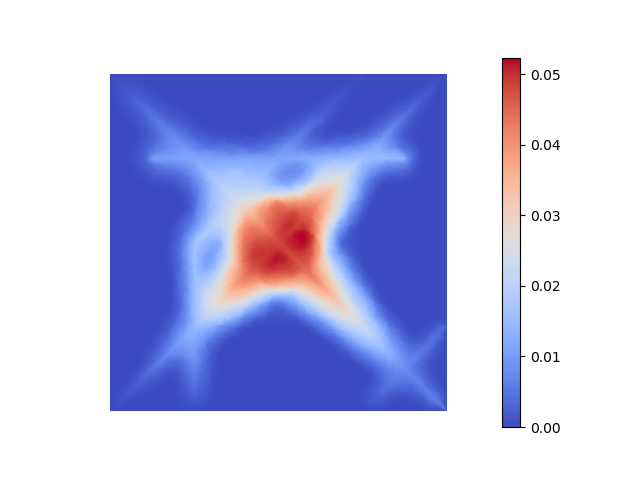
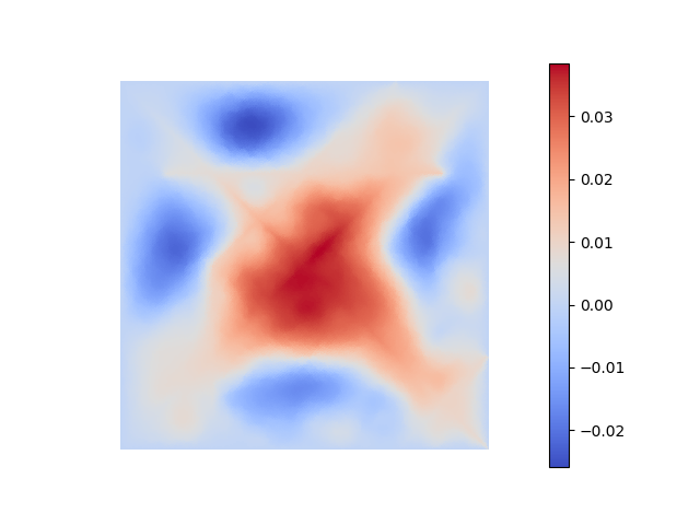
As an example, we consider the weak form (6) when the domain $\Omega$ is a unit square with an interface $\Gamma$ at $x=0.5,\ 0\leq y\leq 1$. The permeability on the interface is $A_{\Gamma}=5$, and the permeability $A$ in the bulk domain is piecewise constant with respect to a uniform Cartesian grid of width $2^{-7}$. The values are sampled from the uniform distribution in [0.1,0.9]. A triangulation $\mathcal{T}_{H}$ of $\Omega$ is constructed such that the interface $\Gamma$ is a union of coarse element edges, but $A$ is not well-resolved by $\mathcal{T}_{H}$. The fine space $V_{\mathrm{f}}$ is defined as the kernel of the Scott–Zhang interpolation operator [20], whose nodal variables on each node of $\mathcal{T}_{H}$ are computed by averaging the function in neighboring elements or edges.

Let $\lambda_{m}$ be the coarse basis function centered at $(0.5,0.5)$. First, we compute $Q\lambda_{m}$ by using the standard element-based Scott–Zhang interpolation operator. In this case, the integration domains are all elements connected to the corresponding node. We observe in Figure 3a that $Q\lambda_{m}$ decays slowly in the direction of the interface $\Gamma$. If we instead use an edge-based Scott–Zhang interpolation operator, we see fast decay shown in Figure 3b. Here, for the nodes on $\Gamma$, we only select neighboring edges that are also on $\Gamma$ as the integration domains; for all the other nodes, we integration domains are all neighboring elements. In Section 4, we give a proof for this case to justify that the decay is exponential. It turns out to be crucial to let nodal variables on and close to the interface to integrate only on the interface. This is in agreement with the observations in [10].

The above observation motivates a localization of (11) by restricting $\phi_{T}$ to a patch. For this we need the element neighbor operator $U(\omega)$ that maps the subdomain $\omega$ to a patch of elements that intersect with $\omega$ and define

When applied recursively, we get a multi-layer element neighbor operator $U^{k}(\omega)=U(U^{k-1}(\omega))$, where $k$ is the patch size. We use the convention $U^{1}(\omega):=U(\omega)$ and $U^{0}(\omega):=\omega$,. We also define $U_{\Gamma}(T)=U(T)\cap\Gamma$.

The restricted fine space ${\color[rgb]{0,0,0}V_{\mathrm{f}}(U^{k}(T))}\subset V_{\mathrm{f}}$ is defined as

We localize $\phi_{T}$ by defining $\phi_{T}^{k}\in{\color[rgb]{0,0,0}V_{\mathrm{f}}(U^{k}(T))}$ that satisfies

for all $w\in{\color[rgb]{0,0,0}V_{\mathrm{f}}(U^{k}(T))}$. The bilinear form $a_{k}(\cdot,\cdot)$ is defined on a patch of size $k$ as

and the values of $\phi_{T}^{k}$ outside the patch is zero. We have the best approximation property

We define the localized correction operator $Q_{k}$ as

for all $v\in V_{H}$. By applying the localized correction operator $Q_{k}$ to every basis function $\lambda_{i}$ of $V_{H}$, we obtain $\{Q_{k}\lambda_{i}-\lambda_{i}\}$ as a basis for the localized multiscale space $V_{\mathrm{ms}}^{k}$.

Given the space $V_{\mathrm{ms}}^{k}$ we are ready to present the localized version of the method. The LOD method then reads: find $u_{\mathrm{ms}}^{k}\in V_{\mathrm{ms}}^{k}$ such that

Since $V_{\mathrm{ms}}^{k}\subset V$, we have the Galerkin orthogonality

and the best approximation property

We have intentionally not discretized the restricted fine spaces $V_{\mathrm{f}}(U^{k}(T)),T\in\mathcal{T}_{H}$ at this stage to allow for different discretization methods to be used. In Section 6 we present the particular choice made in our numerical experiments. We choose a simple finite element discretization resolving the interfaces and the rapidly varying diffusion, see [4]. More sophisticated techniques as CutFEM [5] could be considered using a non-conforming LOD formulation similar to [8].

First, we consider the case when the fracture $\Gamma$ is a union of edges. Let $\mathcal{E}^{\Gamma}_{H}$ be the set of all closed element edges comprising $\Gamma$, i.e. $\Gamma=\bigcup\mathcal{E}^{\Gamma}_{H}$. We let $\mathcal{T}^{\Gamma}(N)=\{T\in\mathcal{T}(N)\,:\,N\in E\text{ and }E\subset T\text{ for some }E\in\mathcal{E}^{\Gamma}_{H}\}$, i.e. the adjacent triangles with at least one edge connected to the node also intersecting the fracture. With this choice, $\mathcal{N}^{\Gamma}$ contains the free nodes that intersect with $\Gamma$ and $\mathcal{N}^{\Omega}$ contains the remaining free nodes. See Figure 4 for illustrations of the resulting integration domains for a node in each set.

Before providing the proof that $\mathcal{I}_{H}$ satisfies Assumption 1 for this case, we make a few notes regarding the solution of (24). If $\Gamma$ is a union of coarse element edges, then $\sigma$ is either a coarse triangle or a union of coarse edges. If $\sigma$ is a coarse triangle, then (24) is a $(d+1)\times(d+1)$ linear system with the coarse basis mass matrix integrated over the coarse triangle. If $\sigma$ is a union of $n$ edges then (24) is a $(n+1)\times(n+1)$ linear system with the coarse basis mass matrix integrated over those edges.

Next, we consider the case when the fracture $\Gamma$ is not a union of edges in $\mathcal{T}_{H}$, but intersects with the interior of triangles. We will then pick integration domains $\sigma$ to be in the interior of the triangles as well. The shape of the integration domain influences the dual basis norm $\|\psi\|_{\sigma}$, which in turn influences the stability of the interpolation operator as a whole. For instance, the linear system (24) that determines $\psi$ will be rank deficient if $\sigma$ is a straight line in the intersection with the interior of $T$. For almost straight lines, the dual basis norm can become very large. In case the system is rank deficient but has infinitely many solutions, it is easy to see that any two solutions $\psi$ and $\psi^{\prime}$ have the same $L^{2}(\sigma)$-norm $\|\psi\|_{\sigma}=\|\psi^{\prime}\|_{\sigma}$. Infinite number of solutions arise, for example, when $\sigma$ intersects with the interior of $T$, is a straight line and passes through the node $N$. Next, we study an example where this norm is computed for two parametrized shapes of $\sigma$ that degenerate to straight lines as the parameter increases.

Because of this interplay between the mesh and the fracture geometry, we define $\mathcal{T}^{\Gamma}(N)$ to adaptively discard (by the means of an indicator) integration domains that give rise to large dual basis norms. We recall from [20] or [10, Lemma 3.4] how the dual basis for $(d-1)$-dimensional $\sigma$, the norm of $\psi$ scales with the triangle diameter as follows

where $\hat{\psi}$ is the solution to (24) in a transformed coordinate system such that $T$ is transformed to the simplex reference element $\hat{T}$ of diameter 1. When considering a node $N$, we define an indicator for all $T\in\mathcal{T}(N)$,

Given a threshold value $\Sigma$, we let

and use this $\mathcal{T}^{\Gamma}(N)$ to define $\mathcal{I}_{H}$ in (25). See Figure 6 for an illustration of how $\Sigma$ affects the choice of integration domain. For the previously discussed special case that the fracture is a union of edges, we obtain the same set as in Lemma 1 by $\mathcal{T}^{\Gamma}(N)=\{T\in\mathcal{T}(N)\,:\,s_{N,T}\text{ is finite}\}$.

We define the closure of the complement of $U^{k}(T)$ as $U^{k}_{c}(T):=\overline{\Omega\backslash U^{k}(T)}$. In the error analysis, we will frequently restrict functions to patches. It is helpful to consider a Lipschitz continuous cutoff function $\eta_{T}^{k}:\Omega\rightarrow[0,1]$ such that

and satisfies

An example of such a cutoff function is $\eta_{T}^{k}\in V_{H}$ with nodal values 0 in $U^{k}(T)$ and 1 in $U^{k+1}_{c}(T)$.

The following theorem states that the correctors decay exponentially fast away from the corresponding support.

References

• [1] Abdulle, A., Henning, P.: Localized orthogonal decomposition method for the wave equation with a continuum of scales. Math. Comp. 86, 549–587 (2017)
• [2] Alboin, C., Jaffré, J., Eoberts, J.E., Serres, C.: Modeling fractures as interfaces for flow and transport in porous media. Contemp. Math. 295, 13–24 (2002)
• [3] Angot, P., Boyer, F., Hubert, F.: Asymptotic and numerical modelling of flows in fractured porous media. ESAIM: Math. Model. Numer. Anal. 43, 239–275 (2009)
• [4] Burman, E., Hansbo, P., Larson, M.G.: A simple finite element method for elliptic bulk problems with embedded surfaces. Computat. Geosci. (2019)
• [5] Burman, E., Hansbo, P., Larson, M.G., Samvin, D.: A cut finite element method for elliptic bulk problems with embedded surfaces. Int. J. Geomath. 10 (2019)
• [6] Capatina, D., Luce, R., El-Otmany, H., Barrau, N.: Nitsche’s extended finite element method for a fracture model in porous media. Appl. Anal. 95, 2224–2242 (2016)
• [7] D’Angelo, C., Scotti, A.: A mixed finite element method for Darcy flow in fractured porous media with non-matching grids. ESAIM: Math. Model. Numer. Anal. 46, 465–489 (2012)
• [8] Elfverson, D., Georgoulis, E.H., Målqvist, A., Peterseim, D.: Convergence of a discontinuous Galerkin multiscale method. SIAM J. Numer. Anal. 51, 3351–3372 (2013)
• [9] Engwer, C., Henning, P., Målqvist, A., Peterseim, D.: Efficient implementation of the localized orthogonal decomposition method. Comput. Methods Appl. Mech. Eng. 350, 123–153 (2019)
• [10] Hellman, F., Målqvist, A.: Contrast independent localization of multiscale problems. Multiscale Model. Simul. 15, 1325–1355 (2017)
• [11] Hou, T.Y., Wu, X.: A multiscale finite element method for elliptic problems in composite materials and porous media. J. Comput. Phys. 134, 169–189 (1997)
• [12] Hughes, T.J.R., Feijóo, G.R., Mazzei, L., Quincy, J.: The variational multiscale method - paradigm for computational mechanics. Comput. Methods Appl. Mech. Eng. 166, 3–24 (1998)
• [13] Kornhuber, R., Peterseim, D., Yserentant, H.: An analysis of a class of variational multiscale methods based on subspace decomposition. Math. Comp. 87, 2765–2774 (2018)
• [14] Målqvist, A., Peterseim, D.: Localization of elliptic multiscale problems. Math. Comp. 83, 2583–2603 (2014)
• [15] Maier, R., Peterseim, D.: Explicit computational wave propagation in micro-heterogeneous media. BIT Numer. Math. 59, 443–462 (2019)
• [16] Martin, V., Jaffré, J., Roberts, J.E.: Modeling fractures and barriers as interfaces for flow in porous media. SIAM J. Sci. Comput. 26, 1667–1691 (2005)
• [17] Odsæter, L.H., Kvamsdal, T., Larson, M.G.: A simple embedded discrete fracture-matrix model for a coupled flow and transport problem in porous media. Comput. Methods Appl. Mech. Engrg. 343, 572–601 (2019)
• [18] Owhadi, H., Zhang, L., Berlyand, L.: Polyharmonic homogenization, rough polyharmonic splines and sparse super-localization. Esaim: Math. Model. Numer. Anal. 48, 517–552 (2014)
• [19] Peterseim, D., Scheichl, R.: Robust numerical upscaling of elliptic multiscale problems at high contrast. Comput. Meth. Appl. Mat. 16, 579–603 (2016)
• [20] Scott, L.R., Zhang, S.: Finite element interpolation of nonsmooth functions satisfying boundary conditions. Math. Comp. 54, 483–493 (1990)