Modeling Engagement Dynamics of Online Discussions using Relativistic Gravitational Theory
Abstract
Online discussions are valuable resources to study user behaviour on a diverse set of topics. Unlike previous studies which model a discussion in a static manner, in the present study, we model it as a time-varying process and solve two inter-related problems – predict which user groups will get engaged with an ongoing discussion, and forecast the growth rate of a discussion in terms of the number of comments. We propose RGNet (Relativistic Gravitational Network), a novel algorithm that uses Einstein Field Equations of gravity to model online discussions as ‘cloud of dust’ hovering over a user spacetime manifold, attracting users of different groups at different rates over time. We also propose GUVec, a global user embedding method for an online discussion, which is used by RGNet to predict temporal user engagement. RGNet leverages different textual and network-based features to learn the dust distribution for discussions.
We employ four baselines – first two using LSTM architecture, third one using Newtonian model of gravity, and fourth one using a logistic regression adopted from a previous work on engagement prediction. Experiments on Reddit dataset show that RGNet achieves Micro F1 score and average error for temporal engagement prediction of user groups and growth rate forecasting, respectively, outperforming all the baselines significantly. We further employ RGNet to predict non-temporal engagement – whether users will comment to a given post or not. RGNet achieves AUC for this task, outperforming existing baseline by AUC.
I Introduction
Emergence of social media has resulted in a large-scale, heterogeneous and dynamic space for the users to get engaged in different activities. Studying engagement patterns in such platforms has its own merit for multiple purposes: market researchers can identify their potential audience for advertising campaigns and lucrative strategies; political campaigners can develop wide-scale trend analysis of the mass on the effect of their propaganda, etc.
Engagement dynamics in social media has thus attracted wide attention over a decade. Past studies attempted to predict (i) which pair of users is more likely to get engaged with each other based on their history [1, 2], and (ii) which posts will engage more users [3, 4]. All these studies tackled the engagement prediction problem in a static manner by considering the entire discussion as a whole, thus ignoring dynamic user engagement and the micro-dynamics controlling temporal growth. The growth rate of a discussion, i.e., how many comments are being posted per unit time, varies over time, so as the user engagement. As the discussion continues, it unfolds diverse topics and user interactions, thus attracting different types of users over time. If we imagine users located in different points on a multidimensional space and clustered based on their coherent activities, a discussion can then be intuitively thought of as a growing and moving cloud in that space, attracting different sets of users in varying rates over time. The aim of the present work is to model the time-varying engagement dynamics of users with ongoing discussion – a completely novel problem without any previous work, to the best of our knowledge. We build a framework which jointly models two phenomena – user engagement from different clusters of users, and the rate of growth of discussions over time.
Different discussions attract different users at different rates. Although an individual user may get repelled by a particular discussion, the idea of repulsion cannot be consistently modeled without access to his/her cognitive data, or some platform-specific features such as dislike. This implies that the interaction between a user and a discussion is essentially attraction, which can be zero but always non-negative. This motivates us to imagine a discussion to induce a gravity-like force towards the users. In fact, if we rely on the relativistic definition of gravity (explained in Sec. III-A), it is even possible to adapt repulsion as a positive curvature in user manifold; however, in this work, we restrict ourselves to model interaction as ‘attraction’ only.
Newtonian model of gravitation describes gravity as a force following inverse squared distance law between particles – proportional to the mass of the particles and inversely proportional to their distance squared. Given two point particles of mass and placed at positions and respectively, the magnitude of the force of gravity between them, denoted by is given by,
| (1) |
where is the gravitational constant. In our hypothesis, discussions have some mass-like property which changes over time. Users ‘near’ to a discussion get attracted more. A ‘massive’ discussion tends to attract more users and therefore would achieve more growth rate. The degree of this ‘massiveness’ can be a function of the topic, relevance, properties of engaged users, etc. But Newtonian model does not explain how mass and distance (or spacetime, to be precise) interact with each other. In case of online discussions, users are not mere objects, rather they have histories, which bear complex connection with each other and the discussion itself.
In physics, cosmic phenomena such as motion of the Mercury around the Sun [5], bending of light passing near stars [6], etc. cannot be explained by Newtonian model of gravity. A more sophisticated understanding of gravitation, which explains the failure of Newtonian model, was given by Einstein with his ‘General Theory of Relativity’ [7] (GR Theory). Intuitively, relativistic theory of gravitation describes spacetime as an -dimensional Riemannian manifold, with dimensions for space and one dimension for time. Gravity is simply the curvature of this manifold at any point. According to this theory, the curvature can be caused by an object with mass and/or energy. Any object free-falling through this spacetime manifold must follow the ‘straightest’ path or geodesic – a path with constant directional derivative w.r.t. the manifold. More the mass/energy content of an object, more curved the spacetime will be around it, and hence more will be the effect of gravity. This ‘fusion’ of seemingly heterogeneous physical properties like mass/energy and spacetime by GR theory is the primary motivation behind our proposed model RGNet, which learns to efficiently fuse textual features of discussion with activity history of users in a temporal fashion to predict engagement dynamics.
Fig. 1 explains how we model engagement dynamics as a time-varying process (Table I summarizes important notations). In particular, our major contributions are five-fold:
- •
We propose GUVec, a novel algorithm to represent users of a discussion platform as fixed dimensional vectors based on their temporal, communicative and semantic proximity.
- •
We propose RGNet, an engagement prediction model which represents ongoing discussions as time-varying ‘dust clouds’ in the user manifold and models them using relativistic theory of gravity to predict which clusters of users from the manifold are likely to get engaged, and how fast the discussion cloud will grow.
- •
We propose two deep learning based models using Long Short-Term Memory (LSTM) cells, and a model similar to RGNet based on Newtonian model of gravity. We also adopt the work by Rowe and Alani [3] in temporal setting. All these models are considered as baselines.
- •
We also predict user engagement by adopting RGNet in a non-temporal setting (for the sake of a direct comparison with the existing baseline) – given a post, whether any user will comment to that post or not.
- •
We perform comprehensive evaluation on the Reddit CMV dataset [8] (for temporal engagement prediction) and Reddit r/news community (for non-temporal engagement prediction) to show the efficiency of GUVec and RGNet.
To the best of our knowledge, RGNet is the first model of its kind which is inspired by the fundamental theories of classical mechanics.
| Notation | Denotation |
|---|---|
| User co-occurrence matrix | |
| Metric tensor, inverse metric tensor | |
| Stress-energy tensor | |
| Ricci tensor, Ricci scalar | |
| Window size of comments | |
| No. of user clusters | |
| No. of windows in a discussion | |
| User set | |
| user cluster, set of cluster centers |
II GUVec: Global User Embedding
To compute user vectors from a discussion corpus, our proposed global user embedding method GUVec first constructs a user-user co-occurrence matrix . We use three different notions of proximity between two users and : (i) Communicative Proximity: they communicated with each other in a discussion; this happens when replied to in a discussion or vice versa, meaning they are present in the same chain of comments; (ii) Temporal Proximity: they are temporally close to each other; they are engaged in same discussion (have not replied to each other) nearly at the same time; (iii) Semantic Proximity: they are engaged in similar type of discussions.
To construct a meaningful embedding of users, we only take those who are engaged in at least two discussions. Given the entire set of such users denoted by , the co-occurrence matrix is symmetric and of dimension . To compute semantic proximity, we use ConceptNet Numberbatch word-vectors [9]. We take the words present in the discussion titles (after removing stopwords) and compute the weighted average of the corresponding word vectors. This weighted average now represents the title vector of discussion .
For any pair of users , their proximity is computed as follows:
- •
Communicative Proximity: If , replied to each other, then increment by 2.
- •
Temporal Proximity: If , commented on the same discussion at time and respectively, but did not reply to each other, then
(2) where and are the starting and ending times of the discussion, respectively.
- •
Semantic Proximity: If , commented on different discussions and , respectively, then
(3) where , and is a threshold angle (Sec. VI for parameter selection).
In Eq. 2, accounts for how much temporally close two comments are w.r.t. the total time span of the discussion. This normalizes temporal proximity of discussions growing in different rates. We put highest proximity value for two users if they replied to each other. Both the terms and have upper bound of . Therefore, for any pair of users, the contribution of their temporal and semantic proximity taken together cannot exceed their communicative proximity, which is incremented by 2.
Once is computed, GUVec minimizes the following objective function to obtain user vectors:
| (4) |
where and correspond to the user vector and bias, respectively. This objective function bears some similarity to that of GloVe embedding [10]. Eq. 4 uses the hypothesis that, for any two users and , the term should be proportional to the logarithm of the probability of occurring in the context of . This probability can be computed as , thus . Since , i.e., the probability of a user appearing in user ’s context is same as the reverse, we need to exclude the term containing . Hence we introduce the bias terms and in Eq. 4. We also need to assure that vectors of highly co-occurring users should be computed with greater accuracy. Therefore, we introduce the weighing term .
III RGNet: Modeling User Engagement
After computing user vectors, we group them into clusters using standard clustering methods (see Sec. VI). Henceforth, the cluster centers will represent -regions of user manifold. We will first explain the Einstein Field Equations and their components, followed by how RGNet incorporates them in modeling user engagement. Fig. 2 shows a schematic architecture of RGNet.
III-A Einstein Field Equations (EFE)
In general theory of relativity, spacetime is a four-dimensional manifold with one dimension of time and three dimensions of space. Gravity is not an external force (like electromagnetic or nuclear forces), rather an intrinsic property of spacetime, defined as curvature in . Any object without the effect of any force, will follow a geodesic (a curve for which directional co-variant derivative along the tangents of the curve remains zero) along this manifold. The geometry of the spacetime manifold is defined by sixteen Einstein Field Equations [7]:
| (5) |
This is a tensor equation, with , corresponding to dimension indices of the spacetime. As there are total four dimensions (one for time and three for space), the pair can take sixteen different values. , and are three constants – Newtonian gravitational constant, cosmological constant and velocity of light in vacuum, respectively. is called the metric tensor of the manifold. This is a contra-variant tensor which gives the idea of distance between two vectors on a manifold:
| (6) |
where is the difference in the component of two vectors. It has its covariant counterpart , which is called the inverse metric.
is the Ricci curvature tensor. is the corresponding Ricci scalar. The change in a vector for parallel transport (i.e., following a geodesic) along two different infinitesimal flows in a smooth manifold is given by the Riemann Curvature tensor. Ricci tensor is the contraction of Riemann tensor on the second index. Both Ricci and Riemann tensors can be computed from second order derivatives of the metric tensor. We define Christoffel symbol of second kind as ,
| (7) |
where is the partial derivative of with respect to the component. Then, is defined as,
| (8) |
Eqs. 7 and 8 are seemingly very complex to directly compute using metric tensor. However, the important fact is that Ricci tensor can be computed as a function of derivatives of the metric tensor, and therefore, as differential function of the components of points in the manifold. Ricci scalar is simply the trace of the Ricci tensor:
Intuitively, in a 2D manifold, a zero Ricci scalar at a point indicates that the manifold is flat at that point; negative value indicates a saddle point, and positive value indicates a hill. In Eq. 5, the term describes the curvature of the spacetime manifold at any point. Its trace with respect to the inverse metric yields negative scalar curvature:
| (9) |
is called the stress-energy tensor. For an infinitesimal volume of spacetime manifold, its components represent the properties as shown in Fig. 3. For an isolated massive particle, all the components except are zero. For a cloud of dust, only the diagonal elements have non-zero value.
Multiplying both sides of Eq. 5 by inverse metric tensor yields,
| (10) |
III-B EFE in Discussion Spacetime
Eq. 5 does not have any static solution without the cosmological constant , indicating the universe is expanding. Einstein introduced to make it static, which, upon the observation of expanding universe in reality by Hubble [11], was discarded later. In our particular case of learning engagement dynamics in discussions using general relativity, we also omit and reduce the constants in Eq. 10 to yield
| (11) |
where represents the position of user cluster in the user manifold we computed in Sec. II, is the set of features representing the discussion, is the dimension of the user vectors, is the inverse metric tensor which is computed as a function of cluster positions, is the stress-energy tensor counterpart for discussion which is computed as a function of cluster positions and features of discussion. We prepend the time value to each user vector to convert it into a -dimensional spacetime manifold. RGNet learns each component of Eq. 11 as a series of non-linear transformations: , where and are input and output of the transformation respectively, is a bounded non-linear function, and are weight and bias matrices to be learned respectively.
It is important to note that relativistic model of spacetime requires multiple constraints to be fulfilled. First of all, physical laws should be observer independent – one can choose any frame of reference (rotated, translated, moving w.r.t. another frame of reference) and the physics must remain the same. General Relativity requires this constraint to be local. The user manifold obtained from GUVec computes the position of a user in the manifold using the vector dot product, which is invariant to rotation and translation. Moreover, it takes into account the temporal proximity of two users. We expect this to reflect invariance to temporal transformations of the manifold as well. However, engagement over online discussions is not a deterministic physical process. We claim it to be only analogous to spacetime geometry and not an exact replica. So in our case, Einstein’s Field Equations are only abstract approximation learnt by RGNet. An exact mathematical model of engagement is far more complex, if not intractable.
We define the temporal progress of a discussion as windows of comments of fixed size . This means, at the step, the size of our discussion is (post + comments), and we need to predict for the next comments. Due to variable size of discussions, we define maximum size of the discussion to be , where is the number of windows, and hence, the number of prediction steps for a single discussion. All the discussions with size less than the maximum size are zero-padded at the end.
III-C Feature Selection
For the original post and every comment in the discussion, we extract following features based on the content, user, surface structure of the text.
(i) Content Features:
Average of tf-idf scores of the tokens. This represents how many unique and relevant words are used in the comment.
LIX readability score [12], computed as:
,
where and are the sets of words and sentences respectively, and is the set of words with more than six characters. Larger the value of , harder the comment/post is to read in a short time.
Cumulative entropy of terms, given by ,
where is the set of all unique tokens in the corpus, and is the frequency of term in the comment/post.
Polarity of the comment/post, i.e., sum of sentiment intensity scores of the unique terms computed using SenticNet [13]. We also use the total number of positive and negative sentiment words as polarity features.
(ii) Surface Features: We use the following surface features – total number of sentences in the text, average number of words per sentences, count of URLs present in the comment, depth of the comment in discussion tree, time difference of the comment with the post and the count of closing punctuation markers, i.e., ‘.’,‘!’ and ‘?’ (as different types of closing punctuation markers signify different discourse).
(iii) Latent Semantics: We use the pre-trained word vectors mentioned in Sec. II to represent the latent semantics of the text. Every comment is represented as a vector: ), where is the set of unique terms in the comment, and is the word vector of term. For the post, we also use the title vectors mentioned in Sec. II as features.
(iv) User Features: We use user vectors computed by GUVec as user-based features, which reflect past activity and connections of a user.
For a total number of features representing each comment, the representation of a post is then an array of size with being the size of word vectors used; all the comments taken together is an array of size , and user manifold regions are represented as an array of size for a single discussion.
III-D Stress-Energy Tensor of Discussion
First, we compute an intermediate representation of the post and the comments with dimension:
| (12) |
now contains representation of the post and each of the comment windows. and (where ) mentioned throughout the paper indicate the learnable weight and bias matrices, respectively. is the rectified linear unit function. Now all the representations from 0 to steps should contribute at step. Therefore, we take a weighted cumulative sum of :
| (13) |
Next, we concatenate to each and compute the corresponding stress-energy tensor:
| (14) |
where . Each is a -dimensional vector representing the diagonal elements of the stress-energy tensor of Eq. 11.
III-E Inverse Metric Tensor
We compute the values of inverse metric tensor for prediction step at cluster region as a function of the cluster center as follows:
| (15) |
Again, this is a -dimensional vector which represents the diagonal of the inverse metric tensor of Eq. 11.
III-F Curvatures of Manifold
Once we obtain the stress-energy tensor and the inverse matrix tensor of the discussion at prediction step for cluster, we compute the scalar curvature of the manifold at cluster based on Eq. 11 as,
| (16) |
This step actually performs the fusion of textual and user interaction features. The extent to which the discussion attracts users towards it for the entire manifold can be computed as the weighted sum of each of , given by,
| (17) |
Finally, we define cluster engagement probability and discussion growth velocity as two nonlinear functions of cluster-wise scalar curvature and total curvature respectively:
| (18) |
so that and , befitting to both user cluster engagement prediction and growth rate forecasting tasks. Altogether, we train RGNet to learn the following function:
| (19) |
For user cluster engagement prediction task (multi-label classification), we use binary cross-entropy loss with as the threshold, and for the growth rate forecasting (regression), we use mean squared error loss to train RGNet.
IV Baselines for Temporal Engagement
Due to the lack of existing baseline in predicting temporal user engagement, we design four baselines:
(i) Newtonian Model: This model is similar to RGNet except it uses Newtonian model over flat space instead of spacetime manifold. We compute based on Eqs. 12 and 13 using same set of features, except instead of computing a stress-energy tensor for each cluster (Eq. 14), we compute a scalar mass at the prediction step:
| (20) |
We compute the position of the discussion at prediction step on the -dimensional space as a weighted average of user vectors commented till prediction,
| (21) |
(ii) LSTM Models: We implement two LSTM models; one with the features we defined in Sec. III-C (LSTM-f), another using raw text data (LSTM-r). To input raw text data, we use one-hot encoding of each word and initialize an embedding layer with pre-trained word vectors mentioned in Sec. II. This model uses an extra layer of LSTM cells to compute the representation of comments from words. Both these models use same loss functions (binary cross-entrpoy and mean squared error). Fig. 4 shows the architecture.
(iii) Logistic Regression: Lastly, we implement a logistic regression classifier adapted from the model proposed by Rowe and Alani [3]. We consider the same set of features except the duration of a user in the community as Reddit does not provide this data. The authors broadly categorized the features used as social and content features. Their original work is not designed for temporal engagement modeling. Also, they performed a binary classification of whether a post will get commented or not. We adopt this model for our task with two modifications: (a) we take each user cluster and predict whether a user from this cluster will comment (user-network based features are calculated for each cluster separately, not the whole user-user interaction network) and (b) at each prediction step for a particular discussion, we take the post and comments (if any) till that instance as a single entity – content features are calculated from the merged texts of post and comments, and the average of social features of the users who posted/commented is considered as the cumulative social feature. This model is made only for predicting engagement of user clusters.
V Non-temporal Engagement Prediction
As already stated, our defined problem of predicting temporal engagement dynamics is novel, and there is no existing work which can be directly considered to compare with RGNet. Rowe and Alani [3] (henceforth, referred as R&A) proposed a framework to predict engagement in a non-temporal manner. Given a post, their model predicts whether it will attract any user or not. We modify RGNet to suit this task and compare the performance.
We hypothesize that, if a post fails to curve the user manifold ‘effectively’, it will not attract any users in the future. For this, we input the post feature to RGNet. As this is a one-shot prediction for the post only, the comment feature as well as the comment window are irrelevant here. Also, all the occurrences of in the governing equations of RGNet have a single value (i.e., ), as this is the first prediction step in the full implementation of RGNet. Therefore, the stress-energy tensor in Eq. 14 is computed from only (first part of Eq. 12). Total curvature (in Eq. 17) estimates the degree of total attraction generated by the post. We compute the probability of a post to attract any user at all from the total curvature as:
| (23) |
Here, ranges in interval . We take as negative class (post fails to attract any user), and positive class, otherwise.
VI Experimental Setup
We describe the datasets and parameter selection for RGNet: both for temporal and non-temporal engagement prediction.
VI-A Datasets
The Reddit CMV dataset that we used contains discussions from Jan 1, 2013 - May 7, 2015 for training, and discussions from May 8, 2015 - Sep 1, 2015 for testing. We excluded comments posted by deleted users and delta-bots (carrying author-tags “deleted” and “DeltaBot” respectively) and users who commented only once. This leaves our training (test) set with () users and () comments in total.
However, this CMV dataset was originally filtered, such that there is no post which failed to attract any user comment. Therefore, we cannot use this dataset for non-temporal engagement prediction. For this task, we crawled posts from Reddit news community. We collected a total of posts from Sep 1, 2016 to Jan 16, 2019, out of which posts do not have any comments. To avoid classification bias, we take equal number of posts containing comments. Here again, we excluded users who have commented/posted only once or carry the author tag “deleted” (delta-bots does not appear in this community) to compute the GUVec embeddings. This results in a total of users.
VI-B Parameter Selection
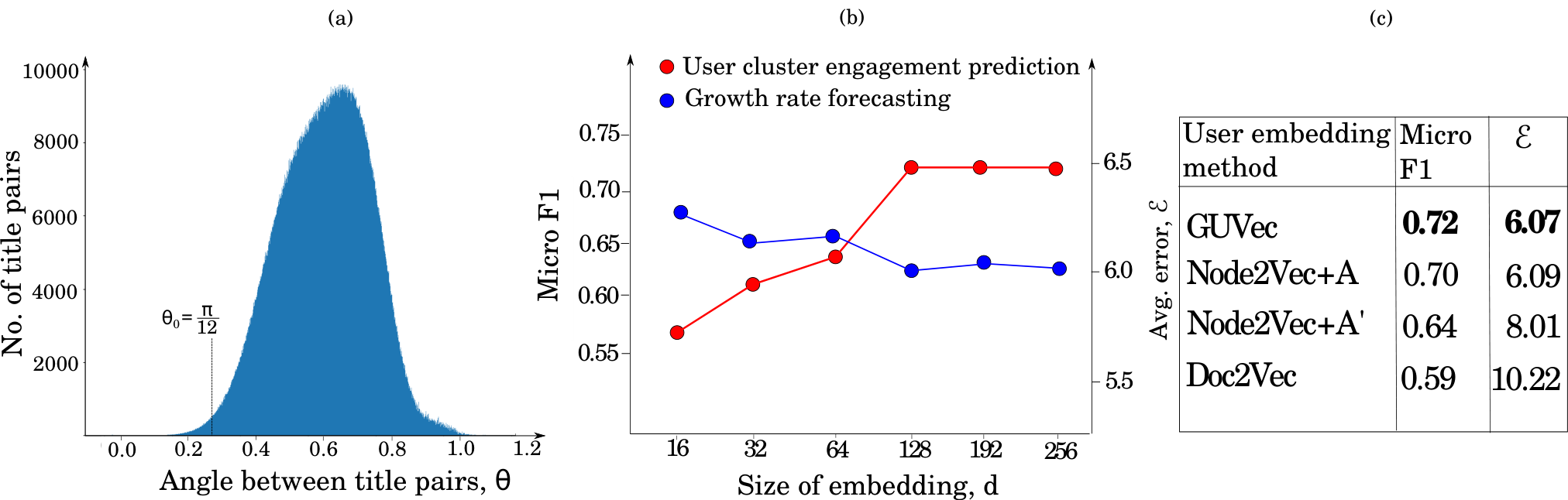
While constructing the co-occurrence matrix , computing the semantic proximity is computationally the most expensive part as we need to count for all possible pairs of users between every pair of discussions. The choice of in Eq. 3 can significantly reduce this cost if we pre-compute between pairs of discussion titles and take into account only those discussions having . In Fig. 5(a), we plot the number of discussion title pairs with between them. Discussion pairs with amounts to of the total pairs. We find that the number of user-pairs for this subset is . Therefore we choose to be .
We vary the embedding dimension from 16 to 256. Fig. 5(b) shows that the performance of RGNet does not change much after . We cluster user embedding space using K-means by varying K from , , to .11 1 We also tried with agglomerative and DBSCAN methods for user clustering and observed similar results. In case of engagement modeling, we vary window size from to . All the models except the logistic regression were optimized using Adam [14] optimization algorithm. Unless otherwise stated, we use the following parameter values as default: , , , and .
| Metric | Description | Formula |
|---|---|---|
| Micro F1 | Micro average of precision and recall on all binary labels | |
| Macro F1 | Macro average of precision and recall | |
| Hamming Loss | Average error rate over all the binary labels | |
| Subset Loss | Average % when predicted label set is exactly correct |
VII Experimental Results
We perform comparative evaluation for three tasks separately. For temporal engagement dynamics, we compare RGNet with other baselines to predict user cluster engagement and growth rate forecasting. For non-temporal engagement, we present the performance of RGNet for different number of clusters and compare it with R&A [3]. We study the importance of different features for these tasks. We also show the efficiency of GUVec compared to other embedding methods for temporal engagement tasks mentioned above, and empirically show the complexity of GUVec. In the end, we present a case study of user cluster engagement prediction obtained from RGNet.
| Method | HL | MiF | MaF | 0/1 |
|---|---|---|---|---|
| RGNet | 0.27 | 0.72 | 0.65 | 0.78 |
| LSTM-f | 0.36 | 0.64 | 0.57 | 0.81 |
| LSTM-r | 0.37 | 0.61 | 0.56 | 0.81 |
| Newton. | 0.40 | 0.56 | 0.51 | 0.86 |
| Logistic Regression | 0.36 | 0.62 | 0.56 | 0.85 |
VII-A Predicting Temporal Engagement of User Clusters
We pose user cluster engagement prediction problem as a multi-label classification problem. At prediction step, let there be comments in the window, with . Let there be clusters of the user manifold. Each instance in our dataset corresponds to a window. For window, we create the ground-truth binary vector of size such that, if there is at least one comment in the window from a user belonging to cluster, otherwise.
Table III reports the performance of the competing methods based on four standard metrics used for multi-label classification [15] (see Table II for the description) – Hamming Loss (HL), Micro F1 (MiF), Macro F1 (MaF), and Subset 0/1 (0/1). RGNet outperforms others across all the metrics – it beats the best baseline (LSTM-f) by 12.5% (14.03%) higher Micro (Macro) F1 .
Table IV(a) shows that as the number of clusters grows, the average degradation of performance for RGNet and Newtonian model is minimum (15.22% and 10.15% respectively averaged across consecutive values of ) compared to others (15.14% for LSTM-f). These two models benefit from the fact that, with smaller cluster size, cluster centers exhibit accurate locality of the cluster, which helps them compute more accurate curvature and the distance vector. Table IV(b) shows that for most of the models, the performance increases as the window size grows.
To check how homogeneity of users (in terms of their clusters) already engaged till window affects the performance for window, we compute the entropy of the cluster membership of users engaged till window, as , where is the fraction of users in belonging to cluster . Fig. 6(a) indicates that as increases (users already engaged tend to be members of same cluster), the performance decreases (Pearson ) since the model tends to predict more to the cluster whose members are engaged more in discussion. This further results more mistakes for those clusters which have not been engaged so far in the discussion. However, the decrease in performance is less for RGNet compared to the best baseline.
| Model | (a) # of clusters, (Micro F1, ) | |||
|---|---|---|---|---|
| 8 | 16 | 24 | 32 | |
| RGNet | 0.72,11.02 | 0.62,7.93 | 0.53,6.54 | 0.44, 6.01 |
| LSTM-f | 0.64,11.23 | 0.57,10.87 | 0.46,9.92 | 0.39,10.56 |
| LSTM-r | 0.61,21.55 | 0.53,19.12 | 0.46,20.04 | 0.38,21.87 |
| Newt. | 0.56,24.66 | 0.48,28.54 | 0.42,25.01 | 0.40,23.12 |
| Model | (b) Window size, (Micro F1, ) | |||
|---|---|---|---|---|
| 5 | 10 | 15 | 20 | |
| RGNet | 0.54,8.04 | 0.66,6.07 | 0.72,6.01 | 0.69,6.12 |
| LSTM-f | 0.49,12.56 | 0.55,11.20 | 0.64,11.23 | 0.65,10.98 |
| LSTM-r | 0.49,24.32 | 0.54,22.87 | 0.61,21.55 | 0.61,21.45 |
| Newt. | 0.32,29.57 | 0.46,27.01 | 0.56,24.66 | 0.57,25.03 |
VII-B Growth Rate Forecasting for Temporal Engagement
We define the growth rate of engagement for a discussion at window as , where is the time difference of first and last comments in window, and is the window size. To test how effectively each competing model predicts the growth rate for window, we use relative %-error in prediction given by , where () is the actual (predicted) value. Table IV(a) shows the average error across all the windows incurred by the models trained with different number of clusters . We observe that as increases, the average error for RGNet decreases. The reason is that more the number of clusters obtained from user embedding, more precisely RGNet can compute the curvature throughout the manifold.
Fig. 6(b) shows the correlation of per-window error and true growth rate (for better visualization, we normalize by its maximum value obtained). We observe that for higher values of growth rate, prediction is more erroneous (Pearson ). We empirically observe that such a large growth rate occurs when more that comments appear per second. Such instances (discussions) seldom appear in our dataset (1.74% of total discussions).
VII-C Non-temporal Engagement Prediction
| Model | F1-score | AUC | Accuracy |
|---|---|---|---|
| RGNet-8 | 0.51 | 0.52 | 0.52 |
| RGNet-16 | 0.54 | 0.55 | 0.57 |
| RGNet-24 | 0.61 | 0.62 | 0.63 |
| RGNet-32 | 0.59 | 0.59 | 0.60 |
| R&A | 0.56 | 0.57 | 0.58 |
In Table V, we present the performances of different models for predicting whether a given post will attract users or not. We observe that RGNet with 24 clustering of the manifold performs the best. Moreover, both settings with 24 and 32 clusters outperform R&A by a significant margin.
In Table V, we can observe an increase in performance of RGNet for this task as the number of clusters grows. A possible reason might be the heterogeneous distribution of users over the manifold and how accurately RGNet is being informed about this heterogeneity. It is already explained that more closely located users (i.e., users in a dense cluster) are more likely to interact with each other in near future. Therefore, a post coming from an outlier user is less likely to be replied by other users. With less number of clusters, sparsely separated users are identified to be members of a cluster. This results in RGNet assigning wrong curvature value for those users. With more clusters, this error is minimized. However, with increasing number of clusters, errors in curvature computation for each cluster get accumulated and affect the total curvature . This possibly explains the performance drop for RGNet with clusters in Table V.
VII-D Feature Importance
We perform feature ablation study for both temporal and non-temporal engagement prediction tasks. For the former case, we study feature importance only for RGNet, whereas for the latter case, the analysis is done for both RGNet and R&A.
VII-D1 Feature Ablation for Temporal Engagement
We study the importance of different features for RGNet in two settings. In the first setting, we drop each group of features (mentioned in Sec. III-C) in isolation and report the accuracy. In the second setting, we add random noise to each feature in isolation – we draw random samples from Gaussian distributions with same mean and standard deviation as that of the original distribution of the feature (this experiment was repeated 10 times, and the average result was reported). Table VI indicates that user features bear utmost importance for both the tasks, though its effect is more visible in user cluster engagement prediction than the growth rate prediction. This is quite consistent with our intuition that similar types of users tend to flock together.
| Feature set |
|
| ||||
|---|---|---|---|---|---|---|
| Micro F1 | Micro F1 | |||||
| Latent | 0.62 | 8.33 | 0.57 | 16.56 | ||
| User | 0.54 | 8.34 | 0.52 | 17.15 | ||
| Content | 0.59 | 7.12 | 0.56 | 15.42 | ||
| Surface | 0.63 | 8.43 | 0.57 | 14.89 | ||
| Model | Features used | F1-score |
|---|---|---|
| RGNet-24 | Content | 0.55 |
| Social | 0.58 | |
| R&A | Content | 0.52 |
| Social | 0.55 |
VII-D2 Feature Ablation for Non-temporal Engagement
For the non-temporal engagement prediction task, we perform feature ablation study for both RGNet and R&A. Rowe and Alani [3] grouped the features into two categories – content features and social features. Content features of R&A are closely similar to content, surface and latent features of RGNet (see Sec. III-C), with many features common in both the models. We group these features as content features as a whole in this study, and name the user features as social features, for a better comparison between these two models. We use the best performing version of our model (RGNet-24) for the feature importance study. Table VII shows that both the models treat social features with higher importance compared to content features for this task.
VII-E Performance of GUVec
We compare GUVec with three baselines: Node2Vec [16] is run on (i) our co-occurrence matrix (Node2Vec+) and (ii) a user-user matrix , where indicates the number of discussions where users and participated together (Node2Vec+); third baseline is designed by aggregating all the comments/posts by user in the training set and running Doc2Vec [17] on the aggregated text to obtain user embedding (Doc2Vec)22 2 The results of Node2Vec and Doc2Vec were reported after appropriate parameter tuning.. Fig. 5(c) shows that GUVec performs the best in both the tasks.
We also present an empirical study on the complexity of GUVec. Intuitively, building the user-user co-occurrence matrix is computationally most expensive, as it needs pair-wise comparison between users. Any pair-wise computation from an input of size results in an worst case time complexity of . As we compute the full matrix, this bound should be same for space complexity, too. However, GUVec does not take pairs from the full user set but only a finite subset . Complexity of building is readily reflected by the number of non-zero elements in , because only these elements correspond to a pair-wise comparison between users.
In Fig. 7, we plot the number of non-zero elements in the co-occurrence matrix with varying sizes of user sets. For a comparative understanding, we also plot the curves of , and . As we can see, the complexity of GUVec falls in between and . This is due to high clustering of users in the user-user interaction network; users tend to form groups and their interactions remain mostly within the group. For this, GUVec needs to compute pair-wise proximity values for pairs from very small subsets of . Let us assume that the user set is fragmented into equal-size partitions. Then, the total number of pair-wise computations GUVec needs will be . From Fig. 7, we know that, , which further simplifies to bounds of itself, given by, .
VII-F Diagnostics with a Case Study
Fig. 8 presents an example of the user cluster engagement prediction results by RGNet for first three consecutive windows. We observe that RGNet always computes high curvature for the cluster containing the users who started the discussion. It thus leads to an erroneous prediction for window, where RGNet predicts that users from cluster- will be engaged. Even in the window, a high curvature value is assigned to this cluster (darkest shade compared to rest of the clusters). Moreover, clusters from which users have been engaged in a window, tend to hold a high curvature value in the successive steps (cluster-, for example). It is important to note that these are absolute values of curvature; originally, more attraction means more negative curvature.
For every window, RGNet computes for each cluster center. Using Eq. 6, we then compute intra-cluster distance for each cluster at every window. Table VIII shows that metric distance (distance between two vectors computed using Eq. 6) is always greater than flat Euclidean distance; more the curvature for a cluster (hence more probable the users from that cluster are to get engaged), more is the stretching of the intra-cluster distance.
VIII Related Work
Various social media platforms enable users with different types of activities. In case of Twitter, a large body of literature address the problem of retweet prediction and user influence detection [18, 19]. Liu et al. [20] proposed a user behavior model for retweet prediction. Recently, studies on the role of multimodality in retweet prediction have gained much focus [21, 22]. Another problem, which is much similar to ours, is the reply prediction [23, 2, 1, 3]. For both the tasks, various sets of features were employed, which can be broadly categorized into two groups – content features and social features. As Cha et al. [24] and Macskassy and Michelson [25] suggested, content features play a vital role in retweet prediction; whereas replies are more dominated by social features [26, 1]. Reply networks were studied in various other platforms: Boards.ie, SAP community network33 3 https://www.sap.com/index.html, Facebook and many others [3]. Most of these studies predict which post is going to get more replies, typically ignoring the temporal dynamics of discussions. Other studies explored the evolving structural properties of reply network [27, 28, 29]. Purohit et al. [30] proposed a framework to predict user engagement in clusters formed from topic-based discussions over Twitter.
| Cluster ID | ED | MD-0 | MD-1 | MD-2 |
|---|---|---|---|---|
| 1 | 0.259 | 0.318 | 0.323 | 0.298 |
| 2 | 0.179 | 0.222 | 0.226 | 0.239 |
| 3 | 0.210 | 0.254 | 0.247 | 0.245 |
| 4 | 0.286 | 0.298 | 0.301 | 0.311 |
| 5 | 0.232 | 0.261 | 0.275 | 0.279 |
| 6 | 0.175 | 0.185 | 0.181 | 0.192 |
| 7 | 0.198 | 0.220 | 0.223 | 0.267 |
| 8 | 0.205 | 0.237 | 0.229 | 0.229 |
IX Conclusion
In this work, we adopted General Theory of Relativity to devise efficient fusion of heterogeneous features for modeling temporal and non-temporal dynamics of user engagement in online discussions. Our contributions in this work are: (i) GUVec, a novel user embedding method to represent users in a discussion platform as distributed vectors based on three different notions of proximity, (ii) RGNet, a novel user engagement model inspired by Einstein Field Equations, (iii) a comprehensive set of features characterizing a discussion (post, comments, and users), and (iv) an exhaustive comparative analysis to show the superior performance of RGNet compared to other baselines for temporal and non-temporal user engagement prediction and growth rate forecasting.
References
- [1] J. Schantl, R. Kaiser, C. Wagner, and M. Strohmaier, “The utility of social and topical factors in anticipating repliers in twitter conversations,” in ACM WebSci. ACM, 2013, pp. 376–385.
- [2] N. J. Yuan, Y. Zhong, F. Zhang, X. Xie, C.-Y. Lin, and Y. Rui, “Who will reply to/retweet this tweet?: The dynamics of intimacy from online social interactions,” in WSDM. ACM, 2016, pp. 3–12.
- [3] M. Rowe and H. Alani, “Mining and comparing engagement dynamics across multiple social media platforms,” in ACM WebSci. ACM, 2014, pp. 229–238.
- [4] V. Noguti, “Post language and user engagement in online content communities,” European Journal of Marketing, vol. 50, no. 5/6, pp. 695–723, 2016.
- [5] U. Le Verrier, “Lettre de m, le verrier à m: Faye sur la théorie de mercure et sur le mouvement du périhélie de cette planète,” Comptes rendus hebdomadaires des séances de l’Académie des sciences, vol. 49, pp. 379–383, 1859.
- [6] J. Soldner, “On the deflection of a light ray from its rectilinear motion, by the attraction of a celestial body at which it nearly passes by,” Berliner Astronomisches Jahrbuch, pp. 161–172, 1804.
- [7] A. Einstein, “Die feldgleichungen der gravitation,” Sitzung der physikalische-mathematischen Klasse, vol. 25, pp. 844–847, 1915.
- [8] C. Tan, V. Niculae, C. Danescu-Niculescu-Mizil, and L. Lee, “Winning arguments: Interaction dynamics and persuasion strategies in good-faith online discussions,” in WWW, 2016, pp. 613–624.
- [9] R. Speer and J. Chin, “An ensemble method to produce high-quality word embeddings,” arXiv preprint arXiv:1604.01692, 2016.
- [10] J. Pennington, R. Socher, and C. Manning, “Glove: Global vectors for word representation,” in EMNLP, 2014, pp. 1532–1543.
- [11] E. Hubble, “A relation between distance and radial velocity among extra-galactic nebulae,” PNAS, vol. 15, no. 3, pp. 168–173, 1929.
- [12] C.-H. Björnsson, “Readability of newspapers in 11 languages,” Reading Research Quarterly, pp. 480–497, 1983.
- [13] E. Cambria, S. Poria, D. Hazarika, and K. Kwok, “Senticnet 5: Discovering conceptual primitives for sentiment analysis by means of context embeddings,” in AAAI, 2018, pp. 1795–1802.
- [14] D. P. Kingma and J. Ba, “Adam: A method for stochastic optimization,” arXiv preprint arXiv:1412.6980, 2014.
- [15] C. Shi, X. Kong, D. Fu, P. S. Yu, and B. Wu, “Multi-label classification based on multi-objective optimization,” ACM TIST, vol. 5, no. 2, pp. 35:1–35:22, Apr. 2014.
- [16] A. Grover and J. Leskovec, “Node2vec: Scalable feature learning for networks,” in SIGKDD, 2016, pp. 855–864.
- [17] Q. Le and T. Mikolov, “Distributed representations of sentences and documents,” in ICML, 2014, pp. 1188–1196.
- [18] Q. Zhang, Y. Gong, J. Wu, H. Huang, and X. Huang, “Retweet prediction with attention-based deep neural network,” in CIKM, 2016, pp. 75–84.
- [19] J. Cheng, L. Adamic, P. A. Dow, J. M. Kleinberg, and J. Leskovec, “Can cascades be predicted?” in WWW. ACM, 2014, pp. 925–936.
- [20] Y. Liu, J. Zhao, and Y. Xiao, “C-rbfnn: A user retweet behavior prediction method for hotspot topics based on improved rbf neural network,” Neurocomputing, vol. 275, pp. 733–746, 2018.
- [21] K. Wang, M. Bansal, and J.-M. Frahm, “Retweet wars: Tweet popularity prediction via dynamic multimodal regression,” in WACV. IEEE, 2018, pp. 1842–1851.
- [22] Z. Zhao, L. Meng, J. Xiao, M. Yang, F. Wu, D. Cai, X. He, and Y. Zhuang, “Attentional image retweet modeling via multi-faceted ranking network learning.” in IJCAI, 2018, pp. 3184–3190.
- [23] R. Nishi, T. Takaguchi, K. Oka, T. Maehara, M. Toyoda, K.-i. Kawarabayashi, and N. Masuda, “Reply trees in twitter: data analysis and branching process models,” Social Network Analysis and Mining, vol. 6, no. 1, pp. 1–13, 2016.
- [24] M. Cha, H. Haddadi, F. Benevenuto, and K. P. Gummadi, “Measuring user influence in twitter: The million follower fallacy,” in ICWSM, 2010, pp. 10–17.
- [25] S. A. Macskassy and M. Michelson, “Why do people retweet? anti-homophily wins the day!” in ICWSM, 2011, pp. 209–216.
- [26] D. Sousa, L. Sarmento, and E. Mendes Rodrigues, “Characterization of the twitter@ replies network: are user ties social or topical?” in Proceedings of the 2nd international workshop on Search and mining user-generated contents. ACM, 2010, pp. 63–70.
- [27] E. Bakshy, J. M. Hofman, W. A. Mason, and D. J. Watts, “Everyone’s an influencer: quantifying influence on twitter,” in WSDM. ACM, 2011, pp. 65–74.
- [28] R. A. Baños, J. Borge-Holthoefer, and Y. Moreno, “The role of hidden influentials in the diffusion of online information cascades,” EPJ Data Science, vol. 2, no. 1, pp. 1–16, 2013.
- [29] P. Cogan, M. Andrews, M. Bradonjic, W. S. Kennedy, A. Sala, and G. Tucci, “Reconstruction and analysis of twitter conversation graphs,” in Proceedings of the First ACM International Workshop on Hot Topics on Interdisciplinary Social Networks Research. ACM, 2012, pp. 25–31.
- [30] H. Purohit, Y. Ruan, A. Joshi, S. Parthasarathy, and A. Sheth, “Understanding user-community engagement by multi-faceted features: A case study on twitter,” in WWW 2011 Workshop on Social Media Engagement (SoME), 2011.
- [31] L. Zhu, D. Guo, J. Yin, G. Ver Steeg, and A. Galstyan, “Scalable temporal latent space inference for link prediction in dynamic social networks,” IEEE TKDE, vol. 28, no. 10, pp. 2765–2777, 2016.
- [32] J. He, M. Ostendorf, X. He, J. Chen, J. Gao, L. Li, and L. Deng, “Deep reinforcement learning with a combinatorial action space for predicting popular reddit threads,” arXiv preprint arXiv:1606.03667, 2016.
- [33] B. D. Horne, S. Adali, and S. Sikdar, “Identifying the social signals that drive online discussions: A case study of reddit communities,” in ICCCN. IEEE, 2017, pp. 1–9.