An energy stable $C^{0}$ finite element scheme for a quasi-incompressible phase-field model of moving contact line with variable density

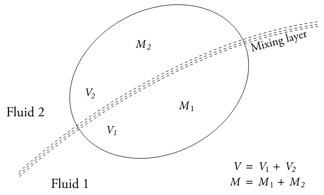
We consider a complex mixture consisting of two phase fluids with different densities. The interface of two fluids intersects with the wall $\partial\Omega_{w}$ at the contact line $\Gamma_{w}$ (see Fig. 1 (a)). Around the interface, we choose a control volume $V(t)$, where there are two phases labeled by $i=1,2$ with volume $V_{i}$ and mass $M_{i}$ (see Fig. 1 (b)). If the local average density of each phase is denoted by $\bar{\rho}_{i}=M_{i}/V$ and pure phase density is denoted by $\rho_{i}=M_{i}/V_{i}$, then density of mixture is

Let $c_{i}=\frac{M_{i}}{M}$ be the mass fraction of each phase. Then we have [62]

where $c=c_{1}$ is adopted in the last equality.

If we assume those two fluids move with velocities $\mathbf{u}_{i}$ ($i=1,2$), then the mass conservation of each phase inside the control volume is

Introducing the mass averaged velocity as

and combining with Eq.(1) yields the conservation of mass for the mixture

Next, with an arbitrary volume $V(t)\in\Omega$, laws of conservation state

Here, the first equation is the conservation of phase-field function (phase 1) and $\bm{j}_{c}$ is the flux of phase-field function. The second equation is the conservation of momentum where $\bm{\sigma}_{\eta}$ is the viscous stress and $\bm{\sigma}_{c}$ is the extra stress induced by two-phase interface due to nonzero $\nabla c$.

Thanks to the Reynolds transport theory [42, 45], Eqs.(5)-(7) yield the following kinematic equations in the domain $\Omega$

where $\frac{D}{Dt}=\frac{\partial}{\partial t}+\mathbf{u}\cdot\nabla$ is the material derivative.

By definition of $\rho=\rho(c(\mathbf{x},t))$ in Eq. (2), above equations yield the quasi-incompressibility condition [34, 42]

In the present case, we denote

then the quasi-incompressibility condition is written as

On the boundary of domain $\partial\Omega$, the following boundary conditions are used

where $\mathbf{u}^{s}=\mathbf{u}_{\tau}-\mathbf{u}_{w}$ with $\mathbf{u}_{\tau}=\mathbf{u}-(\mathbf{u}\cdot\mathbf{n})\mathbf{n}$ is the fluid slip velocity with respect to the wall, $\frac{D_{\Gamma}c}{Dt}=\frac{\partial c}{\partial t}+\mathbf{u}\cdot\nabla_{\Gamma}c$ is the surface material derivative, the Allen-Cahn type boundary condition is used for $c$ and $\nabla_{\Gamma}=\nabla-\mathbf{n}(\mathbf{n}\cdot\nabla)$ is surface gradient on the boundary $\partial\Omega$. The quantities $f_{\tau_{i}}$ and $J_{\Gamma}$ are to be determined. During the derivation, we assume the solid wall is fixed, i.e. $\mathbf{u}^{s}=\mathbf{u}_{\tau}$.

Now we start to derive the exact forms of $\bm{j}_{c}$, $\bm{\sigma}_{\eta}$, $\bm{\sigma}_{c}$ in Eq. (2.1), $f_{\tau_{i}}$ and $J_{\Gamma}$ in Eq. (2.1) by using energy variational method.

The total energy consists of the kinetic energy, the phase mixing energy and the energy on solid wall boundary $\partial\Omega_{w}$

together with

where $\lambda_{c}$ is the mixing energy density, $\gamma$ is the capillary width of the interface, $\theta_{s}$ is static contact angle and $\sigma$ is surface tension. The mixing energy $E_{mix}$ represents the competition between a homogeneous bulk mixing energy density term $G(c)$ (‘hydrophobic’ part) that enforces total separation of the two phases into pure components, and a gradient distortional term $\frac{|{\nabla}c|^{2}}{2}$ (‘hydrophilic’ part) that represents the nonlocal interactions between two phases and penalizes spatial heterogeneity.

The dissipation functional is composed of the dissipation due to fluid friction and irreversible mixing of two phases in bulk and the dissipation on the boundary

where $\lambda(c)$ and $\eta(c)$ are the two Lamé coefficients, $\bm{D}_{\eta}=(\nabla\mathbf{u}+(\nabla\mathbf{u})^{T})/2$ is the strain rate, $\mathcal{M}$ is mobility coefficient in bulk, $\mathcal{M}_{\Gamma}$ is mobility coefficient on the wall, $\beta_{\Gamma}(c)$ is wall friction coefficient. In the present paper, $\eta(c)$ and $\beta_{\Gamma}$ are approximated by

where $\eta_{i}$ and $\beta_{\Gamma,i}$ with $i=1,2$ are coefficients of each phase.

During the derivation, the following lemma is frequently used.

By taking the time derivative of the total energetic functional, we have

For the first term in (22), using the last two equations in Eq.(2.1) yields

where we have introduced a Lagrangian multiplier $p$ with respect to the quasi-compressibility condition (12) and have used the boundary conditions $\mathbf{u}\cdot\mathbf{n}=0$ and $\bm{j}_{c}\cdot\mathbf{n}=0$. For the second term in (22), using the first equation in Eq.(2.1) and last two boundary conditions in Eq. (2.1) yields

where $\mu=\lambda_{c}\left(\frac{dG}{dc}-\frac{1}{\rho}\gamma^{2}\nabla\cdot(\rho\nabla c)\right)$. The detailed derivations of Eqs.(23) -(24) are given in Appendix A. The last term $I_{3}$ in (22) yields

Combining Eqs.(23) -(25), we obtain the derivative of the energy functional

where we have defined

Using energy dissipation law ${dE^{tot}}/{dt}=-\Delta$ [43, 63] and comparing (26) with the predefined dissipation functional in Eq.(21) yield

By the definition of $\bm{\sigma}_{\eta}$ and $\bm{\sigma}_{c}$, the slip boundary condition (last equation in $(\ref{eq23})$) could be further written in the GNBC format

To summarize, we have the following model for the two-phase flow with variable density for three unknowns $c,\mathbf{u},p$, in domain $\Omega$,

with boundary conditions on $\partial\Omega$

where $L(c)$ and $\bm{\sigma}_{\eta}$ are defined in (28) and (2.2).

It is worth noting that the above system satisfies the following energy dissipation law.

Taking the inner product of the phase-field equation (36a) with $\tilde{\mu}$ results in the following equation

where we used the boundary condition $\partial_{n}\tilde{\mu}=0$ in (2.2).

Multiplying the chemical potential (36b) by $\rho\frac{Dc}{Dt}$ yields

Summing up the above two equations, we have

Multiplying the Navier-stokes equation (36d) by $\mathbf{u}$ followed by integration by parts, the rate of change of kinetic energy is calculated as

where we have used the definition $\frac{D_{\Gamma}c}{Dt}=\frac{\partial c}{\partial t}+\mathbf{u}_{\tau}\cdot\nabla_{\Gamma}c$, $\mathbf{u}_{\tau}=\mathbf{u}^{s}$ and boundary conditions in (2.2).

From the derivation of $I_{2}$ in Appendix A, we get

Combining the equations (45)-(47) leads to the final energy dissipation law. ∎

In the following parts of the article, we assume that $\lambda=-\frac{2\eta}{3}$ for simplicity. Now we introduce the dimensionless variables

Here $L^{*}$, $U^{*}$, $\rho^{*}$, $\eta^{*}$ and $\mathcal{M}^{*}$ are the characteristic scales of length, velocity, density, viscosity, and mobility coefficient, which are defined as

For convenience, the hat symbol will be removed in the dimensionless quantities, and the dimensionless system of (36,2.2) is given by

with boundary conditions

where

and with dimensionless parameters

If we define

then the system (53) could be rewritten as

If we define the Sobolev spaces as follows

and then above system satisfies the following energy dissipation law.

The proof is similar as Theorem 2.2. Here we omit the details.

In this section, we present the numerical method of system (58) with boundary conditions (54) in the primitive variable formulation. Let $\Delta t>0$ denote the time step, and assume $(c^{n},\bar{\mu}^{n},\mathbf{u}^{n},\bar{p}^{n})$ are the solutions at the time $t=n\Delta t$. We then find the solutions at time $t=(n+1)\Delta t$ are $\left(c^{n+1},\bar{\mu}^{n+1},\mathbf{u}^{n+1},\bar{p}^{n+1}\right)$ that satisfy

References

• [1] E. B. Dussan V., S. H. Davis, On the motion of a fluid-fluid interface along a solid surface, Journal of Fluid Mechanics 65 (1) (1974) 71–95. doi:10.1017/S0022112074001261.
• [2] E. B. Dussan, On the Spreading of Liquids on Solid Surfaces: Static and Dynamic Contact Lines, Annual Review of Fluid Mechanics 11 (1) (1979) 371–400. doi:10.1146/annurev.fl.11.010179.002103.
• [3] S. Kumar, Liquid Transfer in Printing Processes: Liquid Bridges with Moving Contact Lines, Annual Review of Fluid Mechanics 47 (1) (2015) 67–94. doi:10.1146/annurev-fluid-010814-014620.
• [4] J. Breitenbach, I. V. Roisman, C. Tropea, From drop impact physics to spray cooling models: a critical review, Experiments in Fluids 59 (3) (2018) 55. doi:10.1007/s00348-018-2514-3.
• [5] S. Xu, Z. Xu, O. V. Kim, R. I. Litvinov, J. W. Weisel, M. Alber, Model predictions of deformation, embolization and permeability of partially obstructive blood clots under variable shear flow, Journal of the Royal Society, Interface 14 (136) (2017). doi:10.1098/rsif.2017.0441.
• [6] C.-k. Tung, O. Krupa, E. Apaydin, J.-J. Liou, A. Diaz-Santana, B. Jun Kim, M. Wu, A contact line pinning based microfluidic platform for modelling physiological flows, Lab on a Chip 13 (19) (2013) 3876–3885. doi:10.1039/C3LC50489A.
• [7] J.-J. Xu, W. Ren, A level-set method for two-phase flows with moving contact line and insoluble surfactant, Journal of Computational Physics 263 (2014) 71–90.
• [8] Z. Zhang, S. Xu, W. Ren, Derivation of a continuum model and the energy law for moving contact lines with insoluble surfactants, Physics of Fluids 26 (6) (2014) 062103. doi:10.1063/1.4881195.
• [9] J. Koplik, J. R. Banavar, J. F. Willemsen, Molecular dynamics of Poiseuille flow and moving contact lines, Physical Review Letters 60 (13) (1988) 1282–1285. doi:10.1103/PhysRevLett.60.1282.
• [10] J. Koplik, J. R. Banavar, J. F. Willemsen, Molecular dynamics of fluid flow at solid surfaces, Phys. Fluids A 1 (1989) 15.
• [11] E. R. Smith, P. E. Theodorakis, R. V. Craster, O. K. Matar, Moving Contact Lines: Linking Molecular Dynamics and Continuum-Scale Modeling, Langmuir 34 (42) (2018) 12501–12518. doi:10.1021/acs.langmuir.8b00466.
• [12] K. Bao, Y. Shi, S. Sun, X.-P. Wang, A finite element method for the numerical solution of the coupled cahn–hilliard and navier–stokes system for moving contact line problems, Journal of Computational Physics 231 (24) (2012) 8083–8099.
• [13] Y. Jiang, P. Lin, Z. Guo, S. Dong, Numerical Simulation for Moving Contact Line with Continuous Finite Element Schemes, Communications in Computational Physics 18 (1) (2015) 180–202. doi:10.4208/cicp.170314.160115a.
• [14] T. Qian, X.-P. Wang, P. Sheng, A variational approach to moving contact line hydrodynamics, Journal of Fluid Mechanics 564 (2006) 333. doi:10.1017/S0022112006001935.
• [15] T. Qian, X.-P. Wang, P. Sheng, Molecular hydrodynamics of the moving contact line in two-phase immersible flows, Commun. Comput. Phys. (2006) 52.
• [16] A. J. Salgado, A diffuse interface fractional time-stepping technique for incompressible two-phase flows with moving contact lines, ESAIM: Mathematical Modelling and Numerical Analysis 47 (3) (2013) 743–769. doi:10.1051/m2an/2012047.
• [17] J. Shen, X. Yang, H. Yu, Efficient energy stable numerical schemes for a phase field moving contact line model, Journal of Computational Physics 284 (2015) 617–630. doi:10.1016/j.jcp.2014.12.046.
• [18] N. G. Hadjiconstantinou, Hybrid atomistic-continuum formulations and the moving contact line problem, Journal of Computational Physics 154 (2) (1999) 245–265. doi:10.1006/jcph.1999.6302.
• [19] W. Ren, W. E, Heterogeneous multiscale method for the modeling of complex fluids and micro-fluidics, Journal of Computational Physics 204 (1) (2005) 1–26. doi:10.1016/j.jcp.2004.10.001.
• [20] M.-C. Lai, Y.-H. Tseng, H. Huang, Numerical Simulation of Moving Contact Lines with Surfactant by Immersed Boundary Method, Communications in Computational Physics (2010). doi:10.4208/cicp.281009.120210a.
• [21] W. Ren, W. E, Boundary conditions for the moving contact line problem, Physics of fluids 19 (2) (2007) 022101.
• [22] W. Ren, D. Hu, W. E, Continuum models for the contact line problem, Physics of fluids 22 (10) (2010) 102103.
• [23] J. Huang, X.-P. Wang, A lattice boltzmann model for multiphase flows with moving contact line and variable density, Journal of Computational Physics 353 (2018) 26–45.
• [24] D. Bonn, J. Eggers, J. Indekeu, J. Meunier, E. Rolley, Wetting and spreading, Reviews of Modern Physics 81 (2) (2009) 739–805. doi:10.1103/RevModPhys.81.739.
• [25] J. H. Snoeijer, B. Andreotti, Moving Contact Lines: Scales, Regimes, and Dynamical Transitions, Annual Review of Fluid Mechanics 45 (1) (2013) 269–292. doi:10.1146/annurev-fluid-011212-140734.
• [26] D. M. Anderson, G. B. McFadden, A. A. Wheeler, Diffuse-interface methods in fluid mechanics, Annual Review of Fluid Mechanics 30 (1998) 139–165. doi:10.1146/annurev.fluid.30.1.139.
• [27] M. E. Gurtin, D. Polignone, J. Viñals, Two-phase binary fluids and immiscible fluids described by an order parameter, Mathematical Models and Methods in Applied Sciences 06 (06) (1996) 815–831. doi:10.1142/S0218202596000341.
• [28] D. Jacqmin, Calculation of two-phase navier-stokes flows using phase-field modeling, Journal of Computational Physics 155 (1) (1999) 96–127. doi:10.1006/jcph.1999.6332.
• [29] Q. Du, C. Liu, X. Wang, Retrieving topological information for phase field models, SIAM J. Appl. Math 65 (2005) 1913–1932.
• [30] J. J. Feng, C. Liu, J. Shen, P. Yue, An energetic variational formulation with phase field methods for interfacial dynamics of complex fluids: advantages and challenges, in: Modeling of soft matter, Springer, 2005, pp. 1–26.
• [31] P. Yue, J. J. Feng, C. Liu, J. Shen, A diffuse-interface method for simulating two-phase flows of complex fluids, Journal of Fluid Mechanics 515 (2004) 293–317. doi:10.1017/S0022112004000370.
• [32] C. Liu, J. Shen, X. Yang, Decoupled energy stable schemes for a phase-field model of two-phase incompressible flows with variable density, Journal of Scientific Computing 62 (2) (2015) 601–622. doi:10.1007/s10915-014-9867-4.
• [33] C. Liu, J. Shen, A phase field model for the mixture of two incompressible fluids and its approximation by a fourier-spectral method, Physica D: Nonlinear Phenomena 179 (3-4) (2003) 211–228.
• [34] J. Lowengrub, L. Truskinovsky, Quasi-incompressible cah-hilliard fluids and topological transitions, Proceedings of the Royal Society of London. Series A: Mathematical, Physical and Engineering Sciences 454 (1978) (1998) 2617–2654. doi:10.1098/rspa.1998.0273.
• [35] J. Shen, X. Yang, Q. Wang, Mass and Volume Conservation in Phase Field Models for Binary Fluids, Communications in Computational Physics 13 (4) (2013) 1045–1065. doi:10.4208/cicp.300711.160212a.
• [36] H. Abels, H. Garcke, G. Grün, Thermodynamically consistent diffuse interface models for incompressible two-phase flows with different densities, arXiv:1011.0528 [physics]ArXiv: 1011.0528 (Nov. 2010).
• [37] F. Boyer, Nonhomogeneous Cahn–Hilliard fluids, Annales de l’Institut Henri Poincare (C) Non Linear Analysis 18 (2) (2001) 225–259. doi:10.1016/S0294-1449(00)00063-9.
• [38] H. Ding, P. D. Spelt, C. Shu, Diffuse interface model for incompressible two-phase flows with large density ratios, Journal of Computational Physics 226 (2) (2007) 2078–2095. doi:10.1016/j.jcp.2007.06.028.
• [39] J. Shen, X. Yang, Energy stable schemes for Cahn-Hilliard phase-field model of two-phase incompressible flows, Chinese Annals of Mathematics, Series B 31 (5) (2010) 743–758. doi:10.1007/s11401-010-0599-y.
• [40] J. Shen, X. Yang, A Phase-Field Model and Its Numerical Approximation for Two-Phase Incompressible Flows with Different Densities and Viscosities, SIAM Journal on Scientific Computing 32 (3) (2010) 1159–1179. doi:10.1137/09075860X.
• [41] H. Abels, H. Garcke, G. Grün, Thermodynamically consistent, frame indifferent diffuse interface models for incompressible two-phase flows with different densities, Mathematical Models and Methods in Applied Sciences 22 (03) (2012) 1150013. doi:10.1142/S0218202511500138.
• [42] Z. Guo, P. Lin, J. Lowengrub, S. M. Wise, Mass conservative and energy stable finite difference methods for the quasi-incompressible Navier-Stokes-Cahn-Hilliard system: Primitive variable and projection-type schemes, Computer Methods in Applied Mechanics and Engineering 326 (2017) 144–174. doi:10.1016/j.cma.2017.08.011.
• [43] B. Eisenberg, Y. Hyon, C. Liu, Energy variational analysis of ions in water and channels: Field theory for primitive models of complex ionic fluids, The Journal of Chemical Physics 133 (10) (2010) 104104.
• [44] C. Liu, H. Wu, An energetic variational approach for the cahn–hilliard equation with dynamic boundary condition: model derivation and mathematical analysis, Archive for Rational Mechanics and Analysis (2019) 1–81.
• [45] S. Xu, B. Eisenberg, Z. Song, H. Huang, Osmosis through a semi-permeable membrane: a consistent approach to interactions, arXiv preprint arXiv:1806.00646 (2018).
• [46] M. Gao, X.-P. Wang, A gradient stable scheme for a phase field model for the moving contact line problem, Journal of Computational Physics 231 (4) (2012) 1372–1386. doi:10.1016/j.jcp.2011.10.015.
• [47] M. Gao, X.-P. Wang, An efficient scheme for a phase field model for the moving contact line problem with variable density and viscosity, Journal of Computational Physics 272 (2014) 704–718. doi:10.1016/j.jcp.2014.04.054.
• [48] S. Xu, M. Alber, Z. Xu, Three-phase model of visco-elastic incompressible fluid flow and its computational implementation, Communications in Computational Physics. (2018).
• [49] H. Yu, X. Yang, Numerical approximations for a phase-field moving contact line model with variable densities and viscosities, Journal of Computational Physics 334 (2017) 665–686. doi:10.1016/j.jcp.2017.01.026.
• [50] L. Luo, X.-P. Wang, X.-C. Cai, An efficient finite element method for simulation of droplet spreading on a topologically rough surface, Journal of Computational Physics 349 (2017) 233–252.
• [51] Q. Zhang, T.-Z. Qian, X.-P. Wang, Phase field simulation of a droplet impacting a solid surface, Physics of Fluids 28 (2) (2016) 022103.
• [52] S. Dong, J. Shen, A time-stepping scheme involving constant coefficient matrices for phase-field simulations of two-phase incompressible flows with large density ratios, Journal of Computational Physics 231 (17) (2012) 5788–5804. doi:10.1016/j.jcp.2012.04.041.
• [53] J. Shen, X. Yang, Decoupled, Energy Stable Schemes for Phase-Field Models of Two-Phase Incompressible Flows, SIAM Journal on Numerical Analysis 53 (1) (2015) 279–296. doi:10.1137/140971154.
• [54] X. Yang, H. Yu, Efficient second order unconditionally stable schemes for a phase field moving contact line model using an invariant energy quadratization approach, SIAM Journal on Scientific Computing 40 (3) (2018) B889–B914.
• [55] Z. Guo, P. Lin, J. S. Lowengrub, A numerical method for the quasi-incompressible cahn–hilliard–navier–stokes equations for variable density flows with a discrete energy law, Journal of Computational Physics 276 (2014) 486–507.
• [56] F. Brezzi, J. Pitkäranta, On the stabilization of finite element approximations of the stokes equations (1984) 11–19.
• [57] R. Rannacher, On the numerical solution of the incompressible navier-stokes equations, ZAMM-Journal of Applied Mathematics and Mechanics/Zeitschrift für Angewandte Mathematik und Mechanik 73 (9) (1993) 203–216.
• [58] J. Shen, On pressure stabilization method and projection method for unsteady navier-stokes equations (1992).
• [59] P. Lin, A sequential regularization method for time-dependent incompressible navier–stokes equations, SIAM Journal on Numerical Analysis 34 (3) (1997) 1051–1071.
• [60] P. Lin, X. Chen, M. T. Ong, Finite element methods based on a new formulation for the non-stationary incompressible navier–stokes equations, International journal for numerical methods in fluids 46 (12) (2004) 1169–1180.
• [61] P. Lin, C. Liu, Simulations of singularity dynamics in liquid crystal flows: A c0 finite element approach, Journal of Computational Physics 215 (1) (2006) 348–362.
• [62] Z. Guo, P. Lin, A thermodynamically consistent phase-field model for two-phase flows with thermocapillary effects, Journal of Fluid Mechanics 766 (2015) 226–271.
• [63] S. Xu, P. Sheng, C. Liu, An energetic variational approach for ion transport, Communications in Mathematical Sciences 12 (4) (2014) 779–789.
• [64] F. Hecht, New development in freefem++, J. Numer. Math. 20 (3-4) (2012) 251–265.
Appendix A Energy Variation Details
For the first term I1I_{1} in (22), using the last two equations in Eq.(2.1) yields
I1\displaystyle I_{1} =\displaystyle= dd​t​∫Ωρ​|𝐮|22​𝑑𝐱\displaystyle\frac{d}{dt}\int_{\Omega}\frac{\rho|\mathbf{u}|^{2}}{2}d\mathbf{x} (87)
=\displaystyle= ∫Ω12​∂ρ∂t​|𝐮|2​𝑑𝐱+∫Ωρ​∂𝐮∂t⋅𝐮​𝑑𝐱\displaystyle\int_{\Omega}\frac{1}{2}\frac{\partial\rho}{\partial t}|\mathbf{u}|^{2}d\mathbf{x}+\int_{\Omega}\rho\frac{\partial\mathbf{u}}{\partial t}\cdot\mathbf{u}d\mathbf{x}
=\displaystyle= ∫Ω12​∂ρ∂t​|𝐮|2​𝑑𝐱+∫Ωρ​D​𝐮D​t⋅𝐮​𝑑𝐱−∫Ω(ρ​𝐮⋅∇𝐮)⋅𝐮​𝑑𝐱\displaystyle\int_{\Omega}\frac{1}{2}\frac{\partial\rho}{\partial t}|\mathbf{u}|^{2}d\mathbf{x}+\int_{\Omega}\rho\frac{D\mathbf{u}}{Dt}\cdot\mathbf{u}d\mathbf{x}-\int_{\Omega}\left(\rho\mathbf{u}\cdot\nabla\mathbf{u}\right)\cdot\mathbf{u}d\mathbf{x}
=\displaystyle= ∫Ω12​∂ρ∂t​|𝐮|2​𝑑𝐱+∫Ωρ​D​𝐮D​t⋅𝐮​𝑑𝐱+∫Ω∇⋅(ρ​𝐮)​|𝐮|22​𝑑𝐱\displaystyle\int_{\Omega}\frac{1}{2}\frac{\partial\rho}{\partial t}|\mathbf{u}|^{2}d\mathbf{x}+\int_{\Omega}\rho\frac{D\mathbf{u}}{Dt}\cdot\mathbf{u}d\mathbf{x}+\int_{\Omega}\nabla\cdot(\rho\mathbf{u})\frac{|\mathbf{u}|^{2}}{2}d\mathbf{x}
=\displaystyle= ∫Ω(∇⋅(𝝈η+𝝈c))⋅𝐮d𝐱+∫Ωp(1ρ2d​ρd​c∇⋅𝒋c−∇⋅𝐮)d𝐱\displaystyle\int_{\Omega}\left(\nabla\cdot(\bm{\sigma}_{\eta}+\bm{\sigma}_{c})\right)\cdot\mathbf{u}d\mathbf{x}+\int_{\Omega}p\left(\frac{1}{\rho^{2}}\frac{d\rho}{dc}\nabla\cdot\bm{j}_{c}-\nabla\cdot\mathbf{u}\right)d\mathbf{x}
=\displaystyle= ∫Ω(∇⋅(𝝈η+𝝈c))⋅𝐮d𝐱+∫Ωp(−α∇⋅𝒋c−∇⋅𝐮)d𝐱\displaystyle\int_{\Omega}\left(\nabla\cdot(\bm{\sigma}_{\eta}+\bm{\sigma}_{c})\right)\cdot\mathbf{u}d\mathbf{x}+\int_{\Omega}p\left(-\alpha\nabla\cdot\bm{j}_{c}-\nabla\cdot\mathbf{u}\right)d\mathbf{x}
=\displaystyle= −∫Ω(𝝈η:∇𝐮+𝝈c:∇𝐮)d𝐱+∫Ω∇(αp)⋅𝒋cd𝐱−∫Ωp∇⋅𝐮d𝐱\displaystyle-\int_{\Omega}(\bm{\sigma}_{\eta}:\nabla\mathbf{u}+\bm{\sigma}_{c}:\nabla\mathbf{u})d\mathbf{x}+\int_{\Omega}\nabla(\alpha p)\cdot\bm{j}_{c}d\mathbf{x}-\int_{\Omega}p\nabla\cdot\mathbf{u}d\mathbf{x}
+∫∂Ωw((𝝈η+𝝈c)⋅𝐧)⋅𝐮τdS.\displaystyle+\int_{\partial\Omega_{w}}((\bm{\sigma}_{\eta}+\bm{\sigma}_{c})\cdot\mathbf{n})\cdot\mathbf{u}_{\tau}dS.