A complete OSV-MP2 analytical gradient theory for molecular structure and dynamics simulations Equal contributions

Ruiyi Zhou^† Qiujiang Liang^† Jun Yang

Abstract

We propose an exact algorithm for computing the analytical gradient within the framework of the orbital-specific-virtual (OSV) second-order Møller-Plesset (MP2) theory in resolution-of-identity (RI) approximation. We implement the relaxation of perturbed OSVs through the explicit constraints of the perturbed orthonormality, the perturbed diagonality and the perturbed eigenvalue condition. We show that the rotation of OSVs within the retained OSV subspace makes no contribution to gradients, as long as the unperturbed Hylleraas energy functional reaches minimum. The OSV relaxation is solved as the perturbed non-degenerate eigenvalue problem between the retained and discarded OSV subspaces. The detailed derivation and preliminary implementations for gradient working equations are discussed. The coupled-perturbed localization method is implemented for meta-Löwdin localization function. The numerical accuracy of computed OSV-MP2 gradients is demonstrated for the geometries of selected molecules that are often discussed in other theories. From OSV-MP2 with the normal OSV selection, the canonical RI-MP2/def2-TZVP gradients can be reproduced within $10^{-4}$ a.u. The OSV-MP2/def2-TZVPP covalent bond lengths, angles and dihedral angles are in good agreement with canonical RI-MP2 structures by 0.017 pm, $0.03^{\circ}$ and $0.2^{\circ}$ , respectively. No particular accuracy gains have been observed for molecular geometries compared to the recent local pair-natural-orbital MP2 by using the predefined orbital domains. Moreover, the OSV-MP2 analytical gradients can generate atomic forces that are utilized to drive the Born-Oppenheimer molecular dynamics (BOMD) simulation for studying structural and vibrational properties with respect to OSV selections. By performing the OSV-MP2 $NVE$ BOMD calculation using the normal OSV selection, the structural and vibrational details of protonated water cations are well reproduced. The 200 picoseconds $NVT$ well-tempered metadynamics at 300 K has been simulated to compute the OSV-MP2 rotational free energy surface of coupled hydroxyl and methyl rotors for ethanol molecule.

^†^†email: juny@hku.hk^†^†affiliation: Department of Chemistry, The University of Hong Kong, Hong Kong SAR, P.R. China^†^†suppinfo:

1 INTRODUCTION

Ab-initio electronic structure theory has been significantly progressed with many theoretical and algorithmic developments. Reduced-scaling post-Hartree-Fock methods are now capable of efficiently computing molecular systems of substantially increased size by managing trade-offs between the accuracy that can be achieved and the resource that can be accessedZaleśny et al. 2011; Gordon 2017. The reduced-scaling techniques are often based on the unique strength of the spatial locality, i.e., the short-range behaviour of electron correlation that emerges as the size of a system increases. Many schemes have been devised and implemented to compute the energies of large molecules by operating on a sufficiently accurate and reduced subset of of Hilbert space in which an approximate wavefunction can be efficiently represented, manipulated and storedMartinez and Carter 1994; Ayala and Scuseria 1999; Reynolds et al. 1996; Lee et al. 2000.

The locality of dynamic electron correlation was introduced by PulayPulay 1983 and initially implemented by SæbøSæbø and Pulay 1985; Sæbø and Pulay 1987; Sæbø and Pulay 1993. This has led to a fruitful variety of wavefunction representations by which the unphysical steep computational scaling can be drastically diminished. Notably, a hierarchy of Møller-Plesset perturbation and coupled-cluster (CC) methods has been developed by employing projected atomic orbitals (PAO) by Werner, Schütz and coworkers Hampel and Werner 1996; Schütz and Werner 2000; Schütz and Werner 2001; Schütz 2002; Schütz 2002; Werner and Schütz 2011, pair-nature-orbitals (PNOs) pioneered by Meyer et al. Meyer 1971; Ahlrichs et al. 1975 and revitalized by NeeseNeese et al. 2009, and orbital-specific-virtuals (OSVs) by Chan Yang et al. 2011; Kurashige et al. 2012; Yang et al. 2012; Schütz et al. 2013. By construction, the PNO and OSV are both inherently local and specific to a single orbital pair and orbital, respectively. The hybrid near-linear-scaling PNO-MP2 and PNO-CCSD schemes by mixing PAO/OSV/PNO have been demonstrated to further reduce the number of PNOs that are required to compress the cluster operators by employing PAO or OSV as an intermediate stage Krause and Werner 2012; Riplinger and Neese 2013; Riplinger et al. 2013; Schmitz et al. 2013; Werner et al. 2015. The hybrid PNO schemes ensure the most compact virtual space for recovering a certain percentage of correlation energy. In addition, explicitly correlated CCSD(T) methods in the PNO framework have been developed to reduce basis set error Schmitz et al. 2014; Schmitz and Hättig 2016; Pavošević et al. 2016; Pavošević et al. 2017; Ma et al. 2017; Ma and Werner 2018. Open-shell PNO-CCSDSaitow et al. 2017, PNO variants of state-specific multi-reference perturbation and CC theories Demel et al. 2015; Guo et al. 2016; Menezes et al. 2016; Brabec et al. 2018; Lang et al. 2019, as well as PNO-based EOM-CC2Helmich and Haettig 2013/CCSDFrank and Hättig 2018; Peng et al. 2018, CIS(D)Helmich and Hättig 2011, ADC(2)-xHelmich and Hättig 2014 for excited states in both state-specific and state-average approaches have also been implemented and demonstrated.

A wide range of chemistry problems, such as molecular geometries, reaction pathways, thermal and spectroscopic properties, and so on, involves the physical motion of atoms. In essence, these molecular properties require an efficient computation of analytical energy gradientsPulay 1969; Yamaguchi 1994 with respect to relaxations of molecular orbitals and/or other parameters of a deterministic electronic wavefunction. Apparently, analytical gradient techniques are highly specific to the way in which wavefunction of the system is constructed. In the past decades, for instance, for computing analytical gradients with manageable cost-accuracy balance, the implementations have adopted very different reduced-scaling strategies for the variants of MP2 Weigend and Häser 1997; Lee et al. 2000; Hättig et al. 2006; Lochan et al. 2007; Distasio Jr et al. 2007; Distasio Jr et al. 2007; Schweizer et al. 2008; Kristensen et al. 2012 and CC methods Adamowicz et al. 1984; Fitzgerald et al. 1985; Scheiner et al. 1987; Salter et al. 1989; Scuseria 1991; Hald et al. 2003; Bozkaya and Sherrill 2017.

For applications to large molecules, the PAO-based analytical gradients have been established for the local MP2El Azhary et al. 1998; Schütz et al. 2004, CC2Ledermüller and Schütz 2014 and CCSDRauhut and Werner 2001 models. In the context of the more recent PNO and OSV schemes, the implementation of PNO- or OSV-based analytical gradients is more limited, primarily due to the complexity of PNO or OSV related approximations. The performance of the simulated PAO-, PNO- and OSV-based CCSD for non-resonant optical properties was assessed by Crawford and coworker using linear response theoryMcAlexander and Crawford 2015. The PNO-MP2 and PNO-CCSD analytical energy gradients were developed by HättigFrank et al. 2017 and NeeseDatta et al. 2016, respectively, without accounting for the relaxation of PNOs. Most recently, the PNO relaxation problem was circumvented for the domain-based local PNO-MP2 (DLPNO-MP2) by enforcing a block-diagonal semi-canonical external pair density matrix which assumes zero off-blocks between the retained and discarded PNO orbitalsPinski and Neese 2018; Pinski and Neese 2019, making the PNO-MP2 energy invariant to the rotation among the kept PNO orbitals.

In the present work, we turn our attention to developing the exact OSV-MP2 analytical gradient theory for its much simpler way of constructing OSVs relative to the hybrid PNOs in DLPNO-MP2 model. Here, we implement the OSV relaxation explicitly as a perturbed eigenvalue problem by using both orthonormality and eigenvalue conditions for perturbed OSVs. We also show that the degenerate eigenvalue issue that may break OSV relaxationPinski and Neese 2018; Pinski and Neese 2019 does not occur for reasons that will be described in our formalism and implementation. The resulting OSV relaxation vectors may be further scrutinized in a way that their intrinsic sparsity can be explored to pre-select important OSV relaxations making most contributions to OSV-MP2 gradients. In addition, OSV-MP2 was shown to produce smooth potential energy curve with respect to molecular structures even with small pair domainsYang et al. 2011. This is essential to efficient simulations of Born-Oppenheimer molecular dynamics (BOMD)Russ and Crawford 2004.

The paper is organized as follows. In Sec. II we describe the details of our OSV-MP2 analytical gradient theory and implementation. We implemented the algorithm in a standalone Python program, and PYSCFSun et al. 2018 has been used for obtaining the one- and two-electron integrals, their derivatives and the RHF reference wavefunction. In Sec. III we compute the optimized molecular structures and assess the accuracy of the OSV-MP2 analytical gradients with respect to the selection parameters for OSVs and orbital pairs. The results are also compared with canonical MP2 and DLPNO-MP2 results available in the literature. In Sec. IV, we carry out the ab-initio BOMD simulations driven by OSV-MP2 analytical gradients. Illustrative applications of OSV-MP2 metadynamics are demonstrated to protonated water cations and ethanol molecule. Here our focus is to find out whether the errors due to the OSV approximations for cost-accuracy trade-off have any significance in reproducing the energy, structural and vibrational details by BOMD simulations at a finite-temperature. Our work is concluded in Sec. V.

2 THEORY AND IMPLEMENTATION

2.1 OSV-MP2 wavefunction

In the previous work by one of the authors, the OSV-based single-reference local MP2, CCSD and CCSD(T) methodsYang et al. 2011; Yang et al. 2012; Schütz et al. 2013 were developed. In this section, we briefly review the algorithm for introducing the notations relevant to the OSV-MP2 gradient algorithm. We use $i,j,k,\cdots$ to denote the occupied localized molecular orbitals (LMOs), $a,b,c,\cdots$ canonical virtual MOs, $\bar{\mu}_{k},\bar{\nu}_{k},\bar{\xi}_{k},\cdots$ the OSVs associated with an occupied MO $k$ , while $p,q,r,\cdots$ and $\alpha,\beta,\cdots$ pertain to generic indices of MOs and atomic orbitals (AOs), respectively. Here LMOs refer to the spatial orbital basis. The bra-ket symbol $\langle\cdots\rangle$ is used to evaluate the matrix trace through the discussion.

In OSV ansätz, a sparse structure of the amplitudes $\mathbf{T}_{(ij,ij)}$ and the first-order wavefunction $\lvert\mathbf{\Phi}_{(ij,ij)}\rangle$ can be explored by constructing a compact virtual space in a transformative OSV adaption to the occupied space by associating a set of OSVs $\{\bar{\mu}_{k}\}$ with each occupied orbital $k$ ,

\lvert\bar{\mu}_{k}\rangle=\sum_{a}Q_{a\bar{\mu}}^{k}\lvert a\rangle

(1)

The compactness of the OSV space is determined by the tensorial character of the transformation matrix $\mathbf{Q}_{k}$ for each occupied orbital. An excellent yet simple choiceYang et al. 2011 of $\mathbf{Q}_{k}$ is to require its column vector to be the orthonormal eigenvector of the MP2 diagonal pair amplitudes $\mathbf{T}_{kk}$ for each $k$ by performing the diagonalization,

\left[\mathbf{Q}_{k}^{\dagger}\mathbf{T}_{kk}\mathbf{Q}_{k}\right]_{\bar{\mu}_{k}\bar{\nu}_{k}}=\omega_{\bar{\mu}_{k}}\delta_{\bar{\mu}\bar{\nu}},

(2)

with the orthonormality $\mathbf{Q}_{k}^{\dagger}\mathbf{Q}_{k}=\mathbf{1}$ . According to the magnitude of eigenvalues $\omega_{\bar{\mu}_{k}}$ , a single parameter $l_{osv}$ is utilized as a measure to select a set of OSVs pertaining to each occupied orbital $k$ by which $\mathbf{T}_{(ij,ij)}$ is solved efficiently without losing too much accuracy. The elements of $\mathbf{T}_{kk}$ in Eq. (2) are computed as

[\mathbf{T}_{kk}]_{ab}=\frac{(ka\rvert kb)}{f_{aa}+f_{bb}-2f_{kk}}.

(3)

$f_{kk},f_{aa},f_{bb}$ are the diagonal elements of the Fock matrix.

The OSV wavefunction $\lvert\mathbf{\Phi}_{(ij,ij)}\rangle$ and amplitudes $\mathbf{T}_{(ij,ij)}$ are associated with a collated excitation manifold in which the occupied orbital $i$ excites to its own OSV set $\{\bar{\mu}_{i}\}$ ( $i\rightarrow\bar{\mu}_{i}$ ) as well as the exchange set $\{\bar{\nu}_{j}\}$ ( $i\rightarrow\bar{\nu}_{j}$ ),

\lvert\mathbf{\Phi}_{(ij,ij)}\rangle=\left({\begin{array}[]{cc}\lvert\Phi_{ij}^{\bar{\mu}_{i}\bar{\nu}_{i}}\rangle&\lvert\Phi_{ij}^{\bar{\mu}_{i}\bar{\xi}_{j}}\rangle\\ \lvert\Phi_{ij}^{\bar{\sigma}_{j}\bar{\nu}_{i}}\rangle&\lvert\Phi_{ij}^{\bar{\sigma}_{j}\bar{\xi}_{j}}\rangle\end{array}}\right)^{\mathrm{T}},\hfill\mathbf{T}_{(ij,ij)}=\left({\begin{array}[]{cc}t_{ij}^{\bar{\mu}_{i}\bar{\nu}_{i}}&t_{ij}^{\bar{\mu}_{i}\bar{\xi}_{j}}\\ t_{ij}^{\bar{\sigma}_{j}\bar{\nu}_{i}}&t_{ij}^{\bar{\sigma}_{j}\bar{\xi}_{j}}\end{array}}\right).

(4)

The doubly excited configuration $\lvert\Phi_{ij}^{\bar{\mu}_{k}\bar{\nu}_{l}}\rangle$ is built through the spin-free excitations operator $\hat{E}_{i}^{\bar{\mu}_{k}}=\sum_{\sigma}\hat{a}^{\dagger}_{\bar{\mu}_{k}\sigma}\hat{a}_{i\sigma}$ in terms of the creation and annihilation operators for all spins $\sigma=\uparrow,\downarrow$ acting on the zero-order wavefunction $\lvert\Phi_{ij}^{\bar{\mu}_{k}\bar{\nu}_{l}}\rangle=\hat{E}_{i}^{\bar{\mu}_{k}}\hat{E}_{j}^{\bar{\nu}_{l}}\lvert\Psi^{(0)}\rangle$ . The OSV amplitudes $\mathbf{T}_{(ij,ij)}$ are computed iteratively by solving the residual equation $\mathbf{R}_{(ij,ij)}$ for an $(i,j)$ pair,

\mathbf{R}_{(ij,ij)}=\mathbf{K}_{(ij,ij)}+\sum_{k}\mathbf{S}_{(ij,ik)}\mathbf{T}_{(ik,ik)}[\delta_{kj}\mathbf{F}_{(ik,ij)}-f_{kj}\mathbf{S}_{(ik,ij)}]+[\delta_{ik}\mathbf{F}_{(ij,kj)}-f_{ik}\mathbf{S}_{(ij,kj)}]\mathbf{T}_{(kj,kj)}\mathbf{S}_{(kj,ij)}.

(5)

In the OSV basis, $\mathbf{K}_{(ij,ij)}$ , $\mathbf{S}_{(ik,ij)}$ and $\mathbf{F}_{(ik,ij)}$ denote the two-electron integrals, overlap and Fock matrices for an $(i,j)$ pair, respectively. $\mathbf{A}_{(ij,kl)}$ is adopted to represent a generic composite matrix assembled between $\{\bar{\mu}_{i},\bar{\nu}_{j}\}$ and $\{\bar{\sigma}_{k},\bar{\xi}_{l}\}$ elements as needed. In essence, $\mathbf{A}_{(ij,kl)}$ is a projection of $\mathbf{A}$ from the canonical virtual MOs to OSVs basis

\mathbf{A}_{(ij,kl)}=\left({\begin{array}[]{c}\mathbf{Q}_{i}^{\dagger}\\ \mathbf{Q}_{j}^{\dagger}\end{array}}\right)\mathbf{A}\left({\begin{array}[]{cc}\mathbf{Q}_{k}&\mathbf{Q}_{l}\end{array}}\right).

(6)

Since $\mathbf{A}$ is hermitian in canonical MO basis, permuting $(ij)$ and $(kl)$ pairs yields the self-adjoint property of $\mathbf{A}_{(ij,kl)}$ ,

\mathbf{A}_{(ij,kl)}^{\dagger}=\mathbf{A}_{(kl,ij)}.

(7)

In the OSV basis, the MP2 HylleraasHylleraas 1930 correlation energy $E_{c}$ has the following form of Lagrangian,

E_{c}=\sum_{ij}\mathbf{\langle}\mathbf{K}_{(ij,ij)}\overline{\mathbf{T}}_{(ij,ij)}\mathbf{\rangle}+\mathbf{\langle}\mathbf{R}_{(ij,ij)}\overline{\mathbf{T}}_{(ij,ij)}\mathbf{\rangle}.

(8)

This energy Lagrangian essentially imposes the vanishing residual condition $\mathbf{R}_{(ij,ij)}=0$ with the corresponding multiplier $\overline{\mathbf{T}}_{(ij,ij)}=2\mathbf{T}_{(ij,ij)}-\mathbf{T}_{(ij,ij)}^{\dagger}$ . An elimination of the linear dependency in the OSV-concatenated pair domain is essential for solving $\mathbf{R}_{(ij,ij)}=0$ , and can be effectively carried out by preconditioning $\mathbf{R}_{(ij,ij)}$ in a transformation made by nonredundant vectorsYang et al. 2011.

2.2 Perturbed OSVs and relaxation

2.2.1 OSV orbital rotation

The OSVs are defined as the eigenvectors $\mathbf{Q}_{k}$ of the semi-canonical MP2 diagonal pair amplitude associated with a specific occupied orbital $k$ , as given in Eqs. (1) and (2). Upon a perturbation $\lambda$ acting on the system, the perturbed OSVs can be expanded exactly in a linear combination of the complete unperturbed OSV basis $\mathbf{Q}_{k}^{0}$ , with the unknown combination coefficient matrix $\mathbf{O}_{k}$ that must be specific to the occupied orbital $k$ as well,

\mathbf{Q}_{k}(\lambda)=\mathbf{Q}_{k}^{0}\mathbf{O}_{k}(\lambda).

(9)

The exact OSV relaxation $\mathbf{Q}_{k}^{\lambda}=\frac{\partial\mathbf{Q}_{k}(\lambda)}{\partial\lambda}$ is thus given in terms of the relaxation matrix $\mathbf{O}_{k}^{\lambda}$

\mathbf{Q}_{k}^{\lambda}=\mathbf{Q}_{k}^{0}\mathbf{O}_{k}^{\lambda}.

(10)

Given the perturbation $\lambda$ , the perturbed OSV amplitudes $\mathbf{T}_{(ij,ij)}(\lambda)$ must fulfill the perturbed residual equation $\mathbf{R}_{(ij,ij)}(\lambda)=0$ , analogous to Eq. (5). The perturbed quantity $\mathbf{A}_{ij,kl}(\lambda)$ of Eq. (6) exhibits a dependence on the perturbation and can be evaluated with reference to the unperturbed $\mathbf{A}_{ij,kl}^{0}$ ,

\mathbf{A}_{(ij,kl)}(\lambda)=\left({\begin{array}[]{c}\mathbf{O}_{i}^{\dagger}\\ \mathbf{O}_{j}^{\dagger}\end{array}}\right)\mathbf{A}_{(ij,kl)}^{0}\left({\begin{array}[]{cc}\mathbf{O}_{k}&\mathbf{O}_{l}\end{array}}\right).

(11)

Using the OSV relaxation matrix in Eq. (10), the OSV derivative in $\mathbf{A}_{(ij,kl)}$ is therefore

\mathbf{A}_{(ij,kl)}^{\{\lambda\}}=\mathbf{O}_{ij}^{\dagger\lambda}\mathbf{A}_{(ij,kl)}^{0}+\mathbf{A}_{(ij,kl)}^{0}\mathbf{O}_{kl}^{\lambda}

(12)

with the curly brackets $\{\}$ specifying the derivatives of OSVs accounting for the OSV relaxation. Here we introduce an OSV pair-specific relaxation matrix $\mathbf{O}_{kl}^{\lambda}$ for $(k,l)$ pair in a block diagonal form,

\mathbf{O}_{kl}^{\lambda}=diag(\mathbf{O}_{k}^{\lambda},\mathbf{O}_{l}^{\lambda})

(13)

The perturbed OSVs for each orbital must be always orthonormal

\mathbf{Q}_{k}^{\dagger}(\lambda)\mathbf{Q}_{k}(\lambda)=\mathbf{1}

(14)

which implies that the OSV relaxation matrix $\mathbf{O}_{k}^{\lambda}$ must be antisymmetric,

\mathbf{O}_{k}^{\dagger\lambda}+\mathbf{O}_{k}^{\lambda}=\mathbf{0}.

(15)

2.2.2 OSV relaxation as perturbed non-degenerate eigenvalue problem

Assuming real values of the antisymmetric $\mathbf{O}_{k}$ , all diagonal elements of the OSV relaxation matrix must vanish

[\mathbf{O}_{k}^{\lambda}]_{\bar{\mu}\bar{\mu}}=0.

(16)

Now we discuss an approach in which the off-diagonal $\mathbf{O}_{k}^{\lambda}$ can be explicitly solved based on the perturbation analysisTrefethen and Bau III 1997; Saad 2011 to the perturbed eigenvalue problem as

\mathbf{T}_{kk}(\lambda)\mathbf{Q}_{k}(\lambda)=\mathbf{Q}_{k}(\lambda)\mathbf{\Omega}_{k}(\lambda).

(17)

with $\mathbf{\Omega}_{k}(\lambda)=diag\left[\omega_{1}(\lambda),\omega_{2}(\lambda),\cdots\right]$ the diagonal eigenvalue matrix. Differentiating the above equation, we arrive at

\mathbf{T}_{kk}^{\lambda}\mathbf{Q}_{k}^{0}+\mathbf{T}_{kk}^{0}\mathbf{Q}_{k}^{0}\mathbf{O}_{k}^{\lambda}=\mathbf{Q}_{k}^{0}\mathbf{\Omega}_{k}^{\lambda}+\mathbf{Q}_{k}^{0}\mathbf{O}_{k}^{\lambda}\mathbf{\Omega}_{k}^{0}.

(18)

Multiplying $\mathbf{Q}_{k}^{0\dagger}$ onto both sides and using the OSV orthonormality, there is

\mathbf{Q}_{k}^{0\dagger}\mathbf{T}_{kk}^{\lambda}\mathbf{Q}_{k}^{0}+\mathbf{\Omega}_{k}^{0}\mathbf{O}_{k}^{\lambda}=\mathbf{\Omega}_{k}^{\lambda}+\mathbf{O}_{k}^{\lambda}\mathbf{\Omega}_{k}^{0}.

(19)

The derivative $\mathbf{T}_{kk}^{\lambda}$ gives the relaxation of semi-canonical MP2 diagonal amplitudes upon a perturbation. However, since the canonicality $f_{ij}(\lambda)=f_{ii}(\lambda)\delta_{ij}$ and $f_{ab}(\lambda)=f_{aa}(\lambda)\delta_{ab}$ does not necessarily hold and in fact is not required in general for a perturbed Fock matrix, $\mathbf{T}_{kk}^{\lambda}$ can not be evaluated directly by taking the derivative of Eq. (3). Instead, it must be computed by differentiating the MP2 residual equation assuming the generic Fock matrix for a diagonal $kk$ pair, which leads to the following expression

[\mathbf{T}_{kk}^{\lambda}]_{ab}=\frac{\left[\mathbf{K}_{kk}^{\lambda}+\mathbf{T}_{kk}\mathbf{F}^{\lambda}+\mathbf{F}^{\lambda}\mathbf{T}_{kk}-2\mathbf{T}_{kk}f_{kk}^{\lambda}\right]_{ab}}{f_{aa}+f_{bb}-2f_{kk}}.

(20)

Above, canonical $\mathbf{K}_{kk}^{\lambda}$ and $\mathbf{F}^{\lambda}$ are composed of the derivatives with respect to both AOs ( $\lambda$ ) and MOs [ $\lambda$ ] of the exchange integral and Fock matrix, respectively, for instances,

$\displaystyle\mathbf{K}_{kk}^{\lambda}$	$\displaystyle=$	$\displaystyle\mathbf{K}_{kk}^{(\lambda)}+\mathbf{K}_{kk}^{[\lambda]}$	(21)
$\displaystyle\mathbf{F}^{\lambda}$	$\displaystyle=$	$\displaystyle\mathbf{F}^{(\lambda)}+\mathbf{F}^{[\lambda]}$	(22)
$\displaystyle f_{kk}^{\lambda}$	$\displaystyle=$	$\displaystyle f_{kk}^{(\lambda)}+f_{kk}^{[\lambda]}.$	(23)

Here the MO-specific derivatives $\mathbf{K}_{kk}^{[\lambda]}$ and $\mathbf{F}^{[\lambda]}$ are given later according to Eqs. (43).

The diagonal part of Eq. (19) yields the relaxation of eigenvalues,

\omega_{\bar{\mu}_{k}}^{\lambda}=[\mathbf{Q}_{k}^{\dagger}\mathbf{T}_{kk}^{\lambda}\mathbf{Q}_{k}]_{\bar{\mu}\bar{\mu}}.

(24)

When $\mathbf{T}_{kk}$ has all distinct eigenvalues, the off-diagonal part of Eq. (19) leads to the OSV relaxation matrix $\mathbf{O}^{\lambda}_{k}$ , expressed in Hadamard product below

\mathbf{O}_{k}^{\lambda}=\Delta\mathbf{G}_{k}\circ\left[\mathbf{Q}_{k}^{\dagger}\mathbf{T}_{kk}^{\lambda}\mathbf{Q}_{k}\right]

(25)

where $\left[\Delta\mathbf{G}_{k}\right]_{\bar{\mu}\bar{\nu}}=\frac{1}{\omega_{\bar{\nu}_{k}}-\omega_{\bar{\mu}_{k}}}~\mathrm{with~}\bar{\mu}\neq\bar{\nu}$ . And the pair-specific relaxation matrix is

\mathbf{O}_{kl}^{\lambda}=\Delta\mathbf{G}_{kl}\circ diag\left(\mathbf{Q}_{k}^{\dagger}\mathbf{T}_{kk}^{\lambda}\mathbf{Q}_{k},\mathbf{Q}_{l}^{\dagger}\mathbf{T}_{ll}^{\lambda}\mathbf{Q}_{l}\right)

(26)

with

\Delta\mathbf{G}_{kl}=diag\left(\Delta\mathbf{G}_{k},\Delta\mathbf{G}_{l}\right).

(27)

Therefore the computation of the off-diagonal element of $\mathbf{O}_{k}^{\lambda}$ requires only the first derivative of $\mathbf{T}_{kk}$ matrix.

We can prove (c.f. S2 in Supporting Information) that the gradient $E_{c}^{\lambda}=\frac{\partial E_{c}}{\partial\lambda}$ of OSV-MP2 energy of Eq. (8) is invariant with the rotations among all retained OSVs $\{\bar{\mu}_{k}\}$ ,

\frac{\partial E_{c}^{\lambda}}{\partial[\mathbf{O}_{k}^{\lambda}]_{\bar{\mu}\bar{\nu}}}=0.

(28)

As long as this invariance holds, the orbital rotation $\mathbf{O}_{k}^{\lambda}$ must be made between the discarded $\{\bar{\mu}^{\prime}\}$ and kept $\{\bar{\nu}\}$ OSVs belonging to the subsets of different eigenvalues. Therefore the non-degenerate formalism of Eq. (25) is precisely applicable to $\mathbf{O}_{k}^{\lambda}$ .

The eigenvalue matrix $\mathbf{\Omega}_{k}=\mathbf{Q}_{k}^{\dagger}\mathbf{T}_{kk}\mathbf{Q}_{k}$ can be understood as the projection of the semi-canonical MP2 diagonal amplitude $\mathbf{T}_{kk}$ in the OSV basis, which is diagonal and uniquely defined for each orbital. As we can show (c.f. S3 in Supporting Information), the relaxation $\mathbf{\Omega}_{k}^{\lambda}$ must always remain rigorously diagonal as

\mathbf{\Omega}_{k}^{\lambda}=diag\left(\omega_{1}^{\lambda},\omega_{2}^{\lambda},\cdots\right).

(29)

With $\mathbf{\Omega}_{k}(\lambda)=\mathbf{\Omega}_{k}^{0}+\lambda\mathbf{\Omega}_{k}^{\lambda}$ correct through the first-order expansion, we conclude then that the perturbed OSV-projected amplitudes $\mathbf{\Omega}_{k}(\lambda)$ must be diagonal as well between subspaces belonging to different eigenvalues. This imposed diagonal constraint, similar to the canonical condition of Hartree-Fock gradients, has some convenience, for example, of allowing in principle different (usually smaller) OSV gradient domains from original energy domains for more efficient gradient computation, which will be the subject of our future work.

2.3 OSV-MP2 analytical gradient theory

The analytical gradient of the OSV-MP2 correlation energy with respect to a perturbation $\lambda$ (eg, an atomic position displacement) can be computed in terms of the derivatives of both $\mathbf{K}_{(ij,ij)}^{\lambda}$ and $\mathbf{R}_{(ij,ij)}^{\lambda}$ in the OSV basis

E^{\lambda}_{c}=\frac{dE_{c}}{d\lambda}=\sum_{ij}\mathbf{\langle}\mathbf{K}_{(ij,ij)}^{\lambda}\overline{\mathbf{T}}_{(ij,ij)}\mathbf{\rangle}+\mathbf{\langle}\mathbf{R}_{(ij,ij)}^{\lambda}\overline{\mathbf{T}}_{(ij,ij)}\mathbf{\rangle},

(30)

whereas the amplitudes $\overline{\mathbf{T}}_{(ij,ij)}$ make no contribution as they are simply variational to $E_{c}$ . It is obvious that the derivatives $\mathbf{K}_{(ij,ij)}^{\lambda}$ and $\mathbf{R}_{(ij,ij)}^{\lambda}$ must be jointly determined through the responses of the OSVs, LMOs and AOs. The MP2 energy gradient of Eq. (30) thus consists of the relaxation contributions from OSVs ( $E^{\{\lambda\}}_{c}$ ), MOs ( $E^{[\lambda]}_{c}$ ) and AOs ( $E^{(\lambda)}_{c}$ ), respectively,

E^{\lambda}_{c}=E^{\{\lambda\}}_{c}+E^{[\lambda]}_{c}+E^{(\lambda)}_{c}.

(31)

2.3.1 OSV-specific energy gradient $E^{\{\lambda\}}_{c}$

The OSV-specific energy gradient $E_{c}^{\{\lambda\}}$ is determined by

E^{\{\lambda\}}_{c}=4\sum_{ij}\mathbf{\langle}\left[(\overline{\mathbf{T}}_{(ij,ij)}\mathbf{K}_{(ij,ij)}+\mathbf{M}_{ij})\mathbf{O}_{ij}^{\lambda}\right]\mathbf{\rangle}

(32)

which requires the OSV derivatives of the quantities $\mathbf{A}_{(ij,kl)}$ associated with $(i,k)$ , $(i,l)$ , $(j,k)$ and $(j,l)$ pairs, such as the exchange integral $\mathbf{K}_{(ij,kl)}$ , overlap $\mathbf{S}_{(ij,kl)}$ and the OSV block of the Fock matrix $\mathbf{F}_{(ij,kl)}$ , according to Eq. (12). Here the intermediate $\mathbf{M}_{ij}$ is specific to the pair $ij$ , arising from the residual contribution $\mathbf{R}_{(ij,ij)}$ in the second term of Eq. (5),

\mathbf{M}_{ij}=\mathbf{D}_{(ij,ij)}\mathbf{F}_{(ij,ij)}+\mathbf{D}_{(ij,ij)}^{\prime}\mathbf{S}_{(ij,ij)}-\sum_{k}\left[f_{jk}\mathbf{D}_{(ij,ik)}\mathbf{S}_{(ik,ij)}+f_{ik}\mathbf{D}_{(ij,kj)}\mathbf{S}_{(kj,ij)}\right],

(33)

The OSV-OSV blocks of the unrelaxed overlap- and energy-weighted density matrices are hermitian and defined as $\mathbf{D}_{(ij,kl)}$ and $\mathbf{D}_{(ij,kl)}^{\prime}$ , respectively,

\mathbf{D}_{(ij,kl)}=\frac{1}{2}\left[\overline{\mathbf{T}}_{(ij,ij)}\mathbf{S}_{(ij,kl)}\mathbf{T}_{(kl,kl)}+\overline{\mathbf{T}}_{(ij,ij)}^{\dagger}\mathbf{S}_{(ij,kl)}\mathbf{T}_{(kl,kl)}^{\dagger}\right]

(34)

\mathbf{D}_{(ij,kl)}^{\prime}=\frac{1}{2}\left[\overline{\mathbf{T}}_{(ij,ij)}\mathbf{F}_{(ij,kl)}\mathbf{T}_{(kl,kl)}+\overline{\mathbf{T}}_{(ij,ij)}^{\dagger}\mathbf{F}_{(ij,kl)}\mathbf{T}_{(kl,kl)}^{\dagger}\right]

(35)

Since the gradients $E_{c}^{\{\lambda\}}$ are invariant with the rotations among all kept OSVs $\{\bar{\mu}_{k}\}$ , $\mathbf{K}_{(ij,ij)}$ and $\mathbf{M}_{ij}$ must involve the discarded OSVs at the dimensions attached to $\mathbf{O}_{ij}^{\{\lambda\}}$ , while the amplitudes $\mathbf{T}_{(ij,ij)}$ and $\overline{\mathbf{T}}_{(ij,ij)}$ remain within the retained OSV subspace.

Refer to caption — Figure 1: The maximum elements of the Hadamard product $\mathbf{N}_{ij}\circ\Delta\mathbf{G}_{ij}^{\mathrm{T}}$ (solid dot) and $\Delta\mathbf{G}_{ij}$ (dashed dot) computed with cc-pvtz (cyan) and aug-cc-pvtz (orange) with respect to the indices of occupied orbitals for N₂ (left) and C₆H₆ (right). The insets show the magnitudes of $\omega_{\bar{\mu}_{i}}-\omega_{\bar{\nu}_{i}^{\prime}}$ with respect to all eigenvalues, with each solid curve specific to one orbital.

The evaluation of $\mathbf{O}^{\lambda}_{ij}$ employs the non-degenerate formalism using all pairs of distinct eigenvalues associated with the discarded and retained OSV subspaces, respectively. Substituting Eq. (25), $E_{c}^{\{\lambda\}}$ can be rewritten as

E_{c}^{\{\lambda\}}=4\sum_{ij}\mathbf{\langle}\left(\mathbf{N}_{ij}\circ\Delta\mathbf{G}_{ij}^{\mathrm{T}}\right)diag\left(\mathbf{Q}_{i}^{\dagger}\mathbf{T}_{ii}^{\lambda}\mathbf{Q}_{i},\mathbf{Q}_{j}^{\dagger}\mathbf{T}_{jj}^{\lambda}\mathbf{Q}_{j}\right)\mathbf{\rangle}

(36)

with

\mathbf{N}_{ij}=\overline{\mathbf{T}}_{(ij,ij)}\mathbf{K}_{(ij,ij)}+\mathbf{M}_{ij}

(37)

and $\Delta\mathbf{G}_{ij}^{\mathrm{T}}$ is given in Eq. (27). The numerical stability of computed $E_{c}^{\{\lambda\}}$ can be demonstrated by illustrating the maximum element of $\mathbf{N}_{ij}\circ\Delta\mathbf{G}_{ij}^{\mathrm{T}}$ for each orbital in Figure 1. To this end, we choose N₂ and C₆H₆ which own high symmetry and thus a larger number of near-degenerate eigenvalues of the semi-canonical MP2 diagonal amplitudes. As seen in the insets of Figure 1, it is evident that the large values of $\frac{1}{\Delta\omega_{i}}$ due to the vanishingly small difference $\Delta\omega_{i}=\omega_{\bar{\mu}_{i}}-\omega_{\bar{\nu}_{i}^{\prime}}$ are largely compensated by $\mathbf{N}_{ij}$ , which in fact yields smooth analytical gradients, without instability hurdles in practice.

2.3.2 MO-specific energy gradient $E^{[\lambda]}_{c}$

The sparse structure of the OSV-MP2 amplitudes is most favorably exploited with the locality of LMOs. The occupied canonical MOs are localized using Pipek-Mezey (PM)Pipek and Mezey 1989 with meta-Löwdin atomic charges for their good transferability in different molecular environments created by the variation of atomic positionsSun and Chan 2014. For evaluating the meta-Löwdin charges, the core and valence orbitals are distinguished based on the locality of the predefined NAO (natural atomic orbital), and then Löwdin-orthogonalized within their own space. The localization procedure introduces a new transformation matrix $\mathbf{L}(\lambda)$ that transforms the occupied canonical MOs $\mathbf{C}_{o}(\lambda)$ into the orthonormal LMOs $\mathbf{\tilde{C}}_{o}(\lambda)$ , which must hold as well for a system under the perturbation $\lambda$ ,

\mathbf{\tilde{C}}_{o}(\lambda)=\mathbf{C}_{o}(\lambda)\mathbf{L}(\lambda)

(38)

with the orthonormal condition $\mathbf{L}^{\dagger}(\lambda)\mathbf{L}(\lambda)=\mathbf{1}$ . The LMO response $\mathbf{\tilde{C}}_{o}^{[\lambda]}$ therefore arises from both derivative contributions of $\mathbf{U}^{[\lambda]}$ and $\mathbf{\tilde{U}}^{[\lambda]}$ ,

\mathbf{\tilde{C}}^{[\lambda]}_{o}=\mathbf{C}^{0}\mathbf{U}^{[\lambda]}\mathbf{L}^{0}+\mathbf{\tilde{C}}^{0}_{o}\mathbf{\tilde{U}}^{[\lambda]}.

(39)

The coupled-perturbed localization (CPL) described in Ref.El Azhary et al. 1998 for PM localization function and the coupled-perturbed Hartree-Fock equations are solved to determine $\mathbf{\tilde{U}}^{[\lambda]}$ and $\mathbf{U}^{[\lambda]}$ , respectively. However, neither $\mathbf{\tilde{U}}^{[\lambda]}$ nor $\mathbf{U}^{[\lambda]}$ is explicitly computed or stored in our implementation for reasons of computational efficiency, and their contributions are merged into the OSV-based Z-vector equation.

As seen in Eqs. (5) and (8), apparently the MO-specific $E^{[\lambda]}_{c}$ is determined by the quantities that involve the derivatives with respect to LMOs and canonical virtual MOs, i.e., the derivatives of the exchange integral and the Fock matrix,

E^{[\lambda]}_{c}=2\sum_{ij}\mathbf{\langle}\mathbf{K}_{(ij,ij)}^{[\lambda]}\overline{\mathbf{T}}_{(ij,ij)}\mathbf{\rangle}+\mathbf{\langle}\mathbf{D}_{(ij,ij)}\mathbf{F}_{(ij,ij)}^{[\lambda]}\mathbf{\rangle}-2D_{ij}f_{ij^{[\lambda]}}.

(40)

The occupied-occupied elements of the unrelaxed density matrix is

D_{ij}=\frac{1}{2}\sum_{k}\mathbf{\langle}\mathbf{T}_{(ki,ki)}\mathbf{S}_{(ki,kj)}\overline{\mathbf{T}}_{(kj,kj)}\mathbf{S}_{(kj,ki)}+\overline{\mathbf{T}}_{(ki,ki)}\mathbf{S}_{(ki,kj)}\mathbf{T}_{(kj,kj)}\mathbf{S}_{(kj,ki)}\mathbf{\rangle}.

(41)

According to Eq. (6), we have

\mathbf{K}_{(ij,ij)}^{[\lambda]}=\left({\begin{array}[]{c}\mathbf{Q}_{i}^{\dagger}\\ \mathbf{Q}_{j}^{\dagger}\end{array}}\right)\mathbf{K}_{ij}^{[\lambda]}\left({\begin{array}[]{cc}\mathbf{Q}_{i}&\mathbf{Q}_{j}\end{array}}\right),~\mathbf{F}_{(ij,ij)}^{[\lambda]}=\left({\begin{array}[]{c}\mathbf{Q}_{i}^{\dagger}\\ \mathbf{Q}_{j}^{\dagger}\end{array}}\right)\mathbf{F}^{[\lambda]}\left({\begin{array}[]{cc}\mathbf{Q}_{i}&\mathbf{Q}_{j}\end{array}}\right)

(42)

where

\mathbf{K}_{ij}^{[\lambda]}=\mathbf{K}_{ij^{[\lambda]}}+\mathbf{K}_{i^{[\lambda]}j}+\mathbf{K}_{ij}^{0[\lambda]}+\mathbf{K}_{ij}^{[\lambda]0},~\mathbf{F}^{[\lambda]}=\mathbf{F}^{0[\lambda]}+\mathbf{F}^{[\lambda]0}

(43)

with superscripts $[\lambda]$ for the MO derivatives. Substituting Eqs. (42)–(43) into Eq. (40) and utilizing the particle permutation symmetry, we arrive at the MO-specific energy gradient

	$\displaystyle E^{[\lambda]}_{c}$	$\displaystyle=$	$\displaystyle 4\sum_{ij}\mathbf{\langle}\overline{\mathbf{T}}_{(ij,ij)}\left({\begin{array}[]{c}\mathbf{Q}_{i}^{\dagger}\\ \mathbf{Q}_{j}^{\dagger}\end{array}}\right)\left(\mathbf{K}_{ij^{[\lambda]}}+\mathbf{K}_{ij}^{0[\lambda]}\right)\left({\begin{array}[]{cc}\mathbf{Q}_{i}&\mathbf{Q}_{j}\end{array}}\right)\mathbf{\rangle}$
			$\displaystyle+\mathbf{\langle}\mathbf{D}_{(ij,ij)}\left({\begin{array}[]{c}\mathbf{Q}_{i}^{\dagger}\\ \mathbf{Q}_{j}^{\dagger}\end{array}}\right)\mathbf{F}^{0[\lambda]}\left({\begin{array}[]{cc}\mathbf{Q}_{i}&\mathbf{Q}_{j}\end{array}}\right)\mathbf{\rangle}-D_{ij}f_{ij^{[\lambda]}}.$

Above, $\mathbf{F}^{0[\lambda]}$ and $\mathbf{K}_{ij}^{0[\lambda]}$ are associated with the relaxation of one virtual MO,

[\mathbf{F}^{0[\lambda]}]_{ab}=f_{aa}U^{[\lambda]}_{ab},~[\mathbf{K}_{ij}^{0[\lambda]}]_{ab}=\sum_{p}(ia\rvert jp)U^{[\lambda]}_{pb}.

(52)

$\mathbf{K}_{ij^{[\lambda]}}$ and $f_{ij^{[\lambda]}}$ are the derivatives with respect to one of the LMOs, respectively, which can be evaluated according to Eq. (39),

\mathbf{K}_{ij^{[\lambda]}}=\sum_{al}\mathbf{K}_{ia}U^{[\lambda]}_{aj}+\sum_{kl}\mathbf{K}_{ik}(U^{[\lambda]}_{kj}+\tilde{U}^{[\lambda]}_{kj})

(53)

f_{ij^{[\lambda]}}=\sum_{k}f_{ik}(U^{[\lambda]}_{kj}+\tilde{U}^{[\lambda]}_{kj}).

(54)

In Eqs. (53) and (54), the symmetric block of $\mathbf{U}^{[\lambda]}$ is transformed into LMOs, and depends solely on the AO derivative of overlap matrix according to the MO orthonormal condition. However, the off-diagonal block of $\mathbf{U}^{[\lambda]}$ accounts for the rotation of MOs between the occupied and virtual spaces, which is solved in the OSV Z-vector approach.

2.3.3 AO-specific energy gradient $E^{(\lambda)}_{c}$

$E^{(\lambda)}_{c}$ simply evaluates the energy expression of Eq. (8) in terms of AO derivative integrals, the occupied-occupied block (Eq. (41)) and OSV-OSV block (Eq. (34)) of the unrelaxed density matrices,

E^{(\lambda)}_{c}=2\sum_{ij}\mathbf{\langle}\overline{\mathbf{T}}_{(ij,ij)}\mathbf{K}_{(ij,ij)}^{(\lambda)}\mathbf{\rangle}+\mathbf{\langle}\mathbf{D}_{(ij,ij)}\mathbf{F}_{(ij,ij)}^{(\lambda)}\mathbf{\rangle}-D_{ij}f_{ij}^{(\lambda)}.

(55)

The OSV overlap $\mathbf{S}_{(ij,kl)}=\left({\begin{array}[]{c}\mathbf{Q}_{i}^{\dagger}\\ \mathbf{Q}_{j}^{\dagger}\end{array}}\right)\left({\begin{array}[]{cc}\mathbf{Q}_{k}&\mathbf{Q}_{l}\end{array}}\right)$ makes no contribution here to the AO-specific energy gradient. The corresponding two- and one-electron derivative integrals for an $ij$ pair are computed using their AO derivative integrals, including the AO derivatives of the exchange integral matrix $\mathbf{K}_{(ij,ij)}^{(\lambda)}$ , the OSV-OSV block of the Fock matrix $\mathbf{F}_{(ij,ij)}^{(\lambda)}$ , and the occupied-occupied Fock elements $f_{ij}^{(\lambda)}$ .

2.4 Implementation scheme

Computing the OSV-, MO- and AO-specific two-electron contributions to the OSV-MP2 energy gradient according to Eqs. (32), (2.3.2) and (55) would be straightforward with yet unfortunately very demanding expenses. The primary bottleneck originates from the evaluation and transformation of the subsumed exchange integral $\mathbf{K}_{(ij,ij)}$ and the AO/MO derivatives $\mathbf{K}_{ij}^{(\lambda)}$ , $\mathbf{K}_{ij^{[\lambda]}}$ and $\mathbf{K}_{ij}^{0[\lambda]}$ involving more than two virtual MO indices. Both computational storage and operation costs increase rapidly with sizes of molecule. Significant savings can be achieved by employing the resolution of identity (RI) technique Feyereisen et al. 1993; Weigend et al. 1998. In the present work, RI approximate exchange integrals and their derivatives are implemented in adaption to OSV basis for accelerated evaluation and transformation. According to the RI scheme in the Coulomb metric, the four-center two-electron (4c2e) integral $(ip|jq)$ is approximated as a simple product of the lower-rank three-center two-electron (3c2e) integrals $\mathbf{J}_{i}$ and $\mathbf{J}_{j}$ , specific to each LMO $i$ and $j$ , respectively,

(ip\rvert jq)=\left[\mathbf{J}_{i}^{\dagger}\mathbf{J}_{j}\right]_{pq}

(56)

with the 3c2e matrix element $[\mathbf{J}_{i}]_{Ap}=\sum_{B}[\mathbf{V}^{-\frac{1}{2}}]_{AB}(B\rvert ip)$ in terms of a set of auxiliary basis functions $\{A,B,\cdots\}$ , and $\mathbf{V}$ denotes the Coulomb metric matrix

[\mathbf{V}]_{AB}=\iint d\vec{r}_{1}d\vec{r}_{2}\frac{A(\vec{r}_{1})B(\vec{r}_{2})}{|\vec{r}_{1}-\vec{r}_{2}|}.

(57)

In the following, we use $\mathbf{J}_{i}^{o}$ and $\mathbf{J}_{i}^{v}$ for the occupied $p=j$ and virtual $p=a$ blocks, respectively.

In our OSV-MP2 gradient formulation, we must however deal with the integrals $(i\bar{\mu}_{j}|A)$ and $(i\bar{\mu}_{j}^{\prime}|A)$ in both kept and discarded OSV basis for treating OSV relaxation. The number of these integrals for all $(i,j)$ pairs grows as $\mathcal{O}(O^{2}VN_{aux})$ , and the storage becomes rather unfavorable for large molecules if they are explicitly computed. To avoid such high storage costs, we have exploited an implementation in which the 3c2e MO integrals $\mathbf{J}_{i}$ are transformed into an intermediate $\mathbf{Y}_{i}$ accounting for two-electron contributions to the OSV-MP2 gradient from both MO and OSV rotations,

\mathbf{Y}_{i}=\sum_{j}\mathbf{J}_{j}^{v}\left(\mathbf{Q}_{i}~\mathbf{Q}_{j}\right)\ \overline{\mathbf{T}}_{(ij,ij)}\left(\begin{array}[]{c}\mathbf{Q}_{i}^{\dagger}\\ \mathbf{Q}_{j}^{\dagger}\end{array}\right)+\mathbf{J}_{i}^{v}(\mathbf{X}_{ij}^{\top}+\mathbf{X}_{ji}^{\bot})

(58)

where

\left[\mathbf{X}_{ij}^{\top}\right]_{ab}=\frac{2\left[\mathbf{Q}_{i}\left(\mathbf{N}_{ij}\circ\Delta\mathbf{G}_{ij}^{\mathrm{T}}\right)^{\top}\mathbf{Q}_{i}^{\prime\dagger}\right]_{ab}}{f_{aa}+f_{bb}-2f_{ii}},~\left[\mathbf{X}_{ij}^{\bot}\right]_{ab}=\frac{2\left[\mathbf{Q}_{j}\left(\mathbf{N}_{ij}\circ\Delta\mathbf{G}_{ij}^{\mathrm{T}}\right)^{\bot}\mathbf{Q}_{j}^{\prime\dagger}\right]_{ab}}{f_{aa}+f_{bb}-2f_{jj}}

(59)

with the symbols $\top$ and $\bot$ denoting the upper and lower diagonal blocks. $\mathbf{X}_{ij}^{\top,~\bot}$ are computed and accessed on the fly for each $(i,j)$ pair. The one-index transformations made in $\mathbf{X}_{ij}$ are carried out with the kept ( $\mathbf{Q}_{i}$ ) and discarded ( $\mathbf{Q}_{i}^{\prime\dagger}$ ) OSV orbitals. Both $\mathbf{J}_{i}$ , AO derivative $\mathbf{J}_{i}^{(\lambda)}$ and $\mathbf{Y}_{i}$ are of the row dimension $N_{aux}$ and column dimension $V$ , and can be conveniently stored on disk as their total number grows as $\mathcal{O}(OVN_{aux})$ , forming no major obstacle for a usual range of molecular sizes. In our implementation, the dominant formal operation scales as $\mathcal{O}(O^{2}N_{osv}VN_{aux})$ for computing $\mathbf{Y}_{i}$ and $\mathcal{O}(ON_{osv}N_{osv}^{\prime}N_{aux})$ for $\mathbf{X}_{ij}$ , where $N_{osv}$ and $N_{osv}^{\prime}$ are the number of the kept and discarded OSVs, respectively. Nevertheless, when working with reasonably selected OSVs and pairs for a good accuracy-cost balance, the actual computational cost can be reduced to $\mathcal{O}(N^{3\sim 4})$ .

By combining $E_{c}^{(\lambda)}$ , $E_{c}^{[\lambda]}$ and $E_{c}^{\{\lambda\}}$ , our working equation for evaluating the OSV-MP2 energy gradient can be written in terms of the AO-derivatives of Fock ( $\mathbf{F}^{(\lambda)}$ and $f_{ij}^{(\lambda)}$ ), overlap ( $\mathbf{S}^{(\lambda)}$ and $S_{ij}^{(\lambda)}$ ) and 3c2e integral ( $\mathbf{J}_{i}^{v(\lambda)}$ ) matrices,

	$\displaystyle E_{c}^{\lambda}$	$\displaystyle=$	$\displaystyle 2\mathbf{\langle}(\mathbf{D}+\overline{\mathbf{D}})\mathbf{F}^{(\lambda)}\mathbf{\rangle}-2\sum_{ij}(D_{ij}+\delta_{ij}\overline{D}_{ii})f_{ij}^{(\lambda)}-2\mathbf{\langle}(\mathbf{D}^{\prime}+\overline{\mathbf{D}}^{\prime}+\sum_{i}\mathbf{J}_{i}^{v\dagger}\mathbf{Y}_{i})\mathbf{S}^{(\lambda)}\mathbf{\rangle}$
			$\displaystyle+2\sum_{\alpha\beta}(\sum_{ij}\tilde{C}_{\alpha i}\Gamma_{ij}\tilde{C}_{\beta j}-\Lambda_{ij}\mathcal{A}_{ij,\alpha\beta})S_{\alpha\beta}^{(\lambda)}+4\mathbf{\langle}\sum_{i}\mathbf{Y}_{i}^{\dagger}(\mathbf{J}_{i}^{v(\lambda)}+\mathbf{J}_{i}^{o}\mathbf{S}_{ov}^{(\lambda)})\mathbf{\rangle}+4\mathbf{\langle}\mathbf{Z}^{\dagger}\mathbf{B}^{(\lambda)}\mathbf{\rangle}.$

The unrelaxed ( $\mathbf{D}$ ) and relaxed ( $\overline{\mathbf{D}}$ ) density matrices are utilized in MO basis,

$\displaystyle\mathbf{D}$	$\displaystyle=$	$\displaystyle\sum_{ij}\left(\mathbf{Q}_{i}~\mathbf{Q}_{j}\right)\mathbf{D}_{(ij,ij)}\left(\begin{array}[]{c}\mathbf{Q}_{i}^{\dagger}\\ \mathbf{Q}_{j}^{\dagger}\end{array}\right),$
$\displaystyle\overline{\mathbf{D}}$	$\displaystyle=$	$\displaystyle\sum_{ij}\mathbf{T}_{ii}\left(\mathbf{X}_{ij}^{\top}+\mathbf{X}_{ji}^{\bot}\right),$	(64)
$\displaystyle\overline{D}_{ii}$	$\displaystyle=$	$\displaystyle\mathbf{\langle}\mathbf{T}_{ii}\sum_{j}\left(\mathbf{X}_{ij}^{\top}+\mathbf{X}_{ji}^{\bot}\right)\mathbf{\rangle},$	(65)

and the energy-weighted unrelaxed ( $\mathbf{D}^{\prime}$ ) and relaxed ( $\overline{\mathbf{D}}^{\prime}$ ) density matrices are,

\left[\mathbf{D}^{\prime}\right]_{ab}=\frac{1}{2}(f_{aa}+f_{bb})\left[\mathbf{D}\right]_{ab},~D^{\prime}_{ij}=\sum_{k}f_{ik}D_{kj},

(66)

\left[\overline{\mathbf{D}}^{\prime}\right]_{ab}=\frac{1}{2}(f_{aa}+f_{bb})\left[\overline{\mathbf{D}}\right]_{ab},~\overline{D}_{ij}^{\prime}=f_{ij}\overline{D}_{ii}

(67)

The fourth term needs the $\mathbf{\Gamma}$ matrix,

\Gamma_{ij}=D_{ij}^{\prime}+\overline{D}_{ij}^{\prime}+\mathbf{\langle}\mathbf{J}^{v\dagger}_{i}\mathbf{Y}_{j}\mathbf{\rangle}

(68)

as well as $\mathbf{\Lambda}$ matrix that are obtained by solving the following linear CPL equation for PM localization constraint,

\mathbf{\mathcal{C}}^{\dagger}\mathbf{\Lambda}=\mathbf{\Gamma}^{\dagger}.

(69)

Finally, $\mathbf{B}^{(\lambda)}$ of the last term in Eq. () collects all AO-derivatives in the Fock and overlap matrices, compuated only once and for all,

[\mathbf{B}^{(\lambda)}]_{ai}=-[\mathbf{F}^{(\lambda)}]_{ai}+[\mathbf{S}^{(\lambda)}]_{ai}+\frac{1}{2}\sum_{kl}[\mathbf{A}]_{ai,kl}S^{(\lambda)}_{kl}

(70)

where

[\mathbf{A}]_{ai,bj}=\delta_{ab}\delta_{ij}(f_{aa}-f_{ii})+4(ai\rvert jb)-(ab\rvert ij)-(aj\rvert ib)

(71)

for which the two-electron integrals are evaluated with RI approximation. The remaining Z-vector $\mathbf{Z}$ must be solved in the other linear equation

\mathbf{A}^{\dagger}\mathbf{Z}=\mathbf{W}

(72)

The source term takes the form below,

[\mathbf{W}]_{ai}=\mathbf{\langle}\mathbf{J}_{a}^{v}\mathbf{Y}_{i}^{\dagger}\mathbf{\rangle}+\sum_{j}[\mathbf{Y}_{j}^{\dagger}\mathbf{J}_{j}^{o}]_{ai}+2\sum_{kl}{\Lambda}_{kl}\mathcal{B}_{kl,ai}

(73)

Finally, the explicit mathematical forms of the intermediates $\mathcal{A}_{ij,\alpha\beta}$ , $\mathcal{B}_{kl,ai}$ and $\mathcal{C}_{kl,ij}$ are specified in Eqs. (28)–(30) in Ref.El Azhary et al. 1998, and thus will not be repeated here.

3 APPLICATIONS TO MOLECULAR STRUCTURES

3.1 Accuracy of OSV-MP2 analytical gradients

The correctness of our implementation has been examined by comparing the OSV-MP2 analytical gradients with OSV-MP2 numerical gradients for N₂ and water clusters (H₂O)_n ( $n=1-3$ ). The root mean square deviations (RMSDs) of the gradient differences are about $10^{-6}$ – $10^{-7}$ a.u. for various OSV selections ( $l_{osv}=10^{-3}$ , $10^{-4}$ and $10^{-7}$ ).

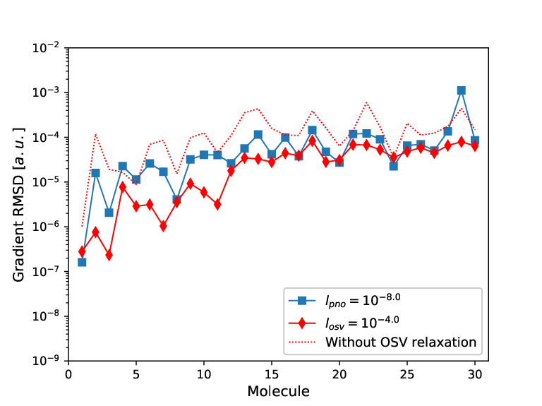
To assess the convergence of OSV-MP2 gradients with respect to the OSV selection thresholds, the RMSDs between the gradients of OSV-MP2 and RI-MP2 reference are presented in Figure 6 for molecules of varying sizes and bonding types in the Baker test setBaker 1993. As shown in Figure 6(a), the average RMSDs among all computed molecules are $1.3\times 10^{-4}$ , $3.2\times 10^{-5}$ and $6.3\times 10^{-6}$ for $l_{osv}=10^{-3.5}$ , $10^{-4}$ and $10^{-4.5}$ , respectively. For $l_{osv}=10^{-4.0}$ , the RMSDs range from $10^{-5}$ – $10^{-7}$ for smaller molecules (the molecule number lower than 15), and increase to about $5\times 10^{-4}$ – $5\times 10^{-5}$ for larger molecules.

The effect of the OSV relaxation is illustrated in Figs. 6(b)-(d) by comparing the OSV-MP2 gradients computed with and without OSV relaxation. The OSV-MP2 analytical gradient without OSV relaxation merely considers the MO- and AO-specific gradient contributions described in Secs. 2.3.2 and 2.3.3. It is obvious that the inclusion of the OSV relaxation considerably reduces the RMSDs by an order of magnitude. For instance, with $l_{osv}=10^{-4}$ (Figure 6(c)), the average RMSDs decrease from around $10^{-4}$ to $10^{-5}$ . Nevertheless, the exclusion of OSV relaxations appears less significant when more OSVs are selected according to $l_{osv}=10^{-4.5}$ (Figure 6(d)) by which the resulting gradient RMSDs are less than $10^{-4}$ , virtually comparable to results with $l_{osv}=10^{-4}$ (Figure 6(c)).

The gradient RMSDs of OSV-MP2 are compared with those of DLPNO-MP2 available in a recent publicationPinski and Neese 2019. To be as consistent as possible with the corresponding PNO thresholds ( $l_{pno}=10^{-7}$ , $10^{-8}$ and $10^{-9}$ ), we adopted the OSV threshold as $l_{osv}=\sqrt{l_{pno}}$ for comparison since the PNOs are chosen according to eigenvalues of semi-canonical pair density matrices, that is about the squared eigenvalues of the associated semi-canonical amplitudes. Nonetheless, a rigorous accuracy comparison between DLPNO-MP2 and OSV-MP2 is difficult, since at the same level of truncation (e.g, $l_{pno}=10^{-8}$ vs $l_{osv}=10^{-4}$ ) nondiagonal pair amplitudes are represented in a much more compact basis in the DLPNO approach than in the OSV approach.

As seen in Figure 6(b) by comparing loose OSVs and PNOs, the RMSDs of two methods are generally similar especially for larger molecules, yet with marginally better performance for OSV-MP2 than DLPNO-MP2 for smaller molecules. For $l_{osv}=10^{-4.5}$ / $l_{pno}=10^{-9}$ in Figure 6(d), the RMSDs of OSV-MP2 are remarkably smaller than those of DLPNO-MP2. We note that benzidine ( molecule 29) is peculiar here for DLPNO-MP2 with an RMSD above $10^{-4}$ even using $l_{pno}=10^{-9}$ . The OSV-MP2 analytical gradient however yields no significant RMSDs which are consistently below $10^{-4}$ and $10^{-5}$ for $l_{osv}=10^{-4.0}$ and $10^{-4.5}$ .

3.2 Optimized molecular structures

Bond lengths

The statistical errors of OSV-MP2 bond lengths relative to the reference data of RI-MP2 are summarized in Table 1. For all basis sets, tighter OSV thresholds lead to decreased errors of bond lengths. Notably, the OSV-MP2 optimization with $l_{osv}=10^{-4}$ is sufficiently accurate and increasing basis set sizes only slightly increases MAEs. However, the calculations with $l_{osv}=10^{-3}$ yields much larger errors.

Table 1: Mean error (ME), mean absolute error (MAE) and the maximum error (max) in bond lengths (pm) of selected Baker test molecules.

$l_{osv}$		def2-SVP	def2-TZVPP	def2-QZVPP
$10^{-3}$	ME	0.071	0.097	0.151
	MAE	0.081	0.166	0.167
	max	0.380	0.570	0.620
$10^{-4}$	ME	0.009	0.013	0.016
	MAE	0.014	0.017	0.019
	max	0.050	0.070	0.080
$10^{-5}$	ME	0.000	-0.002	0.005
	MAE	0.009	0.016	0.012
	max	0.040	0.080	0.060

In Figure 9(a), the MAEs of bond lengths with different basis sets and OSV/PNO selection thresholds are compared between OSV-MP2, PNO-MP2 and DLPNO-MP2. DLPNO-MP2 yields lower MAEs than OSV-MP2 with the loose threshold for all basis sets, but is overtaken by OSV-MP2 with tighter thresholds. For def2-TZVPP and loose threshold, the MAE for OSV-MP2 is significantly lower than PNO-MP2 by around 0.3 pm, but larger than DLPNO-MP2. The performances of the three methods are comparable for normal and tight calculations.

By repeating the OSV-MP2 geometry optimization, the long interatomic distances of noncovalent bonds have been examined in Table 2. We have chosen DTFS and RESVAN molecules out of LB12 set for which the DLPNO-MP2 optimized Si-N and S-S bond distances report quite large errors in Ref.Pinski and Neese 2019. All electrons are correlated in OSV-MP2 calculations, and both OSV-MP2 geometries are well converged for three OSV-MP2 thresholds. It is observed that $l_{osv}=10^{-4.5}$ is necessary in order to reduce the errors below 1.0 pm. However, $l_{osv}=10^{-4.0}$ appears to be sufficient for achieving relative deviations below $1\%$ , which is acceptable for such long bond distances. In general, the OSV-MP2 outperforms DLPNO-MP2 for loose selection, and both methods are comparable for normal and tight selections.

Table 2: Comparisons of the optimized interatomic distances in DTFS and RESVAN molecules between OSV-MP2 and DLPNO-MP2. The long noncovalent interatomic distances are specified in Ref.Pinski and Neese 2019

^a Predefined in Figure 9.
		DTFS (Si-N)		RESVAN (S-S)
	Threshold^a	$\Delta$ r (pm)	r_RI-MP2 (pm)	$\Delta$ r (pm)	r_RI-MP2 (pm)
DLPNO-MP2^b	Loose	1.94	214.91^b	9.36	390.66^b
	Normal	0.78		2.98
	Tight	0.33		0.91
OSV-MP2^b	Loose	0.70	211.80^c	6.90	385.80^c
	Normal	0.40		2.70
	Tight	0.00		0.80
^b DLPNO-MP2 results with frozen core approximation from Ref.Pinski and Neese 2019.
^c Our results without frozen core approximation.

Bond and dihedral angles

The errors of bond angles are reported in Table 3 for selected Baker’s test molecules according to the specification in Ref.Frank et al. 2017. In general, the MAEs are smaller than $0.1^{\circ}$ for $l_{osv}$ all values in combination with all basis sets. $l_{osv}=10^{-3}$ results in relatively large maximum errors about $1.0^{\circ}$ . Both $l_{osv}=10^{-4}$ and $10^{-5}$ substantially reduce the maximum errors by about an order of magnitude and are recommended for accurate structure optimizations. The performances of OSV-MP2, PNO-MP2 and DLPNO-MP2 in bond angles are compared in Figure 9(b). Most notably PNO-MP2 without the PNO relaxation yields larger errors than OSV-MP2 and DLPNO-MP2, in particular for def2-TZVPP and def2-QZVPP basis sets. The performances of OSV-MP2 and DLPNO-MP2 are similar with normal and tight thresholds.

Table 3: Mean absolute error (MAE) and the maximum error (max) in bond angles (^∘) of selected Baker test molecules.

$l$ _osv		def2-SVP	def2-TZVPP	def2-QZVPP
$10^{-3}$	MAE	0.05	0.08	0.10
	max	1.10	0.80	1.00
$10^{-4}$	MAE	0.02	0.03	0.03
	max	0.10	0.10	0.20
$10^{-5}$	MAE	0.02	0.03	0.02
	max	0.10	0.30	0.20

The dihedral angles of benzidine molecule are compared between OSV-MP2, PNO-MP2 and DLPNO-MP2 in Table 4. Overall, OSV-MP2 performs much better than PNO-MP2 and DLPNO-MP2 for all thresholds and basis sets, and the deviations from RI-MP2 dihedral angles are less than $0.2^{\circ}$ for OSV-MP2/normal and OSV-MP2/tight.

Table 4: Dihedral angles of benzidine for OSV-MP2, PNO-MP2 and DLPNO-MP2 with the basis sets of def2-TZVPP and def2-QZVPP.

^a Predefined in Figure 9.
Basis set	Threshold^a	RI-MP2	OSV-MP2	PNO-MP2^b	DLPNO-MP2
def2-SVP	Loose	138.8	137.2	-	-^c
	Normal		138.7	-	137.5
	Tight		138.7	-	137.6
def2-TZVPP	Loose	142.2	139.9	92.6	-^c
	Normal		142.0	143.2	138.9
	Tight		142.2	142.3	139.3
def2-QZVPP	Loose	142.1	138.7	138.4	-^c
	Normal		141.9	141.3	139.2
	Tight		142.1	140.6	139.5
^b PNO-MP2 results without PNOs relaxation from Ref.Frank et al. 2017.
^c DLPNO-MP2 reported not converged.

Performance with pair screening

The use of pair screening can considerably accelerate the OSV-MP2 calculations by discarding the pairs of occupied orbitals that make little contribution to the total correlation energy. By exploring the orbital locality and the definition of OSVs, the OSV overlap matrix elements associated with a pair $(i,j)$ exhibit an exponential decay with the separation between $i$ and $j$ . Therefore the relevant pairs entering OSV-MP2 calculations are chosen according to the previous simple schemeYang et al. 2011 in which the renormalized OSV overlap matrix is computed for a given $(i,j)$ pair and compared to a predefined pair screening threshold $l_{pair}$ . When a looser $l_{pair}$ (greater value) is used, more orbital pairs will be screened and not participate in the OSV-MP2 energy and gradient computation. The MAEs of bond lengths, bond angles and dihedral angles are reported with respect to $l_{pair}$ in Table 5. It is shown that the MAEs at $l_{pair}=10^{-4}$ are similar to those without pair screening for both bond lengths and angles. However, there is a significant increase of MAEs as $l_{pair}$ is increased from $10^{-4}$ to $10^{-2}$ . Interestingly, for dihedral angles, the errors for all $l_{pair}$ thresholds are less than $0.8^{\circ}$ .

Table 5: Mean absolute error (MAE) of bond lengths, bond angles and absolute error (AE) of dihedral angles with respect to pair screening thresholds.

	Bond length	Bond angle	Dihedral angle
$l_{pair}$	MAE (pm)	MAE (^∘)	AE (^∘)
$10^{-2}$	0.043	0.043	0.6
$10^{-3}$	0.021	0.028	0.3
$10^{-4}$	0.019	0.023	0.5
0	0.019	0.025	0.2

Timing comparison

We finally compare the elapsed times between RI-MP2, DLPNO-MP2 and OSV-MP2 for both energy and gradient evaluations on a single CPU. For all molecules considered in Table 6, our current OSV-MP2 implementation achieves speedups of 3-10 folds for gradients and 0.4-4.0 for energies compared to RI-MP2, respectively. In particular, the OSV-MP2 gradient computation is faster than RI-MP2 by an order of magnitude for the longest molecule (Gly)₁₄. For Nonactin molecule similar to (Gly)₁₄ in size, OSV-MP2 gradient calculation exhibits a poorer speedup than (Gly)₁₄ due to more kept pairs of Nonactin (6737 out of 20100 pairs) than (Gly)₁₄ (4218 out 23220 pairs), since apparently the pair screening is less effective to the cyclic Nonactin structure than the linear (Gly)₁₄. The average pair domain sizes of Nonactin and (Gly)₁₄ are similar, i.e., both own 96 OSVs, which is much larger than DLPNO pair domains (about 17-20 PNOs). On the other hand, DLPNO-MP2 retains 14937 and 8192 pairs for (Gly)₁₄ and Nonactin, respectively, that are much larger than those of OSV-MP2. Moreover, the OSV-MP2 energy and gradient scalings are $N^{2.74}$ and $N^{2.96}$ , respectively, as shown in Figure S1. This is still higher than DLPNO-MP2 and leads to longer elapsed time than DLPNO-MP2 by nearly 2 folds for large glycine chains. However, for smaller molecules, OSV-MP2 gradient computation can be 2 times faster than DLPNO-MP2, which makes it attractive for driving efficient BOMD simulations on molecules of similar size.

Table 6: Timing comparisons for polyglycine chains (Gly)_n and Nonactin (C₄₀H₆₄O₁₂) with respect to the number of basis (

N

) and auxiliary functions (

N_{aux}

) between RI-MP2 and OSV-MP2 computations. Elapsed times (minutes) of a single-point energy and gradient are reported for each molecule in the first and second row entry, respectively. Percentages of correlation energy recovery are reported for DLPNO-MP2 and OSV-MP2 as the first and second element in the last Column, respectively. These calculations were carried out serially on a single CPU (Intel Xeon E5-2640 v3@2.60GHz) with def2-TZVP basis.

l_{osv}=10^{-4}

and

l_{pair}=10^{-3}

were used for OSV selection and pair screening. RI-MP2 was performed on the quantum chemistry program ORCANeese 2018. For DLPNO-MP2/RIJCOSX, TCutPNO=

10^{-8}

and TCutDO=

10^{-2}

were set for constructing PNOs and associated PAO domains with Foster-Boys localizationFoster and Boys 1960, respectively.

Molecules	$N$	$N_{aux}$	RI-MP2	DLPNO-MP2	OSV-MP2	Speedups	Percentages
(Gly)₄	611	1502	2	7	6	0.4	99.96%, 99.96%
			49	28	14	3.5
(Gly)₆	895	2200	14	14	15	0.9	99.96%, 99.95%
			163	65	40	4.1
(Gly)₈	1179	2898	53	22	32	1.7	99.96%, 99.95%
			475	112	90	5.3
(Gly)₁₀	1463	3596	145	30	65	2.2	99.95%, 99.95%
			1069	171	198	5.4
(Gly)₁₂	1747	4294	355	39	112	3.2	99.95%, 99.95%
			2796	243	332	8.4
(Gly)₁₄	2031	4992	751	52	194	3.9	99.95%, 99.95%
			5937	328	569	10.4
Nonactin	1996	4912	598	135	198	3.0	99.91%, 99.89%
			4728	598	697	6.8

4 OSV-MP2-DRIVEN AB-INITIO BOMD

4.1 Protonated Eigen and Zundel water cations

We have performed the constant $NVE$ simulation for protonated Eigen (H₉O₄⁺) and Zundel water cluster (H₁₃O₆⁺). They are not only structural units of biological and chemical significance, but also the benchmark systems that have been extensively used to establish accuracy of other theories.

Energy drifts

In OSV-MP2 $NVE$ simulation, the OSV-MP2 approximated trajectories propagate according to the numerical integration over a finite time step which may break the energy conservation by a range of drifts at long simulation time. Therefore such drifts must be examined carefully with respect to both OSV and pair selections. The results are reported in Table 7 for benchmarking OSV-MP2 BOMD accuracy. When no pairs are screened ( $l_{pair}=0.0$ ), all energy drifts are very small. The total energies of all OSV-MP2/10 ps trajectories with $l_{osv}=10^{-3}$ are conserved within 1.0 kJ/mol, the energy drifts are substantially reduced with $l_{osv}=10^{-4}$ by two and one orders of magnitude for H₉O₄⁺ and H₁₃O₆⁺, respectively. The RMSDs, which measure the time-dependent energy fluctuation statistically, are as small as half kJ/mol for $l_{osv}=10^{-3}$ and $0.1$ – $0.2$ kJ/mol for $l_{osv}=10^{-4}$ . The difference of the computed $T_{\mathrm{av}}$ between $l_{osv}=10^{-3}$ and $l_{osv}=10^{-4}$ is about 1 K for H₉O₄⁺ and 5 K for H₁₃O₆⁺, respectively.

Table 7 suggests that the use of pair screenings yields larger statistical errors than the OSV selection. Nevertheless, a proper combination of selected $l_{osv}$ and $l_{pair}$ can produce results of acceptable accuracy. For instance, for $l_{osv}=10^{-4}$ , the choice of the medium pair screening $l_{pair}=0.001$ does not lead to significant shifts of energy (both $\delta E$ and RMSD) and temperature. However, with $l_{pair}=0.01$ and $l_{pair}=0.02$ , the energy conservation is not well sustained. As seen in Figure S2, with more pair screenings for Zundel cluster, the $l_{osv}=10^{-4}/l_{pair}=0.01$ simulation after about 4.5 ps leads to a hotter Zundel cation by 1 kJ/mol, probably arising from a more drastic change of the number of the kept pairs with time.

Table 7: Comparison of statistical energy conservation properties with respect to OSV and pair selections for

NVE

/6-31+g(d,p) simulation.

T_{\mathrm{av}}

is the average temperature computed according to the equipartition theorem for the average kinetic energy.

\delta E

is the energy drift that is the difference of the linear least-square fit to all energies at the first and last time step. RMSDs are given among all energies relative to this linear fit.

Molecule	$l_{osv}$	$l_{pair}$	$T_{\mathrm{av}}$ (K)	$\delta E$ (kJ/mol)	RMSD (kJ/mol)
H₉O ${}_{4}^{+}$	$10^{-3}$	0.000	149.3	-0.45	0.41
	$10^{-3}$	0.001	149.9	-0.50	0.40
	$10^{-3}$	0.010	152.0	0.94	0.65
	$10^{-3}$	0.020	152.1	1.21	1.21
	$5.0\times 10^{-4}$	0.000	149.3	0.36	0.32
	$10^{-4}$	0.000	150.4	0.00	0.17
	$10^{-4}$	0.001	149.5	-0.04	0.18
	$10^{-4}$	0.010	150.8	0.08	0.13
	$10^{-4}$	0.020	149.1	0.08	0.14
H₁₃O ${}_{6}^{+}$	$10^{-3}$	0.000	153.0	-0.98	0.55
	$10^{-3}$	0.001	191.1	50.97	16.14
	$5.0\times 10^{-4}$	0.000	146.6	-0.02	0.21
	$10^{-4}$	0.000	148.5	0.06	0.22
	$10^{-4}$	0.001	149.2	-0.04	0.25
	$10^{-4}$	0.010	150.3	1.57	0.62
	$10^{-4}$	0.020	150.0	-0.53	0.34

Radial distribution function (RDF)

The trajectory specification of computing RDFs of the O-O and O-H distances was adopted according to the description of Ref.Li et al. 2016. As seen in Figure 14, the OSV-MP2 BOMD calculations with $l_{osv}=10^{-4}$ are capable of retrieving all O-O and O-H structural details including the RDF landscape and peak positions for both Eigen and Zundel clusters, and also in excellent agreement with the canonical MP2 BOMD reference resultsLi et al. 2016. However, for Zundel cluster, the calculations with the loose OSV selection $l_{osv}=10^{-3}$ do not well resolve two innermost peaks of the O-O RDF at about $2.4$ Å (Zundel-like O-O distance) and $2.8$ Å (Eigen-like O-O distance), but rather predict a more dominating Eigen-like solvation shell. It is demonstrated in Figure S3 that the pair screenings, when combined with the normal OSV selection $l_{osv}=10^{-4}$ , have little effects on the RDF landscapes yet with a small broadening of the RDF peaks at longer O-H and O-O distances by increasing $l_{pair}$ .

Vibrational density of states (VDOS)

Vibrational density of states are computed as the Fourier transform of the velocity autocorrelation function according to the Ref.Li et al. 2016. However, our initial structures are generated from RI-MP2 optimization, with the momentum corresponding to 300 K. We compare the computed VDOS spectra in Figures 17 and S4. The positions of significant peaks can be hardly affected by the OSV selection and pair screening. In particular, for Eigen cluster in Figures 17 (a) and S4(a), the weak peaks at about 3000 cm^-1 representing the proton stretch mode are well reproducedHaycraft et al. 2017 in all OSV-MP2 BOMD calculations. For Zundel cluster in Figures 17 (b) and S4(b), the two peaks of medium intensity around 4000 cm^-1 are clearly resolved. However, the peak intensities are largely influenced by the combined $l_{osv}$ and $l_{pair}$ . For instance, the peaks at both low and high frequency regions are relatively intensified by decreasing $l_{osv}$ . On the other hand, a large pair screening appears to substantially weaken the 4000 cm^-1 peak at the lower frequency side.

4.2 Rotational free energy of ethanol

The OSV-MP2/cc-pvTZ $NVT$ simulations were carried out for computing the rotational free energies of the coupled hydroxyl and methyl groups in ethanol molecule at 300 K. The $NVT$ simulation features thermal energy exchange which may compensate the electronic energy loss due to selected OSVs through adding a thermostat into Hamiltonian for coupling the system and reservoir. This thus opens up the feasibility of making OSV-MP2 BOMD available for simulating systems at a finite temperature. However, the detailed investigation on the interplay between the thermal coupling and the OSV selection is not the subject of this work and will be probed in future applications. In the current work, the Nosé-Hoover thermostat was employed with the temperature coupling time constant of 100 fs. The simulation temperature is conserved within a drift of only -0.051 K for $l_{osv}=10^{-4}$ and $l_{pair}=0.0$ .

Ethanol can exist in two conformers, the trans-ethanol with the hydroxyl group trans to the methyl group, and the gauche-ethanol with the hydroxyl group gauche to the methyl group. The gauche-ethanol stability computed by single point DFT is close to the trans-ethanol by, for instances, 0.01 kcal/mol for B3LYP/cc-pVTZDurig et al. 2011 and -0.08 kcal/mol PBE-TS/cc-pVTZChmiela et al. 2018. Our OSV-MP2/cc-pVTZ $NVT$ simulation predicts that the trans-ethanol conformer is more stable than the gauche-ethanol conformer by 0.22 kcal/mol, as shown in Figure 18. The OSV-MP2/cc-pVTZ $NVT$ also finds the free energy barriers of 1.00 kcal/mol and 0.62 kcal/mol to the hydroxyl rotation and trans-to-gauge transformation, respectively. Recently, Chmiela et al.Chmiela et al. 2018; Sauceda et al. 2019 reported that the corresponding CCSD(T) barriers are 0.11 kcal/mol, 1.30 kcal/mol and 1.18 kcal/mol, by training the symmetrized gradient-domain machine learning (sGDML) model for the CCSD(T) force field in MD simulations. It was observed however that the gauche is more stable than the trans by repeating the same calculation with sGDML@DFT(PBE-TS)Chmiela et al. 2018. Compared to sGDML@CCSD(T), our OSV-MP2 simulation seems to underestimate the energy level of the transition state for tran-to-gauche transformation by 0.56 kcal/mol. This disagreement may be ascribed to the difference of the levels in describing electron correlations between MP2 and CCSD(T) methods. Nevertheless, single point calculationsDyczmons 2004 corresponding to 0 K show that the energy barriers are in fact similar between MP2 and CCSD(T), with differences of only a few hundredth kcal/mol. Therefore it remains a question whether such a subtle difference of electron correlation between MP2 and CCSD(T) for ethanol has any significance due to a thermal fluctuation of $\approx 0.6$ kcal/mol at 300 K. More importantly, we realize that in our computational setting for metadynamics simulation, a relatively large time constant of 100 fs was used in order to achieve a small temperature drift ( $\approx-0.051$ K) and avoid poor coupling in a long time equilibration. However, this inevitably results in a more wild distribution of Nosé-Hoover frequencies and thus a larger thermal fluctuation. More detailed studies on this issue within the OSV-MP2 framework are underway.

5 CONCLUSIONS

In this work, we have described the algorithm and implementation for analytically computing the energy derivatives from all OSV-MP2 energy contributions with local molecular orbitals. We have shown that it is possible to evaluate the OSV relaxation by explicitly solving non-degenerate perturbed eigenvalue problem in which exact OSV rotations can be implemented between the retained and discarded OSV subspaces. The simplicity of the OSV construction leads to the block-diagonal structure of pair-specific OSV relaxation matrix which decouples OSV rotations within a single orbital pair. The solution of pair-specific OSV relaxation elements enters the source of a single Z-vector equation along with the MO relaxation and the localization constraint, as solved in a conventional way that is independent of the degrees of freedom.

The accuracy of this approach has been benchmarked on a set of well studied molecules for optimized geometries and molecular dynamics simulations. The OSV relaxation effects are significant and can be recovered with the normal OSV selection for practical use of reproducing canonical RI-MP2 molecular structures. Moreover, the classical molecular dynamics with OSV-MP2 input gradients has been implemented. It has been demonstrated that using a normal OSV selection, all major peaks of the O-O/O-H radial distribution functions and vibrational densities of states for protonated water tetramer and hexamer can be well identified. A 200 ps well-tempered metadynamics simulation with OSV-MP2 gradients at 300 K has been shown to be capable of distinguishing the gauche and trans conformers of ethanol molecule.

There is much to explore for improving the current implementation by noting the aspects as follows. (1) Solving the Z-vector equation and two-electron integral transformation therein in MO basis become one bottleneck step for large molecules. (2) The evaluation of energy gradients through Eq. () does not yet take advantage of OSV savings and therefore scales quickly with system sizes. (3) Embarrassing parallelization schemes seem obvious within the OSV-MP2 framework by distributing local orbitals over many processes. (4) Finally, the OSV-MP2 gradient computation is currently much slower than OSV-MP2 energy by 3-4 folds. An appropriate scheme for pruning out insignificant OSV relaxations and associated pairs shall further speed up gradient computation. The efforts along these directions are being made and will be reported in future.

J.Y. acknowledges financial supports from the Hong Kong Research Grant Council (RGC) Early Career Scheme (ECS) through Grant No. ECS27307517, and the Hui’s fund provided by department of chemistry at the University of Hong Kong. R.Y.Z. thanks Prof. Roberto Car for hosting his summer research and valuable discussions. J.Y. thanks Dr. Qiming Sun for general assistance in PySCF package.

The file Supporting supporting.pdf contains further results of the computations and is available free of charge.

References

Zaleśny et al. (2011) Zaleśny, R.; Papadopoulos, M. G.; Mezey, P. G.; Leszczynski, J. Linear-Scaling Techniques in Computational Chemistry and Physics: Methods and Applications; Springer Science & Business Media, 2011; Vol. 13.
Gordon (2017) Gordon, M. S. Fragmentation: Toward Accurate Calculations on Complex Molecular Systems; John Wiley & Sons, 2017.
Martinez and Carter (1994) Martinez, T. J.; Carter, E. A. Pseudospectral Møller–Plesset perturbation theory through third order. J. Chem. Phys. 1994, 100, 3631–3638.
Ayala and Scuseria (1999) Ayala, P. Y.; Scuseria, G. E. Linear scaling second-order Møller–Plesset theory in the atomic orbital basis for large molecular systems. J. Chem. Phys. 1999, 110, 3660–3671.
Reynolds et al. (1996) Reynolds, G.; Martinez, T. J.; Carter, E. A. Local weak pairs spectral and pseudospectral singles and doubles configuration interaction. J. Chem. Phys. 1996, 105, 6455–6470.
Lee et al. (2000) Lee, M. S.; Maslen, P. E.; Head-Gordon, M. Closely approximating second-order Mo/ller–Plesset perturbation theory with a local triatomics in molecules model. J. Chem. Phys. 2000, 112, 3592–3601.
Pulay (1983) Pulay, P. Localizability of dynamic electron correlation. Chem. Phys. Lett. 1983, 100, 151–154.
Sæbø and Pulay (1985) Sæbø, S.; Pulay, P. Local configuration interaction: An efficient approach for larger molecules. Chem. Phys. Lett. 1985, 113, 13–18.
Sæbø and Pulay (1987) Sæbø, S.; Pulay, P. Fourth-order Møller–Plessett perturbation theory in the local correlation treatment. I. Method. J. Chem. Phys. 1987, 86, 914–922.
Sæbø and Pulay (1993) Sæbø, S.; Pulay, P. Local treatment of electron correlation. Annu. Rev. Phys. Chem. 1993, 44, 213–236.
Hampel and Werner (1996) Hampel, C.; Werner, H.-J. Local treatment of electron correlation in coupled cluster theory. J. Chem. Phys. 1996, 104, 6286–6297.
Schütz and Werner (2000) Schütz, M.; Werner, H.-J. Local perturbative triples correction (T) with linear cost scaling. Chem. Phys. Lett. 2000, 318, 370–378.
Schütz and Werner (2001) Schütz, M.; Werner, H.-J. Low-order scaling local electron correlation methods. IV. Linear scaling local coupled-cluster (LCCSD). J. Chem. Phys. 2001, 114, 661–681.
Schütz (2002) Schütz, M. Low-order scaling local electron correlation methods. V. Connected triples beyond (T): Linear scaling local CCSDT-1b. J. Chem. Phys. 2002, 116, 8772–8785.
Schütz (2002) Schütz, M. A new, fast, semi-direct implementation of linear scaling local coupled cluster theory. Phys. Chem. Chem. Phys. 2002, 4, 3941–3947.
Werner and Schütz (2011) Werner, H.-J.; Schütz, M. An efficient local coupled cluster method for accurate thermochemistry of large systems. J. Chem. Phys. 2011, 135, 144116.
Meyer (1971) Meyer, W. Ionization energies of water from PNO-CI calculations. Int. J. Quantum Chem. 1971, 5, 341–348.
Ahlrichs et al. (1975) Ahlrichs, R.; Lischka, H.; Staemmler, V.; Kutzelnigg, W. PNO–CI (pair natural orbital configuration interaction) and CEPA–PNO (coupled electron pair approximation with pair natural orbitals) calculations of molecular systems. I. Outline of the method for closed-shell states. J. Chem. Phys. 1975, 62, 1225–1234.
Neese et al. (2009) Neese, F.; Hansen, A.; Liakos, D. G. Efficient and accurate approximations to the local coupled cluster singles doubles method using a truncated pair natural orbital basis. J. Chem. Phys. 2009, 131, 064103.
Yang et al. (2011) Yang, J.; Kurashige, Y.; Manby, F. R.; Chan, G. K. Tensor factorizations of local second-order Møller–Plesset theory. J. Chem. Phys. 2011, 134, 044123.
Kurashige et al. (2012) Kurashige, Y.; Yang, J.; Chan, G. K.-L.; Manby, F. R. Optimization of orbital-specific virtuals in local Møller–Plesset perturbation theory. J. Chem. Phys. 2012, 136, 124106.
Yang et al. (2012) Yang, J.; Chan, G. K.-L.; Manby, F. R.; Schütz, M.; Werner, H.-J. The orbital-specific-virtual local coupled cluster singles and doubles method. J. Chem. Phys. 2012, 136, 144105.
Schütz et al. (2013) Schütz, M.; Yang, J.; Chan, G. K.-L.; Manby, F. R.; Werner, H.-J. The orbital-specific virtual local triples correction: OSV–L(T). J. Chem. Phys. 2013, 138, 054109.
Krause and Werner (2012) Krause, C.; Werner, H.-J. Comparison of explicitly correlated local coupled–cluster methods with various choices of virtual orbitals. Phys. Chem. Chem. Phys. 2012, 14, 7591–7604.
Riplinger and Neese (2013) Riplinger, C.; Neese, F. An efficient and near linear scaling pair natural orbital based local coupled cluster method. J. Chem. Phys. 2013, 138, 034106.
Riplinger et al. (2013) Riplinger, C.; Sandhoefer, B.; Hansen, A.; Neese, F. Natural triple excitations in local coupled cluster calculations with pair natural orbitals. J. Chem. Phys. 2013, 139, 134101.
Schmitz et al. (2013) Schmitz, G.; Helmich, B.; Hättig, C. A scaling PNO–MP2 method using a hybrid OSV–PNO approach with an iterative direct generation of OSVs. Mol. Phys. 2013, 111, 2463–2476.
Werner et al. (2015) Werner, H.-J.; Knizia, G.; C., K.; Schwilk, M.; Dornbach, M. Scalable electron correlation methods. I. PNO–LMP2 with linear scaling in the molecular size and near–inverse–linear scaling in the number of processors. J. Chem. Theory Comput. 2015, 11, 484––507.
Schmitz et al. (2014) Schmitz, G.; Hättig, C.; Tew, D. P. Explicitly correlated PNO-MP2 and PNO-CCSD and their application to the S66 set and large molecular systems. Phys. Chem. Chem. Phys. 2014, 16, 22167–22178.
Schmitz and Hättig (2016) Schmitz, G.; Hättig, C. Perturbative triples correction for local pair natural orbital based explicitly correlated CCSD (F12*) using Laplace transformation techniques. J. Chem. Phys. 2016, 145, 234107.
Pavošević et al. (2016) Pavošević, F.; Pinski, P.; Riplinger, C.; Neese, F.; Valeev, E. F. Sparse Maps-A systematic infrastructure for reduced-scaling electronic structure methods. IV. Linear-scaling second-order explicitly correlated energy with pair natural orbitals. J. Chem. Phys. 2016, 144, 144109.
Pavošević et al. (2017) Pavošević, F.; Peng, C.; Pinski, P.; Riplinger, C.; Neese, F.; Valeev, E. F. Sparse Maps-A systematic infrastructure for reduced scaling electronic structure methods. V. Linear scaling explicitly correlated coupled-cluster method with pair natural orbitals. J. Chem. Phys. 2017, 146, 174108.
Ma et al. (2017) Ma, Q.; Schwilk, M.; Köppl, C.; Werner, H.-J. Scalable electron correlation methods. 4. Parallel explicitly correlated local coupled cluster with pair natural orbitals (PNO-LCCSD-F12). J. Chem. Theory Comput. 2017, 13, 4871–4896.
Ma and Werner (2018) Ma, Q.; Werner, H.-J. Scalable Electron Correlation Methods. 5. Parallel Perturbative Triples Correction for Explicitly Correlated Local Coupled Cluster with Pair Natural Orbitals. J. Chem. Theory Comput. 2018, 14, 198–215.
Saitow et al. (2017) Saitow, M.; Becker, U.; Riplinger, C.; Valeev, E. F.; Neese, F. A new near-linear scaling, efficient and accurate, open-shell domain-based local pair natural orbital coupled cluster singles and doubles theory. J. Chem. Phys. 2017, 146, 164105.
Demel et al. (2015) Demel, O.; Pittner, J.; Neese, F. A local pair natural orbital-based multireference Mukherjee’s coupled cluster method. J. Chem. Theory Comput. 2015, 11, 3104–3114.
Guo et al. (2016) Guo, Y.; Sivalingam, K.; Valeev, E. F.; Neese, F. SparseMaps-A systematic infrastructure for reduced-scaling electronic structure methods. III. Linear-scaling multireference domain-based pair natural orbital N-electron valence perturbation theory. J. Chem. Phys. 2016, 144, 094111.
Menezes et al. (2016) Menezes, F.; Kats, D.; Werner, H.-J. Local complete active space second-order perturbation theory using pair natural orbitals (PNO-CASPT2). J. Chem. Phys. 2016, 145, 124115.
Brabec et al. (2018) Brabec, J.; Lang, J.; Saitow, M.; Pittner, J.; Neese, F.; Demel, O. Domain-Based Local Pair Natural Orbital Version of Mukherjee’s State-Specific Coupled Cluster Method. J. Chem. Theory Comput. 2018, 14, 1370–1382.
Lang et al. (2019) Lang, J.; Brabec, J.; Saitow, M.; Pittner, J.; Neese, F.; Demel, O. Perturbative triples correction to Domain-based Local Pair Natural Orbital variant of Mukherjee’s state specific coupled cluster method. Phys. Chem. Chem. Phys. 2019,
Helmich and Haettig (2013) Helmich, B.; Haettig, C. A pair natural orbital implementation of the coupled cluster model CC2 for excitation energies. J. Chem. Phys. 2013, 139, 084114.
Frank and Hättig (2018) Frank, M. S.; Hättig, C. A pair natural orbital based implementation of CCSD excitation energies within the framework of linear response theory. J. Chem. Phys. 2018, 148, 134102.
Peng et al. (2018) Peng, C.; Clement, M. C.; Valeev, E. F. State-Averaged Pair Natural Orbitals for Excited States: A Route toward Efficient Equation of Motion Coupled-Cluster. J. Chem. Theory Comput. 2018, 14, 5597–5607.
Helmich and Hättig (2011) Helmich, B.; Hättig, C. Local pair natural orbitals for excited states. J. Chem. Phys. 2011, 135, 214106.
Helmich and Hättig (2014) Helmich, B.; Hättig, C. A pair natural orbital based implementation of ADC (2)-x: Perspectives and challenges for response methods for singly and doubly excited states in large molecules. Comput. Theor. Chem. 2014, 1040, 35–44.
Pulay (1969) Pulay, P. Ab initio calculation of force constants and equilibrium geometries in polyatomic molecules: I. Theory. Mol. Phys. 1969, 17, 197–204.
Yamaguchi (1994) Yamaguchi, Y. A new dimension to quantum chemistry: analytic derivative methods in ab initio molecular electronic structure theory; Oxford University Press, USA, 1994.
Weigend and Häser (1997) Weigend, F.; Häser, M. RI-MP2: first derivatives and global consistency. Theor. Chem. Acc. 1997, 97, 331–340.
Hättig et al. (2006) Hättig, C.; Hellweg, A.; Köhn, A. Distributed memory parallel implementation of energies and gradients for second-order Møller–Plesset perturbation theory with the resolution-of-the-identity approximation. Phys. Chem. Chem. Phys. 2006, 8, 1159–1169.
Lochan et al. (2007) Lochan, R. C.; Shao, Y.; Head-Gordon, M. Quartic-Scaling Analytical Energy Gradient of Scaled Opposite-Spin Second-Order Møller–Plesset Perturbation Theory. J. Chem. Theory Comput. 2007, 3, 988–1003.
Distasio Jr et al. (2007) Distasio Jr, R. A.; Steele, R. P.; Head-Gordon, M. The analytical gradient of dual-basis resolution-of-the-identity second-order Møller–Plesset perturbation theory. Mol. Phys. 2007, 105, 2731–2742.
Distasio Jr et al. (2007) Distasio Jr, R. A.; Steele, R. P.; Rhee, Y. M.; Shao, Y.; Head-Gordon, M. An improved algorithm for analytical gradient evaluation in resolution-of-the-identity second-order Møller–Plesset perturbation theory: Application to alanine tetrapeptide conformational analysis. J. Comput. Chem. 2007, 28, 839–856.
Schweizer et al. (2008) Schweizer, S.; Doser, B.; Ochsenfeld, C. An atomic orbital-based reformulation of energy gradients in second-order Møller–Plesset perturbation theory. J. Chem. Phys. 2008, 128, 154101.
Kristensen et al. (2012) Kristensen, K.; Jørgensen, P.; Jansík, B.; Kjærgaard, T.; Reine, S. Molecular gradient for second-order Møller–Plesset perturbation theory using the divide-expand-consolidate (DEC) scheme. J. Chem. Phys. 2012, 137, 114102.
Adamowicz et al. (1984) Adamowicz, L.; Laidig, W.; Bartlett, R. Analytical gradients for the coupled-cluster method. Int. J. Quantum Chem. 1984, 26, 245–254.
Fitzgerald et al. (1985) Fitzgerald, G.; Harrison, R.; Laidig, W. D.; Bartlett, R. J. Analytical gradient evaluation in coupled-cluster theory. Chem. Phys. Lett. 1985, 117, 433–436.
Scheiner et al. (1987) Scheiner, A. C.; Scuseria, G. E.; Rice, J. E.; Lee, T. J.; Schaefer III, H. F. Analytic evaluation of energy gradients for the single and double excitation coupled cluster (CCSD) wave function: Theory and application. J. Chem. Phys. 1987, 87, 5361–5373.
Salter et al. (1989) Salter, E.; Trucks, G. W.; Bartlett, R. J. Analytic energy derivatives in many-body methods. I. First derivatives. J. Chem. Phys. 1989, 90, 1752–1766.
Scuseria (1991) Scuseria, G. E. Analytic evaluation of energy gradients for the singles and doubles coupled cluster method including perturbative triple excitations: Theory and applications to FOOF and Cr₂. J. Chem. Phys. 1991, 94, 442–447.
Hald et al. (2003) Hald, K.; Halkier, A.; Jørgensen, P.; Coriani, S.; Hättig, C.; Helgaker, T. A Lagrangian, integral-density direct formulation and implementation of the analytic CCSD and CCSD (T) gradients. J. Chem. Phys. 2003, 118, 2985–2998.
Bozkaya and Sherrill (2017) Bozkaya, U.; Sherrill, C. D. Analytic energy gradients for the coupled-cluster singles and doubles with perturbative triples method with the density-fitting approximation. J. Chem. Phys. 2017, 147, 044104.
El Azhary et al. (1998) El Azhary, A.; Rauhut, G.; Pulay, P.; Werner, H.-J. Analytical energy gradients for local second-order Møller–Plesset perturbation theory. J. Chem. Phys. 1998, 108, 5185–5193.
Schütz et al. (2004) Schütz, M.; Werner, H.-J.; Lindh, R.; Manby, F. R. Analytical energy gradients for local second-order Møller–Plesset perturbation theory using density fitting approximations. J. Chem. Phys. 2004, 121, 737–750.
Ledermüller and Schütz (2014) Ledermüller, K.; Schütz, M. Local CC2 response method based on the Laplace transform: Analytic energy gradients for ground and excited states. J. Chem. Phys. 2014, 140, 164113.
Rauhut and Werner (2001) Rauhut, G.; Werner, H.-J. Analytical energy gradients for local coupled-cluster methods. Phys. Chem. Chem. Phys. 2001, 3, 4853–4862.
McAlexander and Crawford (2015) McAlexander, H. R.; Crawford, T. D. A comparison of three approaches to the reduced-scaling coupled cluster treatment of non-resonant molecular response properties. J. Chem. Theory Comput. 2015, 12, 209–222.
Frank et al. (2017) Frank, M. S.; Schmitz, G.; Hättig, C. The PNO–MP2 gradient and its application to molecular geometry optimisations. Mol. Phys. 2017, 115, 343–356.
Datta et al. (2016) Datta, D.; Kossmann, S.; Neese, F. Analytic energy derivatives for the calculation of the first-order molecular properties using the domain-based local pair-natural orbital coupled-cluster theory. J. Chem. Phys. 2016, 145, 114101.
Pinski and Neese (2018) Pinski, P.; Neese, F. Communication: Exact analytical derivatives for the domain-based local pair natural orbital MP2 method (DLPNO-MP2). J. Chem. Phys. 2018, 148, 031101.
Pinski and Neese (2019) Pinski, P.; Neese, F. Analytical gradient for the domain-based local pair natural orbital second order Møller–Plesset perturbation theory method (DLPNO-MP2). J. Chem. Phys. 2019, 150, 164102.
Russ and Crawford (2004) Russ, N. J.; Crawford, T. D. Potential energy surface discontinuities in local correlation methods. J. Chem. Phys. 2004, 121, 691–696.
Sun et al. (2018) Sun, Q.; Berkelbach, T. C.; Blunt, N. S.; Booth, G. H.; Guo, S.; Li, Z.; Liu, J.; McClain, J. D.; Sayfutyarova, E. R.; Sharma, S.; Wouters, S.; Chan, G. K.-L. PySCF: the Python-based simulations of chemistry framework. Wiley Interdiscip. Rev. Comput. Mol. Sci. 2018, 8, e1340.
Hylleraas (1930) Hylleraas, E. EA Hylleraas, Z. Phys. 65, 209 (1930). Z. Phys. 1930, 65, 209–225.
Trefethen and Bau III (1997) Trefethen, L. N.; Bau III, D. Numerical Linear Algebra; Siam, 1997; Vol. 50.
Saad (2011) Saad, Y. Numerical Methods For Large Eigenvalue Problems: revised edition; Siam, 2011; Vol. 66.
Pipek and Mezey (1989) Pipek, J.; Mezey, P. G. A fast intrinsic localization procedure applicable for abinitio and semiempirical linear combination of atomic orbital wave functions. J. Chem. Phys. 1989, 90, 4916–4926.
Sun and Chan (2014) Sun, Q.; Chan, G. K.-L. Exact and optimal quantum mechanics/molecular mechanics boundaries. J. Chem. Theory Comput. 2014, 10, 3784–3790.
Feyereisen et al. (1993) Feyereisen, M.; Fitzgerald, G.; Komornicki, A. Use of approximate integrals in ab initio theory. An application in MP2 energy calculations. Chem. Phys. Lett. 1993, 208, 359–363.
Weigend et al. (1998) Weigend, F.; Häser, M.; Patzelt, H.; Ahlrichs, R. RI-MP2: optimized auxiliary basis sets and demonstration of efficiency. Chem. Phys. Lett. 1998, 294, 143–152.
Baker (1993) Baker, J. Techniques for geometry optimization: A comparison of Cartesian and natural internal coordinates. J. Comput. Chem. 1993, 14, 1085–1100.
Foster and Boys (1960) Foster, J.; Boys, S. Canonical configurational interaction procedure. Rev. Mod. Phys 1960, 32, 300.
Neese (2018) Neese, F. Software update: the ORCA program system, version 4.0. Wiley Interdiscip. Rev. Comput. Mol. Sci. 2018, 8, e1327.
Li et al. (2016) Li, J.; Haycraft, C.; Iyengar, S. S. Hybrid extended Lagrangian, post-Hartree–Fock Born–Oppenheimer ab initio molecular dynamics using fragment-based electronic structure. J. Chem. Theory Comput. 2016, 12, 2493–2508.
Haycraft et al. (2017) Haycraft, C.; Li, J.; Iyengar, S. S. Efficient,“On-the-Fly”, Born–Oppenheimer and Car–Parrinello-type Dynamics with Coupled Cluster Accuracy through Fragment Based Electronic Structure. J. Chem. Theory Comput. 2017, 13, 1887–1901.
Durig et al. (2011) Durig, J. R.; Deeb, H.; Darkhalil, I. D.; Klaassen, J. J.; Gounev, T. K.; Ganguly, A. The r0 structural parameters, conformational stability, barriers to internal rotation, and vibrational assignments for trans and gauche ethanol. J. Mol. Struct. 2011, 985, 202–210.
Chmiela et al. (2018) Chmiela, S.; Sauceda, H. E.; Müller, K. R.; Tkatchenko, A. Towards exact molecular dynamics simulations with machine–learned force fields. Nat. Commun. 2018, 9, 3887.
Sauceda et al. (2019) Sauceda, H. E.; Chmiela, S.; Poltavsky, I.; Müller, K.-R.; Tkatchenko, A. Molecular force fields with gradient-domain machine learning: Construction and application to dynamics of small molecules with coupled cluster forces. J. Chem. Phys. 2019, 150, 114102.
Dyczmons (2004) Dyczmons, V. Dimers of ethanol. J. Phys. Chem. A 2004, 108, 2080–2086.

A complete OSV-MP2 analytical gradient theory for molecular structure and dynamics simulations Equal contributions

Abstract

1 INTRODUCTION

2 THEORY AND IMPLEMENTATION

2.1 OSV-MP2 wavefunction

2.2 Perturbed OSVs and relaxation

2.2.1 OSV orbital rotation

2.2.2 OSV relaxation as perturbed non-degenerate eigenvalue problem

2.3 OSV-MP2 analytical gradient theory

2.3.1 OSV-specific energy gradient Ec{λ}E^{\{\lambda\}}_{c}

2.3.2 MO-specific energy gradient Ec[λ]E^{[\lambda]}_{c}

2.3.3 AO-specific energy gradient Ec(λ)E^{(\lambda)}_{c}

2.4 Implementation scheme

3 APPLICATIONS TO MOLECULAR STRUCTURES

3.1 Accuracy of OSV-MP2 analytical gradients

3.2 Optimized molecular structures

Bond lengths

Bond and dihedral angles

Performance with pair screening

Timing comparison

4 OSV-MP2-DRIVEN AB-INITIO BOMD

4.1 Protonated Eigen and Zundel water cations

Energy drifts

Radial distribution function (RDF)

Vibrational density of states (VDOS)

4.2 Rotational free energy of ethanol

5 CONCLUSIONS

References

2.3.1 OSV-specific energy gradient $E^{\{\lambda\}}_{c}$

2.3.2 MO-specific energy gradient $E^{[\lambda]}_{c}$

2.3.3 AO-specific energy gradient $E^{(\lambda)}_{c}$