Continuous-Variable Quantum Key Distribution with a Real Local Oscillator and without Auxiliary Signals

With quantum computers threatening to break the security of today’s cryptosystems, the field of quantum communications attracts increasing attention. In this field, continuous variable quantum key distribution (CV-QKD) is very attractive for a practical implementation because it is based on coherent detection and promises to require only commercial off-the-shelf components. However, one crucial difference to classical optical communications is that the received power level is usually less than $1\text{\,}\mathrm{ph}\text{/}\mathrm{bit}$ for a discrete modulation leverrier2011, translating to a signal to noise ratio (SNR) of less than $0\text{\,}\mathrm{dB}$. Additionally, residual phase noise contributes to the excess noise kleis2017, which is the critical performance parameter for CV-QKD grosshans2003. The combination of ultra low SNR and required accuracy makes carrier phase recovery the major challenge in practical CV-QKD. The first approach to deal with this challenge was to avoid phase noise by using a remote local oscillator (LO) grosshans2003; lodewyck2005; qi2007; jouguet2013. The disadvantage is that the remote LO compromises the security and limits the achievable distance jouguet2013a. Therefore, it is highly preferable that CV-QKD systems work with a real LO generated by a separate laser source at the receiver site (Bob). Since 2015, various real LO systems have been proposed and experimentally demonstrated kleis2015; huang2015; qi2015; soh2015; schrenk2016; marie2017; schrenk2017; comandar2017; laudenbach2017; wang2018. In all the proposed systems, carrier phase estimation is based on auxiliary signals, also called pilots, that are generated at the transmitter site (Alice). However, the pilots occupy additional bandwidth and significantly increase the complexity of the system. For example, the system in laudenbach2017 uses only one polarization for the quantum signal and the orthogonal one for a pilot tone. In kleis2015, two pilot tones are multiplexed with the quantum signal in the frequency domain and occupy more bandwidth than the quantum signal itself. In both cases, the spectral efficiency could at least be doubled without pilots. Another important issue is that pilot tones are not included in the current security proofs for CV-QKD fossier2009; leverrier2011. Despite all these issues, no real LO system without pilot tones has been reported up to now. Regarding the large number of pilot-based systems proposed, it appears as if pilot tones were indispensable in CV-QKD systems with a real LO. However, no convincing argument or experimental demonstration about the necessity of pilots has been made yet. The present article addresses the question of whether or not designing a CV-QKD system without pilot tones is possible with current fiber-optic technology. Our approach is to design and experimentally investigate such a CV-QKD system. In this, the quantum signal is discrete phase modulated with an order of $M=2$ or $M=4$. The latter corresponds to the most established CV-QKD protocol with a discrete modulation. A Bayesian particle smoother, which is trained using Monte Carlo Markov chain (MCMC) methods, is used for carrier phase estimation at the receiver. As particle smoothing achieves optimum tracking of dynamic variables it is very suitable to investigate the limits of carrier phase estimation in the ultra-low SNR regime. In any CV-QKD protocol, it is absolutely necessary that Alice reveals a fraction of her transmitted symbols via a public classical channel grosshans2003a. We demonstrate that these already available symbols can also be used to substantially improve the phase noise mitigation which enables pilotless CV-QKD without any loss of efficiency.

The experimental setup and digital signal processing (DSP) routine is shown in figure 1. The quantum signal is discrete phase-modulated in baseband with a modulation order $M=2$ or $M=4$ at a symbol rate of $17\text{\,}\mathrm{GBd}$. Bob uses a balanced receiver to perform heterodyne detection at an intermediate frequency of $\delta\nu_{\mathrm{AB}}\approx$10\text{\,}\mathrm{GHz}$$. In the DSP routine, Bob first down-converts the signal to baseband and applies the matched filter $h_{\mathrm{Q}}$. Then, the signal is down-sampled to 2 samples per symbol (sps) and equalized by the FIR-filter $h_{\mathrm{Eq}}$, which is tuned using the constant-modulus algorithm only once for a high SNR. Timing synchronization is performed by the digital filter and square algorithm oerder1988 followed by an extended Kalman filter that tracks the argument of the complex Fourier coefficient $X_{n}$, where $n$ is the block index of the blockwise DSP procedure. After timing correction ($h_{\mathrm{shift}}$) and down-sampling to one sample per symbol, carrier phase estimation is performed by a particle smoother. In order to find the optimum parameters $\hat{\theta}$ of the state space model, an extended Kalman filter is trained using MCMC methods sarkka2013.

The achievable key rate and distance of any CV-QKD system is very sensitive to the excess noise power $\xi_{b}$ normalized to shot noise units because it could provide information to an eavesdropper. To obtain an accurate excess noise estimate after the quantum communication, receiver noise calibration and quantum signal power estimation are required in CV-QKD. Therefore, excess noise estimation is also an important part of our experimental investigation. One can write the mean power of the received symbols $b_{k}$ as

where $P_{\mathrm{Q}}$, $P_{\mathrm{SN}}$, $P_{\mathrm{EN}}$ and $\xi_{b}$ are the quantum signal power, the shot noise power, the electrical receiver noise power and the excess noise power in arbitrary units respectively. The excess noise in shot noise units is calculated as

To calibrate $P_{\mathrm{SN}}$ and $P_{\mathrm{EN}}$, the quantum signal is deactivated. The total noise power $P_{\mathrm{SN}}+P_{\mathrm{EN}}$ and the electrical noise power $P_{\mathrm{EN}}$ are calibrated in separate measurements with activated and deactivated LO respectively. This is done after each quantum signal measurement. To estimate $P_{\mathrm{Q}}$ in our experiments, we evaluate the correlation between $a_{k}$ and $b_{k}$.

Generally in CV-QKD, to estimate $P_{\mathrm{Q}}$ and other important parameters such as the channel transmission and the mutual information shared between Alice and Bob, Alice has to reveal a randomly selected subset of her transmitted symbols $a_{k}$ after the quantum signal transmission grosshans2003a. More precisely, she publicly reveals the vector $a_{k}\cdot r_{k}$, where

That means that for each individual quantum symbol, there is a probability $p_{r}$ of being revealed after the quantum communication. As a side effect of symbol revelation, the particle smoother can take advantage of the revealed symbols to improve the accuracy of phase estimation. Depending on the value of each element $r_{k}$, the particle smoother adapts its measurement model accordingly. This means that phase estimation can only take place after Alice’s symbol revelation. However, as the sequence $\tilde{b}_{k}$ is already down-sampled to one sample per symbol, it is no additional effort to store the sequence $\tilde{b}_{k}$ compared to $b_{k}$. And since the continuous variable $b_{k}$ must be stored for error correction anyway, which takes place after Alice’s symbols have been revealed grosshans2003, this approach does not affect the feasibility nor the efficiency of the CV-QKD system in any way.

The noise calibration not only enables the excess noise estimation but also the estimation of the electrical to shot noise ratio $\varepsilon_{\mathrm{el}}$ and the receiver efficiency $\eta$. These are important characteristics as they not only have an impact on the secret key rate but also on the relation between received optical power $N_{\mathrm{B}}$ in photons per symbol and the SNR of $b_{k}$ as

In the present setup, $\varepsilon_{\mathrm{el}}\approx$0.70$$ and $\eta\approx$0.232$$ which results in $N_{\mathrm{B}}\approx$7.33$\,\mathrm{SNR}_{b}$ corresponding to a penalty for $\mathrm{SNR}_{b}$ of $8.65\text{\,}\mathrm{dB}$ compared to an ideal heterodyne receiver with $\varepsilon_{\mathrm{el}}=0$ and $\eta=1$.

To initialize the quantum communication, all symbols of the first signal block are revealed by Alice. This helps the particle smoother to obtain an accurate initial estimate $\hat{f}_{\mathrm{Q}}$ of the quantum channel frequency $f_{\mathrm{Q}}$ even at ultra low SNR. After the first block, the down-conversion frequency is updated with $\hat{f}_{\mathrm{Q}}$ and the quantum communication begins.

A residual phase noise in $b_{k}$ induces excess noise that is proportional to the received quantum signal power kleis2019. This means that with decreasing $\mathrm{SNR}_{b}$ the impact of phase errors on the excess noise is reduced. At ultra low $\mathrm{SNR}_{b}$, the excess noise can be relatively small, even if the carrier phase estimation fails completely. However, in this case the mutual information between Alice and Bob drops drastically which prevents a successful key generation. Therefore, in order to verify a successful signal demodulation at ultra low $\mathrm{SNR}_{b}$, we also evaluate the hard decision mutual information $I_{\mathrm{AB}}$ and compare it to its theoretical value.

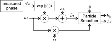
In addition to the experiments, we carried out simulations to isolate the impact of phase noise and to investigate the phase noise limited performance of our system. A block diagram of the simulation model is shown in figure 2. As only additive noise and laser phase noise are included in the simulation model, it does indeed correspond to a phase noise limited system. The phase noise sequence used in the simulations is taken from a measurement with the experimental setup. Thus, the performance of the simulation model corresponds to the best that could be achieved with the laser sources in use.

The experimental and simulation results for $M=4$ and $M=2$ are shown in figures 3 and 4 respectively. A typical value of $p_{r}$ is $0.5$ jouguet2013 but in principle it could also be lower. Bob’s phase estimation should only use the transmitted symbols that are revealed anyway. Therefore, we investigate our system for a low $p_{r}$ of $0.05$. Additionally, we investigate the cases $p_{r}=0$ and $p_{r}=1$. While $p_{r}=1$ represents an upper bound for the performance of phase estimation, $p_{r}=0$ shows the achievable performance without symbol revelation. Also, the case $p_{r}=0$ could be interesting for other fields than CV-QKD where symbol revelation is not possible.

With $p_{r}=0$, the receiver sensitvity in the experimental system is $\mathrm{SNR}_{b,\mathrm{min}}=$-6.9\text{\,}\mathrm{dB}$$. This is in very good agreement with the simulation, where the signal demodulation completely fails at an $\mathrm{SNR}_{b}$ of $-8\text{\,}\mathrm{dB}$. Thus, despite the narrow linewidth fiber lasers, the receiver sensitivity is limited by phase noise. In terms of received optical power, at least $1.5\text{\,}\mathrm{ph}\text{/}\mathrm{sym}$ would be required. This is too high for the discrete phase modulation scheme with $M=4$, where the transmitted optical power should usually be lower than $0.5\text{\,}\mathrm{ph}\text{/}\mathrm{sym}$ leverrier2011. However, even a small revelation probability of $p_{r}=$0.05$$ is sufficient to enable successful signal demodulation down to at least an $\mathrm{SNR}_{b}$ of $-19.1\text{\,}\mathrm{dB}$. In the experiment, the SNR was not decreased further because the receiver calibration was not accurate enough to allow for a reliable evaluation of $\mathrm{SNR}_{b}$ and the excess noise in that regime. The experimentally confirmed receiver sensitivity of $\mathrm{SNR}_{b,\mathrm{min}}<$-19.1\text{\,}\mathrm{dB}$$ is sufficient for CV-QKD over $26\text{\,}\mathrm{km}$ and more. In the simulation results, it can be seen that the carrier phase estimation can be successful down to an $\mathrm{SNR}_{b}$ of $-35\text{\,}\mathrm{dB}$. However, there is already an increased probability of failure above $-35\text{\,}\mathrm{dB}$ as can be seen in the simulations for $M=2$ shown in figure 4, where the minimum $\mathrm{SNR}_{b}$ was $-33\text{\,}\mathrm{dB}$. Therefore, we take this higher value as the receiver sensitivity.

The simulations show the phase noise limited performance. At an $\mathrm{SNR}_{b}$ of $10\text{\,}\mathrm{dB}$, there is no difference in the resulting excess noise between different probabilities of revelation. Apparently, in that case the uncertainty about the carrier phase is not increased by the discrete phase modulation. This is the SNR regime of classical communications where symbol error rates are low and the modulation could also be canceled effectively before carrier phase estimation. In the quantum regime of $\mathrm{SNR}_{b}<$0\text{\,}\mathrm{dB}$$, the modulation clearly affects the carrier phase estimation and hence the excess noise. With $p_{r}=1$, $\xi_{b}^{\prime}$ exhibits a constant slope of about $3\text{\,}\mathrm{dB}$ per decade. This is the result of a decreasing quantum signal power decreasing the excess noise while at the same time decreasing the SNR increases the carrier phase uncertainty which induces additional excess noise. With $p_{r}=0$, in the regime of $\mathrm{SNR}_{b}<$5\text{\,}\mathrm{dB}$$, there is a net increase of $\xi_{b}^{\prime}$ with decreasing $\mathrm{SNR}_{b}$ until the demodulation fails completely. Interestingly, for $p_{r}=0.05$, there is not much value of the revelation around $\mathrm{SNR}_{b}\approx$0\text{\,}\mathrm{dB}$$. In this regime, the unrevealed symbols still provide significant information about the carrier phase. But in the regime of $\mathrm{SNR}_{b}<$-8\text{\,}\mathrm{dB}$$, the slope of $\xi_{b}^{\prime}$ approaches the one of the case $p_{r}=1$. In this regime, the revealed symbols provide more information about the carrier phase than the unrevealed ones and the difference between $p_{r}=1$ and $p_{r}=0.05$ can be interpreted as a difference of the effective symbol rate. Due to this, there is a relatively constant excess noise penalty of about a factor of $9$ in the $\mathrm{SNR}_{b}$ regime between $-10\text{\,}\mathrm{dB}$ and $-26\text{\,}\mathrm{dB}$. Below an $\mathrm{SNR}_{b}$ of $-26\text{\,}\mathrm{dB}$, the slope is flattened.

Looking at the experimental results for the excess noise, we observe a much higher level than in the simulations. Also, there is a proportional relation between $\hat{\xi}_{b}^{\prime}$ and $\mathrm{SNR}_{b}$ that slightly flattens below an $\mathrm{SNR}_{b}$ of $-7\text{\,}\mathrm{dB}$. This confirms that the excess noise mainly originates from signal distortions. The signal to distortion ratio can be quantified for $\mathrm{SNR}_{b}=$7.1\text{\,}\mathrm{dB}$$ as $P_{\mathrm{Q}}/\xi_{b}\approx$31.82$$, which is relatively low and could be improved by optimizing the equalization concept.

For $M=2$, the results are shown in figure 4. The main difference to $M=4$ is that the receiver sensitivity for the case $p_{r}=0$ is much lower. In the simulations it was $\mathrm{SNR}_{b,\mathrm{min}}=$-17\text{\,}\mathrm{dB}$$ and in the experiment $\mathrm{SNR}_{b,\mathrm{min}}=$-13.2\text{\,}\mathrm{dB}$$ compared to the $-6.9\text{\,}\mathrm{dB}$ for $M=4$. The difference between experiment and simulations seems quite large. However, there is still a significant probability of successful demodulation below these values in the experiments and simulations. This indicates that the probability of failure increases less steep with decreasing $\mathrm{SNR}_{b}$ as in the case of $M=4$. With $p_{r}=$0.05$$, the transition to relying only on the revealed symbols for phase estimation is much wider for $M=2$ compared to $M=4$. Even at $\mathrm{SNR}_{b}=$-30\text{\,}\mathrm{dB}$$, the excess noise is slightly lower with $M=2$ compared to $M=4$. However, there is no significant difference between these two cases in terms of experimental excess noise which is dominated by other signal distortions.

In order to address the question of whether or not the performance of the investigated system with a real LO and without pilots is sufficient for CV-QKD, we calculated asymptotic secret key rates. The calculations are based on the well established security proofs leverrier2010 and leverrier2011. These assume a linear Gaussian channel and are therefore not fully general. Recently, a security proof that does not incorporate these assumptions has been presented ghorai2019. However, the question of how to get rid of the linear Gaussian assumption is still under discussion.

We optimized the transmitted optical power with respect to a maximum key rate. For this, we used the polynomial fits for the excess noise in the case of $p_{r}=$0.05$$ that are plotted in the figures 3 and 4. An additional constraint of the optimization was that $\mathrm{SNR}_{b}$ is not allowed to be lower than in the experiments and simulations respectively and also not allowed to be lower than the receiver sensitivity. The measured receiver efficiency $\hat{\eta}$, the electronic noise ratio $\hat{\varepsilon}_{\mathrm{el}}$ as well as the fiber length are also included in the secret key rate calculations. The reconciliation efficiency is assumed to be $95\text{\,}\mathrm{\%}$.

The resulting secret key rates for $p_{r}=$0.05$$ are shown in figure 5. As a reference, the case of zero excess noise is also plotted. The simulation corresponds to the case of the excess noise being dominated by carrier phase uncertainty. In this case, distances of up to $72\text{\,}\mathrm{km}$ could be achieved with $M=4$ and $32\text{\,}\mathrm{km}$ with $M=2$. This shows that laser phase noise is not an insurmountable obstacle for designing a CV-QKD system with a real LO and without pilots. Even for the experimental system, where the excess noise is much higher due to other signal distortions, CV-QKD could be performed successfully with $M=4$ at a key rate of $5.7\text{\times}{10}^{-4}\text{\,}\mathrm{bit}\text{/}\mathrm{sym}$ over the experimental distance of $26\text{\,}\mathrm{km}$. With $M=2$, the experimental performance is not sufficient for CV-QKD. The worse performance of $M=2$ is due to stricter requirements regarding the transmitted power and excess noise leverrier2011. The experimental key rate can be improved towards the simulation by reducing signal distortions in the experiment. This can be achieved by improving the equalization concept of the system. To achieve the long distances that are possible as shown by the simulations, the receiver calibration should be improved. We expect that this can be achieved by reducing the time difference between calibration and quantum signal transmission in order to mitigate fluctuations of the receiver noise and LO power. If the system is optimized such that it is limited by phase noise, the parameter $p_{r}$ can be increased which directly reduces the excess noise for even higher key rates and longer distances. Also, increasing $p_{r}$ can enable the use of lasers with stronger phase noise while keeping the achievable distance.

To conclude, we investigated a fiber-based quantum communication system for CV-QKD that employs a real LO and works without any pilot tones. As Bob’s clock and LO are free running, he relies only on the modulated quantum signal itself to perform carrier phase estimation and timing recovery. Except for the fact that the signal is attenuated before it is transmitted, the physical implementation is identical to classical coherent systems. For the first time it could be demonstrated experimentally, that such a system can be feasible for CV-QKD. An important factor to achieve this is the particle smoother that is used for carrier phase estimation, which is optimized using Monte Carlo Markov chain methods. Based on the experimental results, the achievable key rate over a distance of $26\text{\,}\mathrm{km}$ is $5.7\text{\times}{10}^{-4}\text{\,}\mathrm{bit}\text{/}\mathrm{sym}$ corresponding to $9.2\text{\,}\mathrm{Mbit}\text{/}\mathrm{s}$. The simulation results indicate that this performance can even be largely improved. Possible ways to achieve this is by reducing other signal distortions than phase noise and by improving the receiver calibration. The achieved results are an important milestone for CV-QKD. Also, the achieved receiver sensitivities without symbol revelation ($p_{r}=0$) of $-6.9\text{\,}\mathrm{dB}$ for $M=4$ and $-13.2\text{\,}\mathrm{dB}$ for $M=2$ have, to our knowledge, never been reached before. Therefore, the novel techniques are also beneficial in other coherent systems where the SNR can be extremely low, such as optical satellite communications.