Quantum Plasmonic Immunoassay Sensing
Abstract
Plasmon-polaritons are among the most promising candidates for next generation optical sensors due to their ability to support extremely confined electromagnetic fields and empower strong coupling of light and matter. Here we propose quantum plasmonic immunoassay sensing as an innovative scheme, which embeds immunoassay sensing with recently demonstrated room temperature strong coupling in nanoplasmonic cavities. In our protocol, the antibody-antigen-antibody complex is chemically linked with a quantum emitter label. Placing the quantum-emitter enhanced antibody-antigen-antibody complexes inside or close to a nanoplasmonic (hemisphere dimer) cavity facilitates strong coupling between the plasmon-polaritons and the emitter label resulting in signature Rabi splitting. Through rigorous statistical analysis of multiple analytes randomly distributed on the substrate in extensive realistic computational experiments, we demonstrate a drastic enhancement of the sensitivity up to nearly 1500% compared to conventional shifting-type plasmonic sensors. Most importantly and in stark contrast to classical sensing, we achieve in the strong-coupling (quantum) sensing regime an enhanced sensitivity that is no longer dependent on the concentration of antibody-antigen-antibody complexes – down to the single-analyte limit. The quantum plasmonic immunoassay scheme thus not only leads to the development of plasmonic bio-sensing for single molecules but also opens up new pathways towards room-temperature quantum sensing enabled by biomolecular inspired protocols linked with quantum nanoplasmonics.
keywords
Nano-plasmonics, Strong-coupling, Bio-sensing, Immunoassay, Rabi-splitting1 Introduction
Plasmon-polaritons facilitate strong light-matter interaction by squeezing light into subwavelength volumes Maier 2007; Novotny and Hecht 2012. It triggers a wide range of nanoscale phenomena and applications such as integrated nano-circuits Xiong et al. 2013; Bermúdez-Ureña et al. 2015, nanolasers Bergman and Stockman 2003; Hill and Gather 2014; Pickering et al. 2014, ultraslow (broadband) waves Tsakmakidis et al. 2017, surface-enhanced Raman spectroscopy Ding et al. 2016, and plasmonic sensing Arroyo and Kukura 2016. Many efforts have been focused on the Purcell enhancement of spontaneous emission rate Purcell 1946, however, remaining in the weak coupling regime. In this weak-coupling regime, the energy decays fast and before a significant coherent interchange between plasmon-polaritons and emitters takes place. Recent experiments and computational simulations have successfully demonstrated Väkeväinen et al. 2013; Antosiewicz et al. 2014; Zengin et al. 2015; Chikkaraddy et al. 2016; Liu et al. 2017; Groß et al. 2018 and explained Kongsuwan et al. 2018 room-temperature strong light-matter coupling, offering the possibilities for quantum information processing at room temperature and in ambient environment Altewischer et al. 2002; Gonzalez-Tudela et al. 2011; Tame et al. 2013; Xu et al. 2018. Indeed, the field of nanoplasmonic strong coupling is rapidly evolving from emitter-ensemble Väkeväinen et al. 2013; Antosiewicz et al. 2014; Zengin et al. 2015 toward single-emitter strong coupling Chikkaraddy et al. 2016; Liu et al. 2017; Groß et al. 2018 which is of key importance in many quantum technologies Birnbaum et al. 2005; Kasprzak et al. 2010; Vasa and Lienau 2017, heralding various functional devices operating at the single photon level Chang et al. 2007; Hensen et al. 2017; Tiecke et al. 2014; Sun et al. 2018. Here, we link ensemble-, few- and single-emitter nanoplasmonic strong coupling with immunoassay sensing.
An immunoassay is a biochemical test that measures the presence or concentration of specific molecules in a solution using antibodies Wild 2005. A molecule detected in an immunoassay is often referred to as an “analyte”. Clearly, the ultimate goal of immunoassay sensing is to detect a single analyte enabling, for example, diagnosis of early-stage cancer. However, due to the size mismatch between typical analytes (typically 100 nm) and the optical wavelength (400700 nm), single-analyte sensing has remained elusive. Hence, most immunoassays rely on specific detectable labels that are chemically linked with antibodies. In a plasmonic immunoassay, the sensing signal can be further enhanced as plasmonic structures can efficiently squeeze light into tiny, sub-wavelength volumes that are comparable to the size of the analyte. Various types of labels that are chemically linked to antibodies, can further enhance the sensing signals via their interactions with plasmon-polaritons. For example, a dielectric label has been used to induce changes in the refractive index, shifting the plasmonic resonance Wang et al. 2011; Krishnan et al. 2011. In addition to the refractive index change, a metallic nanoparticle label can also induce hybridization of plasmonic modes with the surrounding structure Lyon et al. 1998; Hong and Hall 2012; Szunerits et al. 2014; Yang et al. 2016. Fluorophores have also been proposed as sensing labels in surface-plasmon field-enhanced fluorescence spectroscopy Liebermann and Knoll 2000; Wang et al. 2009; Wang et al. 2016 where the photoluminescence is enhanced due to the Purcell effect of the plasmonic resonance. In spite of this significant enhancement through a suitable nanoplasmonic environment, the sensing process – interactions between various types of labels and plasmon-polaritons in modern plasmonic immunoassays – have to date not yet explored the strong-coupling quantum regime.
In this study, we propose a new scheme that embeds and utilizes strong coupling between quantum emitter label(s) and plasmon-polaritons to achieve a drastically enhanced sensitivity, down to a single-analyte quantum plasmonic immunoassay. It is from this single-analyte perspective that we shall in the following start our discussion before subsequently moving to the experimentally more common multi-analyte (ensemble) case. In each case, the ultra-sensitivity is achieved via the characteristic spectral signature of Rabi splitting which is effectively a bi-directional shift. Compared to label-free plasmonic sensing, the presence of quantum emitter labels provides a sensitivity enhancement of a factor of 14.2, while solitary dielectric and gold nanoparticle (AuNP) labels give sensitivity enhancements of only 2.62 and 2.73, respectively.
Our statistical studies on multi-analyte detection demonstrate that the proposed protocol also works well in the weak coupling regime (just as conventional plasmonic sensors do) when the emitter labels are displaced from the plasmonic hotspot. In the case of multiple randomly positioned analytes, the optical spectrum of the composite system is not necessarily associated with a Lorentzian line-shape and we consequently introduce a figure of merit (FoM) as the integral of the spectral changes. The immunoassay-FoM in the weak coupling (or classical) regime decreases from 0.226 to 0.093 with decreasing number of analytes. In contrast, the immunoassay-FoM in the strong coupling (or quantum) regime remains approximately constant (around 0.360), independent of the concentration of emitter labels. Indeed, it retains this value also for a single emitter label.

Results and discussion
Strong-Coupling Immunoassay
The principle and set-up of our proposed quantum plasmonic immunoassay sensing protocol are schematically illustrated in Fig. 1a. It functionally involves four main parts: (i) a plasmonic nano-dimer cavity (here formed by two gold hemispheres), (ii) an antigen as the “analyte” to be detected, (iii) a sensing label (which is used to enhance the sensitivity in either a classical or quantum regime), and (iv) two antibodies which are paired with the target antigen and chemically linked with the sensing label, respectively. For our strong-coupling immunoassay, we use a quantum emitter (such as a quantum dot) as the sensing label, and the term “strong-coupling" refers to the strong coupling between the emitter label and the plasmonic field in the cavity. The sensing label can, however, also be a dielectric or plasmonic nanoparticle resulting in a conventional (classical) plasmonic immunoassay. We generally assume that immunoassay takes place in a liquid environment, such as water or serum. A critical layer of dielectric spacer is introduced between the plasmonic hemispheres and the substrate to provide the opportunity to adjust the vertical position of the hotspot, , to coincide with the sensing label. Figure 1b shows the side-view for a representative strong-coupling immunoassay system. The dimer gap between the two nanoplasmonic hemispheres is denoted as . All the simulations are performed on the basis of a 3D full-wave spatio-temporal simulation method based on a finite-difference time-domain (FDTD) scheme (Lumerical Solutions Inc.; see Methods).
To appreciate the functionality of the various components, let us first establish the optical response of an empty hemisphere dimer. Figure 1c shows the normalized electric field distribution of a dimer with a gap = 2 nm resulting in a plasmonic resonance at 1.89 eV. The characteristic plasmonic hotspot is clearly seen inside the nanogap, with a field enhancement by a factor of 195 at the gap center. It is this enhancement that generally forms the foundation for plasmonic sensing with high sensitivity in an ambient environment. Now to demonstrate the sensitivity of the strong-coupling immunoassay, Fig. 1d compares its extinction spectrum (solid red curve) to the spectra of label-free (dotted black curve), dielectric-labeled (dashed blue curve) and AuNP-labeled (dash-dotted green curve) immunoassays. In all cases of the study, we use the same gold hemisphere dimer and dielectric spacers but vary the different sensing complexes inside the gap.
In the label-free case, we place only one antibody and one antigen inside the gap, adjusting the height of the antibody such that the antigen is close to the plasmonic hotspot, while in the case of the labeled complexes we adjust the geometry such that the label resides close to the plasmonic hotspot. The dielectric label itself is approximated as a simple nano-cylinder (radius: 1 nm and height: 2 nm) with a refractive index of 1.8, whereas the AuNP label is modeled as a gold nano-sphere (with the diameter of 1 nm). We use a full-wave spatio-temporal Maxwell-Bloch model Kongsuwan et al. 2018 to take into account the energy exchange dynamics between the two-level quantum emitters (linewidth of 26 meV) and the plasmonic field, revealing the dynamics in both weak- and strong-coupling regimes. Compared to conventional sensing protocols that have a characteristic shift of the optical resonance, the strong-coupling immunoassay exhibits the characteristic signature of strong coupling, , the two Rabi peaks, as indicated in Fig. 1d. This is in effect a bi-directional shift with higher sensitivity than those of conventional immunoassays. In the following, we will investigate and present the principles of the strong-coupling immunoassay.
Anti-Crossing of Strong Coupling
For an emitter coupled with a plasmonic resonance, the system-Hamiltonian can be written as Baranov et al. 2017:
| (1) |
where and are the resonances of the emitter and the plasmon-polaritons, and and are their decay rates, respectively. Then the coupled system has two new eigen-frequencies expressed as Baranov et al. 2017:
| (2) |
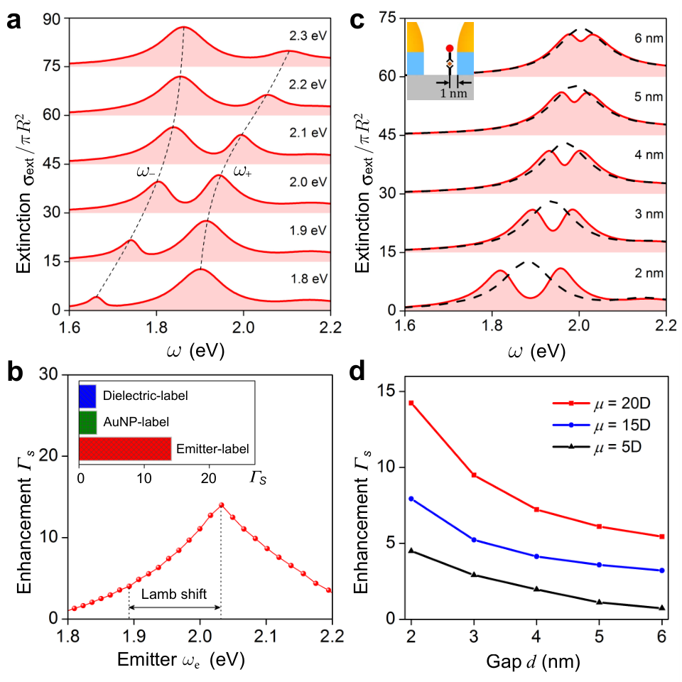
where is the detuning which can be adjusted to control the optical responses of the coupled system. When the coupling rate is slower than the decay processes , the coupled system is in the weak coupling regime where the emitter’s emission rate is enhanced by plasmon-polaritons due to the Purcell effect. The system reaches the strong-coupling regime when the coupling exceeds the decay , at which the emitter and the plasmon-polaritons become hybridized and coherently exchange energy. In this regime, the hybridized system frequencies and reveal a clear anti-crossing pattern as we sweep the emitter resonance across the plasmonic resonance . As shown in Fig. 2a, the numerically calculated extinction spectra of coupled system show clearly two branches, when the hemisphere dimer with = 1.89 eV is coupled to different emitter with = 1.8-2.3 eV. We shall in the following use this type of spectral signature to characterize the performance of our strong-coupling immunoassay scheme.
Sensitivity
For conventional shifting-type plasmonic sensors (, the dotted black, dashed blue, and dash-dotted green curves in Fig. 1d), the (sensing) sensitivity is generally defined as the ratio of the change in sensor output (, resonance shift ) relative to the change in the quantity to be measured (, concentration of the analyte ) Homola 2008. However, while is a good measure in the case of appreciable analyte concentrations, measuring concentrations is clearly no longer well-applicable in the context of few- or single-analyte detection. We thus adopt the number of analytes (where 1, 2, 3, …) as quantifying descriptor to define sensitivity as:
| (3) |
to be used here to characterize the shifting-type plasmonic sensors for few- or single-analyte detection, an example of which is indicated by the blue arrow in Fig. 1d. On the other hand, for the strong-coupling immunoassay (splitting-type), there are double shifts toward both directions, as illustrated by the red arrows in Fig. 1d. The measurable frequency splitting between the peaks can be (analytically) expressed as:
| (4) |
Compared to the original resonance detuning , the system response is modified by due to the coupling between the emitter(s) and the plasmon-polaritons. Therefore, we define the sensitivity of our strong-coupling (or splitting-type) immunoassay as:
| (5) |
We note that in principle, when the emitter and plasmons are on resonance (), the frequency difference corresponds to the Rabi splitting, and the sensitivity should thus reach its maximum. For the off-resonance cases (), we expect a drop of the sensitivity . In the context of single-analyte detection (), the sensitivity is purely relevant to the resonance shift for shifting-type sensors () or to the resonance splitting for strong-coupling sensors ().
To directly compare various different types of sensors, we normalize the sensitivities to that of the label-free sensor, denoting the normalized sensitivity as , which characterizes the sensitivity enhancement induced by the sensing labels. The inset of Fig. 2b shows the sensitivity enhancement (extracted from the spectra in Fig. 1d) for different labels. We observe a clear enhancement of 15-fold () in strong-coupling immunoassay sensing, making it a competitive candidate for next-generation sensors. We also extract the sensitivity enhancement for the strong-coupling immunoassay from Fig. 2a, which is dependent on the emitter resonance as shown in Fig. 2b. Clearly, there exists an optimal as we sweep the emitter resonance. However, due to the optical Lamb shift experienced by the emitter label (see Section S1 in Supporting Information), this optimal does not occur at = 1.89 eV when the emitter and the plasmon-polaritons are on resonance. This suggests that the ideal emitter label should be slightly detuned from the plasmonic cavity resonance in order to maximize the sensitivity. In practice, however, it might be more convenient to design a suitably detuned plasmonic cavity for any pre-selected emitter label in a plasmonic immunoassay system.
When seeking to optimize the sensitivity of our immunoassay system we can vary geometrical parameters such as the gap width or choose a particular emitter label with a characteristic transition dipole moment . Determining the dependence of the sensitivity enhancement on the dimer gap we first focus on the spectral response of empty hemisphere dimers of variable gap width = 2–6 nm as shown in Fig. 2c (black dashed lines). As the dimer gap decreases, the plasmonic resonance is red-shifted, thus the emitter resonance must be tuned for each gap according to the similar optimization procedure illustrated in Fig. 2b. The corresponding extinction spectra with optimized and maximized are obtained for various dimer gaps as shown in Fig. 2c (red solid lines). For smaller dimer gap , the Rabi splitting of the coupled system becomes more prominent, indicating a stronger coupling strength between the emitter and the plasmon-polaritons. Similarly, we extract the sensitivity enhancement from these extinction spectra. As shown in Fig. 2d, increases drastically as the dimer gap decreases. Note that, for this gap size study, the emitter is displaced from the gap center and stays 1 nm away from one of the hemisphere’s surface, as illustrated in the inset of Fig. 2c. This position is optimized to provide the highest sensitivity enhancement (see Section S2 in Supporting Information). If we now vary the transition dipole moment , Fig. 2d shows that as expected, increases for larger . Typical emitters that are used for strong coupling include methylene blue ( 1.878 eV, D) Chikkaraddy et al. 2016; Patil et al. 2000, J-aggregates ( 2.145 eV, D) Zengin et al. 2015; Liu et al. 2017, and rhodamine ( 1.741 eV, D) Delysse et al. 1998; Wuestner et al. 2010. Moreover, some III-V quantum dots (, InAs and GaAs) Khitrova et al. 2006 and defects in two-dimensional materials (, WS and graphene) Sie 2018 have also been used, with their ranging from 10D to 100D. In this context, we should point out that the previously mentioned 15-fold sensitivity enhancement is achieved using a conservative value of D. Of course, we may anticipate even higher sensitivity enhancement with a larger dipole moment . Besides, this study also clearly confirms the preferred choice of dimers with small gaps for improved sensitivity.

Strong-Coupling Photoluminescence Spectra
In typical strong coupling experiments, the extinction spectrum is usually obtained by measuring the amount of radiation transmitted through the coupled system as a function of the wavelength of the incident light. However, the “splitting” feature manifested in the extinction spectrum is not a sufficient condition to determine the occurrence of strong coupling between one or more emitters and plasmon-polaritons. In fact, such splitting may also originate from absorption or interference Laussy et al. 2009. To rigorously confirm that we are, indeed, achieving strong coupling, we calculate the photoluminescence (PL) spectrum of the emitter in our strong-coupling immunoassay system by deriving a master equation within the framework of cavity quantum electrodynamics (cQED) (see Section S4 in Supporting Information). To represent the Hamiltonian of the coupled system, we adopt the quasi-normal mode (QNM) method and obtain the coupling strength and decay rates from the Purcell factors of QNMs (see Sections S3-S4 in Supporting Information). Experimentally, this PL spectrum can be measured by exciting the emitter with a pump laser and collecting the luminescence from the coupled system Melnikau et al. 2016; Groß et al. 2018. Fundamentally, both extinction and PL spectra describe the dynamic interactions of the coupled system. However, they originate from different processes: extinction spectra reflect stimulated absorption and emission processes of the coupled system (whose signal interferes with the background excitation light), whereas the PL reveals the spontaneous emission of the coupled system without the background excitation light.
Figure 3a shows in direct comparison both the PL and extinction spectra for strong-coupling immunoassay systems with = 2–6 nm. It is for a (large) gap size of = 6 nm, where the discrepancy between the PL and extinction spectra becomes most noticeable. Although the extinction spectrum has two splitting resonance peaks, the single peak in the PL spectrum indicates that the emitter and plasmon-polaritons are, in fact, in the weak coupling regime. The splitting peaks in the extinction spectrum emerge simply due to the interference between the emitter and plasmon-polaritons Laussy et al. 2009. As the gap size decreases ( 4 nm), both the PL and extinction spectra have two split peaks, unambiguously indicating the strong coupling between emitter and plasmon-polaritons. The occurrence of strong coupling is perhaps most strongly manifested in the dynamics of the polarization of the quantum emitter and its dependence on different gap sizes. Figures 3b and 3c show normalized by the incident field amplitude in linear and logarithmic presentations. In Fig. 3b, we can see a second wave packet for a small gap = 2 nm as a direct evidence of the revival of the emitter Rempe et al. 1987 which occurs thanks to its interaction with the plasmon-polaritons in the strong coupling regime. Such dynamics then emerges in the logarithmic presentation as ripples for small dimer gaps ( 5 nm).
The PL spectrum and time-dependent analysis reveal more underlying physics than just the extinction spectrum. However, due to complex energy transfer and recombination processes of the vibrational and defect states Melnikau et al. 2016 involved, it is experimentally also more challenging to observe Rabi splitting in the PL spectrum than in the extinction spectrum. It is not less challenging to calculate within a cQED framework the combined PL spectrum of an ensemble of analyte-emitter complexes. As the emitters at different locations experience , different amounts of optical Lamb shifts and Purcell enhancements, the emitters cannot be considered indistinguishable. Indeed, even if they are of the same type the retardations and interactions between different emitters must also be considered. Hence, the computation within the cQED framework would increase exponentially with the emitter number. When in the following analyzing sensing properties of a spatially (randomly) distributed ensemble of analytes we will model the spatio-temporal strong-coupling dynamics in terms of a full-wave Maxwell-Bloch approach Kongsuwan et al. 2018 adapted to our immunoassay configuration. Adopting an experimentally relevant set-up we will focus on the extinction spectrum which is of course accurate enough in terms of spectroscopically characterizing the sensing performance through comparisons before and after the adsorption of analyte-emitter complexes.
Statistics and Figure of Merit (FoM)
In a typical immunoassay set-up, there will be a number of analytes dissolved in a liquid. To realistically model experiments with this set-up in our in silico experiment (for details regarding the simulation set-up see Section S5 in Supporting Information), we now focus on an ensemble of analyte-complexes (each including a quantum emitter), which are randomly distributed in the vicinity of the nano-dimer and subject to an average surface density. This random distribution reflects the consequence of many complex physical and chemical processes such as transport and molecular inter-interaction which indeed merit consideration in future studies. As illustrated in Fig. 4a, most of the analyte-complexes will in a typical situation be randomly distributed around the two nano-dimer hemispheres, but there is also the chance to find one or more of the complexes in the gap between the hemispheres. Indeed, with increasing surface density of analyte-emitter complexes the probability to find an analyte-emitter in the center of the dimer gap increases. This reflects the fact that just like in an in vitro experiment, even with all the quantum emitters resonance at = 2.03 eV, every emitter experiences a different nano-plasmonic environment and thus exhibits different degrees of the optical Lamb shifts.

We perform a statistical study on the case of multiple analyte-emitter complexes, and obtain the extinction spectra of 30 samples for each surface density (see Figs. S5-S10 in Supporting Information). From the large simulation sample space, we select several representative spectra and classify them into two groups, as shown in Fig. 4b. For the first group (top row of Fig. 4b), the spectra (solid blue curves) exhibit a major peak shifted from the original plasmonic resonance (dashed black curves), accompanied by some minor peaks, especially when the surface density increases. For these spectra with one major peak, the interaction between emitter label and plasmon-polaritons is still in the weak coupling regime, , none of the emitters is in the center of the dimer gap. In contrast, for the second group (bottom row of Fig. 4b), the spectra (solid red curves) have two major peaks, each of which may possess their own splitting sub-peaks. This “splitting” indicates that the strong coupling occurs because of a “random” emitter located in the center of the dimer gap. Accordingly, we define the first group (or the shifting-type) and the second group (or the splitting-type) as the classical and quantum sensors, respectively.
It is worth noting that, as the surface density of analyte-emitter complexes increases, the spectrum in quantum regime no longer consists of well-defined (or Lorentz-shape) peaks at distinct frequencies. Therefore, we define a figure of merit (FoM) to characterize the performance of multi-analyte detection as:
| (6) |
in which we integrate the change of extinction cross-section over the whole spectral range and normalize it to the extinction cross-section of the empty dimer. This FoM effectively quantifies the optical change before and after the adsorption of the analyte-emitter complexes. The statistics on FoM for different surface densities of analyte-emitter complexes are summarized in Fig. 4c, where the hollow triangles represent the samples that we have studied (30 samples for each surface density). The solid lines show the average FoMs of classical and quantum sensors at each surface density, and the dotted line at FoM = 0.3 is used to differentiate classical and quantum regimes. The histogram of FoMs for all the studied samples can also be found in Fig. S11 in Supporting Information.
From Fig. 4c, we observe that for a large surface density of analyte-emitter complexes, there is no clear boundary between the FoMs of classical and quantum regimes. As the surface density decreases, FoM in the classical regime drops drastically from 0.226 to 0.093. However, the FoM in quantum regime remains almost constant ( 0.360), because it dominantly results from the single emitter located at the plasmonic hotspot. This proves that, toward single-analyte detection, the strong-coupling immunoassay protocol unambiguously outperforms the shifting-type sensors. We also note an increased fluctuation in FoM for quantum sensors with increasing surface density. A larger number of quantum emitters randomly scattered near the plasmonic hotspot introduces uncertainty in the coupling strength due to complex many-body interactions between the emitters and plasmon-polaritons.
So far, we have presented a simple nanostructure with a few-nm gap to demonstrate splitting-type sensing. Such a small size of this gap is clearly not without practical challenges. For example, fabrication of a nanogap must be sufficiently pristine in order to accommodate an antibody, and the steric effect could be significant in such a small gap and prevent a complex from binding at the narrowest (optimal) location. However, our analysis with many different random distributions shows that an analyte does not necessarily have to be at this most narrow point to achieve quantum plasmonic immunoassay sensing. In fact, strong coupling could be achieved at a larger gap size using a quantum emitter with larger dipole moment. Alternatively, an open cavity using a plasmonic nanocube Liu et al. 2017 could also provide sufficient field confinement at its corners and is certainly more accessible for biomolecules. Another alternative could be detecting a small antigen without a much larger antibody by using artificial proteins to capture the antigen between a plasmonic dimer Chevrel et al. 2008; Yim et al. 2008; Gurunatha et al. 2016.
Conclusion
In summary, we have proposed and demonstrated the effectiveness of an innovative immunoassay sensing protocol by employing quantum emitters as sensing labels of anitibody-antigen-antibody complexes which in (hemispherical) nanoplasmonic open cavities facilitate room-temperature strong coupling. The proposed splitting-type sensing approach demonstrates a nearly 15-fold sensitivity enhancement over conventional shifting-type label-free plasmonic sensors. The underlying mechanism of the gigantic sensitivity enhancement is attributed to the splitting of the original resonance, which is equivalent to a bi-directional resonance shifting. Using quantum emitter labels with realistically strong transition dipole moments , extensive numerical experiments with varying nanogap widths allow us to suggest that nanogaps below 5 nm would be ideal systems for strong coupling conditions and also suggest slight detuning from the plasmonic resonance. Moreover, using randomly distributed multi-analyte systems with variable random analyte distributions as realistic model systems for biological experiments reveals that our proposed immunoassay protocol is able to perform both classical and quantum sensing. A new figure of merit (FoM) is defined to quantify the spectral difference before and after the adsorption of the analyte-emitter complexes in this multi-analyte study. We show that with decreasing concentration of analytes, the FoM degrades rapidly for classical sensors, yet quantum sensors are able to maintain a stable, concentration-independent FoM. This demonstrates a genuine potential for experiments based on our quantum plasmonic immunoassay sensing protocol to finally reach the single-analyte detection limit. While the current proposal engages a quantum phenomenon (, strong coupling with a quantum emitter) to detect a classical object (, antigen) the approach can conceivably be extended to detect a quantum object such as an electronic spin in nanodiamonds Maze et al. 2008; Taylor et al. 2008; Doherty et al. 2013. This opens up a new pathway toward plasmonics-enabled room-temperature quantum sensing Fan et al. 2015; Lee et al. 2016; Degen et al. 2017.
Methods
To obtain the extinction cross-sections and polarization responses, we perform finite-difference time-domain simulations using a commercial software from Lumerical version 8.18.1298. The permittivity of gold is modeled from the experimental results from Johnson and Christy Johnson and Christy 1972. The nanostructure is illuminated by the total-field scattered-field (TFSF) source with background refractive index . The simulation domain size is 1 m 1 m 1 m. We utilize the conformal meshing scheme between dielectric interfaces, but not on metal interfaces, with a maximum step size of 30 nm in all directions. While finer meshes of 0.25 nm and 0.5 nm are used on analyte-complexes and the Au hemisphere dimer, respectively.
The dynamics of the (two-level) quantum emitter label(s) is modelled self-consistently with the full-wave spatio-temporal dynamics of the optical field on the basis of an FDTD scheme. An individual emitter is (for simplicity) assumed as embedded within a single Yee cell which interacts with the electromagnetic fields through its polarization density in the Maxwell equation . For an emitter with transition frequency and transition dipole moment 20D (unless otherwise stated) oriented along unit vector , its polarization is calculated by the Maxwell-Bloch equations Boyd 2003; Kongsuwan et al. 2018:
| (7) |
| (8) |
| (9) |
where = 0.25 nm is the mesh size at the emitter’s position, = 26 meV is the FWHM linewidth, is the relaxation rate, and , , are the diagonal and off-diagonal elements of the density matrix. Note that in our simulations, the total electric field is corrected by the divergent field Schelew et al. 2017:
| (10) |
| (11) |
where is the background permittivity, as the polarization field generated by the emitter is through numerical self-interaction in a Yee-cell grid (unless corrected as done in our simulations) re-inserted into the simulation and thus (erroneously) re-excited.
Author Information
Corresponding Authors
E-mail: wul@ihpc.a-star.edu.sg
E-mail: o.hess@imperial.ac.uk
Author Contributions
N.K.and X.X. contributed equally to this work. N.K. and X.X. performed the simulations and wrote the manuscript. N.K. and J.Y. carried out theoretical derivations. P.B., C.E.P., L.W. and O.H. contributed to data analysis. L.W. and O.H. supervised the entire project. All authors commented on the manuscript.
Note
The authors declare no conflict of interest.
valuation of the optical Lamb shift of an emitter label at different locations. Location of the emitter label in the simulations with different gap size. The theory of Quasinormal modes. Multi-mode Purcell enhancement estimations of plasmonic modes. Statistical study of multi-analyte detection with varying analtye concentrations.
References
- Maier (2007) Maier, S. A. Plasmonics: fundamentals and applications; Springer Science & Business Media, 2007.
- Novotny and Hecht (2012) Novotny, L.; Hecht, B. Principles of nano-optics; Cambridge university press, 2012.
- Xiong et al. (2013) Xiong, X.; Zou, C. L.; Ren, X. F.; Liu, A. P.; Ye, Y. X.; Sun, F.-W.; Guo, G. C. Laser Photonics Rev. 2013, 7, 901–919.
- Bermúdez-Ureña et al. (2015) Bermúdez-Ureña, E.; Gonzalez-Ballestero, C.; Geiselmann, M.; Marty, R.; Radko, I. P.; Holmgaard, T.; Alaverdyan, Y.; Moreno, E.; García-Vidal, F. J.; Bozhevolnyi, S. I., et al. Nat. Commun. 2015, 6, 7883.
- Bergman and Stockman (2003) Bergman, D. J.; Stockman, M. I. Phys. Rev. Lett. 2003, 90, 027402.
- Hill and Gather (2014) Hill, M. T.; Gather, M. C. Nat. Photonics 2014, 8, 908.
- Pickering et al. (2014) Pickering, T.; Hamm, J.; Page, A.; Wuestner, S.; Hess, O. Nat. Commun. 2014, 5.
- Tsakmakidis et al. (2017) Tsakmakidis, K.; Hess, O.; Boyd, R.; Zhang, X. Science 2017, 358.
- Ding et al. (2016) Ding, S.-Y.; Yi, J.; Li, J.-F.; Ren, B.; Wu, D.-Y.; Panneerselvam, R.; Tian, Z.-Q. Nat. Rev. Mater. 2016, 1, 16021.
- Arroyo and Kukura (2016) Arroyo, J. O.; Kukura, P. Nat. Photonics 2016, 10, 11.
- Purcell (1946) Purcell, E. M. Phys. Rev. 1946, 69, 681–681.
- Väkeväinen et al. (2013) Väkeväinen, A.; Moerland, R.; Rekola, H.; Eskelinen, A.-P.; Martikainen, J.-P.; Kim, D.-H.; Törmä, P. Nano Lett. 2013, 14, 1721–1727.
- Antosiewicz et al. (2014) Antosiewicz, T. J.; Apell, S. P.; Shegai, T. ACS Photonics 2014, 1, 454–463.
- Zengin et al. (2015) Zengin, G.; Wersäll, M.; Nilsson, S.; Antosiewicz, T. J.; Käll, M.; Shegai, T. Phys. Rev. Lett. 2015, 114, 157401.
- Chikkaraddy et al. (2016) Chikkaraddy, R.; de Nijs, B.; Benz, F.; Barrow, S. J.; Scherman, O. A.; Rosta, E.; Demetriadou, A.; Fox, P.; Hess, O.; Baumberg, J. J. Nature 2016, 535, 127.
- Liu et al. (2017) Liu, R.; Zhou, Z.-K.; Yu, Y.-C.; Zhang, T.; Wang, H.; Liu, G.; Wei, Y.; Chen, H.; Wang, X.-H. Phys. Rev. Lett. 2017, 118, 237401.
- Groß et al. (2018) Groß, H.; Hamm, J. M.; Tufarelli, T.; Hess, O.; Hecht, B. Sci. Adv. 2018, 4.
- Kongsuwan et al. (2018) Kongsuwan, N.; Demetriadou, A.; Chikkaraddy, R.; Benz, F.; Turek, V. A.; Keyser, U. F.; Baumberg, J. J.; Hess, O. ACS Photonics 2018, 5, 186–191.
- Altewischer et al. (2002) Altewischer, E.; Van Exter, M.; Woerdman, J. Nature 2002, 418, 304.
- Gonzalez-Tudela et al. (2011) Gonzalez-Tudela, A.; Martin-Cano, D.; Moreno, E.; Martin-Moreno, L.; Tejedor, C.; Garcia-Vidal, F. J. Phys. Rev. Lett. 2011, 106, 020501.
- Tame et al. (2013) Tame, M. S.; McEnery, K.; Özdemir, Ş.; Lee, J.; Maier, S.; Kim, M. Nat. Phys. 2013, 9, 329.
- Xu et al. (2018) Xu, D.; Xiong, X.; Wu, L.; Ren, X.-F.; Png, C. E.; Guo, G.-C.; Gong, Q.; Xiao, Y.-F. Adv. Opt. Photonics 2018, 10, 703–756.
- Birnbaum et al. (2005) Birnbaum, K. M.; Boca, A.; Miller, R.; Boozer, A. D.; Northup, T. E.; Kimble, H. J. Nature 2005, 436, 87.
- Kasprzak et al. (2010) Kasprzak, J.; Reitzenstein, S.; Muljarov, E. A.; Kistner, C.; Schneider, C.; Strauss, M.; Höfling, S.; Forchel, A.; Langbein, W. Nat. Mater. 2010, 9, 304.
- Vasa and Lienau (2017) Vasa, P.; Lienau, C. ACS Photonics 2017, 5, 2–23.
- Chang et al. (2007) Chang, D. E.; Sørensen, A. S.; Demler, E. A.; Lukin, M. D. Nat. Phys. 2007, 3, 807.
- Hensen et al. (2017) Hensen, M.; Heilpern, T.; Gray, S. K.; Pfeiffer, W. ACS Photonics 2017, 5, 240–248.
- Tiecke et al. (2014) Tiecke, T.; Thompson, J. D.; de Leon, N. P.; Liu, L. R.; Vuletić, V.; Lukin, M. D. Nature 2014, 508, 241.
- Sun et al. (2018) Sun, S.; Kim, H.; Luo, Z.; Solomon, G. S.; Waks, E. Science 2018, 361, 57–60.
- Wild (2005) Wild, D. The immunoassay handbook; Elsevier, 2005.
- Wang et al. (2011) Wang, Y.; Dostalek, J.; Knoll, W. Anal. Chem. 2011, 83, 6202–6207.
- Krishnan et al. (2011) Krishnan, S.; Mani, V.; Wasalathanthri, D.; Kumar, C. V.; Rusling, J. F. Angew. Chem., Int. Ed. 2011, 50, 1175–1178.
- Lyon et al. (1998) Lyon, L. A.; Musick, M. D.; Natan, M. J. Anal. Chem. 1998, 70, 5177–5183.
- Hong and Hall (2012) Hong, X.; Hall, E. A. Analyst 2012, 137, 4712–4719.
- Szunerits et al. (2014) Szunerits, S.; Spadavecchia, J.; Boukherroub, R. Rev. Anal. Chem. 2014, 33, 153–164.
- Yang et al. (2016) Yang, C.-T.; Wu, L.; Liu, X.; Tran, N. T.; Bai, P.; Liedberg, B.; Wang, Y.; Thierry, B. Anal. Chem. 2016, 88, 11924–11930.
- Liebermann and Knoll (2000) Liebermann, T.; Knoll, W. Colloids Surf., A 2000, 171, 115–130.
- Wang et al. (2009) Wang, Y.; Brunsen, A.; Jonas, U.; Dostalek, J.; Knoll, W. Anal. Chem. 2009, 81, 9625–9632.
- Wang et al. (2016) Wang, Y.; Wu, L.; Wong, T. I.; Bauch, M.; Zhang, Q.; Zhang, J.; Liu, X.; Zhou, X.; Bai, P.; Dostalek, J., et al. Nanoscale 2016, 8, 8008–8016.
- Baranov et al. (2017) Baranov, D. G.; Wersall, M.; Cuadra, J.; Antosiewicz, T. J.; Shegai, T. ACS Photonics 2017, 5, 24–42.
- Homola (2008) Homola, J. Chem. Rev. 2008, 108, 462–493.
- Patil et al. (2000) Patil, K.; Pawar, R.; Talap, P. Phys. Chem. Chem. Phys. 2000, 2, 4313–4317.
- Delysse et al. (1998) Delysse, S.; Nunzi, J.-M.; Scala-Valero, C. Appl. Phys. B: Lasers Opt. 1998, 66, 439–444.
- Wuestner et al. (2010) Wuestner, S.; Pusch, A.; Tsakmakidis, K. L.; Hamm, J. M.; Hess, O. Phys. Rev. Lett. 2010, 105, 127401.
- Khitrova et al. (2006) Khitrova, G.; Gibbs, H.; Kira, M.; Koch, S. W.; Scherer, A. Nat. Phys. 2006, 2, 81.
- Sie (2018) Sie, E. J. Coherent Light-Matter Interactions in Monolayer Transition-Metal Dichalcogenides; Springer, 2018; pp 37–57.
- Laussy et al. (2009) Laussy, F. P.; del Valle, E.; Tejedor, C. Phys. Rev. B 2009, 79, 235325.
- Melnikau et al. (2016) Melnikau, D.; Esteban, R.; Savateeva, D.; Sánchez-Iglesias, A.; Grzelczak, M.; Schmidt, M. K.; Liz-Marzán, L. M.; Aizpurua, J.; Rakovich, Y. P. J. Phys. Chem. Lett. 2016, 7, 354–362.
- Rempe et al. (1987) Rempe, G.; Walther, H.; Klein, N. Phys. Rev. Lett. 1987, 58, 353.
- Chevrel et al. (2008) Chevrel, A.; Urvoas, A.; de la Sierra-Gallay, I. L.; Aumont-Nicaise, M.; Moutel, S.; Desmadril, M.; Perez, F.; Gautreau, A.; van Tilbeurgh, H.; Minard, P., et al. Biosci. Rep. 2015, 35, e00223.
- Yim et al. (2008) Yim, T. J.; Wang, Y.; Zhang, X. Nanotechnology 2008, 19, 435605.
- Gurunatha et al. (2016) Gurunatha, K. L.; Fournier, A. C.; Urvoas, A.; Valerio-Lepiniec, M.; Marchi, V.; Minard, P.; Dujardin, E. ACS Nano 2016, 10, 3176–3185.
- Maze et al. (2008) Maze, J.; Stanwix, P.; Hodges, J.; Hong, S.; Taylor, J.; Cappellaro, P.; Jiang, L.; Dutt, M. G.; Togan, E.; Zibrov, A., et al. Nature 2008, 455, 644.
- Taylor et al. (2008) Taylor, J.; Cappellaro, P.; Childress, L.; Jiang, L.; Budker, D.; Hemmer, P.; Yacoby, A.; Walsworth, R.; Lukin, M. Nat. Phys. 2008, 4, 810.
- Doherty et al. (2013) Doherty, M. W.; Manson, N. B.; Delaney, P.; Jelezko, F.; Wrachtrup, J.; Hollenberg, L. C. Phys. Rep. 2013, 528, 1–45.
- Fan et al. (2015) Fan, W.; Lawrie, B. J.; Pooser, R. C. Phys. Rev. A 2015, 92, 053812.
- Lee et al. (2016) Lee, C.; Dieleman, F.; Lee, J.; Rockstuhl, C.; Maier, S. A.; Tame, M. ACS Photonics 2016, 3, 992–999.
- Degen et al. (2017) Degen, C. L.; Reinhard, F.; Cappellaro, P. Rev. Mod. Phys. 2017, 89, 035002.
- Johnson and Christy (1972) Johnson, P. B.; Christy, R. W. Phys. Rev. B 1972, 6, 4370–4379.
- Boyd (2003) Boyd, R. W. Nonlinear optics; Elsevier, 2003.
- Schelew et al. (2017) Schelew, E.; Ge, R. C.; Hughes, S.; Pond, J.; Young, J. F. Phys. Rev. A 2017, 95, 063853.