Extending the Davis–Kahan theorem for comparing eigenvectors of two symmetric matrices II: Computation and ApplicationsPubID: pubid:

Let $\mathbb{V}_{n,r}$ denote the Stiefel manifold of $n\times r$ matrices with orthonormal columns. Let $\Phi,\Psi\in\mathbb{R}^{n\times n}$ be symmetric matrices with eigenvalues $\phi_{1}\leq\phi_{2}\leq\ldots\leq\phi_{n}$ and $\psi_{1}\leq\psi_{2}\leq\ldots\leq\psi_{n}$ and corresponding eigenvectors $\{w_{1},w_{2},\ldots,w_{n}\}$ and $\{v_{1},v_{2},\ldots,v_{n}\}$, respectively. For $j\geq 0,r\geq 1,$ let the matrices holding the eigenvectors corresponding to $r$ consecutive eigenvalues of each matrix be denoted by $W_{j}=[w_{j+1},\ldots,w_{j+r}]\in\mathbb{V}_{n,r}$ and $V_{j}=[v_{j+1},\ldots,v_{j+r}]\in\mathbb{V}_{n,r},$ the columns of which span the spaces $\mathcal{W}_{j}$ and $\mathcal{V}_{j},$ respectively. Under the stated conditions, it was shown in Paper I that there exists a $Q\in O(r)$ such that

where $O(r)$ is the group of $r\times r$ orthogonal matrices, $c_{n,r}=\sqrt{2\min(r,n-r)},$ $p(\cdot)$ is a polynomial matrix transformation and $\delta_{i},i\in\{1,2\}$ are different values of the DK interval separation parameter corresponding to the two different DK interval choices. The usual or standard DK bounds follow by taking $p(\Phi)=\Phi$ in the second inequality. In Paper I we saw that the first norm is directly related to the metric $\rho_{1}(\mathcal{W}_{j},\mathcal{V}_{j})=\inf_{R\in O(r)}\|W_{j}-V_{j}R\|_{F},$ and the second relates to the metric $\rho_{2}(\mathcal{W}_{j},\mathcal{V}_{j})=\left\|W_{j}W_{j}^{T}\left(I-V_{j}V_{j}^{T}\right)\right\|_{2}.$

In this paper we focus on affine matrix transformations $f(\Phi)=c_{1}\Phi+c_{0}I,\,\,(c_{1},c_{0}\in\mathbb{R})$ of one of the matrices under comparison (arbitrarily, $\Phi$). So we set $p(\cdot)=f(\cdot)$ and for $j\geq 0,r\geq 1,$ from Paper I, the two DK interval choices take the form $S_{1}=[a,b],S_{2}=\mathbb{R}\backslash(a-\delta,b+\delta),$ with

The index sets ${\cal A}_{1}$ and ${\cal A}_{2}$ are given in Paper I.

A main purpose of this paper is to solve the problem of optimizing the bound on the right-side of (II-A) when $p(\cdot)=f(\cdot),$ i.e., minimize

subject to the associated constraints given in Paper I. For an affine transformation, Constraints 2 of Paper I must be applied (Constraints 1 are subsumed). Constraints 2 take the form:

1. A

   In the case of interval choice (2), let the transformation parameters of $f(\cdot)$ be chosen such that, for given $j\geq 0,r\geq 1$,

   	$\displaystyle\delta_{1}$	$\displaystyle>0,$		(5)
   	$\displaystyle a_{1}-\psi_{j+1}$	$\displaystyle<\delta_{1},$		(6)
   	$\displaystyle\psi_{j+r}-b_{1}$	$\displaystyle<\delta_{1}.$		(7)

2. B

   For interval choice (3), let the transformation parameters of $f(\cdot)$ be chosen such that, for given $j\geq 0,r\geq 1$,

   	$\displaystyle\delta_{2}$	$\displaystyle>0,$		(8)
   	$\displaystyle a_{2}-\min_{i\in\{j+1,\ldots,j+r\}}f(\phi_{i})$	$\displaystyle<\delta_{2},$		(9)
   	$\displaystyle\max_{i\in\{j+1,\ldots,j+r\}}f(\phi_{i})-b_{2}$	$\displaystyle<\delta_{2}.$		(10)

Also as pointed out in Paper I, in addition to the two DK interval choices which give $\delta_{1},\delta_{2}$ in (4), there are also the possibilities $c_{1}>0$ and $c_{1}<0$ in the affine transform. So there are four different possible values for the DK interval separation $\delta,$ which are,

Here we show that the optimization subproblem (15) and its related subproblems can be efficiently solved using fractional programming theory.

Ratio optimization problems are commonly called fractional programs [9]. Hence, the optimization problem (15) of choosing the affine transformation parameters $(c_{1},c_{0})\in\mathbb{R}^{+}\times\mathbb{R}$ resulting in a minimal bound is a fractional program. We now describe the properties of fractional programs and their solutions. Then we transform (15) to fit the standard class of concave-convex fractional programs and discuss the implementation of its solution.

Firstly, we formally define fractional programs.

In [9], concave-convex fractional programs are referred to as concave fractional programs. An excellent overview of concave-convex fractional programs is given in [13], with a focus on wireless communication.

When discussing the solution of concave-convex fractional programs the concept of equivalence of optimization problems is essential.

Furthermore, we make use of the standard definition of the feasible set of an optimization problem.

Subproblem (15) can be transformed to fall into the class of concave-convex fractional programs. As pointed out in [21],

Using (18) we find that solving (15) is equivalent to solving,

The bound value is found by transforming the solution of (19) according to (18).

We now demonstrate that the subproblems such as (19), are concave-convex fractional programs.

Several general approaches to solving concave-convex fractional programs are presented in [13] and in [25] fractional programming in the context of multiple-ratio problems is discussed.

In Section IV-D, we discuss the parameter-free approach where an equivalent convex problem is obtained through transformation of the optimization parameters; the transformation used is commonly referred to as the Charnes–Cooper transformation. This transformed problem only needs to be solved once. In [5] the Charnes–Cooper transformation is used in the optimization of the energy spectral efficiency of a communication network and in [18] the authors show that the maximum likelihood estimate of the steering direction of a signal for radar detection can be found by utilising the Charnes–Cooper transformation of a fractional programming problem.

In Section IV-E, we treat the parametric approach which introduces an additional parameter $\lambda$ to obtain an equivalent problem, which is not jointly convex in $(c_{1},c_{0})$ and $\lambda$. The equivalent problem, is however, convex in $(c_{1},c_{0})$ and monotone in $\lambda$. Therefore, we iteratively solve the convex problem for $(c_{1},c_{0})$ for a fixed $\lambda$ and update $\lambda$ using a Newton-Raphson step. This algorithm is credited to Dinkelbach [6]. In [27] minimization of the system outage probability in a communication network using Dinkelbach’s algorithm is discussed, using a closed form solution to the problem at each iteration.

For computational reasons we mainly utilise the parameter-free approach, i.e., the Charnes–Cooper transformation. This follows advice in [22] and [23], who state that the iterative solution via Dinkelbach’s algorithm is only to be preferred over the single Charnes–Cooper transformed problem, if the solution via Dinkelbach exploits the structure of the numerator and denominator of the fractional program which the Charnes–Cooper solution does not. For instance for quadratic fractional programs – fractional programs with a quadratic numerator and denominator and affine constraints – Dinkelbach’s algorithm solves a quadratic program at every iteration, while the Charnes–Cooper transformation yields a concave problem. Therefore, if not many Dinkelbach iterations are necessary for convergence, then Dinkelbach’s algorithm is to be preferred over the Charnes–Cooper approach for quadratic fractional programs. We find that for our problem (15) both the Charnes–Cooper transformation and Dinkelbach’s algorithm solve convex or concave problems. Therefore, we prefer the Charnes–Cooper solution method. However, most importantly, the results of the two different approaches agree in our simulations, as would be anticipated from [13] who showed that the optimality conditions of the two approaches are equivalent, so in theory the results should indeed not vary.

Charnes and Cooper [4] proposed a variable transform for linear fractional programs – fractional programs with an affine numerator and denominator and linear constraints. Schaible [20] generalised the transformation to concave-convex fractional programs. [13] give a good recent summary of the transformation of concave-convex fractional problems. For the transformation of (19), appropriate transformation parameters are:

Let

Transforming (19) using the parameters in (IV-D) we obtain the following convex optimization problem:

In the original proposal of the transformation for linear fractional programs [4] the equality constraint $\left\|y_{1}\Phi+y_{2}I-t\Psi\right\|_{2}=1$ was used. This constraint cannot be placed on concave-convex fractional problems, since convex optimization problems can only have linear equality constraints [2, p. 191]. It is proved in [20] that for concave-convex fractional programs the constraints $\left\|y_{1}\Phi+y_{2}I-t\Psi\right\|_{2}=1$ and $\left\|y_{1}\Phi+y_{2}I-t\Psi\right\|_{2}\leq 1$ are equivalent. Therefore, we work with the relaxed constraint $\left\|y_{1}\Phi+y_{2}I-t\Psi\right\|_{2}\leq 1$.

Note that (21) is not a linear program since the constraint $\left\|y_{1}\Phi+y_{2}I-t\Psi\right\|_{2}\leq 1$ contains a non-linear function of the parameters. The constraint is however convex; therefore, (21) is a convex optimization problem.

We implement the 4 subproblems using the cvx package in MATLAB [10, 11]. cvx does not accept strict inequalities. We therefore solve relaxed subproblems, where the strict inequalities are relaxed to include their boundaries, and then check whether the obtained solutions satisfy the strict inequalities. We have found this approach to work extremely well in practice with no convergence issues.

Dinkelbach’s algorithm was proposed in [6]. Equivalent to (19) is the problem

[6] state that the algorithm can be initialised at a feasible point $(c_{1},c_{0})$, which is chosen such that the corresponding $\lambda=g_{1}(c_{1},c_{0})/g_{2}(c_{1},c_{0})$ is positive, or at $\lambda=0$. When we initialise at $\lambda=0$ then any feasible set of transformation parameters $(c_{1},c_{0})$ can be chosen for the initialisation. Therefore, we choose to always initialise at $\lambda=0$ and $(c_{1},c_{0})$ to be equal to their respective optima from the Charnes–Cooper algorithm in the corresponding subproblem.

As with the Charnes–Cooper implementation we utilise relaxed subproblems, where the strict inequality constraints are relaxed to include their boundaries. Then we check and report if any of the strict inequality constraints in the Dinkelbach implementation are violated. We have found the solution of Dinkelbach’s algorithm to agree with the solution of the Charnes–Cooper algorithm in all cases we tested.

Dinkelbach’s scheme was extremely useful for checking that our implementation of the Charnes–Cooper scheme was correct, but it offered no advantages over the latter, and was much slower.

The stochastic blockmodel, which is widely used in the networks literature [12, 16, 17], allows us to encode a block structure in a random graph via different probabilities of edges within and between node-blocks. The definition and parametrisation below is adapted from [17].

Hence, the parameters of the stochastic blockmodel are $M\in\{0,1\}^{n\times K}$ and $P\in[0,1]^{K\times K},$ where the number of nodes $n\in\mathbb{N}$ and the number of clusters $K\in\mathbb{N}$ are implicitly defined via the dimensions of $M.$ We simulate graphs from this model by fixing these parameters and then sampling edges from Bernoulli trials. The Bernoulli parameter of the trial corresponding to the edge connecting $v_{i}$ to $v_{j}$ is given by entry $(i,j)$ of the matrix $B_{A}=MPM^{T}$.

Since our results apply only to symmetric matrices, we work with undirected graphs, which can be derived from a stochastic blockmodel by sampling the upper triangular half of the adjacency matrix from the stochastic blockmodel and then equating the lower triangular part of the adjacency matrix to the transpose of the upper triangle.

Throughout this section we take the matrix of edge probabilities to be composed of only two values. On the diagonal we have $p_{w}$ encoding the probability of edges within the different blocks to be the same for all blocks. Off-diagonal we have $p_{b}$ to encode the probability of edges between nodes in different blocks. For example, for $K=3,$ $P$ takes the form:

For affine transforms, from (II-A) and (4) the bound of interest is the right-hand-side of

where $\delta_{i}$ equals $\delta_{1,+},\delta_{1,-},\delta_{2,+}$ or $\delta_{2,-},$ from Equations (11)-(14), which generate the four different optimization subproblems of the form (19).

In this section we divide all bound values and attained values by $c_{n,r},$ i.e., we consider instead

This rescaling has the advantage that, independent of $n$ and $r,$ our bound values are on the same relative scale. Furthermore, the trivial bound derived in Proposition 1 corresponds to the upper bound of 1 in all plots, rather than the value $c_{n,r},$ which would vary across the different simulations.

In what follows, (scaled) attained distance in the metric $\rho_{1}(\mathcal{W}_{j},\mathcal{V}_{j})$ refers to the quantity $c_{n,r}^{-1}\inf_{R\in O(r)}\|W-VR\|_{F}$ and (scaled) attained distance in the metric $\rho_{2}(\mathcal{W}_{j},\mathcal{V}_{j})$ refers to $\left\|W_{j}W_{j}^{T}-(I-V_{j}V_{j}^{T})\right\|_{2}.$ (For the first of these we recall from Paper I that, when calculating distances, finding the matrix $Q$ for which the infimum is attained can be avoided by the use of canonical angles.)

In this section we calculate the bound on the distance of the spaces spanned by the eigenvectors of the graph shift operator matrices. Recall that the largest eigenvalues of the adjacency matrix correspond to the smallest eigenvalues of the Laplacians. Hence, in two of the three presented comparisons we will compare spaces spanned by eigenvectors corresponding to eigenvalues on opposing ends of the eigenvalue spectrum. Therefore, in the majority of cases presented in this section the standard DK Theorem does not apply, while bound values can be obtained via our extended DK Theorem.

Throughout this section we consider stochastic blockmodels with $K=3,$ where every block is composed of equally many nodes. The parameters identifying the compared eigenvectors are $j=1$ and $r=2$. This choice of $j$ and $r$ is motivated by the fact that the first eigenvector of the Laplacian matrices is a constant vector and is therefore not informative in the recovery of the blocks in the stochastic blockmodel. Hence, we are comparing spaces spanned by eigenvectors corresponding to the second and third largest eigenvalue of the adjacency matrix to those corresponding to the second and third smallest eigenvalues of the two graph Laplacians.

In Figs. 1 (a) and (b) we plot the bound and attained values arising from the comparison of the spaces spanned by eigenvectors of the three graph shift operator matrices against the degree extremes of the corresponding graphs. We simulated $n_{sim}=25$ stochastic blockmodels with equal parameters $n=300,K=3,(p_{b},p_{w})=(0.1,0.6).$

In Fig. 1(a) we observe that the bound grows with a growing degree extreme difference for the comparisons of $L$ with $A$ and $L_{sym}$, while the bound remains relatively constant across different degree extremes when $A$ and $L_{sym}$ are compared. The bound values for comparisons of $L$ with $A$ and $L_{sym}$ are very close, differing only by very small amounts. The bound arising from the comparison of $A$ and $L_{sym}$ attains much lower values than the bound values arising from the other two comparisons. Hence, using an affine transformation we are able to obtain a very small bound on the difference of spaces spanned by the eigenvectors of $A$ and $L_{sym}$, which suggests that they are very close. Not only are they close to each other, they also produce extremely similar bounds on the space spanned by the eigenvectors when individually compared to the eigenvectors of $L.$

In Fig. 1(b) we observe that the attained distances of the three comparisons remain rather constant across the different degree extreme differences.

The results in Fig. 1 show that for the comparison of $A$ and $L_{sym}$ an affine transformation is sufficient to remove the dependence of the bound value on the degree extreme difference. In contrast the much higher bounds for the comparison of the eigenvectors of $L$ with $A$ and $L_{sym}$ still depends on the degree extreme difference and the affine transformation was not sufficient to remove this dependence.

In Fig. 2, we observe the effect of a growing number of network nodes $n$ on our bound. For each value of $n\in\{30,120,210,300\}$ we simulated $25$ stochastic blockmodels with equal parameters $K=3,(p_{b},p_{w})=(0.1,0.9).$ In all plots the four values of $n$ are displayed on the $x$-axis. The first column of plots in Fig. 2 displays boxplots of the bound values of the three possible pairwise comparisons, while the second and third columns display boxplots of the optimal affine transformation parameters $c_{1}$ and $c_{0},$ respectively. The rows of plots show the comparison of spaces spanned by eigenvectors of $A$ and $L,$ (first), $L$ and $L_{sym},$ (second) and $A$ and $L_{sym},$ (third). Just the 25 samples from each stochastic blockmodel parametrisation were sufficient to reveal general trends in the 9 plots.

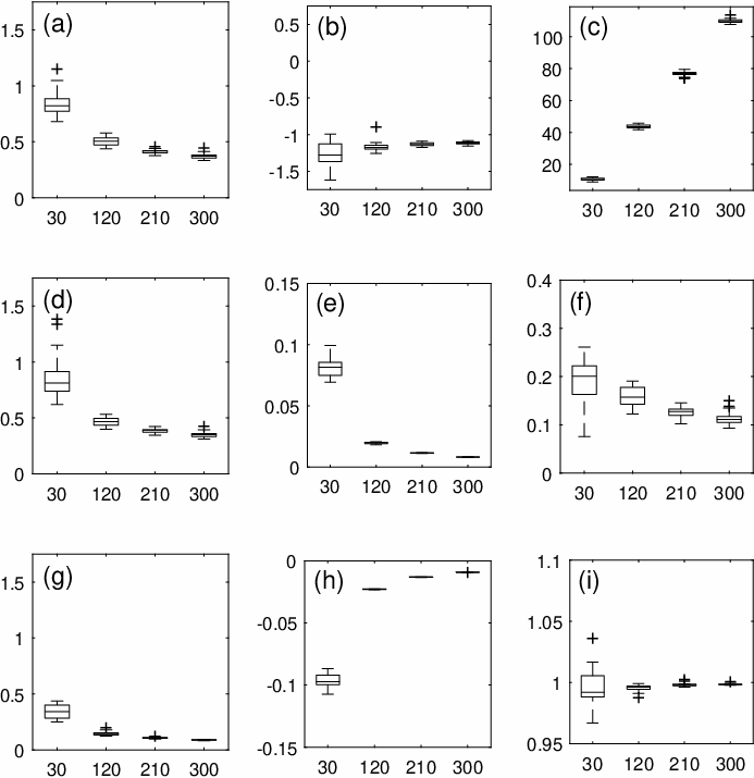
From Fig. 2 (a), (d) and (g) we immediately see that the bound values decrease as the number of nodes in the stochastic blockmodels grows indicating that as $n$ grows the differences between the spaces spanned by the eigenvectors of the graph shift operator matrices decrease. From Fig. 2 (b), (c), (e), (f), (h) and (i) we observe the majority of optimal affine transformation parameters depend on $n.$ For the comparison of $A$ and $L,$ in Fig. 2(c), we find the optimal additive parameter $c_{0}$ to grow from roughly 10 for $n=30$ to roughly 110 for $n=300,$ while the multiplicative parameter in Fig. 2(b) remains almost constant for all values of $n$. Comparison of the Laplacian matrices $L$ and $L_{sym},$ shows both transformation parameters vary slightly with $n,$ (Figs. 2(e) and (f)). Finally, comparison of $A$ and $L_{sym},$ shows the additive parameter $c_{0}$ to remain mostly constant with changing $n$ (Fig. 2(i)) while the multiplicative parameter $c_{1}$ grows with $n$ (Fig. 2(h)). The magnitude by which the transformation parameters change as $n$ grows is clearly quite variable.

We were unable to run the simulation displayed in Fig. 2 beyond $n=300$ within reasonable computation time. The times for the simulations with the four different values of $n$ were, $3,21,118$ and $472$ minutes, respectively. For each value of $n,$ 300 convex optimization problems were solved since each bound on the three possible graph shift operator matrix comparisons was calculated for 25 different stochastic blockmodels per value of $n$ and calculation of each bound involves the solution of 4 different convex optimization subproblems.

In this section we compare (i) spaces spanned by eigenvectors of the graph shift operator matrices to (ii) spaces spanned by eigenvectors of their corresponding generating matrices in the stochastic blockmodel $B_{A}=MPM^{T}-\mathrm{diag}(MPM^{T}),B_{L}=\mathrm{diag}(B_{A}\mathbf{1}_{n})-B_{A}$ and $B_{L_{sym}}=\mathrm{diag}(B_{A}\mathbf{1}_{n})^{-1/2}B_{L}\mathrm{diag}(B_{A}\mathbf{1}_{n})^{-1/2}.$ (Here $\mathbf{1}_{n}$ is a column vector of ones with $n$ entries and the term $-\mathrm{diag}(MPM^{T})$ in the calculation of $B_{A}$ ensures that our stochastic blockmodels do not have self-loops.) It is natural to compare the spaces spanned by these eigenvectors, since consistency and rate of convergence of different methods, based on the eigenvectors of the graph shift operator matrices in a stochastic blockmodel setting, can be demonstrated [3, 7, 19].

In Figs. 3(a) and (b) the bound and attained values from the comparison of the spaces spanned by the eigenvectors of the three graph shift operator matrices to the eigenvectors of their respective generating matrices are plotted against the degree extremes of the corresponding graphs. In the adjacency matrix comparison, the eigenvectors corresponding to the three largest eigenvalues are compared, while for the Laplacians we concern ourselves with the eigenvectors corresponding to the three smallest eigenvalues. $25$ realisations of a stochastic blockmodel with parameters $n=210,K=3,(p_{b},p_{w})=(0.1,0.9)$ were simulated. In this comparison we included the first eigenvector of the matrices under comparison, i.e., we chose $j=0$ and $r=3.$

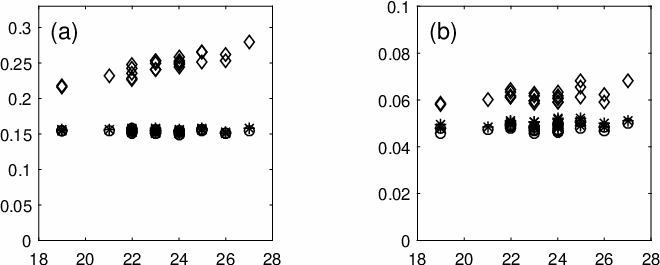
We see in Fig. 3 that the ordering in magnitude of the attained values is reflected in the bound values, with the bounds on the unnormalised Laplacian comparison $(L,B_{L})$ taking the largest values. We see that both the attained and the bound values in the comparison of the spaces spanned by eigenvectors of $L$ and $B_{L}$ seem to grow with growing degree extreme difference, which is not the case for the comparisons involving $A$ and $L_{sym}.$

In Fig. 4 we observe the effect of a growing number of network nodes $n$ on our bound. For each value of $n\in\{30,120,210,300\}$ we simulated $25$ stochastic blockmodels with parameters $K=3,(p_{b},p_{w})=(0.1,0.8).$ The transformation parameters are roughly centred around the parameters of the identity transformation, $f(x)=x,$ i.e., $c_{1}=1$ and $c_{0}=0$. Interestingly, the variance of the additive parameter $c_{0}$ seems to be increasing with increasing $n$ for the comparison $(L,B_{L}).$ For all other displayed values in Fig. 4 we find the variance of the observed values to decrease as the number of nodes in the network grows. As the number of nodes, $n,$ in the stochastic blockmodel grows, the bound values of all three comparisons decrease.

For the spaces spanned by the leading eigenvectors of the graph shift operator matrices compared to their corresponding generating matrices, Fig. 5 shows the usual DK bounds (Theorem 3 of Paper I), our sharpened bounds (Theorem 5 of Paper I and (24)) and the attained values; all were standarized. Here $25$ realisations of a stochastic blockmodel with parameters $n=30,K=3,(p_{b},p_{w})=(0.1,0.6)$ were generated. In all three comparisons, our sharpened bound values improve on the usual DK bound values. In the case of the unnormalised Laplacian several of the usual DK bound values are greater than 1, therefore, even the trivial bound value of 1 (see Proposition 1 and Section V-B) is tighter than the usual DK bound. In contrast, our bound produces values consistently lower than 1.

In addition to the attained distances of the spaces spanned by the eigenvectors in the metric $\rho_{1}(\mathcal{W}_{0},\mathcal{V}_{0}),$ we have shown the distance in the metric $\rho_{2}(\mathcal{W}_{0},\mathcal{V}_{0})$ in Fig. 5, which is discussed in Paper I. As expected from Lemma 2 and Theorem 5 in paper I, we find the attained values $\rho_{2}(\mathcal{W}_{0},\mathcal{V}_{0})$ to fall between the distances in the metric $\rho_{1}(\mathcal{W}_{0},\mathcal{V}_{0})$ and our sharpened DK values. Of particular interest are the values attained in simulation number 10 in Fig. 5(b), where we find the distance of the spaces spanned by the eigenvectors to come very close to 1 in the metric $\rho_{2}(\mathcal{W}_{0},\mathcal{V}_{0})$ and our sharpened bound to be very close to tight in this instance.

Our final example of the application of our sharpened DK bound is in the setting of Principal Component Analysis (PCA). Consider $N\in\mathbb{N}$ independent, identically distributed samples $\{X_{i}\}$ from a multivariate normal distribution of dimension $p\in\mathbb{N},$ with mean $\mathbf{0}$ and covariance matrix $\Sigma.$ Then let $X$ be the $p\times N$ matrix with columns $X_{i}$ with $i\in\{1,\ldots,N\}$. We denote the sample covariance matrix by $\hat{\Sigma}=XX^{T}/N.$ When a low dimensional structure truly generates the covariance matrix, PCA is the correct tool to recover this low dimensional space. The standard PCA algorithm maps the data into the space spanned by the $r$ eigenvectors corresponding to the largest eigenvalues of $\hat{\Sigma}.$ In this setting it is of interest to study the convergence of the space spanned by these leading $r$ eigenvectors of $\hat{\Sigma}$ to the leading eigenvectors spanning the true low dimensional covariance space of $\Sigma$. Using a so-called spiked covariance model, we will apply our bound to the spaces spanned by eigenvectors corresponding to the largest eigenvalues of $\Sigma$ and $\hat{\Sigma}$.

The spiked covariance model was first introduced by [14], who described a phenomenon in real world data where the largest eigenvalues of the covariance matrix are separated by a large eigengap from the rest of the spectrum. [15] proved consistency of the first $r$ eigenvectors of the estimated sample covariance towards the population covariance in the case of zero mean normally-distributed data and under certain conditions on the growth of the largest eigenvalues with growing dimensions $p$ and $N.$ The spiked covariance model has been found to be implied by the factor model [8, 24, 26], which models a multivariate time series as being driven by a few main factors. The factor model and consequently the spiked covariance model, find application to financial data.

In our parametrisation of the spiked covariance model $r\in\mathbb{N}$ determines the dimension of the low-dimensional latent space in which $\Sigma$ is generated, $M\in\{0,1\}^{p\times r}$ encodes the latent dimension membership (similar to the stochastic blockmodel) and $P\in\mathbb{R}^{r\times r}$ encodes the correlations between latent dimensions. $\Sigma$ has to be a valid covariance matrix, so must be symmetric positive definite. As for the stochastic blockmodels, we chose $P$ to consist of only two values and take the form given in (23). We define the population covariance matrix as,

By building our covariance matrix like this, we get a covariance matrix following the spiked covariance model, where $r$ eigenvalues are significantly larger than the rest of the spectrum ([14, 15]), the latter consisting of eigenvalues all equal to 1, as a result of adding $I$ into the covariance structure.

In Fig. 6(a) we plot our sharpened bound for spaces spanned by the eigenvectors corresponding to the largest 3 eigenvalues of $\Sigma$ and $\hat{\Sigma}$ and in Fig. 6(b) and (c) the corresponding optimal transformation parameters $c_{1}$ and $c_{0}$, respectively. Here $N\in\{10,100,1000\},p=60,(p_{b},p_{w})=(0.2,0.8),j=0,r=3.$ In Fig. 6(a) we see the bound decreases as the sample size $N$ grows. This makes sense: more samples should improve the estimation performance of the sample covariance matrix and therefore the distance of the subspaces spanned by the first three eigenvectors of the sample and population covariance matrices should decrease. For $N=10$ samples we find that in a few cases the bound value 1 is attained. This situation was theoretically discussed in Proposition 1. It is nice to see that we do indeed find the bound to converge to 1 with diverging transformation parameters in the worst case in practice. In plots (b) and (c) we find the transformation parameters to converge to the identity transformation as $N$ grows.

The format of Fig. 7 follows Fig. 6 with the difference that we keep $N$ fixed at 100 and study the behaviour of our bound as $p$ grows, $p\in\{30,210,420\}.$ Interestingly, our bound remains fairly constant for the values of $p$ considered. The transformation parameters hover around the identity transformation $f(x)=x$ with the uncertainty in the additive parameter $c_{0}$ increasing as $p$ increases.

Using $N=100,p=60,(p_{b},p_{w})=(0.4,0.6),j=0,r=3,$ and 25 simulations, Fig. 8 shows that our extended or sharpened DK bounds improve upon the usual DK bounds by roughly a factor of 2. In Proposition 1 it was discussed that bound values above 1 are non-informative. In Fig. 8 we observe our bound to consistently fall below 1, improving on the trivial bound; however, the usual DK bound attains values consistently above 1.

In this Appendix we first work out the limit of bound (15) as either $c_{0}\rightarrow\infty$ or $c_{0}\rightarrow-\infty$ for comparisons with $j=0$. Then we draw parallels to the comparisons involving the last $r$ eigenvectors, i.e., the case where $j=n-r.$

We begin by producing a lower and an upper bound for the cost function in (15). Using the matrix triangle and reverse-triangle inequalities $\big|||A||-||B||\big|\leq||A-B||$ and $||A+B||\leq||A||+||B||$ on the numerator of the cost function, gives

But $\left\|I\right\|_{2}=1$ so henceforth this term will be omitted. Here $\delta$ is any of $\delta_{1,+},\delta_{1,-},\delta_{2,+}$ and $\delta_{2,-}$ corresponding to the four subproblems which need to be solved in the affine case. For $j=0,$ we encounter the issue that $\phi_{0}$ and $\psi_{0}$ are undefined and therefore, as is done in [28, p. 317] we set them equal to $-\infty.$ Then, (11), (12), (13) and (14) take the following form,

In order to work out the limit of the lower and upper bound in (25) as either $c_{0}\rightarrow\infty$ or $c_{0}\rightarrow-\infty$ we use l’Hopital’s rule. For l’Hopital’s rule to apply we require both the numerator and the denominator of the lower and upper bound in (25) to tend to 0 or $\infty$ as either $c_{0}\rightarrow\infty$ or $c_{0}\rightarrow-\infty$. We find that both numerators and their common denominators do indeed tend to $\infty$ as either $c_{0}\rightarrow\infty$ or $c_{0}\rightarrow-\infty$, i.e.,

We start by evaluating the derivative with respect to $c_{0}$ of the numerator of both the lower and upper bound in (25) and of their denominators.

Consider firstly $({\partial}/{\partial c_{0}})\left(\big|\left|c_{0}\right|-\left\|c_{1}\Phi-\Psi\right\|_{2}\big|\right)=\mathrm{sign}\left(\left|c_{0}\right|-\left\|c_{1}\Phi-\Psi\right\|_{2}\right)\mathrm{sign}(c_{0}).$ This derivative is: $1$ for $\left\|c_{1}\Phi-\Psi\right\|_{2}<c_{0};$ $-1$ for $0<c_{0}<\left\|c_{1}\Phi-\Psi\right\|_{2};$ $1$ for $-\left\|c_{1}\Phi-\Psi\right\|_{2}<c_{0}<0,$ and $-1$ for $c_{0}<-\left\|c_{1}\Phi-\Psi\right\|_{2}.$

References

- [1] D. S. Bernstein, Matrix Mathematics: Theory, Facts, and Formulas (2nd. Edition), Princeton, NJ: Princeton University Press, 2009.
- [2] S. Boyd & L. Vandenberghe, Convex optimization, Cambridge, U.K.: Cambridge University Press, 2004.
- [3] J. Cape, M. Tang & C. E. Priebe, “Signal-plus-noise matrix models: eigenvector deviations and fluctuations,” Biometrika, vol. 106, pp. 243 – 250, 2019.
- [4] A. Charnes & W. W. Cooper, “Programming with linear fractional functionals,” Naval Research logistics quarterly, vol. 9, pp. 181 – 186, 1962.
- [5] K. T. K. Cheung & L. Hanzo, “Distributed Energy Spectral Efficiency Optimization for Partial/Full Interference Alignment in Multi-user Multi-relay Multi-cell MIMO Systems,” IEEE Transactions on Signal Processing, vol. 64, pp. 882–896, 2016.
- [6] W. Dinkelbach, “On Nonlinear Fractional Programming,” Management Science, vol. 13, pp. 492–498, 1967.
- [7] J. Eldridge, M. Belkin & Y. Wang, “Unperturbed: spectral analysis beyond Davis–Kahan,” Proceedings of Algorithmic Learning Theory, vol. 83, pp. 321–358, 2018.
- [8] J. Fan, Y. Liao & M. Mincheva, “Large covariance estimation by thresholding principal orthogonal complements,” Journal of the Royal Statistical Society B, vol. 75, pp. 603–680, 2013.
- [9] H. Frenk & S. Schaible, Fractional Programming, In: C. Floudas , P. Pardalos (eds) Encyclopedia of Optimization, Boston, MA: Springer, 2009.
- [10] M. Grant & S. Boyd, CVX: Matlab software for disciplined convex programming, version 2.1, http://cvxr.com/cvx, Accessed: September 2018.
- [11] M. Grant & S. Boyd, Graph implementations for nonsmooth convex programs, In: V. Blondel, S. Boyd, H. Kimura (eds) Recent Advances in Learning and Control, Boston, MA: Springer, 2008.
- [12] P. W. Holland, K. B. Laskey & S. Leinhardt, “Stochastic Blockmodels: First Steps,” Social Networks, vol. 5, pp. 109–137, 1983.
- [13] C. Isheden, Z. Chong, E. Jorswieck & G. Fettweis, “Framework for link-level energy efficiency optimization with informed transmitter,” IEEE Transactions on Wireless Communications, vol. 11, pp. 2946–2957, 2012.
- [14] I. M. Johnstone, “On the distribution of the largest eigenvalue in principal components analysis,” The Annals of Statistics, vol. 29, pp. 295–327, 2001.
- [15] S. Jung & J. S. Marron, “PCA consistency in High Dimension Low Sample Size Context,” The Annals of Statistics, vol. 37, pp. 4104–4130, 2009.
- [16] B. Karrer & M. E. J. Newman, “Stochastic blockmodels and community structure in networks,” Phys. Rev. E, vol. 83, pp. 016107, 2011
- [17] J. Lei & A. Rinaldo, “Consistency of spectral clustering in stochastic block models,” The Annals of Statistics, vol. 43, pp. 215–237, 2015.
- [18] A. De Maio, Y. Huang, D. P. Palomar, S. Zhang & A. Farina, “Fractional QCQP With Applications in ML Steering Direction Estimation for Radar Detection,” IEEE Transactions on Signal Processing, vol. 59, pp. 172–185, 2011.
- [19] K. Rohe, S. Chatterjee & B. Yu, “Spectral clustering and the high-dimensional stochastic blockmodel,” The Annals of Statistics, vol. 39, pp. 1878–1915, 2011.
- [20] S. Schaible, “Parameter-free Convex Equivalent and Dual Programs of Fractional Programming Problems,” Zeitschrift für Operations Research, vol. 18, pp. 187–196, 1974.
- [21] S. Schaible, “Minimization of Ratios,” Journal of optimization theory and applications, vol. 19, pp. 347–352, 1976.
- [22] S. Schaible, “Fractional Programming: Applications and algorithms,” European Journal of Operations Research, vol. 7, pp. 111–120, 1981.
- [23] S. Schaible, “Fractional Programming,” Zeitschrift für Operations Research, vol. 27, pp. 39–54, 1983.
- [24] D. Shen, H. Shen & J. S. Marron, “A general framework for consistency of principal component analysis,” Journal of Machine Learning Research, vol. 17, pp. 1–34, 2016.
- [25] K. Shen & W. Yu, “Fractional Programming for Communication Systems—Part I: Power Control and Beamforming,” IEEE Transactions on Signal Processing, vol. 66, pp. 2616–2630, 2018.
- [26] W. Wang & J. Fan, “Asymptotics of empirical eigenstructure for high dimensional spiked covariance,” The Annals of Statistics, vol. 45, pp. 1342–1374, 2017.
- [27] Y. Ye, Y. Li, Z. Wang, X. Chu & H. Zhang, “Dynamic Asymmetric Power Splitting Scheme for SWIPT-Based Two-Way Multiplicative AF Relaying,” IEEE Signal Processing Letters, vol. 25, pp. 1014–1018, 2018.
- [28] Y. Yu, T. Wang & R. J. Samworth, “A useful variant of the Davis–Kahan theorem for statisticians,” Biometrika, vol. 102, pp. 315–323, 2015.