Bond particle theory for the pseudogap phase of underdoped cuprates

We consider the t-J model on a 2D square lattice with $N$ sites, labeled by indices $i$, $j$ and periodic boundary conditions. The Hamiltonian readsChao; ZhangRice

$\displaystyle H=-\sum_{i,j}\;\sum_{\sigma}t_{i,j}\hat{c}_{i,\sigma}^{\dagger}\hat{c}_{j,\sigma}+J\;\sum_{\langle i,j\rangle}\;{\bf S}_{i}\cdot{\bf S}_{j},$

where $\hat{c}_{i,\sigma}^{\dagger}=c_{i,\sigma}^{\dagger}(1-n_{i\bar{\sigma}})$ ${\bf S}_{i}$ is the operator of electron spin at site $i$ and $\langle i,j\rangle$ denotes a sum over all pairs of nearest neighbors. We assume that the hopping integrals $t_{i,j}$ are different from zero only for nearest ($(1,0)$-like), 2^nd nearest ($(1,1)$-like) and 3^nd nearest ($(2,0)$-like) neighbors, and call the respective hopping integrals $t$, $t^{\prime}$ and $t^{\prime\prime}$. The nearest neighbor $t$ will be taken as the unit of energy.

The basic idea of the calculation is to represent eigenstates of a single dimer by bond bosons (for even electron number) and bond fermions (for odd electron number). We consider a single dimer with the sites labeled $1$ and $2$ and first write down the four states with two electrons, that means the singlet and the triplet. Introducing the matrix $4$-vector $\bm{\gamma}=(\tau_{0},\bm{\tau})$ with $\tau_{0}=1$ and $\bm{\tau}$ the vector of Pauli matrices, the state $4$-vector $\bm{\beta}=(s,\bm{t})$ isSachdevBhatt; Gopalan

$\displaystyle|\bm{\beta}\rangle=\frac{1}{\sqrt{2}}\;\sum_{\sigma,\sigma^{\prime}}\;c_{1,\sigma}^{\dagger}\;(\bm{\gamma}i\tau_{y})_{\sigma,\sigma^{\prime}}\;c_{2,\sigma^{\prime}}^{\dagger}|0\rangle.$

(1)

The four states with a single electron can be classified by their parity and $z$-spinSushkovladder; Sushkov_doped

$\displaystyle|f_{\pm,\sigma}\rangle$

$\displaystyle=$

$\displaystyle\frac{1}{\sqrt{2}}\;(c_{1,\sigma}^{\dagger}\pm c_{2,\sigma}^{\dagger})|0\rangle.$

(2)

The last eigenstate is the empty dimer $|e\rangle=|0\rangle$. If the dimer is in one of the states with two electrons, (1), we consider it as occupied by a boson, created by the operator $4$-vector $(s^{\dagger},{\bf t}^{\dagger})$, whereas a dimer in one of the states (2) is considered as occupied by a fermion, created by $f_{\pm,\sigma}^{\dagger}$. If the dimer is empty we again consider it as occupied by a boson, created by $e^{\dagger}$. The states $|s\rangle$, $|f_{+,\sigma}\rangle$ and $|e\rangle$ are even under the exchange $1\leftrightarrow 2$, whereas $|{\bf t}\rangle$ and $|f_{-,\sigma}\rangle$ are odd. We ascribe positive parity also to the operators $s^{\dagger}$, $f_{+}^{\dagger}$ and $e^{\dagger}$ and negative parity to ${\bf t}^{\dagger}$ and $f_{-}^{\dagger}$. The procedure to transcribe operators for the original t-J model to the representation in terms of bond particles is as follows: since the $9$ states introduced above form a complete basis of the Fock space of a dimer, any operator $O$ acting within that dimer can be expressed as $\sum_{a,b}|a\rangle O_{a,b}\langle b|$, with $O_{a,b}=\langle a|O|b\rangle$. Replacing $|a\rangle\langle b|\rightarrow a^{\dagger}b$ we obtain an operator for the bond particles which has the same matrix elements as long as it is acting in the subspace of states with precisely one bond particle in the dimer. In this way, the representation of the spin operator at site $j\in\{1,2\}$ becomes

	$\displaystyle{\bf S}_{j}$	$\displaystyle\rightarrow$	$\displaystyle\frac{\lambda_{j}}{2}\left(\;s^{\dagger}{\bf t}+{\bf t}^{\dagger}s\;\right)-\frac{i}{2}\;{\bf t}^{\dagger}\times{\bf t}$		(3)
			$\displaystyle\;\;\;\;\;\;\;\;+\frac{1}{4}\;\left(\;{\bf f}_{+}^{\dagger}+\lambda_{j}{\bf f}_{-}^{\dagger}\;\right)\bm{\tau}\left(\;{\bf f}_{+}+\lambda_{j}{\bf f}_{-}\;\right)$

where $\lambda_{j}=(-1)^{j-1}$. Introducing the contravariant spinor ${\bf c}=(\hat{c}_{\uparrow},\hat{c}_{\downarrow})^{T}$ the representation of the electron annihilation operator at site $j$ becomes

	$\displaystyle{\bf c}_{j}$	$\displaystyle\rightarrow$	$\displaystyle:\;\frac{1}{2}\;\left(s\;i\tau_{y}+\lambda_{j}{\bf t}\cdot\bm{\tau}i\tau_{y}\right)\;\left(\;{\bf f}_{+}^{\dagger}-\lambda_{j}{\bf f}_{-}^{\dagger}\;\right)$		(4)
			$\displaystyle\;\;\;\;\;\;\;\;\;\;\;\;\;\;\;\;\;\;\;\;\;\;\;\;\;\;+\frac{1}{\sqrt{2}}\;e^{\dagger}\left(\;{\bf f}_{+}+\lambda_{j}{\bf f}_{-}\;\right)\;:$

where $:\dots:$ denotes normal ordering. As mentioned above, these representations are valid in the subspace of states with precisely one bond particle in the dimer:

$\displaystyle s^{\dagger}s+{\bf t}^{\dagger}\cdot{\bf t}+\sum_{\sigma}\sum_{\alpha\in\{\pm\}}f_{\alpha,\sigma}^{\dagger}f_{\alpha,\sigma}+e^{\dagger}e=1.$

(5)

We now consider the original plane with $N$ sites and assume that these are partitioned into $\frac{N}{2}$ disjunct dimers, whereby the sites in a dimer always are nearest neighbors. We call such a partitioning a dimer covering of the plane. Each dimer is assigned a dimer label $m\in\{1,2,\dots,N/2\}$. We consider a dimer with dimer label $m$ which consists of the sites $i$ and $j$. When writing down the dimer states introduced above, we have to decide which of the two sites, $i$ or $j$, corresponds to the site $1$ and which one to the site $2$ in (1) and (2). This is because some of the dimer states have negative parity under $1\leftrightarrow 2$ so that their sign depends on this choice. We adopt the convention that for a bond in $x$-direction ($y$-direction) the left (lower) site always corresponds to the site $1$. We call the site which corresponds to $1$ the $1$-site and the site which corresponds to $2$ the $2$-site of the dimer. For each site $i$ we define $\lambda_{i}=1$ if it is the $1$-site and $-1$ if it is the $2$-site in its respective dimer. Next we introduce the bond particle operators defined above and give them an additional dimer label e.g. $s_{m}^{\dagger}$, ${\bf t}_{m}^{\dagger}$ or $f_{m,+,\uparrow}^{\dagger}$. Lastly, we define ${\bf R}_{m}=({\bf R}_{i}+{\bf R}_{j})/2$.
Next we derive the bond-particle representation of the t-J Hamiltonian for the given dimer covering. The intra-dimer part of the Hamiltonian is

	$\displaystyle H_{intra}$	$\displaystyle=$	$\displaystyle\sum_{m}\left(-\frac{3J}{4}s_{m}^{\dagger}\;s_{m}+\frac{J}{4}\;{\bf t}_{m}^{\dagger}\cdot{\bf t}_{m}\right.$
			$\displaystyle\left.-t\sum_{\sigma}(\;f_{m,+,\sigma}^{\dagger}f_{m,+,\sigma}-f_{m,-,\sigma}^{\dagger}f_{m,-,\sigma}\;)\right).$

We proceed to the inter-dimer part of the Hamiltonian which can can be constructed using (3) and (4). Consider two dimers, $m$ and $n$, and let there be a bond in the Hamiltonian which connects the sites $i$ and $j$ such that site $i$ belongs to dimer $m$, site $j$ to dimer $n$. Using (3) and (4) we then find the representations

	$\displaystyle J\;{\bf S}_{i}\cdot{\bf S}_{j}$	$\displaystyle\rightarrow$	$\displaystyle\frac{J\lambda_{i}\lambda_{j}}{4}\left(s_{m}^{\dagger}{\bf t}_{m}+{\bf t}_{m}^{\dagger}s_{m}\right)\left(s_{n}^{\dagger}{\bf t}_{n}+{\bf t}_{n}^{\dagger}s_{n}\right)-\frac{J}{4}\;({\bf t}_{n}^{\dagger}\times{\bf t}_{n})\cdot({\bf t}_{m}^{\dagger}\times{\bf t}_{m})$		(6)
			$\displaystyle\;\;\;\;\;\;\;\;\;\;\;\;\;\;\;\;-\frac{iJ}{4}\left[\lambda_{i}\left(s_{m}^{\dagger}{\bf t}_{m}+{\bf t}_{m}^{\dagger}s_{m}\right)\cdot({\bf t}_{n}^{\dagger}\times{\bf t}_{n})+\lambda_{j}\left(s_{n}^{\dagger}{\bf t}_{n}+{\bf t}_{n}^{\dagger}s_{n}\right)\cdot({\bf t}_{m}^{\dagger}\times{\bf t}_{m})\right],$
	$\displaystyle-t\sum_{\sigma}\;\hat{c}_{i,\sigma}^{\dagger}\hat{c}_{j,\sigma}$	$\displaystyle\rightarrow$	$\displaystyle\frac{t}{4}\;[\;(\;s^{\dagger}_{m}s_{n}\;+\lambda_{i}\lambda_{j}{\bf t}_{m}^{\dagger}\cdot{\bf t}_{n}\;)\;\left(\;\sum_{\sigma}\;f_{n,j,\sigma}^{\dagger}f_{m,i,\sigma}\;\right)$		(7)
			$\displaystyle\;\;\;\;\;\;\;\;\;\;\;\;\;\;\;\;-(\;\lambda_{i}{\bf t}_{m}^{\dagger}s_{n}+\lambda_{j}s^{\dagger}_{m}{\bf t}_{n}\;)\cdot{\bf v}_{(n,j),(m,i)}-i\lambda_{i}\lambda_{j}(\;{\bf t}_{m}^{\dagger}\times{\bf t}_{n}\;)\cdot{\bf v}_{(n,j),(m,i)}\;],$

where

$\displaystyle f_{m,i,\sigma}$

$\displaystyle=$

$\displaystyle f_{m,+,\sigma}-\lambda_{i}f_{m,-,\sigma},$

(8)

and the vector ${\bf v}$ is defined as

$\displaystyle{\bf v}_{(n,j),(m,i)}$

$\displaystyle=$

$\displaystyle\sum_{\sigma,\sigma^{\prime}}\;f_{n,j,\sigma}^{\dagger}\;\bm{\tau}_{\sigma,\sigma^{\prime}}\;f_{m,i,\sigma^{\prime}}.$

In (6) and (7) we have actually dropped all terms containing the boson $e_{m}^{\dagger}$ which represents the empty dimer, and also all terms originating from the second line in (3), which describes direct exchange between holes. The reason is that both, the density of empty dimers and the contribution of direct exchange between holes should be $\propto x^{2}$, and we consider $x$ to be small.
The factors of $\lambda_{i}$ or $\lambda_{j}$ in (6) and (7) guarantee the invariance of the Hamiltonian under symmetry operations of the lattice. A given dimer covering of the plane could e.g. be rotated by $\frac{\pi}{2}$ and the bond particle Hamiltonian for the resulting dimer covering must be equivalent to the original one. Consider a bond pointing in $y$-direction as in Figure 1a which consists of the sites $i$ and $j$. According to our convention, the site $i$ is the $1$-site so that the dimer state $|f_{-,\sigma}\rangle=(c_{i,\sigma}^{\dagger}-c_{j,\sigma}^{\dagger})/\sqrt{2}$. Now assume the whole dimer covering is rotated counterclockwise by $\frac{\pi}{2}$. This is equivalent to a permutation of the numbers of the lattice sites and we assume that thereby $i\rightarrow i^{\prime}$ and $j\rightarrow j^{\prime}$. The transformed dimer state therefore is $(c_{i^{\prime},\sigma}^{\dagger}-c_{j^{\prime},\sigma}^{\dagger})/\sqrt{2}$, see Figure 1b. However, according to our convention, the $1$-site in the rotated dimer is $j^{\prime}$ so that the true dimer state is $|f_{-,\sigma}\rangle=(c_{j^{\prime},\sigma}^{\dagger}-c_{i^{\prime},\sigma}^{\dagger})/\sqrt{2}$. The state $|f_{-,\sigma}\rangle$ thus aquires a factor of $(-1)$ under this operation and the same will hold true for any dimer state with negative parity. Now assume that one of the sites - say $i$ - in the dimer is ‘marked’ and consider the product $\lambda_{i}|f_{-,\sigma}\rangle$. The marked site in the rotated dimer then is $i^{\prime}$. This is the $2$-site in the rotated dimer so that $\lambda_{i^{\prime}}=-1$ and the product $\lambda_{i}|f,-\rangle$ is invariant. This is easily seen to be general: any operation which exchanges the $1$-site and the $2$-site in a dimer inverts both, the sign of a dimer state with odd parity and the sign of $\lambda$ for the marked site, so that their product stays invariant. In (6) and (7) the marked sites are the ones where the Hamiltonian acts and the factors of $\lambda$ are always associated with dimer states of negative parity.

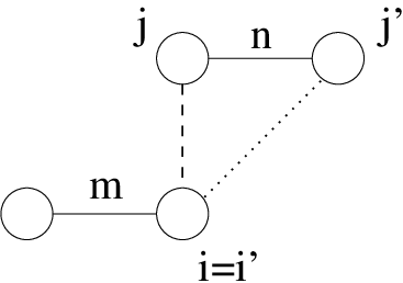
When the hopping term contains longer range hopping integrals such as $t^{\prime}$ and $t^{\prime\prime}$, it may happen that two bonds are connected by different hopping terms, as in Figure 2. We consider the factors of $\lambda$ in this case. Let us assume the nearest neighbor term has $\lambda_{i}\lambda_{j}$ whereas the longer-range term has $\lambda_{i^{\prime}}\lambda_{j^{\prime}}$ as in Figure 2. Now consider a symmetry operation of the lattice. If the operation exchanges the $1$-site and the $2$-site in bond $m$, both $\lambda_{i}$ and $\lambda_{i^{\prime}}$ change sign. Whereas if the operation exchanges the $1$-site and the $2$-site in bond $n$, both $\lambda_{j}$ and $\lambda_{j^{\prime}}$ change sign. It follows that the products $\lambda_{i}\lambda_{j}$ and $\lambda_{i^{\prime}}\lambda_{j^{\prime}}$ always change sign ‘in phase’ so that they are equal up to an overall sign. We define $\xi=\pm 1$ as the relative sign of the longer-range term with respect to the sign for nearest neighbor hopping (or exchange): $\lambda_{i^{\prime}}\lambda_{j^{\prime}}=\xi\lambda_{i}\lambda_{j}$. $\xi$ depends on the range of the hopping integral and for $t^{\prime}$ and $t^{\prime\prime}$ terms one finds $\xi=-1$. For any two sites $i$ and $j$ we define $\xi_{i,j}$ to be this relative sign for the hopping term which connects them.

The representation of the problem in terms of dimer states is exact but brings about no simplification so that approximations are necessary. As a first step, we re-interpret the singlet as the vacuum state of a dimer and accordingly replace the corresponding operators $s_{m}^{\dagger}$ and $s_{m}$ in (6) and (7) by unity. This is equivalent to the assumption that as in a Mott-insulator at half-filling the electrons in the lightly doped Mott insulator form an inert background - the ‘singlet soup’ - and that the only remaining active degrees of freedom are the spins of the electrons - represented by the triplets - and the doped holes, represented by the fermions. Replacing the singlet-operators in (6) and (7) by unity we obtain terms of 2^nd, 3^rd and 4^th order in triplet and fermion operators. The constraint (5) to have precisely one bond particle per dimer then becomes

$\displaystyle{\bf t}_{m}^{\dagger}\cdot{\bf t}_{m}+\sum_{\alpha\in\{\pm\}}\sum_{\sigma}f_{m,\alpha,\sigma}^{\dagger}f_{m,\alpha,\sigma}+e_{m}^{\dagger}e_{m}\in\{0,1\},$

(9)

which must hold for each bond $m$.

The constraint (9) is equivalent to an infinitely strong repulsive potential between bond particles in the same dimer. For small $x$, however, the density of triplets and fermions is small - this will be seen below and is crucial for the present theory. Namely for bose and fermi systems of low density it is known that even such infinitely strong repulsive interactions between particles do not qualitatively change the ground stateGalitskii; Beliaev. We therefore neglect the constraint assuming that it does not lead to a qualitative change of the results due to the low density of particles.
The problem with the infinitely strong repulsion between bond particles also occurs in the treatment of the Kondo lattice model. There it was found that good qualitative agreement with numerical results could be obtained by relaxing this constraint, and even quantitative agreement could be achieved by augmenting the energy of the bond particles by the loss of kinetic energy due to the blocking of bonds by a particlemykondo. However, to keep the present treatment simple we do not introduce this correction here. A more rigorous way to treat this repulsion has been carried out explicitely for bond bosons in spin systems by Kotov et al.Kotov and Shevchenko et al.Shevchenko.
Even with the approximation to reduce the number of active degrees of freedom we are far from a soluble problem, because the theory still refers to a given dimer covering of the lattice so that it is impossible to do any calculation for large systems. One might consider choosing a particular ‘simple’ dimer covering. However, since one is forced to make approximations, the exactness of the dimer representation is lost and the special symmetry of the covering will make itself felt in the approximate solutions resulting e.g. in an artificial supercell structure. On the other hand, the dimer Hamiltonian provides an exact representation of the original t-J model for any dimer covering of the plane. This means that for example the result for the spin correlation function $\langle{\bf S}_{j}(t)\cdot{\bf S}_{i}\rangle$ does not depend on the dimer covering in which the calculation is carried out. Put another way, the way in which a spin excitation propagates through the network of dimers from site $i\rightarrow j$ during the time $t$ does not depend at all on the geometry of the dimer covering. This might suggest to construct a translationally invariant approximate Hamiltonian by averaging the dimer Hamiltonian over all possible coverings. This means that now every bond in the lattice may be occupied by a bond particle, and the averaged Hamiltonian for two bonds $n$ and $m$ is $\bar{h}_{n,m}=\zeta\;h_{n,m}$ where $h_{n,m}$ is given by the sum of (6) and (7) and

$\displaystyle\zeta=\frac{N_{n,m}}{N_{d}}.$

(10)

Here $N_{n,m}$ is the number of dimer coverings which contain the bonds $n$ and $m$ and $N_{d}$ is the total number of dimer coverings. The resulting Hamiltonian obviously is translationally invariant and isotropic. To estimate $\zeta$ we use a crude approximation: consider two adjacent bonds as in Figure 3.

By symmetry the bond $m$ is covered by a dimer in exactly $1/4$ of all dimer coverings and we restrict ourselves to these. Assuming for simplicity that the number of coverings containing one of the three possible orientations of the adjacent bond $n$ are equal, we estimate $\zeta=\frac{1}{12}$. Later on, it will be seen that e.g. the spin gap depends sensitively on the value of $\zeta$ and we will consider it as an adjustable parameter but the values which give ‘reasonable’ results always are around $\zeta=0.1$.
In the averaged Hamiltonian there are additional unphysical configurations. For example, two bond particles may ‘cross’ each other, see Figure 4, and such configurations have to be excluded as well. This obviously amounts to an infinitely strong repulsion between the bond particles which acts whenever two bond particles share at least one site. Assuming the low-density limit we neglect this repulsion.
Lastly, we discuss the operator of electron number. If all dimers in a given covering are occupied by singlets or triplets, the number of electrons in the system is $N$. Each fermion reduces the number of electrons by one so if we discard the $e^{\dagger}$-boson

$\displaystyle x$

$\displaystyle=$

$\displaystyle\frac{1}{N}\;\sum_{m,\sigma}\;\left(\;f_{m,+,\sigma}^{\dagger}f_{m,+,\sigma}+f_{m,-,\sigma}^{\dagger}f_{m,-,\sigma}\;\right).$

(11)

Upon averaging we increase the number of bonds which can be occupied by a particle from $N/2$ to $2N$. However, we retain the expression (11) which guarantees a fermi surface with a volume propertional to the number of doped holes.
Lastly we mention the convention for the Fourier transform of bond operators. Defining $\rho_{m,\alpha}$ (with $\alpha\in\{x,y\}$) to be $1$ if $m$ is a bond in $\alpha$-direction and $0$ otherwise, the Fourier transform of a bond operator is (with $\alpha\in{x,y}$)

$$t_{{\bf k},\alpha}^{\dagger}=\frac{1}{\sqrt{N}}\;\sum_{m}\;\rho_{m,\alpha}\;e^{i{\bf k}{\bf R}_{m}}\;t_{m}^{\dagger}.$$

We next treat the bond particle Hamiltonian in Hartree-Fock approximation, thereby assuming a ground state which is invariant under spin rotationsSachdevBhatt; Gopalan. Accordingly, we drop the terms in (6) which are of 3^rd order in the triplets, and the terms in (7) which contain a single triplet or the vector poduct of two triplets. After Hartree-Fock decoupling these terms would give expectation values such as $\langle{\bf t}_{m}\rangle$ or $\langle{\bf t}_{m}^{\dagger}\times{\bf t}_{n}\rangle$ which vanish in a spin-rotation invariant state. For better clarity we give the remaining Hamiltonian after all approximations discussed so far have been made. The Hamiltonian is the sum of the following terms

	$\displaystyle H_{B}^{(0)}$	$\displaystyle=$	$\displaystyle J\;\sum_{m}{\bf t}_{m}^{\dagger}\cdot{\bf t}_{m}$
			$\displaystyle\;\;\;\;\;\;\;\;+\frac{\zeta}{4}\sum_{m<n}\;\sum_{i\in m\atop j\in n}J_{i,j}\lambda_{i}\lambda_{j}\;\left({\bf t}_{m}^{\dagger}\cdot{\bf t}_{n}+H.c.\right)$
			$\displaystyle\;\;\;\;\;\;\;\;\;\;\;\;\;\;+\frac{\zeta}{4}\sum_{m<n}\;\sum_{i\in m\atop j\in n}J_{i,j}\lambda_{i}\lambda_{j}\;\left({\bf t}_{m}^{\dagger}\cdot{\bf t}_{n}^{\dagger}+H.c.\right),$
	$\displaystyle H_{F}^{(0)}$	$\displaystyle=$	$\displaystyle-t\sum_{m,\sigma}\;\left(f_{m,+,\sigma}^{\dagger}f_{m,+,\sigma}-f_{m,-,\sigma}^{\dagger}f_{m,-,\sigma}\right)$
			$\displaystyle\;\;\;\;\;\;\;\;\;\;\;\;\;\;\;\;+\frac{\zeta}{4}\sum_{m,n}\;\sum_{i\in m\atop j\in n}t_{i,j}\;\sum_{\sigma}f_{n,j,\sigma}^{\dagger}f_{m,i,\sigma},$
	$\displaystyle H_{B}^{(1)}$	$\displaystyle=$	$\displaystyle-\frac{\zeta}{4}\sum_{m<n}\;\;\sum_{i\in m\atop j\in n}J_{i,j}\;({\bf t}_{n}^{\dagger}\times{\bf t}_{n})\cdot({\bf t}_{m}^{\dagger}\times{\bf t}_{m}),$
	$\displaystyle H_{B,F}^{(1)}$	$\displaystyle=$	$\displaystyle\frac{\zeta}{4}\sum_{m,n}\;\sum_{i\in m\atop j\in n}t_{i,j}\lambda_{i}\lambda_{j}\;{\bf t}_{m}^{\dagger}\cdot{\bf t}_{n}\;\sum_{\sigma}\;f_{n,j,\sigma}^{\dagger}f_{m,i,\sigma}.$

Here $J_{i,j}=J$ if $i$ and $j$ are nearest neighbors and zero otherwise. $H_{B}^{(0)}$ and $H_{F}^{(0)}$ are the noninteracting parts for bosons and fermions, $H_{B}^{(1)}$ describes the interaction between bosons, and $H_{B,F}^{(1)}$ the interaction between bosons and fermions. The double cross product in $H_{B}^{(1)}$ can be rewritten as

	$\displaystyle({\bf t}_{n}^{\dagger}\times{\bf t}_{n})\cdot({\bf t}_{m}^{\dagger}\times{\bf t}_{m})$	$\displaystyle=$	$\displaystyle\sum_{\lambda\neq\lambda^{\prime}}\;\left(t_{m,\lambda}^{\dagger}t_{n,\lambda}^{\dagger}\;t_{n,\lambda^{\prime}}t_{m,\lambda^{\prime}}-\right.$
			$\displaystyle\;\;\;\;\;\;\;\;\;\;\;\;\;\;\;\;\left.t_{m,\lambda}^{\dagger}t_{n,\lambda}\;t_{n,\lambda^{\prime}}^{\dagger}t_{m,\lambda^{\prime}}\right),$

where $\lambda,\lambda^{\prime}\in\{x,y,z\}$ denote the spin of the triplet. Upon mean-field factorization and using the spin-rotation invariance of the ground state this becomesGopalan

$\displaystyle\left(\frac{2}{3}\;\langle{\bf t}_{m}\cdot{\bf t}_{n}\rangle\;{\bf t}_{m}^{\dagger}\cdot{\bf t}_{n}^{\dagger}-\frac{2}{3}\;\langle{\bf t}_{m}^{\dagger}\cdot{\bf t}_{n}\rangle\;{\bf t}_{n}^{\dagger}\cdot{\bf t}_{m}\right)+H.c.$

The expectation values of products of two triplet operators thereby take the form

	$\displaystyle\langle{\bf t}_{m}^{\dagger}\cdot{\bf t}_{n}\rangle$	$\displaystyle=$	$\displaystyle\lambda_{i}\;\lambda_{j}\;\theta_{m,n},$
	$\displaystyle\langle{\bf t}_{m}\cdot{\bf t}_{n}\rangle$	$\displaystyle=$	$\displaystyle\lambda_{i}\;\lambda_{j}\;\eta_{m,n},$		(13)

where $i\in m$ and $j\in n$ are the sites where the exchange term acts and the ‘reduced expectation values’ $\theta_{m,n}$ and $\eta_{m,n}$ are identical for all symmetry equivalent pairs of bonds $m$, $n$. This follows from the fact that e.g. $(\lambda_{i}{\bf t}_{m})\;(\lambda_{j}{\bf t}_{n})$ is symmetry invariant by construction.
In the mean-field factorization of $H_{B,F}^{(1)}$ we again encounter the expectation values $\langle{\bf t}_{m}^{\dagger}\cdot{\bf t}_{n}\rangle$ and in addition fermionic expectation values. We define

$\displaystyle\chi_{m,n}$

$\displaystyle=$

$\displaystyle\sum_{i\in m\atop j\in n}\xi_{i,j}\frac{t_{i,j}}{t}\;\sum_{\sigma}\;\langle f_{m,i,\sigma}^{\dagger}f_{n,j,\sigma}\rangle.$

(14)

Thereby $\chi_{m,n}$ is the same for all symmetry equivalent pairs of bonds $m$, $n$ which follows from the fact that $f_{m,\nu,\sigma}^{\dagger}$ in (8) is symmetry-invariant by construction. The symmetry properties of $\theta_{m,n}$, $\eta_{m,n}$ and $\chi_{m,n}$ can also be verified by performing a Hartree-Fock calculation without imposing any symmetry properties of the expectation values - it turns out that the self-consistent expectation values always are the same for all symmetry-equivalent bonds.
Upon decoupling the boson-fermion interaction term $H_{B,F}^{(1)}$ we obtain two separate problems, one for the bosons, the other for the fermions. The bosonic mean-field Hamiltonian is

	$\displaystyle H_{B}$		$\displaystyle=J\sum_{m}\;{\bf t}_{m}^{\dagger}\cdot{\bf t}_{m}+$
			$\displaystyle\zeta\;\sum_{\langle m,n\rangle}\left[\;\left(\;\Delta_{m,n}\;{\bf t}_{m}^{\dagger}\cdot{\bf t}_{n}^{\dagger}+T_{m,n}\;{\bf t}_{m}^{\dagger}\cdot{\bf t}_{n}\;\right)+H.c.\;\right],$

where $\langle m,n\rangle$ indicates a sum over all pairs of bonds $m$ and $n$ connected by a nearest neighbor bond of the Hamiltonian and

	$\displaystyle\Delta_{m,n}$	$\displaystyle=$	$\displaystyle\lambda_{i}\lambda_{j}\;\;\;\frac{J}{4}\left(1-\frac{2}{3}\;\eta_{n,m}\right),$
	$\displaystyle T_{m,n}$	$\displaystyle=$	$\displaystyle\lambda_{i}\lambda_{j}\left[\,\frac{J}{4}\left(1+\frac{2}{3}\;\theta_{n,m}\right)+\frac{t}{4}\chi_{n,m,}\right].$		(16)

Thereby $i\in m$ and $j\in n$ are the sites where the exchange term acts - these are necessarily nearest neighbors.
The fermionic mean-field Hamiltonian is (omitting the spin index for brevity)

	$\displaystyle H_{F}$	$\displaystyle=$	$\displaystyle-t\;\sum_{m}\;\left(\;f_{m,+}^{\dagger}f_{m,+}-f_{m,-}^{\dagger}f_{m,-}\;\right)$
			$\displaystyle\;\;\;\;\;\;\;\;\;\;\;\;\;\;\;\;\;+\zeta\sum_{m,n}\;\sum_{i\in m\atop j\in n}\;\tilde{T}_{m,n}^{i,j}f_{m,i}^{\dagger}f_{n,j},$
	$\displaystyle\tilde{T}_{m,n}^{i,j}$	$\displaystyle=$	$\displaystyle\frac{t_{i,j}}{4}\;(1+\xi_{i,j}\theta_{n,m}).$		(17)

Thereby $\tilde{T}_{m,n}^{i,j}$ depends only on the type of hopping term ($t$, $t^{\prime}$ ot $t^{\prime\prime}$) which connects the sites $i$ and $j$ and is the same for all symmetry equivalent pairs of bonds $m$ and $n$. Inserting (8) we find

	$\displaystyle f_{m,i}^{\dagger}f_{n,j}$	$\displaystyle=$	$\displaystyle f_{m,+}^{\dagger}f_{n,+}-\lambda_{i}f_{m,-}^{\dagger}f_{n,+}$
			$\displaystyle\;\;\;\;\;\;\;\;-\lambda_{j}f_{m,+}^{\dagger}f_{n,-}+\lambda_{i}\lambda_{j}f_{m,-}^{\dagger}f_{n,-}.$

We consider $H_{B}$ in (). The parameters $\theta_{m,n}$, $\eta_{m,n}$ and $\chi_{m,n}$ are identical for all symmetry-equivalent pairs of bonds. In the following we replace e.g. $\theta_{m,n}\rightarrow\theta_{{\bf R}_{m}-{\bf R}_{n}}$ and the latter parameters are the same for all symmetry-equivalent distances. Fourier transformation of $H_{B}$ then gives

	$\displaystyle H$	$\displaystyle=$	$\displaystyle\frac{1}{2}\;\sum_{\bf k}\;\sum_{\alpha,\beta\in\{x,y\}}\;\left({\bf t}_{{\bf k},\alpha}^{\dagger}\Delta^{\alpha,\beta}_{\bf k}\;{\bf t}_{\beta,-{\bf k}}^{\dagger}+H.c.\right)$
			$\displaystyle\;\;\;\;\;\;\;\;\;\;\;\;\;\;\;\;\;\;\;\;+\sum_{\bf k}\;\;\sum_{\alpha,\beta\in\{x,y\}}{\bf t}_{{\bf k},\alpha}^{\dagger}\;\epsilon^{\alpha,\beta}_{\bf k}\;{\bf t}_{\beta,{\bf k}},$

with the $2\times 2$ matrices $\Delta_{\bf k}$ and $\epsilon_{\bf k}$ defined by

$\displaystyle\Delta^{\alpha,\beta}_{\bf k}$

$\displaystyle=$

$\displaystyle\frac{1}{N}\sum_{m,n}\;\rho_{m,\alpha}\;\Delta_{m,n}\;\rho_{n,\beta}\;e^{i{\bf k}\cdot({\bf R}_{n}-{\bf R}_{m})}$

and an analogous definition for $\epsilon^{\alpha,\beta}_{\bf k}$. We assume $\Delta_{m,n}$ and $T_{m,n}$ to be real so that $\epsilon_{-{\bf k}}=\epsilon^{*}_{\bf k}$ and $\Delta_{-{\bf k}}=\Delta^{*}_{\bf k}$. Both $\epsilon_{\bf k}$ and $\Delta_{\bf k}$ are Hermitean and $\epsilon_{\bf k}=J+\zeta\;\tilde{\epsilon}_{\bf k}$ with

	$\displaystyle\tilde{\epsilon}^{\;x,x}_{\bf k}$	$\displaystyle=$	$\displaystyle 4T_{(0,1)}\cos(k_{y})-2T_{(2,0)}\cos(2k_{x})$
			$\displaystyle\;\;\;\;\;\;\;\;\;\;\;\;\;\;\;\;\;\;\;\;\;-4T_{(1,1)}\cos(k_{x})\cos(k_{y}),$
	$\displaystyle\tilde{\epsilon}^{\;y,y}_{\bf k}$	$\displaystyle=$	$\displaystyle 4T_{(1,0)}\cos(k_{x})-2T_{(0,2)}\cos(2k_{y})$
			$\displaystyle\;\;\;\;\;\;\;\;\;\;\;\;\;\;\;\;\;\;\;\;\;-4T_{(1,1)}\cos(k_{x})\cos(k_{y}),$
	$\displaystyle\tilde{\epsilon}^{\;x,y}_{\bf k}$	$\displaystyle=$	$\displaystyle 4T_{(\frac{3}{2},\frac{1}{2})}\left(\;\sin(\frac{3k_{x}}{2})\sin(\frac{k_{y}}{2})\right.$
			$\displaystyle\;\;\;\;\;\;\;\;\;\;\;\;\;\;\;\;\;\;\;\;\;\left.+\sin(\frac{k_{x}}{2})\sin(\frac{3k_{y}}{2})\;\right).$

This can be verified using the signs of the products $\lambda_{i}\lambda_{j}$ in Figure 5. The expressions for $\Delta_{\bf k}$ are obtained from those for $\tilde{\epsilon}_{\bf k}$ by replacing $T_{{\bf R}}\rightarrow\Delta_{{\bf R}}$. To diagonalize $H$ we make the ansatz

	$\displaystyle{\bm{\tau}}_{\nu,{\bf k}}^{\dagger}\;\;\,$	$\displaystyle=$	$\displaystyle\sum_{\alpha\in\{x,y\}}\;\left(\;u_{\nu,{\bf k},\alpha}\;{\bf t}_{{\bf k},\alpha}^{\dagger}+v_{\nu,{\bf k},\alpha}\;{\bf t}_{-{\bf k},\alpha}\;\right),$
	$\displaystyle{\bm{\tau}}_{\nu,-{\bf k}}$	$\displaystyle=$	$\displaystyle\sum_{\alpha\in\{x,y\}}\;\left(\;v^{*}_{\nu,{\bf k},\alpha}\;{\bf t}_{{\bf k},\alpha}^{\dagger}+u^{*}_{\nu,{\bf k},\alpha}\;{\bf t}_{-{\bf k},\alpha}\;\right),$		(18)

where $\nu\in\{1,2\}$. Demanding $[\tau_{\nu,{\bf k}},\tau_{\mu,{\bf k}}^{\dagger}]=\delta_{\nu,\mu}$ leads to

$\displaystyle\sum_{\alpha\in\{x,y\}}\;\left(\;u^{*}_{\nu,{\bf k},\alpha}u_{\mu,{\bf k},\alpha}-v^{*}_{\nu,{\bf k},\alpha}v_{\mu,{\bf k},\alpha}\;\right)$

$\displaystyle=$

$\displaystyle\delta_{\nu,\mu}.$

(19)

whereas $[H,{\bm{\tau}}_{\nu,{\bf k}}^{\dagger}]=\omega_{\nu,{\bf k}}{\bm{\tau}}_{\nu,{\bf k}}^{\dagger}$ results in the non-Hermitean eigenvalue problem

$\displaystyle\left(\begin{array}[]{c c}\epsilon_{\bf k}&-\Delta_{\bf k}\\ \Delta^{*}_{-{\bf k}}&-\epsilon^{*}_{-{\bf k}}\end{array}\right)\;\left(\begin{array}[]{c}u_{\nu,{\bm{k}}}\\ v_{\nu,{\bm{k}}}\end{array}\right)$

$\displaystyle=$

$\displaystyle\omega_{\nu,{\bf k}}\;\left(\begin{array}[]{c}u_{\nu,{\bm{k}}}\\ v_{\nu,{\bm{k}}}\end{array}\right).$

For a matrix of the type on the left hand side it can be shown that the eigenvalues come in pairs of $\pm\omega$ and if $(u,v)$ is the right eigenvector for $+\omega$ then $(v^{*},u^{*})$ is the right eigenvector for $-\omega$ - which justifies the ansatz (18). Moreover $(u^{*},-v^{*})$ can be shown to be the left eigenvector for $+\omega$ so that (19) is equivalent to the condition that left and right eigenvectors for different eigenvalues are orthogonal - as it has to be. The mean-field Hamiltonian becomes

$\displaystyle H_{B}$

$\displaystyle=$

$\displaystyle\sum_{\bf k}\left(\sum_{\nu=1}^{2}\;\omega_{\nu,{\bf k}}\left({\bm{\bm{\tau}}}_{\nu,{\bf k}}^{\dagger}\;{\bm{\bm{\tau}}}_{\nu,{\bf k}}+\frac{3}{2}\right)-\frac{3}{2}\;tr(\epsilon_{\bf k})\right),$

and (18) can be reverted to give

	$\displaystyle{\bf t}_{{\bf k},\alpha}^{\dagger}\;\;\,$	$\displaystyle=$	$\displaystyle\sum_{\nu=1}^{2}\;\left(\;\;\;\,u_{\nu,{\bf k},\alpha}^{*}\;{\bm{\tau}}_{{\bf k},\nu}^{\dagger}-v_{\nu,{\bf k},\alpha}\;{\bm{\tau}}_{-{\bf k},\nu}\;\right),$
	$\displaystyle{\bf t}_{-{\bf k},\alpha}$	$\displaystyle=$	$\displaystyle\sum_{\nu=1}^{2}\;\left(\;-v_{\nu,{\bf k},\alpha}^{*}\;{\bm{\tau}}_{{\bf k},\nu}^{\dagger}+u_{\nu,{\bf k},\alpha}\;{\bm{\tau}}_{-{\bf k},\nu}\;\right).$

Using these expressions, the expectation values $\langle{\bf t}_{{\bf k},\alpha}^{\dagger}\cdot{\bf t}_{{\bf k},\beta}\rangle$ and $\langle{\bf t}_{{\bf k},\alpha}\cdot{\bf t}_{-{\bf k},\beta}\rangle$ can be obtained, from which the parameters $\theta_{m,n}$ and $\eta_{m,n}$ in (13) can be calculated.

We consider the fermionic Hamiltonian (17). Fourier transformation gives $H_{F}=\sum_{\bf k}H_{F,{\bf k}}$

	$\displaystyle H_{F,{\bf k}}$	$\displaystyle=$	$\displaystyle-t\sum_{\alpha\in\{x,y\}}\left(f_{{\bf k},\alpha,+}^{\dagger}f_{{\bf k},\alpha,+}-f_{{\bf k},\alpha,-}^{\dagger}f_{{\bf k},\alpha,-}\right)$		(27)
			$\displaystyle\;\;\;\;\;\;\;\;\;\;\;\;\;\;\;\;\;\;\;\;\;\;\;\;\;\;\;\;\;\;\;\;\;\;\;+\zeta\;v_{\bf k}^{\dagger}\tilde{H}_{\bf k}v_{\bf k}$

where the vector $v_{\bf k}=(f_{k,x,+},f_{k,y,+},f_{k,x,-},f_{k,y,-})^{T}$ has been introduced. Here we give the elements of the $4\times 4$ matrix $\tilde{H}_{\bf k}$ for the case that the t-J Hamiltonian contains only nearest neighbor hopping:

	$\displaystyle\tilde{H}_{1,1}$	$\displaystyle=$	$\displaystyle 4\tilde{T}_{(0,1)}\cos(k_{y})+4\tilde{T}_{(1,1)}\cos(k_{x})\cos(k_{y})+2\tilde{T}_{(2,0)}\cos(2k_{x})$
	$\displaystyle\tilde{H}_{1,2}$	$\displaystyle=$	$\displaystyle 4\left(\;\tilde{T}_{(\frac{3}{2},\frac{1}{2})}\cos(\frac{3k_{x}}{2})\cos(\frac{k_{y}}{2})+\tilde{T}_{(\frac{1}{2},\frac{3}{2})}\cos(\frac{k_{x}}{2})\cos(\frac{3k_{y}}{2})\;\right)$
	$\displaystyle\tilde{H}_{1,3}$	$\displaystyle=$	$\displaystyle-2i\left(\;2\tilde{T}_{(1,1)}\sin(k_{x})\cos(k_{y})+\tilde{T}_{(2,0)}\sin(2k_{x})\;\right)$
	$\displaystyle\tilde{H}_{1,4}$	$\displaystyle=$	$\displaystyle-4i\left(\;\;\tilde{T}_{(\frac{3}{2},\frac{1}{2})}\cos(\frac{3k_{x}}{2})\sin(\frac{k_{y}}{2})+\tilde{T}_{(\frac{1}{2},\frac{3}{2})}\cos(\frac{k_{x}}{2})\sin(\frac{3k_{y}}{2})\;\right)$
	$\displaystyle\tilde{H}_{2,2}$	$\displaystyle=$	$\displaystyle 4\tilde{T}_{(1,0)}\cos(k_{x})+4\tilde{T}_{(1,1)}\cos(k_{x})\cos(k_{y})+2\tilde{T}_{(0,2)}\cos(2k_{y})$
	$\displaystyle\tilde{H}_{2,3}$	$\displaystyle=$	$\displaystyle-4i\left(\;\tilde{T}_{(\frac{3}{2},\frac{1}{2})}\sin(\frac{3k_{x}}{2})\cos(\frac{k_{y}}{2})+\tilde{T}_{(\frac{1}{2},\frac{3}{2})}\sin(\frac{k_{x}}{2})\cos(\frac{3k_{y}}{2})\;\right)$
	$\displaystyle\tilde{H}_{2,4}$	$\displaystyle=$	$\displaystyle-2i\left(\;2\tilde{T}_{(1,1)}\cos(k_{x})\sin(k_{y})+\tilde{T}_{(0,2)}\sin(2k_{y})\;\right)$
	$\displaystyle\tilde{H}_{3,3}$	$\displaystyle=$	$\displaystyle 4\tilde{T}_{(0,1)}\cos(k_{y})-4\tilde{T}_{(1,1)}\cos(k_{x})\cos(k_{y})-2\tilde{T}_{(2,0)}\cos(2k_{x})$

	$\displaystyle\tilde{H}_{3,4}$	$\displaystyle=$	$\displaystyle 4\left(\;\tilde{T}_{(\frac{3}{2},\frac{1}{2})}\sin(\frac{3k_{x}}{2})\sin(\frac{k_{y}}{2})+\tilde{T}_{(\frac{1}{2},\frac{3}{2})}\sin(\frac{k_{x}}{2})\sin(\frac{3k_{y}}{2})\;\right)$
	$\displaystyle\tilde{H}_{4,4}$	$\displaystyle=$	$\displaystyle 4\tilde{T}_{(1,0)}\cos(k_{x})-4\tilde{T}_{(1,1)}\cos(k_{x})\cos(k_{y})-2\tilde{T}_{(0,2)}\cos(2k_{y})$

Note that on the respective right-hand side we have used the notation $\tilde{T}_{m,n}\rightarrow\tilde{T}_{{\bf R}_{m}-\bf{R}_{n}}$ and dropped the superscripts on $\tilde{T}$ because they all refer to nearest neighbors. The terms in $\tilde{H}$ originating from longer range hopping integrals such as $t^{\prime}$ and $t^{\prime\prime}$ are also easily written down but the resulting expressions are lengthy so we do not give them here.
Diagonalizing $-(H_{F,{\bf k}}-\mu)$ we obtain the dispersion $E_{\nu,{\bf k}}$ (with $\nu=1\dots 4$) for the electron-like quasiparticles and the corresponding eigenvectors ${\bf e}_{\nu,{\bf k}}$, from which the mean-field expectation values $\chi_{n,m}$ (14) can be calculated. This allows to perform the self-consistency procedure, thereby using Broyden’s algorithmBroyden for better convergence, and obtain the self-consistent values of the bosonic parameters $\theta_{m,n}$ and $\eta_{m,n}$ in (13) and $\chi_{n,m}$ (14).

References

- (1) B. Keimer, S. A. Kivelson, M. R. Norman, S. Uchida, J. Zaanen Nature 518, 179 (2015).
- (2) A. G. Loeser, Z.-X. Shen, D. S. Dessau, D. S. Marshall, C. H. Park, P. Fournier, and A. Kapitulnik, Science 273, 325 (1996).
- (3) H. Ding, T. Yokoya, J. C. Campuzano, T. Takahashi, M. Randeria, M. R. Norman, T. Mochiku, K. Kadowaki, and J. Giapintzakis, Nature 382, 51 (1996).
- (4) A. Damascelli, Z. Hussain, and Z.-X. Shen, Rev. Mod. Phys. 75, 473 (2003).
- (5) B. O. Wells, Z.-X. Shen, A. Matsuura, D. M. King, M. A. Kastner, M. Greven, and R. J. Birgeneau, Phys. Rev. Lett. 74, 964 (1995).
- (6) F. Ronning, C. Kim, D. L. Feng, D. S. Marshall, A. G. Loeser, L. L. Miller, J. N. Eckstein, L. Bozovic, and Z.-X. Shen, Science 282, 2067 (1998).
- (7) T. Kondo, A. D. Palczewski, Y. Hamaya, T. Takeuchi, J. S. Wen, Z. J. Xu, G. Gu, and A. Kaminski, Phys. Rev. Lett. 111, 157003 (2013).
- (8) H.-B. Yang, J. D. Rameau, Z.-H. Pan, G. D. Gu, P. D. Johnson, H. Claus, D. G. Hinks, and T. E. Kidd, Phys. Rev. Lett. 107, 047003 (2011).
- (9) K. Tanaka, W. S. Lee, D. H. Lu, A. Fujimori, T. Fujii, Risdiana, I. Terasaki, D. J. Scalapino, T. P. Devereaux, Z. Hussain, Z.-X. Shen, Science 314, 1910 (2006).
- (10) M. Hashimoto, R.-H. He, K. Tanaka, J.-P. Testaud, W. Meevasana, R. G. Moore, D. Lu, H. Yao, Y. Yoshida, H. Eisaki, T. P. Devereaux, Z. Hussain, and Z.-X. Shen, Nature Phys. 6, 414 (2010).
- (11) H. Eskes and R. Eder, Phys. Rev. B. 54, R14226 (1996).
- (12) R. Eder und K. W. Becker, Phys. Rev. B 44, 6982 (1991).
- (13) O. P. Sushkov, G. A. Sawatzky, R. Eder and H. Eskes, Phys. Rev. B. 56, 11769 (1997).
- (14) J. M. Tranquada, B. J. Sternlieb, J. D. Axe, Y. Nakamura,S. Uchida, Nature 375, 561 (1995).
- (15) C. Howald, H. Eisaki, N. Kaneko, M. Greven, and A. Kapitulnik, Phys. Rev. B 67, 014533 (2003).
- (16) G. Ghiringhelli, M. Le Tacon, M. Minola, S. Blanco-Canosa, C. Mazzoli, N. B. Brookes, G. M. De Luca, A. Frano, D. G. Hawthorn, F. He, T. Loew, M. Moretti Sala, D. C. Peets, M. Salluzzo, E. Schierle, R. Sutarto, G. A. Sawatzky, E. Weschke, B. Keimer2, and L. Braicovich, Science 337, 821 (2012).
- (17) S. I. Mirzaei, D. Stricker, J. N. Hancock, C. Berthod, A. Georges, E. van Heumen, M. K. Chan, X. Zhao, Y. Li, M. Greven, N. Barisic, and D. van der Marel, Proc. Natl. Acad. Sci. U.S.A. 110, 5774 (2013).
- (18) Y. Ando, Y. Kurita, S. Komiya, S. Ono, and K. Segawa, Phys. Rev. Lett. 92, 197001 (2004).
- (19) N. Barisic, M. K. Chan, Y. Li, G. Yu, X. Zhao, M. Dressel, A. Smontara, and M. Greven, Proc. Natl. Acad. Sci. U.S.A. 110, 12235 (2013).
- (20) G. Grissonnanche, F. Laliberte, S. Dufour-Beausejour, M. Matusiak, S. Badoux, F. F. Tafti, B. Michon, A. Riopel, O. Cyr-Choiniere, J. C. Baglo, B. J. Ramshaw, R. Liang, D. A. Bonn, W. N. Hardy, S. Kramer, D. LeBoeuf, D. Graf, N. Doiron-Leyraud, and L. Taillefer, Phys. Rev. B 93, 064513 (2016).
- (21) M. K. Chan, M. J. Veit, C. J. Dorow, Y. Ge, Y. Li, W. Tabis, Y. Tang, X. Zhao, N. Barisic, and M. Greven, Phys. Rev. Lett. 113, 177005 (2014).
- (22) J. W. Loram, K. A. Mirza, J. M. Wade, J. R. Cooper, N. Athanassopoulou, and W. Y. Liang, Advances in Superconductivity VII, K. Yamafuji and T. Morishita, (Eds.) Springer (1995).
- (23) S. Badoux, W. Tabis, F. Laliberte, G. Grissonnanche, B. Vignolle, D. Vignolles, J. Beard, D. A. Bonn, W. N. Hardy, R. Liang, N. Doiron-Leyraud, L. Taillefer, and C. Proust, Nature 531, 210 (2016) .
- (24) C. Collignon, S. Badoux, S. A. A. Afshar, B. Michon, F. Laliberte, O. Cyr-Choiniere, J.-S. Zhou, S. Licciardello, S. Wiedmann, N. Doiron-Leyraud, and L. Taillefer, Phys. Rev. B 95, 224517 (2017).
- (25) N. P. Ong, Z. Z. Wang, J. Clayhold, J. M. Tarascon, L. H. Greene, and W. R. McKinnon Phys. Rev. B 35, 8807 (1987).
- (26) H. Takagi, T. Ido, S. Ishibashi, M. Uota, S. Uchida, and Y. Tokura, Phys. Rev. B 40, 2254 (1989).
- (27) W. J. Padilla, Y. S. Lee, M. Dumm, G. Blumberg, S. Ono, K. Segawa, S. Komiya, Y. Ando, and D. N. Basov Phys. Rev. B 72, 060511(R) (2005).
- (28) J. Tallon and J. Loram, Physica C 349, 53 (2001).
- (29) N. Doiron-Leyraud, C. Proust, D. LeBoeuf, J. Levallois, J.-B. Bonnemaison, R. Liang, D. A. Bonn, W. N. Hardy, and L. Taillefer, Nature 447, 565 (2007).
- (30) S. E. Sebastian, N. Harrison, M. M. Altarawneh, C. H. Mielke, R. Liang, D. A. Bonn, and G. G. Lonzarich, Proc. Natl. Acad. Sci. U.S.A. 107, 6175 (2010).
- (31) M. K. Chan, N. Harrison, R. D. McDonald, B. J. Ramshaw, K. A. Modic, N. Barisic, and M. Greven, Nature Communications 7, 12244 (2016).
- (32) C. Proust, B. Vignolle, J. Levallois, S. Adachi, N. E. Hussey, Proc. Natl. Acad. Sci. U.S.A. 113, 13654 (2016).
- (33) D. LeBoeuf, N. Doiron-Leyraud, J. Levallois, R. Daou, J.-B. Bonnemaison, N. E. Hussey, L. Balicas, B. J. Ramshaw, R. Liang, D. A. Bonn, W. N. Hardy, S. Adachi, C. Proust, and L. Taillefer, Nature 450, 533 (2007).
- (34) B.J. Ramshaw, B. Vignolle, J. Day, R. Liang, W. Hardy, C. Proust, and D.A. Bonn, Nature Phys. 7 234 (2011).
- (35) R. Comin, A. Frano, M. M. Yee, Y. Yoshida, H. Eisaki, E. Schierle, E. Weschke, R. Sutarto, F. He, A. Soumyanarayanan, Yang He, M. Le Tacon, I. S. Elfimov, J. E. Hoffman, G. A. Sawatzky, B. Keimer, and A. Damascelli, Science, 343, 390 (2014).
- (36) R. Eder and Y. Ohta, Phys. Rev. B 51, 6041 (1995).
- (37) S. Nishimoto, Y. Ohta, and R. Eder, Phs. Rev. B 57, R5590 (1998).
- (38) D. L. Feng, N. P. Armitage, D. H. Lu, A. Damascelli, J. P. Hu, P. Bogdanov, A. Lanzara, F. Ronning, K. M. Shen, H. Eisaki, C. Kim, J.-i. Shimoyama, K. Kishio, and Z.-X. Shen, Phys. Rev. Lett. 86, 5550 (2001).
- (39) Y.-D. Chuang, A. D. Gromko, A. Fedorov, Y. Aiura, K. Oka, Yoichi Ando, H. Eisaki, S. I. Uchida, and D. S. Dessau, Phys. Rev. Lett. 87, 117002 (2001).
- (40) M. Plate, J. D. F. Mottershead, I. S. Elfimov, D. C. Peets, Ruixing Liang, D. A. Bonn, W. N. Hardy, S. Chiuzbaian, M. Falub, M. Shi, L. Patthey, and A. Damascelli Phys. Rev. Lett. 95, 077001 (2005).
- (41) N. E. Hussey, M. Abdel-Jawad, A. Carrington, A. P. Mackenzie, and L. Balicas,
- (42) B. Vignolle, A. Carrington, R. A. Cooper, M. M. J. French, A. P. Mackenzie, C. Jaudet, D. Vignolles, C. Proust and N. E. Hussey, Nature 455, 952 (2008).
- (43) S. Nakamae, K. Behnia, N. Mangkorntong, M. Nohara, H. Takagi, S. J. C. Yates, and N. E. Hussey, Phys. Rev. B 68, 100502(R) (2003).
- (44) R. Eder and Y. Ohta, Phys. Rev. B 51, 11683 (1995).
- (45) R. Eder, Y. Ohta, and S. Maekawa, Phys. Rev. Lett. 74, 5124 (1995).
- (46) S. Sachdev and R. N. Bhatt, Phys. Rev. B 41, 9323 (1990).
- (47) S. Chakravarty, C. Nayak, and S. Tewari, Phys. Rev. B 68, 100504(R) (2003).
- (48) S. Chakravarty and H.-Y. Kee, Proc. Natl. Acad. Sci. USA 105, 8835 (2008).
- (49) Y. Qi and S. Sachdev Phys. Rev. B 81, 115129 (2010).
- (50) Eun Gook Moon and Subir Sachdev Phys. Rev. B 83, 224508 (2011).
- (51) M. Punk and S. Sachdev, Phys. Rev. B 85, 195123 (2012).
- (52) M. Holt, J. Oitmaa, W. Chen, and O. P. Sushkov, Phys. Rev. Lett. 109, 037001 (2012).
- (53) M. Holt, J. Oitmaa, W. Chen, and O. P. Sushkov Phys. Rev. B 87, 075109 (2013).
- (54) D. Senechal and A.-M. S. Tremblay, Phys. Rev. Lett. 92, 126401 (2004).
- (55) B. Kyung, S. S. Kancharla, D. Senechal, A.-M. S. Tremblay, M. Civelli, and G. Kotliar, Phys. Rev. B 73, 165114 (2006).
- (56) T. M. Rice, K.-Y. Yang, and F. C. Zhang, Rep. Prog. Phys. 75 016502 (2012).
- (57) J.-X. Li, C.-Q. Wu, and D.-H. Lee, Phys. Rev. B 74, 184515 (2006)
- (58) J. Hubbard, Proc. Roy. Soc. London, Ser. A 277, 237 (1964).
- (59) R. Eder, P. Wrobel, and Y. Ohta, Phys. Rev. B 82, 155109 (2010).
- (60) M. Punk, A. Allais, and S. Sachdev, Proc. Natl. Acad. Sci. U.S.A. 112, 9552 (2015).
- (61) S. Huber, J. Feldmeier, and M. Punk, Phys. Rev. B 97, 075144 (2018).
- (62) J. Feldmeier, S. Huber, and M. Punk, Phys. Rev. Lett. 120, 187001 (2018).
- (63) S. Gopalan, T. M. Rice, and M. Sigrist, Phys. Rev. B 49, 8901 (1994).
- (64) O. P. Sushkov, Phys. Rev. B 60, 3289 (1999).
- (65) C. Jurecka and W. Brenig, Phys. Rev. B 63, 094409 (2001).
- (66) M. Vojta and K. W. Becker, Phys. Rev. B 60, 15201 (1999).
- (67) S. Ray and M. Vojta, Phys. Rev. B 98, 115102 (2018).
- (68) O. P. Sushkov, Phys. Rev. B 63, 174429 (2001).
- (69) K. Park and S. Sachdev, Phys. Rev. B 64, 184510 (2001).
- (70) M. Siahatgar, B. Schmidt, G. Zwicknagl, and P. Thalmeier, New J. Phys. 14, 103005 (2014).
- (71) K. A. Chao, J. Spalek, A. M. Oles, J. Phys. C10, L 271 (1977).
- (72) F. C. Zhang, T. M. Rice, Phys. Rev. B 37, 3759 (1988).
- (73) V. M. Galitskii, Sov. Phys. JETP. 7, 104 (1958).
- (74) S. T. Beliaev, Sov. Phys. JETP. 7, 299 (1958).
- (75) V. N. Kotov, O. Sushkov, ZhengWeihong, and J. Oitmaa, Phys. Rev. Lett. 80, 5790 (1998).
- (76) P. V. Shevchenko, A. W. Sandvik, and O. P. Sushkov Phys. Rev. B 61, 3475 (2000).
- (77) D. D. Johnson, Phys. Rev. B. 38, 12807, (1988).
- (78) M. Fujita, H. Hiraka, M. Matsuda, M. Matsuura, J. M. Tranquada, S. Wakimoto, G. Xu, and K. Yamada, J. Phys. Soc. Jpn. 81, 011007 (2012).
- (79) M. K. Chan, C. J. Dorow, L. Mangin-Thro, Y. Tang, Y. Ge, M. J. Veit, G. Yu, X. Zhao, A. D. Christianson, J. T. Park, Y. Sidis, P. Steffens, D. L. Abernathy, P. Bourges, and M. Greven, Nature Communications 7, 10819 (2016).
- (80) M. Le Tacon, G. Ghiringhelli, J. Chaloupka, M. Moretti Sala, V. Hinkov, M. W. Haverkort, M. Minola, M. Bakr, K. J. Zhou, S. Blanco-Canosa, C. Monney, Y. T. Song, G. L. Sun, C. T. Lin, G. M. De Luca, M. Salluzzo, G. Khaliullin, T. Schmitt, L. Braicovich, and B. Keimer, Nature Physics 7, 725 (2011).
- (81) L. N. Bulaevskii, E. L. Nagaev, and D. L. Khomskii, Sov. Phys. JETP. 27, 836 (1968).
- (82) S. A. Trugman, Phys. Rev. 37, 1597 (1988); ibid Phys. Rev. B 41, 892 (1990).
- (83) R. Eder and K. W. Becker, Z. Phys. B 78, 219 (1990).
- (84) G. Martinez and P. Horsch, Phys. Rev. B 44, 317 (1991).
- (85) W. Chen and O. P. Sushkov Phys. Rev. B 88, 184501 (2013).
- (86) R. Eder, K. Grube, and P. Wróbel, Phys. Rev. B 93, 165111 (2016).
- (87) R. Eder and P. Wróbel, Phys. Rev. B 98, 245125 (2018).
- (88) R. Eder, Phys. Rev. B 99, 085134 (2019).
- (89) P. A. Lee, N. Nagaosa, and X.-G. Wen, Rev. Mod. Phys. 78, 17 (2006).