Scattering of light with angular momentum from an array of particles
Abstract
Understanding the scattering properties of various media is of critical importance in many applications, from secure, high-bandwidth communications to extracting information about biological and mineral particles dissolved in sea water. In this paper we demonstrate how beams carrying orbital angular momentum (OAM) can be used to detect the presence of symmetric or chiral subsets of particles in disordered media. Using a generalized Mie theory we calculate analytical expressions for quasi-monochromatic structured light scattered by dilute distributions of micro- and nanoparticles. These allow us to determine the angular momentum of the scattered field as a function of the angular momentum of the incident beam and of the spatial distributions of scattering particles. Our numerical results show that we can distinguish structured from random distributions of particles, even when the number density of ordered particles is a few percent of the total distribution. We also find that the signal-to-noise ratio, in the forward direction, is equivalent for all orders of the Laguerre-Gaussian modes in relatively dense (but still dilute) distributions, making them an ideal basis to encode and transmit multiplexed signals.
I Introduction
Light carrying orbital angular momentum (OAM) has attracted a great deal of interest due to its potential to enhance many applications, including high-resolution imaging Klar et al. 2000, and optical trapping and manipulation of micro- and nanoparticlesHe et al. 1995. It is also of significant interest as a resource in high capacity quantum communication and information systems. Unlike the spin angular momentum (SAM) associated with circular polarization, OAM is not restricted to two orthogonal states. Large amounts of information can then be carried by single photons, opening the door to new protocols for quantum key distribution with significantly increased data transfer rates Tyler and Boyd 2009.
As any communications system relies on the fidelity of the signal after propagation, it is essential to understand the effect of the medium that they travel through. In this case we focus on the effect of propagation through scattering media. Whether this be due to scattering by aerosols in the atmosphere or by phytoplankton or mineral particles in natural waters Mobley 1994, scattering will contribute both to the coherence and attenuation of the signal, resulting in a loss of information and a reduction in the fidelity of the system.
While scattering is considered to be detrimental for applications in information transfer, the ability to measure the power of the OAM states of the scattered light Leach et al. 2004; Berkhout et al. 2010; Dudley et al. 2013; Mirhosseini et al. 2013; Gu et al. 2018; Fontaine et al. 2019 may provide a source of information about the properties of the scattering medium, from the size and type of the particulates to their geometrical distribution, that has not yet been exploited. This may be of particular benefit for environmental sensing and metrology, and ocean transmissometry, and may even find applications in biological imaging. Another area of potential application is nanophotonics, where some of the unique features of the scattering of light carrying OAM can reveal the fraction of ordered and disordered nanoparticles within complex nanostructures.
In this paper we present a theory for quasi-monochromatic structured light scattered by dilute distributions of micro- and nanoparticles that allows us to determine the angular momentum components of the scattered field in the far field zone as a function of the total angular momentum of the incident beam along its axis and of the dielectric properties and spatial distributions of the scattering particles. For paraxial incident fields, we show that it is possible to detect the presence of subsets of symmetric and chiral particles simply by controlling the OAM of the incident beams and measuring the resultant OAM of the scattered fields in the far field. This may help us to detect objects hidden in scattering media Cochenour et al. 2017 or to visualize flows resulting in geometrically ordered concentrations of particles Balkovsky et al. 2001. Here we consider both the case of particles distributed over volumes with dimensions several orders of magnitude larger than the wavelength of light, and the case of particles distributed over volumes with dimensions of a few tens of the wavelength. The first case is typical of marine optics Mobley 1994 and atmospheric science, or of nanophotonic experiments with nanoparticles in solutions. The second case is typical of experiments involving particles held in optical traps or forming artificial nanophotonics structures Grier 2003; Polin et al. 2006; Di Leonardo et al. 2007; Curran et al. 2010. We show that controlling the OAM of the incident beam and measuring the power of the light scattered in different OAM states allows us to identify the presence of subsets of particles forming polygonal or chiral structures in both cases. We also demonstrate that OAM can be used to improve the signal to noise ratio, a result that can be useful in reducing the error due to scattering both in measures of absorption, and in communications applications.
As the theory is necessarily very mathematical, we start by giving an outline of our method and our main theoretical results. We then present a number of numerical results highlighting the main features and capabilities of our theory. For the sake of simplicity and to facilitate the comparisons between theory and experiments, our numerical results have been obtained using distributions of gold nanospheres as these are used in many experiments. However, we stress that our theory is applicable to any type of scattering particles and host medium, provided that multiple scattering can be neglected. For the interested reader, we then present a detailed outline of our theory.
II Overview of Theory and Main Results
We consider an experimental set-up, as shown in Fig. 1, where light beams propagating along the -axis are incident on distributions of micro- and nanoparticles with dielectric permitivitty and magnetic permeability immersed in a uniform isotropic dielectric medium with different electromagnetic properties. Using a generalized Mie theory, we calculate the far field scattering of both random and symmetric distributions of particles in which multiple scattering can be neglected and we can safely consider the total scattered field as the coherent sum of the fields scattered by the individual particles. Our theory is applicable to any type of scattering particle and host medium and is developed for arbitrary particles and beams.
From a physical point of view, the key issue is that we expand the field scattered by particles in different positions in electric and magnetic multipolar waves Biedenharn and Louck 1985, and , where, for each particle, is the total angular momentum with respect to the center of the particle and is its component parallel to the direction of propagation of the incident beam in non-dimensional units. However , the total angular momentum of the scattered waves and along the axis of the incident beam, is not and depends on the distance between the centers of the off-axis scattering particles and the axis of the incident beam. The essential features of scattering from dilute distributions of particles depend on this property and on the fact that waves scattered by different particles are coherent. Due to the coherent addition of the scattered waves, structured incident beams can be used to induce collective scattering that reveals the spatial structure of the particles’ distributions. More specifically, one can detect the presence of subsets of particles arranged with the roto-reflection symmetry of regular polygons with sides, or chiral structures. It is also possible to detect the position of the symmetry axes of two and three dimensional arrays and chiral structures by displacing the particles with respect to the incident beam’s axis and measuring the spread of the scattered light power over the component of OAM along the beam axis of the scattered field, . The resolution on the transverse position of symmetry axes, or the centers of chiral structures, is of a few percent of the transverse dimension of the incident beam.
For the incident beams considered here, the main theoretical results depend on the angular momentum of the incident beam and the types and distributions of the particles. The main results can be summarized as follows:
- •
The multipolar waves and , scattered by every particle, combine in a scattered wave with total angular momentum along the axis of the beam . In non-dimensional units, is the total angular momentum along the beam’s axis ; is the component of OAM of the incident Laguerre-Gauss beam along its axis; defines the spatial harmonics of the multipole-multipole distributions, , where is the azimuthal angle.
- •
For light, the component of the spin along the propagation axis takes three values: for polarization , and for polarization . The component of OAM along the beam axis of the scattered field, , can also take three values for any given , as .
- •
In the forward and backward directions, only the terms with both and do not vanish.
- •
In the forward direction most particles scatter in phase. The positions of the particles only affect the scattering amplitude in the forward direction through the slowly varying amplitude of the incident field.
- •
In the backward direction the scattered fields of most particles will cancel out. This is due to rapidly varying phase terms that depend on the coordinates of the particles along the direction of propagation of the incident beam. The exceptions to this are particles that either all lie on a plane orthogonal to the propagation axis or are periodically distributed along the direction of propagation of the incident beam, as the fields scattered by these particles add in phase in the backward direction.
III Numerical results
In this section we show how incident beams carrying OAM can be used to extract information about the spatial structure of distributions of scattering particles. A schematic showing the essential components of the type of experimental setup we envisage is shown in Fig. 1: with respect to the theory developed here, the key features are provided by the OAM sorters that determine the OAM of the incident beam and enable measurements of the distribution of the scattered field power over different OAM values Leach et al. 2004; Berkhout et al. 2010; Dudley et al. 2013; Mirhosseini et al. 2013; Gu et al. 2018; Fontaine et al. 2019.

This problem has several very different spatial scales that need to be considered carefully: the wavelength of the incident and scattered fields, the largest dimension of the particles, , the transverse and longitudinal dimensions of the distribution, and , as well as the transverse dimension of the incident beam, , and its coherence length . We consider only arrays of particles with inter-particle distances such that multiple scattering can be neglected Berg et al. 2008 and with , where the total scattered field is the coherent sum of all the fields scattered by each particle. We note that the latter condition is not a limit to this theory. For the case the distribution can be divided into sections of length with the total field being the incoherent sum of the resulting fields from each section.
Our numerical results are obtained by considering paraxial Laguerre-Gaussian beams and spheres with radii , where is the beam waist and is the corresponding Rayleigh parameter, . As we show later in the theory section, only corrections to the paraxial fields of order affect the scattered fields; for the cases considered here, corrections of this order can be safely neglected. For simplicity, we consider only the “purely azimuthal” modes (), although the radial modes could provide additional information, as discussed in Sec. IV.
As mentioned above, our theory is applicable to any type of scattering particles and host medium. However, again for the sake of simplicity, and to facilitate the comparisons between theory and experiments, our numerical results have been obtained using distributions of gold nanospheres with radii of nm. We use the Lorentz-Drude dielectric function Rakić et al. 1998 to model the electromagnetic response of the particles. As a result of their size and dielectric function these particles have a spectrally resolved Mie-type resonance with a peak around nm for the scattered fields. Using a different dielectric function would affect the position of the resonance Imura et al. 2014, but would not affect the ability to identify spatial properties of the particles’ distributions which depends on the general properties of the scattering process.
III.1 Ordered and disordered particle distributions
We first consider particles distributed over volumes with dimensions much larger than the wavelength, as is the case in nanophotonics with large numbers of nanoparticles in colloids or in marine optics. In particular, we investigate:
- 1.
Nanoparticles randomly distributed within a cylindrical volume, with radius of cross-section ;
- 2.
Particles regularly distributed, on layers orthogonal to the -axis, along lines with the symmetry of regular -sided polygons;
- 3.
Combinations of the previous two types of distributions.
Information on the distribution of particles is most easily extracted from either backward or forward scattering, so we consider these simple cases first. We use the index to label the spheres and the azimuthal moments of the particles’ distribution, defined as , to identify random, partially ordered and ordered distributions. The azimuthal moments are especially useful when considering two dimensional structures and for forward scattering, where the scattered fields depends very weakly on the position of the particles along the (beam) axis. For identical particles, the azimuthal moments are proportional to the volume integral of the azimuthal Fourier components of the particles’ distributions, as we show in Sec. IV.
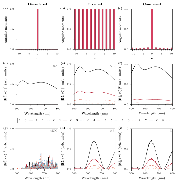
Along the top row of Fig. 2 we plot the azimuthal moments of the distribution of particles: for the random distribution the order moment is dominant, while for the ordered distribution with -fold symmetry, the even order moments are all of equal amplitude. The presence of the -fold symmetry is clearly evident even when the number of ordered particles is only of the total distribution. In the second and third rows of Fig. 2 we plot the forward and backward scattering, respectively, for incident beams with OAM () ranging from to for each of these distributions. Our results illustrate that only the terms with and either , or do not vanish. Note that the forward scattering intensity shown is proportional to the modulus squared of the sum of the scattering amplitudes of the electric and magnetic multipoles in the forward direction due to the spatial harmonics of the distribution. For forward scattering, the scattered fields only depend on the positions of the particles over the long length scales and of the paraxial incident beam, so many particles add up in phase. For backward scattering, however, the scattered fields depend on the -coordinates of the particles along the beam’s axis over the short length scale . The relative phases depend on the wavelength of the incident field and for most wavelengths the backward scattered fields of random distributions are not in phase. There are, however, some wavelengths for which partial coherence gives rise to larger values of the backward scattered field. Fields scattered by particles lying on a plane orthogonal to the beam axis are in phase, hence we observe interference fringes for symmetric distributions over two or more planes orthogonal to the beam axis. As the fields scattered by a random distribution of particles effectively cancel out at most wavelengths, these interference fringes dominate the scattering response even when the symmetric distribution comprises a small fraction of the total number of particles.. Therefore, by scanning the wavelength and measuring the interference fringes in the back-scattered field the presence of ordered particles, on planes orthogonal to, and periodically spaced along the incident beam axis, can be readily identified.
In some experiments, weak scattered fields make the use of detection angles larger than those necessary to estimate forward and backward scattering. In order to draw comparison with such experiments we consider now measurements made collecting light scattered within a cone of half-angle in both the forward and backward directions. Experimentally, these calculations would correspond to measures made using OAM mode sorters Leach et al. 2004; Berkhout et al. 2010; Dudley et al. 2013; Mirhosseini et al. 2013; Gu et al. 2018; Fontaine et al. 2019.

In Fig. 3 we plot the scattered power with specific values of the OAM emitted in both the forward and backward directions. As a consequence of the theoretical properties given above, we find that scattered waves with an arbitrary value of are originated by azimuthal harmonics of the multipole-multipole distributions with . In the local plane wave approximation when the incident beam has circular polarization . For wide angles, for any given pair of values of and , the azimuthal harmonics that contribute to the scattered power for incident beam polarization are , while all these five azimuthal harmonics contribute to the scattered power for incident beam linear polarization. For narrow detection cones in the forward or backward direction, we see from Eqs. (68-69) that the dominant terms are those with and the same polarization as the incident beam. This explains why the dominant peak, corresponding to largest harmonic with , is always observed at .
We also remark that higher order incident beams have an equivalent signal-to-noise ratio, compared to a fundamental Gaussian mode, for suitably dense (but still dilute) distributions of particles. This is to be expected, as the scattering process is consistent for all values of the OAM of the incident beam. However, further investigation would be required for particles with dimensions greater than, or comparable to, the wavelength of the incident light.
III.2 Regular arrays of particles
We now investigate the application of OAM beams to nanophotonic arrays of a few wavelengths in size. While the relation between azimuthal Fourier components of the partcles’ distribution and is simpler for narrow detection cones, as discussed above, for arrays of this size this approach requires the use of very tightly focused beams in order to maintain a good overlap between the incident beams and the structure for all values of , and detect the contribution of the azimuthal moments with higher . Theoretically, this can be investigated using the general theory developed in this paper together with the beam expansion coefficients of non-paraxial beams Gutiérrez-Cuevas et al. 2018. Alternatively, we can use a Gaussian beam, with , which always has a good overlap with small structures, and increase the detection angle. In this way the presence of azimuthal order in the distribution is reflected in the OAM states of the scattered field. Measuring the distribution of scattered power on the OAM states can be realized by placing the particles and the sorter in the focal planes of a lens, so that the sorter can separate the OAM states as in paraxial regime Berkhout et al. 2010.
In Fig. 4 we plot the OAM states of the field scattered by a square array of identical spheres with a nearest neighbor distance of nm as the collection angle of the detector, , is increased. The incident beam has a waist of m at focus. As the detection angle is increased, we observe four regimes for the distribution of the scattered power amongst the OAM states. First, for , we observe the single OAM state . Then, for the OAM states have a periodicity originating from the -fold symmetry of the structure. For angles some of the scattered power goes into the OAM states corresponding to the first harmonic of the structural symmetry, . At these larger angles the distribution of power amongst the OAM states qualitatively resembles the azimuthal moments of the particle distribution. Finally, for there is energy distributed across all the even-numbered OAM states.

In Fig 5 we show the effect of displacing the array of particles with respect to the beam axis. We consider the same distribution as in Fig. 4 and a detection angle of .

As the offset between the beam/symmetry axes increases, there is a clearly visible effect on the OAM states of the scatted field, which now have strong peaks at . This effect is also visible in the azimuthal moments of the distribution which are defined with respect to the beam axis, and so also change as the particles are displaced. From the translation formulae, Eqs. (57-59), we see that the spread of the scattered light power over increases with the displacement. It is therefore possible to determine the position of an axis of symmetry within the distribution of particles by finding the position, with respect to the incident beam, that minimizes the spread of the scatted light power over . Resolutions on the position of the symmetry axis of a few percent of the incident beam waist can be achieved with this method, depending on the ability to translate the position of the particles, or beam, and the precision in measuring the variation of the distribution of the scattered power over .
III.3 Chiral structures
Finally, we investigate how measuring the OAM of the scattered fields provides a method to identify violations of symmetry in distributions under reflection with respect to a plane parallel to the beam axis, the plane. To do so, we study both two- and three-dimensional chiral distributions of particles 11 1 Although no two-dimensional structure can be truly chiral, they may still exhibit the properties associated with chiral structures Barron 2004., specifically, particles arranged along a spiral and a helical path.
We start with the former, and recall that, for a distribution confined to the -plane, a reflection with respect to the plane transforms a right-handed structure into its left-handed counterpart, and viceversa. Such a reflection also transforms , so the amplitude of the harmonic of the distribution of one type of structure is the complex conjugate of the other.

Reflection symmetry breaking can be detected in the OAM states of the scattered light using incident beams with left and right circular polarization, as the power scattered into an OAM state depends on different azimuthal harmonics of the distributions. This effect is most easily observed with wide detection angles. However, the detection does not distinguish between left-handed and right handed structures as the difference is only encoded in the phase of the azimuthal components of the scattered light. This is shown in Fig 6, where the chirality of a spiral distribution, consisting of nanospheres, is evident from the difference in the OAM states of the scattered field for incident beams with circular and linear polarization. With incident field polarization , the scattered light power has maxima for as these OAM values are originated by azimuthal harmonics of the multipole-multipole distributions with , which are the largest components of the distributions, as can be seen from the plot of the azimuthal moments. This method enables the identification of the presence of two-dimensional chiral structures but not their handedness, as this is encoded in the relative phases of the structures and this information is lost in the scattering process. Hence, equivalent results are obtained for both left and right handed spirals.
In three dimensions, a right-handed helix is transformed into a left-handed helix by an inversion operation. In this case, the phase difference between incident fields on different particles of the structure depends on the sign of and so we can distinguish between structures with opposite handedness. This is shown in Fig. 7 where, for a linearly polarized incident Gaussian beam, the OAM of the scattered field clearly distinguishes between a left-handed and right-handed helical structure comprised of nanospheres.

Here the polarization of the incident beam is not as important and similar results are obtained with circular polarization (not shown). We note that the azimuthal moments, and also the field scattered in the forward direction (not shown), do not capture the difference between a helix and a random structure because the azimuthal moments are independent of , where the difference between a helix and random structure appears.
Also for these chiral structures a displacement of the particles, with respect to the beam axis, of of the beam waist is clearly detectable by observing variations in the power distribution of the scattered light over the OAM states (not shown).
IV Theory
The total angular momentum of light consists of a spin part and an orbital part that are distinct and physically meaningful but that are not themselves true angular momenta Barnett et al. 2016. Only the total angular momentum and its component along the axis are always well defined and conserved in light-matter interaction processes that are invariant under rotation with respect to a specific point and around . This is the case only if the position of the scattering particle is centered on the axis of the incident beam. For both off-axis spheres and non-spherical particles the scattering process is not rotationally invariant and, therefore, the total angular momentum is not conserved.
In the far field, it is straightforward to relate variations of the component of the total angular momentum to variations of the component of the OAM and the polarization, or spin angular momentum. Therefore, the lack of rotational invariance provides the opportunity to understand properties of the particles’ distributions by measuring, in the far field, variations of the OAM of the scattered field with respect to the OAM of the incident field. By expanding incident and scattered fields in terms of electric and magnetic multipoles Jackson 1999, we derive a theory for quasi-monochromatic fields that allows us to determine the OAM of the scattered field in the far field zone as a function of the OAM of the incident beam and the electromagnetic properties, and spatial distributions, of particles. These are modeled by considering the spatial distributions of the multipole-multipole transition coefficients that at each point relate the amplitudes of the multipoles of the scattering fields to those of the incident fields.
We start with the Maxwell equations for electromagnetic waves with a harmonic time dependence, :
| (1) |
where we work in SI units and have rescaled the electric and magnetic fields, and , where are the dielectric permitivitty and magnetic permeability of vacuum, respectively, with the wavenumber in the medium. We also adopt a compact notation with six-dimensional vectors for the electromagnetic fields, , where the first three components are electric, the last three magnetic and stands for the transpose Papoff and Hourahine 2011; McArthur et al. 2017; McArthur and Papoff 2017.
We start by considering an incident plane wave propagating in the direction specified by the wave vector :
| (2) |
where we define the Cartesian unit vector and the wave vector in terms of angular spherical coordinates, and are the vector amplitudes of the electric and magnetic fields.
Expanding the exponential term using the vector spherical harmonic basis Jackson 1999, adopting Einstein’s convention of summing over repeated indices, the plane wave above can be written as:
| (3) |
where is the index of the total angular momentum, is the index of the total angular momentum projected along , and and are beam expansion coefficients, given by
| (4a) | |||||
| (4b) | |||||
The vector spherical harmonic is defined as in Appendix A. and are regular electric and magnetic spherical multipoles – i.e. vector spherical standing waves – centered in , and given in Eqs. (A-A) The incident field is the field that would exist without a scatterer and therefore includes both incoming and outgoing parts. As it should be finite everywhere are written in terms of regular Bessel functions.
Note that the electric and magnetic multipoles are exact solutions of Maxwell’s equations and it is straightforward to verify that they are eigenfunctions of the operators of the total angular momentum, and : and .
We first consider the field scattered by a non-spherical particle with center at . Assuming the scattering problem is linear Kiselev and Plutenko 2014, we can relate the beam expansion coefficients for the scattered waves to those of the incident waves via
| (5a) | |||||
| (5b) | |||||
where are partitions of the which account for the dependence of the multipoles in the expansion of the scattered field on the multipoles in the expansion of the incident field M.I.Mishchenko et al. 2000; Mishchenko et al. 2004. In general the scattering process mixes angular momenta Mishchenko et al. 1996; when this happens, the sum over involves terms different from . The first superscript index of the matrix partitions indicates the type of multipole in the incident field expansion that produces the type of multipole response in the scattered field expansion indicated by the second superscript; electric () or magnetic (). These partitions depend only on the wavelength, the size and shape of the particle and the permeability and permitivitty of the internal and external media Waterman 1971; Doicu et al. 2006; Waterman 2007.
Thus we can write the scattered field as
| (6) |
where we expand the scattered field in terms of radiating electric and magnetic multipoles, and . These have the same form as (A-A) but with the Bessel functions replaced by spherical Hankel functions that are singular at the origin, and are also eigenfunctions of and , as above. Once the -matrix is constructed, scattering from non-spherical particles can be calculated efficiently without having to perform surface or volume integrals.
We note that in Eq. (6) it is essential that the beam expansion coefficients are calculated with respect to the center of the scattering particle. If we now allow the particle to be centered at some arbitrary position we can write the scattered field as
| (7) |
where are associated with the angular momenta in the center of the particle . This means that and , where is the total angular momentum operator with respect to and its component along . However, and .
For a dilute solution of particles, with inter-particle distances such that multiple scattering can be neglected Berg et al. 2008, the total scattered field can then be found by summing the individual fields due to each particle, i.e. by summing the fields given by Eq. (7) with beam expansion coefficients calculated with respect to the center of each particle Gutiérrez-Cuevas et al. 2018,
| (8) | |||||
where and are the coefficients for the particle at .
When the incident beam consists of an arbitrary superposition of plane waves, at the position of each particle we write it as:
| (9) | |||
| (10) |
The corresponding beam expansion coefficients are scalar functions of the positions of the particles’ centers
| (11a) | |||||
| (11b) | |||||
The field scattered by the distribution of particles is then
| (12) | |||||
where the beam expansion coefficients of the scattered waves due to a particle centered on , , are related to the beam expansion coefficients of the incident waves via the -matrix as before
| (13a) | |||||
| (13b) | |||||
where the indices are associated with the angular momenta in the center of the particle.
In order to evaluate the angular momentum with respect to the reference frame of the beam, centered in , we express Eq. (12) in terms of products of functions that depend only on or on . This is done by applying the asymptotic form of the translation formulae and the Jacobi-Anger identity, which are valid in the far field region, see Eq. (59) in Appendix C. In the far field region, the field scattered by all the particles is
| (14) |
The functions describe the scattering waves in the asymptotic limit as , see Eqs. (63,67) in Appendix C, and is a Bessel function of the first kind of order . The indices are now referring to the center of the incident beam, while the index gives an extra contribution to arising from the fact that fields scattered by particles displaced from the -axis have an additional azimuthal dependence. This result comes from the translation formulae: note that .
In order to understand how the scattered field is affected by both the incident field and the distribution of particles, and hence make analytical predictions, we introduce the density of multipole-multipole transitions. This density is made up by a sum of delta functions that depend on the continuous variable and on the position of the particles’ centers, ; the volume integral of this density over gives the distribution of multipoles centered in associated with the corresponding distribution of particles. The density is
| (15) | |||||
| (16) |
where , and , , and (with sum over the repeated index ) are Dirac delta functions, and the multi-index superscripts and . The azimuthal Fourier component of is
| (17) | |||||
For distributions of identical particles, the volume integral of over the space occupied by the distribution is proportional to the azimuthal moment of the distribution.
These densities are characteristic of the whole set of particles and allow us to replace sums over the number of particles with integrals over the volume occupied by the particles in the calculation of the scattered field. Note that the smallest scales and affect only the terms , while the remaining factors in the densities take into account spatial variations at scales ranging from the shorter inter-particle distance to the macroscopic scales and .
Using these distributions and considering the beam coefficients’ dependence upon the azimuthal angle , , the spatial integration gives the selection rule that reveals the connection between the scattered field and the spatial properties of the distributions and incident field. Note that for an arbitrary incident field, the relation between the optical angular momentum of the incident beam, , and can be calculated using translation-addition formulae. As the scattered field becomes
| (18) | |||||
where we define the complex effective scattering amplitudes
| (19) | |||||
Eq. (18) relates the total angular momenta of the scattered light, with respect to the beam center, and its component along the beam’s axis to the macroscopic properties of the distribution of particles and the incident beam. This can be seen in terms of the operator from the identity . This equation is general and can be applied to any set of dilute (non-interacting) particles and any type of incident field. Furthermore, it shows that the far field scattering has the same form as the single particle scattering, Eq. (6), but with amplitude terms dependent on the angle that are moments of the distributions of the multipole-multipole transitions. These terms also contain an extra contribution to – i.e. the dependence on – that depends on the spatial distribution of the multipole-multipole transitions and the beam expansion coefficients.
From Eq. (18) we can derive the following properties that apply to distributions of particles with any shape and for any incident field, as long as multiple scattering can be neglected:
- •
For each spatial harmonic of the multipole-multipole distributions and harmonic of the beam expansion coefficient, the multipolar waves and , scattered by every particle, add coherently to form a scattered wave with .
- •
For a scattered wave with , the component of orbital angular momentum along the beam axis, , takes three values: , with for polarization , and for polarization .
- •
For , i.e. in the forward and backward directions, only the terms with and either and , or and , do not vanish, as can be seen by the dependence on the angular variables of , and . For these terms , however the two conditions above are more restrictive than .
These properties are most useful when the -index of the incident field has a single value: this is the case for the Laguerre-Gaussian paraxial fields in the local plane wave approximation, discussed in the following section, where .
V Local plane wave approximation
It is interesting to consider the case of spheres because the theory becomes fully analytical and a very large number of experiments are performed with spheres. As a consequence of the spherical symmetry, both and are conserved and, therefore, , are diagonal in and and their elements are the Mie coefficients, that are independent from , which can be calculated analytically Mie 1908.
If the incident field is now an arbitrary Laguerre-Gaussian paraxial beam propagating along the axis, the rescaled fields are, in the units used in this paper,
| (20) | |||||
| (21) | |||||
where is a polarization vector which satisfies and is a Laguerre-Gaussian amplitude distribution Siegman 1986, with radial index and azimuthal index . Note that we have included a factor in with respect to typical expressions from literature Allen et al. 1999; Haus 1984, where is the angular frequency of the field. Assuming that the largest dimension of the particles, , with the beam waist of the Laguerre-Gaussian beam and, the corresponding Rayleigh parameter , then each sphere sees three waves propagating along : one transverse and two (spurious) longitudinal, which do not produce scattering as shown in Appendix B. For this reason, only corrections to the paraxial fields of order would affect the scattered fields; for the cases considered here, corrections of this order can be safely neglected.
From the plane wave expansion coefficients, Eqs. (4a- 4b) in Appendix B, we find that the scattered field of a distribution of spherical particles in the far field limit is
| (22) | |||||
with complex scattering amplitudes
| (23a) | |||||
| (23b) | |||||
In Eqs. (23a-23b) we have dropped for the indexes corresponding to the incident fields because they are the same as those for the scattered field for the properties of the Mie coefficients mentioned before.
Evaluating Eqs. (23a-23b) at , the only terms that contribute to the scattered field can be written as
| (24a) | |||||
| (24b) | |||||
where we have introduced the notation to define an overlap integral over the cylindrical distribution volume, projected along the azimuthal angle. An important feature of Eqs. (24a-24b) is that the radial and axial coordinates of the particles, and , affect the scattering amplitudes only through the slowly varying amplitude of the Laguerre-Gauss beam. As this amplitude does not vary significantly for , most of the particles scatter in phase in the forward direction. For , i.e. the backward scattered field, Eqs. (24a- 24b) are modified by adding a factor of inside the integrals. When the longitudinal dimension of the distribution is significantly larger than the wavelength, , the stationary phase approximation shows that the dominant term in is the coefficient of the Fourier component of that varies along as . In practice, this means that in the backward direction the scattering intensity is dominated by distributions periodic along , of spatial period , or by particles with the same coordinate, whose scattered fields add in phase.
VI Conclusions
In this paper we have presented a fundamentally new method of extracting information about scattering media based on the detection of a fundamental property of light, its orbital angular momentum (OAM). Using a generalized Mie theory, we have developed a theory for the scattering of light carrying OAM from dilute distributions of micro and nanoparticles.
Our analysis is inspired by the fact that optical signals are degraded by propagation through scattering media and hence understanding the effect of the medium is of critical importance for secure, high-bandwidth communications. We show instead that by controlling the axial OAM of the incident beams and measuring the OAM of the scattered fields in the far field, the scattering can be used to identify the presence of subsets of particles with symmetric or chiral distribution within a disordered medium. This may be of particular benefit for environmental sensing and metrology, ocean transmissometry, nanophotonics, and even applications in biological imaging.
Our method makes use of the fact that structured beams have several characteristic length scales and that the component of the total angular momentum of light with respect to the direction of propagation of the incident beams is, in general, not conserved in order to derive the spatial distribution of the scattering particles. This information is obtained maintaining detectors and light sources in the same positions, a unique feature that can be extremely useful in many applications. We also found that the signal-to-noise ratio does not degrade as the OAM increases, thus confirming that they are an ideal basis for transmitting multiplexed signals.
The fundamental nature and the generality of this new theory will open the way to new experimental approaches in fields as diverse as nanophtonic and marine or atmospheric optics. In particular, this theory could be extended to denser distributions by including multiple scattering effects through multi-particle Green’s functions McArthur et al. 2017; McArthur and Papoff 2017 for applications in nonlinear and quantum nanophotonics.
On the other hand, measuring the OAM of the scattered light in the far field provides constraints on effective medium models in which the field scattered by these distributions of particles is reproduced by equivalent continuous dielectric functions, replacing the evaluation of the scattering from many particles with a calculation of propagation through an effective medium.
Acknowledgements.
We wish to thank our colleagues D. McKee, P. Griffin, S. Spesyvtseva, P. F. Brevet and H. Okamoto for several useful discussions. A.M.Y and D.M. thank the Leverhulme Trust for the award of a Leverhulme Trust Research Project Grant No. RPG-2017-048. D.M. is supported by the EPSRC (EP/K503174/1). In agreement with EPSRC policy, datasets will be made available on Pure, the University of Strathclyde data repository. A.M.Y. thanks the Natural Environment Research Council for support via award NE/P003265/1.Appendix A Multipole expansions
In this appendix we briefly summarize the relation between spherical harmonics, vector spherical waves, multipoles and the eigenfunctions of the orbital angular momentum, spin and total angular momentum operators
| (25) | |||||
| (26) | |||||
| (27) |
where we have used the representation of the spin operator, valid for photons, given in Ref. Biedenharn and Louck 1985 (Chapter 3, Appendix D) – with the identity matrix in the three dimensional space – and the operators are divided by . The eigenfunctions of satisfy
| (28) | |||||
| (29) | |||||
| (30) |
and can be found in Ref. Biedenharn and Louck 1985 22 2 We note that in Eq. (6.58) of Ref. Biedenharn and Louck 1985, the authors use and that there is a factor of between their definition of and ours.. As the spin of light is , we need to consider the above relations only for the three cases , and . For , the eigenfunctions are
| (31) | |||||
| (32) | |||||
| (33) | |||||
where
| (34a) | |||||
| (34b) | |||||
| (34c) | |||||
| (35a) | |||||
| (35b) | |||||
| (35c) | |||||
| (36a) | |||||
| (36b) | |||||
| (36c) | |||||
and
| (37) |
are the scalar spherical harmonics with the associated Legendre function Jackson 1999. The vector spherical harmonics can be expressed in terms of these eigenfunctions as
| (38) | |||||
| (39) | |||||
The orthonormality relations over the solid angle
are very useful.
The spherical vector waves corresponding to these angular functions are
| (40) | |||||
| (41) | |||||
where are either spherical Bessel or Hankel functions of the first kind. The recurrence relations and can be used to verify the last equality. From the expression above, we can see that and are eigenfunctions of , and , but and are eigenfunctions only of and , as shown by the presence of and . This happens because the vector product and the rotor mix states with different orbital angular momentua .
Finally, the electric and magnetic multipoles are exact solutions of Maxwell’s equations used in the expansion of plane waves. They are defined as
with the Bessel functions used for , . The electric and magnetic multipoles, and , used in the expansion of scattering fields are defined analogously, but using the Hankel functions instead of the Bessel functions.
Appendix B Plane wave expansion coefficients
The beam expansion coefficients of the plane wave in Eqs. (4a- 4b) are
| (48) | |||||
| (49) |
with the angular spherical coordinates of wave vector and is the vector spherical harmonic defined as in Jackson Jackson 1999. For the special case in which is parallel to the axis, we have and the only non-vanishing spherical harmonics are
| (50) |
which, together with Eqs. (31-38), means that the longitudinal waves with electric or magnetic fields parallel to the propagation axis do not induce scattering. For transverse waves propagating along , has values , depending on the polarization, and
| (51) | |||||
| (52) | |||||
with .
For an incident field with the angular spectrum representation
| (53) | |||||
| (54) |
with , the beam expansion coefficients for a particle centered in are obtained by considering the angular spectrum representation in the reference frame centered in and using the beam expansion coefficients of the plane waves,
| (55) | |||||
| (56) | |||||
Appendix C Asymptotic expressions
We use the far field asymptotic expansions
| (57) | |||||
| (58) | |||||
where , and . Employing the Jacobi-Anger identity gives the following expansion
| (59) | |||||
The asymptotic form of the spherical multipoles is
| (63) | |||||
| (67) | |||||
where contain the angular dependence of the and harmonics. The dependence upon in Cartesian coordinates can be found using Eqs. (31-33). For and , to the fist order in , we have
| (68) | |||||
| (69) | |||||
References
- Klar et al. (2000) T. A. Klar, S. Jakobs, M. Dyba, A. Egner, and S. W. Hell, Fluorescence microscopy with diffraction resolution barrier broken by stimulated emission, PNAS 97, 8206 (2000).
- He et al. (1995) H. He, M. E. J. Friese, N. R. Heckenberg, and H. Rubinsztein-Dunlop, Direct observation of transfer of angular momentum to absorptive particles from a laser beam with a phase singularity, Phys. Rev. Lett. 75, 826 (1995).
- Tyler and Boyd (2009) G. A. Tyler and R. W. Boyd, Influence of atmospheric turbulence on the propagation of quantum states of light carrying orbital angular momentum, Opt. Lett. 34, 142 (2009).
- Mobley (1994) C. Mobley, Radiative Transfer in Natural Waters (Academic Press, 1994).
- Leach et al. (2004) J. Leach, J. Courtial, K. Skeldon, S. M. Barnett, S. Franke-Arnold, and M. J. Padgett, Interferometric methods to measure orbital and spin, or the total angular momentum of a single photon, Phys. Rev. Lett. 92, 013601 (2004).
- Berkhout et al. (2010) G. C. G. Berkhout, M. P. J. Lavery, J. Courtial, M. W. Beijersbergen, and M. J. Padgett, Efficient sorting of orbital angular momentum states of light, Phys. Rev. Lett. 105, 153601 (2010).
- Dudley et al. (2013) A. Dudley, T. Mhlanga, M. Lavery, A. McDonald, F. S. Roux, M. Padgett, and A. Forbes, Efficient sorting of bessel beams, Opt. Express 21, 165 (2013).
- Mirhosseini et al. (2013) M. Mirhosseini, M. Malik, Z. Shi, and R. W. Boyd, Efficient separation of the orbital angular momentum eigenstates of light, Nature Communications 4, 2781 (2013).
- Gu et al. (2018) X. Gu, M. Krenn, M. Erhard, and A. Zeilinger, Gouy phase radial mode sorter for light: Concepts and experiments, Phys. Rev. Lett. 120, 103601 (2018).
- Fontaine et al. (2019) N. K. Fontaine, R. Ryf, H. Chen, D. T. Neilson, K. Kim, and J. Carpenter, Laguerre-Gaussian mode sorter, Nature Communications 10, 1865 (2019).
- Cochenour et al. (2017) B. Cochenour, L. Rodgers, A. Laux, L. Mullen, K. Morgan, J. K. Miller, and E. G. Johnson, The detection of objects in a turbid underwater medium using orbital angular momentum (OAM), Proc. SPIE 10186, 1018603 (2017).
- Balkovsky et al. (2001) E. Balkovsky, G. Falkovich, and A. Fouxon, Intermittent distribution of inertial particles in turbulent flows, Phys. Rev. Lett. 86, 2790 (2001).
- Grier (2003) D. G. Grier, A revolution in optical manipulation, Nature 424, 810 (2003).
- Polin et al. (2006) M. Polin, D. G. Grier, and S. R. Quake, Anomalous vibrational dispersion in holographically trapped colloidal arrays, Phys. Rev. Lett. 96, 088101 (2006).
- Di Leonardo et al. (2007) R. Di Leonardo, S. Keen, J. Leach, C. D. Saunter, G. D. Love, G. Ruocco, and M. J. Padgett, Eigenmodes of a hydrodynamically coupled micron-size multiple-particle ring, Phys. Rev. E 76, 061402 (2007).
- Curran et al. (2010) A. Curran, A. Yao, G. Gibson, R. Bowman, J. Cooper, and M. Padgett, Real time characterization of hydrodynamics in optically trapped networks of micro-particles, Journal of Biophotonics 3, 244 (2010).
- Biedenharn and Louck (1985) L. Biedenharn and J. Louck, Angular Momentum in Quantum Physics (Cambridge University Press, 1985).
- Berg et al. (2008) M. Berg, C. Sorensen, and A. Chakrabarti, Extinction and the optical theorem. part ii. multiple particles, J. Opt. Soc. Am. A 25, 1514 (2008).
- Rakić et al. (1998) A. D. Rakić, A. B. Djurišić, J. M. Elazar, and M. L. Majewski, Optical properties of metallic films for vertical-cavity optoelectronic devices, Appl. Opt. 37, 5271 (1998).
- Imura et al. (2014) K. Imura, K. Ueno, H. Misawa, H. Okamoto, D. McArthur, B. Hourahine, and F. Papoff, Plasmon modes in single gold nanodiscs, Opt. Express 22, 12189 (2014).
- Gutiérrez-Cuevas et al. (2018) R. Gutiérrez-Cuevas, N. J. Moore, and M. A. Alonso, Lorenz-mie scattering of focused light via complex focus fields: An analytic treatment, Phys. Rev. A 97, 053848 (2018).
- (22) Although no two-dimensional structure can be truly chiral, they may still exhibit the properties associated with chiral structures Barron 2004.
- Barnett et al. (2016) S. M. Barnett, L. Allen, R. P. Cameron, C. R. Gilson, M. J. Padgett, F. C. Speirits, and A. M. Yao, On the natures of the spin and orbital parts of optical angular momentum, Journal of Optics 18, 064004 (2016).
- Jackson (1999) J. Jackson, Classical electrodynamics (Wiley, New York, 1999).
- Papoff and Hourahine (2011) F. Papoff and B. Hourahine, Geometrical Mie theory for resonances in nanoparticles of any shape, Opt. Express 19, 21432 (2011).
- McArthur et al. (2017) D. McArthur, B. Hourahine, and F. Papoff, Enhancing ultraviolet spontaneous emission with a designed quantum vacuum, Opt. Express 25, 12189 (2017).
- McArthur and Papoff (2017) D. McArthur and F. Papoff, Gap enhanced fluorescence as a road map for the detection of very weakly fluorescent emitters from visible to ultraviolet, Sci. Rep. 7, 14191 (2017).
- Kiselev and Plutenko (2014) A. D. Kiselev and D. O. Plutenko, Mie scattering of Laguerre-Gaussian beams: Photonic nanojets and near-field optical vortices, Phys. Rev. A 89, 043803 (2014).
- M.I.Mishchenko et al. (2000) M.I.Mishchenko, J. H. Hovernier, and L. D. Travis, eds., Light scattering by nonspherical particles: Theory, Measurements and Applications (Academic Press, 2000).
- Mishchenko et al. (2004) M. I. Mishchenko, G. Videen, V. A. Babenko, N. G. Khlebtsov, and T. Wriedt, T-matrix theory of electromagnetic scattering by particles and its applications: a comprehensive reference database, J. Quant. Spectrosc. Radiat. Transfer 88, 357 (2004).
- Mishchenko et al. (1996) M. I. Mishchenko, L. D. Travis, and D. W. Mackowski, T-matrix computations of light scattering by nonspherical particles: A review, J. Quant. Spectrosc. Radiat. Transfer 55, 535 (1996).
- Waterman (1971) P. C. Waterman, Symmetry, Unitarity, and Geometry in Electromagnetic Scattering, Phys. Rev. D 3, 825 (1971).
- Doicu et al. (2006) A. Doicu, T. Wriedt, and Y. Eremin, Light Scattering by Systems of Particles (Springer, 2006).
- Waterman (2007) P. C. Waterman, The T-matrix revisited, JOSA A 24, 2257 (2007).
- Mie (1908) G. Mie, Beiträge zur optik trüber medien, speziell kolloidaler metallösungen, Leipzig, Ann. Phys. 330, 377 (1908).
- Siegman (1986) A. E. Siegman, Lasers (University Science Books, Mill Valley, California, 1986).
- Allen et al. (1999) L. Allen, M. J. Padgett, and M. Babiker, IV The orbital angular momentum of light (Elsevier, 1999) pp. 291 – 372.
- Haus (1984) H. A. Haus, Waves and Fields in Optoelectronics (Prentice Hall, Englewood Cliffs, New Jersey, 1984).
- (39) We note that in Eq. (6.58) of Ref. Biedenharn and Louck 1985, the authors use and that there is a factor of between their definition of and ours.
- Barron (2004) L. D. Barron, Molecular Light Scattering and Optical Activity, 2nd ed. (Cambridge University Press, Cambridge, United Kingdom, 2004).